Momentum transfer by linearised eddies in turbulent channel flows

Abstract

The presence and structure of an Orr-like inviscid mechanism are studied in fully developed, large-scale turbulent channel flow. Orr-like ‘bursts’ are defined by the relation between the amplitude and local tilting angle of the wall-normal velocity perturbations, and extracted by means of wavelet-based filters. They span the shear-dominated region of the flow, and their sizes and lifespans are proportional to the distance from the wall in the logarithmic layer, forming a self-similar eddy hierarchy consistent with Townsend’s attached-eddy model. Except for their amplitude, which has to be determined nonlinearly, linearised transient growth represents their evolution reasonably well. Conditional analysis, based on wavelet-filtered and low-pass-filtered velocity fields, reveals that bursts of opposite sign pair side-by-side to form tilted quasi-streamwise rollers, which align along the streaks of the streamwise velocity with the right sign to reinforce them, and that they preferentially cluster along preexisting streak inhomogeneities. On the other hand, temporal analysis shows that consecutive rollers do not form simultaneously, suggesting that they incrementally trigger each other. This picture is similar to that of the streak-vortex cycle of the buffer layer, and the properties of the bursts suggest that they are different manifestations of the well-known attached Q₂-Q₄ events of the Reynolds stress.

1 Introduction

Nonlinearity is an essential characteristic of turbulent phenomena (Tennekes & Lumley, 1972). Linear models of statistically steady turbulent flow retain neither its chaotic behaviour (Ruelle & Takens, 1971) nor its self-similar multiscale organisation (Kolmogorov, 1941). In addition, linear models cannot predict the intensity of turbulent perturbations. Nevertheless, some features of shear flows, such as the structure of the velocity perturbations at the energy-injection scale, can be described reasonably well by the linearised Navier–Stokes equations. In fact, since the source of turbulent kinetic energy in a shear flow is the mean shear, it is unavoidable that at least part of the energy production mechanism should be linear, in the sense of involving interactions of the perturbations with the mean flow, rather than of the perturbations among themselves.

The best-known example is the Kelvin–Helmholtz instability of mean profiles with inflection points, which controls many of the properties of the large-scale structures in fully turbulent free-shear flows (Brown & Roshko, 1974). On the contrary, the mean profiles of wall-bounded flows lack an inflection point, and are linearly stable (Reynolds & Tiederman, 1967). Still, attempts to derive properties of wall-bounded turbulence by assuming that the mean profile is marginally stable to perturbations have a long history (Malkus, 1956), and it has been known for some time (Butler & Farrell, 1992) that modally stable linearised perturbations can transiently grow by drawing energy from the mean shear. Many linear models reproduce some of the large-scale features of channel flow well from linearised dynamics (Farrell & Ioannou, 1993; del Álamo & Jiménez, 2006; Hwang & Cossu, 2010).

One such mechanism was proposed by Orr (1907). The cross-shear velocity component (wall-normal component in wall-bounded flows) is amplified over times of the order of the inverse of the shear when backwards-leaning perturbations are tilted forward by the mean velocity profile. The perturbations grow until they are normal to the shear and are damped past that point, because continuity requires that the change in vertical scale due to the tilting is balanced by the velocity amplitude. Since perturbations eventually decay, there is no net production of kinetic energy for the wall-normal velocity, but, for three-dimensional perturbations whose wavefronts are oblique to the mean stream, some of the energy is transferred to the other two velocity components. Moreover, since continuity does not interact with the wall-normal variation of the wall-parallel velocities, the effect of this ‘lift up’ remains after the wall-normal velocity has vanished (Jiménez, 2013), forming the characteristic streamwise-velocity streaks that populate wall-bounded flows (Kline et al., 1967). Because the growth of the wall-normal velocity is much shorter lived than the resulting streaks, we use the term ‘burst’ to describe it. The term was originally coined for the ejections of low-speed streaks close to the wall in boundary layers (Kim et al., 1971). It was abandoned for a while due to controversies about the nature of the ejections, but eventually reclaimed, in the sense introduced above, to denote the intermittent behaviour of wall-bounded flows (Kawahara & Kida, 2001; Jiménez et al., 2005; Flores & Jiménez, 2010).

The connection between linearised Orr amplification and bursting was studied by Jiménez (2013), who showed that the length and time scales predicted by the linear model were in agreement with the bursting of the logarithmic layer in minimal channels. This work was extended by Jiménez (2015), who tracked the temporal evolution of the largest Fourier modes in channels designed to be minimal for the logarithmic layer. The strongest wall-normal velocity events were found to closely follow the predictions of the linearised equations when the mode was initially ‘coherent’ across the wall-normal direction (i.e. could be represented by a wavetrain). In this paper we use the term wavetrain to refer to a periodic (infinite) travelling wave, in contrast to a localised travelling wavepacket. A key aspect of these results is the relation between the ‘tilting’ angle of the perturbations and their amplitude, which is predicted by the linearised Orr–Sommerfeld equations, and serves as an identification criterion for Orr-like bursts.

Several problems remain. The works just cited treat Orr bursts as individual Fourier modes. This is no problem for linearised theory over spatially homogeneous directions, since modes can eventually be added to form more complicated structures, but it becomes questionable when bursts are to be identified in (nonlinear) extended flow fields. The bursts observed in experiments and simulations are localised in space as well as in time, and cannot be described as infinite wavetrains (Adrian, 2007). Extensions of the classical quadrant analysis (Wallace et al., 1972; Willmarth & Lu, 1972) to three-dimensional tangential Reynolds-stress structures (Lozano-Durán et al., 2012; Dong et al., 2017), and later to their temporal evolution (Lozano-Durán & Jiménez, 2014), show that much of the momentum transfer in channels and in other shear flows is carried by transient eddies with geometric aspect ratios of order unity, rather than by infinite wavetrains. The reason why Jiménez (2015) looked for Orr-like events in a minimal channel was precisely to be able to use Fourier methods while maintaining the aspect ratios of experimental observations, and the analysis failed when applied to wavelengths much shorter than the size of the simulation box. It is not obvious whether the results from uniform wavetrains can be generalised to a population of localised bursts of different sizes in a large simulation box, and many of the tools used for the former, such as the wavetrain inclination angle, need to be redefined for the latter.

Another important question is to what extent Orr bursting explains the momentum transfer in full-sized channels. For example, it was shown by Jiménez (2015) that the largest-scale field of the wall-normal velocity in a minimal channel can be described as a linearised Orr burst over 65% of the time, but it is unclear which is the equivalent fraction in large boxes. For example, the tangential Reynolds stress ($-uv$) in minimal boxes is estimated to burst 20% of the time (Jiménez, 2018), but the stress structures identified by Lozano-Durán et al. (2012) only cover 8% of the wall.

In the present work, we introduce a band-pass-filtering method that allows us to extend the analysis of bursting beyond minimal channels, detecting structures of arbitrary size in full-sized simulations. Using large boxes is particularly important when studying the characteristic time and length scales of the turbulent structures, because the largest scales analysed in minimal computational boxes are also the most prone to suffer simulation artefacts. We study a wide range of scales across different Reynolds numbers, and simulation boxes, uncovering a range of self-similar Orr-like events in the logarithmic region, with sizes of the order of their distance from the wall. The identified wall-normal velocity eddies are self-similar with respect to their three spatial dimensions and time.

On the other hand, it is important to understand the limitations of our approach. The main one has to do with scale. The reason why Fourier modes are useful in analysing the linearised equations is that harmonic functions are eigenfunctions of uniform translations in space and time. Any linear mechanism without an explicit dependence on the homogeneous coordinates cannot change the wall-parallel length scales, including the Fourier wavenumbers. The range of scales mentioned in the previous paragraph cannot be generated by the linearised equations, and remains an empirical input parameter. The effect of the band-pass filters used in this paper is also to isolate a narrow range of scales, which remains constant throughout the observed evolutions. In this respect, both linearisation and the band-pass analysis exclude the multiscale aspect of turbulence dynamics. To remedy this, we also analyse the effect of low-pass filters that allow us to include the longer streaks of the streamwise velocity, and some multiscale effects.

The remainder of this paper is organised as follows. The linear theory for the Orr mechanism in turbulent channel flows is briefly reviewed in §2. Section §3.1 covers the domain definition and the database that will be used in the paper, and the rest of §3 describes the methodology used to detect and characterise Orr events. Results are presented in §4 and §5. Section §4 discusses the statistics and spatio-temporal properties of band-pass-filtered flows, which isolate the bursts, and §5 extends the results to the low-pass-filtered velocity. Conclusions are gathered in §6.

2 The linear model

Let $\boldsymbol{x}=(x,y,z)$ be the streamwise, cross-shear and spanwise directions, $\check{\boldsymbol{q}}=(\check{u},\check{v},\check{w})$ being the corresponding velocity components. We restrict ourselves to shear flows with mean velocity profiles $\boldsymbol{U}=(U(y),0,0)$ with no inflection points, where the average is taken over the two homogeneous directions $(x,z)$ and time. The kinematic pressure and viscosity are $p$ and $\nu$, respectively, defined as the quotients between the dynamic quantities and the constant fluid density, which does not appear explicitly in the equations. The Navier–Stokes equations can be written as

$$\partial_{t}\boldsymbol{q}=-(\boldsymbol{U}+\boldsymbol{q})\boldsymbol{\cdot}\nabla(\boldsymbol{U}+\boldsymbol{q})-\nabla(P+p)+\nu\nabla^{2}(\boldsymbol{U}+\boldsymbol{q}),$$ (1)

$$\nabla\boldsymbol{\cdot}\boldsymbol{q}=0;$$ (2)

where $\check{\boldsymbol{q}}=\boldsymbol{U}+\boldsymbol{q}$ is the standard Reynolds decomposition, and $P$ is the mean pressure. In general, upper-case letters denote ensemble averages and lower-case ones are fluctuations. Primes are reserved for root-mean-square (rms) intensities. The linearised version of (1) is

$$\partial_{t}\boldsymbol{q}_{L}=-\boldsymbol{U}\boldsymbol{\cdot}\nabla{\boldsymbol{q}_{L}}-\boldsymbol{q}_{L}\boldsymbol{\cdot}\nabla\boldsymbol{U}-\nabla p_{L}+\nu\nabla^{2}\boldsymbol{q}_{L},$$ (3)

where $p_{L}$ is the fast pressure (Kim, 1989), although we suppress the subscript ‘L’ when referring to linearised variables for the remainder of the section. The linearised equations can be manipulated into the Orr–Sommerfeld–Squire system (Orr, 1907; Squire, 1933):

$$\partial_{t}\phi =-U\partial_{x}\phi+{\rm{d}}_{y}S\partial_{x}v+\nu\nabla^{2}\phi,$$ (4)

$$\partial_{t}\omega_{y} =-U\partial_{x}\omega_{y}-S\partial_{z}v+\nu\nabla^{2}\omega_{y};$$ (5)

where $\phi=\nabla^{2}v$, $\boldsymbol{\omega}=(\omega_{x},\omega_{y},\omega_{z})$ is the vorticity, and $S={\rm{d}}_{y}U$ is the mean shear. Although (4) is autonomous in $v$, continuity and (5) connect it with the wall-parallel velocities. Continuity and the linear pressure do not appear in (4), which is a vorticity equation, but their effect is hidden in the definition of $\phi$. For example, the term ${\rm{d}}_{y}S\partial_{x}v$, which is responsible for the Kelvin–Helmholtz instability of free shear-flows (Brown & Roshko, 1974), vanishes identically in a homogeneous shear, $U=Sy$, and (4) reduces to a simple advection–diffusion equation. Since such flows share many of their bursting properties with boundary layers and channels, it was argued by Jiménez (2013) that the amplification of the bursts in (4) has to be mediated by the pressure through the Laplacian operator in $\phi$. In fact, for a homogeneous shear in the limit $\nu\to 0$, and a pure Fourier mode of streamwise wavenumber $k_{x}$, and spanwise wavenumber $k_{z}=0$, the solutions to (4) are ‘Orr’ bursts of the form

$$v=\cos^{2}(\Psi)\exp{\left[{\rm i}k_{x}(x-Syt)\right]},$$ (6)

where $\Psi=\arctan(St)$ is the inclination angle of the wavefront with respect to the $y$ axis. The inclination angle is a reinterpretation of time, and (6) relates the amplitude of the $v$ perturbations to the inclination of their wavefronts, being maximum when $\Psi=0$ and vanishing towards $\Psi=\pm\pi/2$. The burst starts from a weak backwards-leaning perturbation, which amplifies as it is tilted forward by the shear, is strongest when it is normal to the shear, and is damped again after this moment. The whole evolution unfolds during times of the order of the shear time, $S^{-1}$, and the linearisation is only valid if this time is shorter than other evolution times in the equation.

For non-zero viscosity, there is a perturbation Reynolds number, $\Rey=S/k_{x}^{2}\nu$, and (6) decays in times of $O(S^{-1}\Rey^{1/3})$ (Jiménez, 2013), which are typically long for large structures. Nonlinearity is represented by the local eddy turnover time, $\|\boldsymbol{q}\|^{2}/\varepsilon$, where $\|\boldsymbol{q}\|^{2}/2$ is the turbulent kinetic energy and $\varepsilon$ is the energy dissipation rate. Its ratio to the shear time is the Corrsin shear parameter, $S^{*}=S\|\boldsymbol{q}\|^{2}/\varepsilon$. In wall-bounded flows, $S^{*}\approx 10$ in the range $50~{}\nu/u_{\tau}<y<0.7~{}h$, where $u_{\tau}$ is the friction velocity (Jiménez, 2013), and (3) is therefore valid at least for the energy-containing structures in this range.

2.1 Optimal transient growth

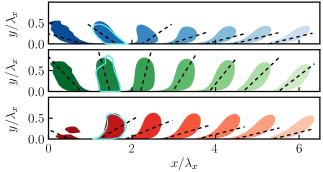
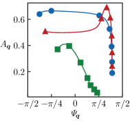
(a)  (b)

Figure 1: Evolution of the amplitude and inclination angles of an optimal transient growth mode in a channel flow. $\lambda_{x}=\lambda_{z}$. (a) Snapshots of the velocity components (top to bottom, $u$, $v$, $w$), spaced by $St\approx 0.52$, from left to right. The dashed lines show the inclination angle computed as in Jiménez (2015). The contours levels are $u=4,v=1,w=3$ in uniform arbitrary units. (b) Amplitude as a function of the inclination angle. The markers are, , $u$; , $v$; , $w$; and correspond to the snapshots in (a)

For more complex mean velocity profiles, Orr-like solutions can be computed numerically. We use the algorithm in Schmid & Henningson (2001) to find solutions that optimally amplify the total kinetic energy, including a $y$-dependent eddy viscosity to account for the nonlinear turbulent dissipation, and a velocity profile and kinematic viscosity corresponding to a turbulent channel at $\Rey_{\tau}=u_{\tau}h/\nu=2000$, as in del Álamo & Jiménez (2006) and Pujals et al. (2009). We use the approximation to the mean eddy viscosity $\nu_{T}$ of Cess (1958):

$$\nu_{T}=\frac{\nu}{2}\left\{1+\frac{K^{2}\Rey_{\tau}}{9}\left[2\eta-\eta^{2}\right]\left[3-4\eta+\eta^{2}\right]^{2}\left[1-\exp{\left(\frac{-\eta\Rey_{\tau}}{A}\right)}\right]^{2}\right\}^{1/2}+\frac{1}{2},$$ (7)

where $\eta=y/h$, and the parameters $A=25.4$ and $K=0.426$ are tuned to match the profile of Hoyas & Jiménez (2006). The mean velocity profile is obtained by integrating $\left(1-\eta\right){u_{\tau}}^{2}/{\nu_{T}}$. Using the same profiles, del Álamo & Jiménez (2006) found that the maximum energy amplification occurs for $\lambda_{x}\gg\lambda_{z}$, but Jiménez (2018) remarked that these wavenumbers are associated with the slow amplification of the streamwise-velocity streaks through (5), and to very long evolution times that may be limited by the nonlinear or viscous effects mentioned above. We are here interested in situations such as (6), where the energy amplification is associated with the transient bursting of $v$ over a few shear times. These were shown by Jiménez (2018) to be strongest at $\lambda_{x}\approx\lambda_{z}$.

Figure 1(a) shows as shaded contours several snapshots of the most amplified transient mode with $\lambda_{x}=\lambda_{z}\approx 0.7h$, plotted at intervals of $S(y_{g})\rmDelta t\approx 0.23$, where $S(y_{g})$ is the shear at the centre of gravity of the $v^{2}$ profile at maximum amplification. It was shown in Jiménez (2013) that the dimensions of the most amplified inviscid $v$-modes in the logarithmic layer are proportional to $\lambda_{0}=2\pi/(k_{x}^{2}+k_{z}^{2})^{1/2}$, and that their centre of gravity is at $y_{g}\approx 0.22\lambda_{0}$, or $y_{g}\approx 0.16\lambda_{x}$ for equilateral wavevectors. The same is true in figure 1(a), even if this case differs from Jiménez (2013) in using an eddy viscosity. The temporal evolution of the perturbations in Jiménez (2013) is controlled by $\lambda_{0}S(y_{g})t/\lambda_{x}$. In the range of wavelengths $250\nu/u_{\tau}\lesssim\lambda_{x}\lesssim 4h$, corresponding to $40\nu/u_{\tau}\lesssim y_{g}\lesssim 0.64h$, we can assume that $S(y_{g})\propto u_{\tau}/y_{g}\propto u_{\tau}/\lambda_{0}$, and that the scaling of the time is $\lambda_{0}S(y_{g})t/\lambda_{x}\propto u_{\tau}t/\lambda_{x}$. The result is that both the dimensions and the temporal evolution of the amplified structures scale with $\lambda_{x}$. The relation between the inclination angle $\Psi$ and the amplitude of $v$ was shown in Jiménez (2013) to be fairly independent of the wavenumbers, and even of the type of flow. These results are extended here to the three velocity components, and to the eddy-viscosity equations, and we indeed find that the optimal modes in the neighbourhood of $\lambda_{x}\approx\lambda_{z}$ scale well with $\lambda_{x}$ in the range of wavenumbers mentioned above. For example, the shape and inclination angles of the solution in figure 1(a) are remarkably similar to those in figure 19 of Jiménez (2018), where the wavelengths are much larger, $\lambda_{x}=3.9h,\lambda_{z}=5.55h$, and the solid contour lines superimposed on the second snapshot in figure 1(a), which show the moment of maximum amplitude of a mode with $\lambda_{x}=\lambda_{z}\approx 0.35h$, also agree very well with those at the longer wavelengths. The self-similar behaviour ceases to hold at heights corresponding to the buffer layer, where the shear is no longer inversely proportional to $y$.

The dashed lines in figure 1(a) are the vertically averaged inclination angles at each time, computed using the formula for single modes in Jiménez (2015); for a more general one see (18) below. They represent well the instantaneous structure of $v$, but they are biased towards the lower half of the structures for $u$ and $w$ because the averaging in (18) is weighted with the energy, which tends to be concentrated near the wall for these two components. This is also where the shear is highest, leading to flatter inclinations. Figure 1(b) shows the amplitude–inclination relation for the three velocity components in figure 1(a). The amplitude and inclination angles of the wavetrain are defined as in (Jiménez, 2015). Both definitions are extended in (17)–(18), later in this paper, to more general wavepackets. The trajectory for $v$ is reminiscent of (6), but the wall-parallel components tilt forwards much faster, as shown by the larger separation of their first few symbols, which are uniformly spaced in time. Inspection of figure 1(a) shows that this is also due to the weighting of the angle close to the wall, where the higher shear results in faster characteristic times. The upper part of the $u$ and $w$ structures does not tilt much faster than that of $v$, while the root of the latter tilts as fast as those of the other two components. The last half of the angle–amplitude evolution is also different for the three velocity components. The spanwise velocity has an amplitude peak at approximately the same time as $v$, which is not present for $u$. At the end of the evolution, $v$ decays at a rate dictated by the shear, while $u$ and $w$ only decay under the effect of the eddy viscosity. For inviscid perturbations in a uniform shear, the three velocity components have well-differentiated behaviours. During the burst, $v$ grows and decays in $t=O(S^{-1})$, as in (6), but $u$ and $w$ never decay (Jiménez, 2013). In all cases, continuity requires that the two wall-parallel have to be proportional to each other once $v$ has died. An important message of figure 1 is that optimum growth solutions should only be taken as indicative. The properties enumerated in the last few sentences are common to any initial condition, while optimum growth is meaningless in an inviscid flow. The behaviour of $v$, whose equation (4) is autonomous, is essentially independent of the initial conditions, which mostly define the origin of time, but $u$ and $w$ satisfy the forced equation (5), whose evolution depends on $v$ and on the initial conditions. The optimum transient growth criterion selects the initial condition with a highest local maximum, but the $v$ burst and the $v$-less final decay are robust properties of most initial conditions involving backwards-leaning perturbations. Note also that the energy growth in figure 1(b) is not particularly large, and that the same is true of all the cases mapped in figure 29 of Jiménez (2018).

3 Methods

The rest of the paper seeks to relate the behaviour of fully nonlinear channel flow simulations to the linearised dynamics sketched above.

3.1 The numerical datasets

Case	$\Rey_{\tau}$	$L_{x}/h$	$L_{z}/h$	$N_{x}$	$N_{y}$	$N_{z}$	$D_{y}$	$N_{f}$	$T_{\mkern-1.0muh}$		Reference
S1000	932	$2\pi$	$\pi$	$512$	$385$	$512$	CH	$1800$	20		Lozano-Durán & Jiménez (2014)
L1000	934	$8\pi$	$3\pi$	$2048$	$385$	$1536$	CH	$72$	8	.5	del Álamo et al. (2004)
S2000	2009	$2\pi$	$\pi$	$1024$	$633$	$1024$	FD	$590$	11		Lozano-Durán & Jiménez (2014)
F2000	2000	$8\pi$	$3\pi$	$512$	$512$	$512$	FD	$1146$	14		Vela-Martín et al. (2018)
L2000	2003	$8\pi$	$3\pi$	$4096$	$633$	$3072$	FD	$30$	10	.3	Hoyas & Jiménez (2006)
S4000	4164	$2\pi$	$\pi$	$2048$	$1081$	$2048$	FD	$40$	10		Lozano-Durán & Jiménez (2014)

Table 1: Parameters of the simulations. $L_{x,z}$ are the streamwise and spanwise periods of the numerical box. $N_{x,y,z}$ are the number of collocation grid points in $y$, or Fourier modes in $x,z$, except for F2000, which was computed at full resolution but stored at the reduced one given in the table. $D_{y}$ represents the discretisation used for the wall-normal direction: ‘CB’ refers to Chebyshev polynomials and ‘FD’ to compact finite differences. $N_{f}$ is the number of fields used to compute statistics. $T_{h}$ is the time spanned by the approximately equidistant $N_{f}$ snapshots in eddy turnover times. The snapshots of S1000 and F2000 are close enough in time to compute temporal derivatives.

We use direct simulations of canonical incompressible turbulent channel flows whose half-height is $h$. Normalisation with $\nu$ and $u_{\tau}$ is represented by a ‘$+$’ superscript, and our primary Reynolds number is $Re_{\tau}=h^{+}$. The simulations use periodic boundary conditions in the wall-parallel directions, with periods $L_{x}$ and $L_{z}$, and are summarised in table 1. The Reynolds numbers range from $\Rey_{\tau}\approx 900\text{ to }4000$, and the simulations include both medium-sized $(L_{x}=2\pi h,L_{z}=\pi h)$ and large $(L_{x}=8\pi h,L_{z}=3\pi h)$ computational boxes. The equations of motion are written as evolution equations for the $(x,z)$ averages of the streamwise and spanwise velocities, and for $\phi$ and $\omega_{y}$, as in (4)–(5) without linearisation (Kim et al., 1987). The spatial discretisation is Fourier spectral in the two periodic directions, dealiased using the pseudo-spectral 3/2 rule, but the discretisation along $y$ varies among simulations, as indicated in table 1. Some cases use Chebyshev polynomials collocated at the Gauss–Lobatto–Chebyshev nodes. Others use spectral-like compact finite differences (Lele, 1992; Flores & Jiménez, 2006), up to 12th-order consistent, in grids whose spacing is adjusted to keep the resolution approximately constant in terms of the local isotropic Kolmogorov scale $\eta=(\nu^{3}/\varepsilon)^{1/4}$. Full details can be found in the original publications. F2000 has the peculiarity of being run as a direct numerical simulation, but stored at a coarser ‘large-eddy simulation’ resolution (Vela-Martín et al., 2018). The data stored are snapshots of the three velocity components, which in most cases are approximately statistically independent and can only be used to compile instantaneous statistics. However, the snapshots in S1000 and F2000 are stored closely enough in time to provide temporal derivatives and histories without recomputing the flow evolution.

3.2 Filtering

As discussed in §2, the relation between the instantaneous tilting angle of the wall-normal velocity perturbations and their amplitude can be used as a diagnostic property for Orr bursts. Jiménez (2015) defined the inclination angle of the wavefronts of a pure Fourier mode in terms of the wall-normal derivative of its complex phase, but this definition, as well as that of the amplitude, needs to be generalised for spatially localised objects. Consider the low-pass-filtered field

$$\widetilde{\boldsymbol{q}}(x,y,z,t;\Lambda)=\int_{\mathcal{B}}\Gamma(x^{\prime}-x,z^{\prime}-z,\Lambda)\boldsymbol{q}(x^{\prime},y,z^{\prime},t){{\,\rm{d}}}x^{\prime}{{\,\rm{d}}}z^{\prime},$$ (8)

where $\mathcal{B}$ stands for the full computational box, $\varLambda$ serves as the filter width and

$$\Gamma(x,z;\Lambda_{0L},\Lambda_{0z})=\gamma(x,\Lambda_{0L})\,\gamma(z,\Lambda_{0z}),$$ (9)

with

$$\gamma(\xi,\Lambda_{0})=\frac{1}{\Lambda_{0}\sqrt{2\pi}}\exp\left[-\tfrac{1}{2}(\xi/\Lambda_{0})^{2}\right];$$ (10)

and the band-pass-filtered one

$$\overline{\boldsymbol{q}}(x,y,z,t;\Lambda)=\int_{\mathcal{B}}G(x^{\prime}-x,z^{\prime}-z,\Lambda)\boldsymbol{q}(x^{\prime},y,z^{\prime}){{\,\rm{d}}}x^{\prime}{{\,\rm{d}}}z^{\prime},$$ (11)

with

$$G(x,z;\Lambda,\Lambda_{0x},\Lambda_{0z})=\Gamma(x,z;\Lambda_{0x},\Lambda_{0z})\exp(2\pi{\rm i}x/\Lambda).$$ (12)

The spectral transfer functions of the two kernels are

$$|\widehat{\Gamma}|^{2} = \exp\left[-(k_{z}\Lambda_{0z})^{2}-(k_{x}\Lambda_{0L})^{2}\right],$$ (13)

$$|\widehat{G}|^{2} = \exp\left(-(k_{z}\Lambda_{0z})^{2}-[(k_{x}-2\pi/\Lambda)\Lambda_{0x}]^{2}\right),$$ (14)

where the carat stands for the $(x,z)$ Fourier transform. Both filters have spectral width $\rmDelta k=O(\Lambda_{0}^{-1})$, but the band-pass filter $G$ is centred at the wavenumber $k_{x}=2\pi/\Lambda$ (and $k_{z}=0$), while the low-pass filter $\Gamma$ is centred at $k_{x}=k_{z}=0$. Thus, if $\Lambda$ and the $\Lambda_{0}$’s are chosen to be of the same order, $\Gamma$ smooths the flow by damping everything shorter and narrower than $O(\Lambda_{0})$, while $G$ selects only structures which may be wide, but whose length is of the order of $\Lambda$. The latter is useful to isolate localised bursts, while the former also retains the larger structures of the flow around them.

The low-pass filter $\Gamma$ presents few conceptual problems, and its results are described in §5, but the band-pass filter (11) generates a complex field which is not easily interpreted as a flow, and requires some discussion. Its kernel $G$ is a monochromatic complex wave in the streamwise direction whose amplitude is modulated by the Gaussian (10) in the streamwise and spanwise directions. It is essentially a complex-valued continuous Morlet or Gabor wavelet (Farge, 1992), whose real and imaginary parts are represented in figure 2(a) as functions of $x$. The number of oscillations contained within the Gaussian envelope is approximately $2\Lambda_{0x}/\Lambda$. To keep the filters self-similar we choose $\Lambda_{0x}=\Lambda/2$ and $\Lambda_{0z}=\Lambda/6$, implying an aspect ratio $\Lambda_{0x}:\Lambda_{0z}\approx$ $3:1$, which captures the strongest wall-normal velocity perturbations (see figure 3b). Changing this aspect ratio to $2:1$ or 4:1 did not qualitatively change the results.

The main advantage of filtering a real-valued function with a complex wavelet is that the real and imaginary parts of the resulting field preserve phase (positional) information, while its absolute value hides the oscillations of the wavelet (Sreenivasan, 1985; Farge, 1992). A visualisation for synthetic data is presented in figure 2(b).

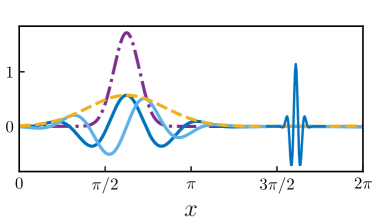
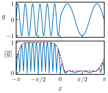
(a)   (b)(c)

Figure 2: (a) The wider filter on the left is the band-pass kernel $G(x,0)$ for $\Lambda={4\pi}/{9}$. The solid darker line is $\operatorname{Re}(G)$, and the lighter one is $\operatorname{Im}(G)$. The two envelopes are: , $\gamma(x,\Lambda_{0L})$; , $\gamma(x,\Lambda_{0z})$. The narrower filter on the right corresponds to $\Lambda={\pi}/{18}$, although the amplitude has been divided by four for the purpose of plotting. (b) Sample signal, $g=\sin(12x)\text{ if }x<0$, and $\sin(3x)$ otherwise. (c) Its amplitude after band-pass filtering with $\Lambda=\pi/6$. The solid line in (c) is the amplitude $|\operatorname{Re}(G)|$, and the dashed one corresponds to $|G|$.

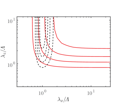
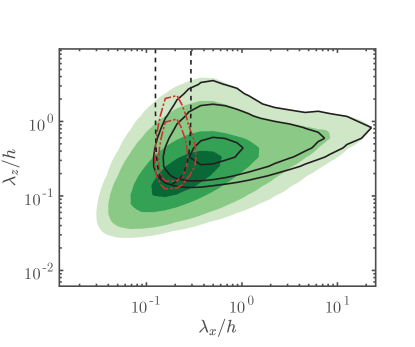
(a)(b)

Figure 3: (a) Transfer functions of the: , band-pass filter $G$;   , low-pass filters $\Gamma$. The contours are $(0.2:0.2:0.8)$. (b) Sample filtered premultiplied spectra of $v$ in L2000, at $y/h=0.15$ and $\Lambda/h=0.175$. The dashed contour is $|\widehat{G}|^{2}=0.2$. The shaded contours are the full $k_{x}k_{z}E_{vv}$;   , low-pass filtered; , band-pass filtered. The spectral contours are $k_{x}k_{z}E_{vv}/u_{\tau}^{2}=(0.014,0.029,0.071,0.114)$.

In fact, the band-passed field, $\overline{a}$, of a generic velocity component can be interpreted as the coefficient of a local Fourier expansion that optimally approximates the flow within the Gaussian envelope (9). It minimises the weighted $L_{2}$ error

$$J[\overline{a}](x)=\int_{\mathcal{B}}\Gamma\left(x^{\prime}-x,z^{\prime}-z\right)\left|a(x^{\prime},y,z^{\prime})-\overline{a}^{\dagger}(x,y,z)\exp\left[2\pi{\rm i}(x^{\prime}-x)/\Lambda\right]\right|^{2}{\,\rm{d}}x^{\prime}{\,\rm{d}}z^{\prime},$$ (15)

where the dagger denotes complex conjugation and $a$ is either $u$, $v$ or $w$. Note that $a^{\dagger}$ in this integral is evaluated at the centre of the filtering kernel, $x$, rather than at the integration variable, $x^{\prime}$, and that the Fourier wavetrain, $\exp\left[2\pi{\rm i}(x^{\prime}-x)/\Lambda\right]$, is centred in each case at the filter position. This implies that $a^{\dagger}$ can be interpreted as a field of coefficients of ‘local’ Fourier wavetrains, whose absolute value is $\left|a(x,y,z)\right|$, and whose argument is $-\arctan(\operatorname{Im}(a)/\operatorname{Re}(a))$. Thus, although $\overline{\boldsymbol{q}}$ cannot be used as a filtered velocity field, its absolute value is the local wavetrain amplitude (Sreenivasan, 1985), and the wall-normal derivative of its argument is a local inclination angle, as in Jiménez (2015).

It is convenient to choose the short-wave limits of the low-pass and band-pass filters to be of the same order, so that they isolate related structures. The (1/e) limit of (14), i.e. the argument that makes the filter gain equal to $(1/e)$, is $k_{x}=2\pi/\Lambda+1/\Lambda_{0x}$, while that of (13) is $k_{x}=1/\Lambda_{0L}$. Equating them results in $\Lambda_{0L}=\Lambda/(2\pi+\Lambda/\Lambda_{0x})$. For our previous choice of $\Lambda_{0x}=\Lambda/2$, this implies $\Lambda_{0L}=\Lambda/8$. The transfer function of the two filters is represented in figure 3(a). The cospectrum of any two filtered variables can be computed from the unfiltered cospectrum as $E_{\overline{a}\,\overline{c}}=E_{ac}|\widehat{G}|^{2}$, with an equivalent formula for $E_{\widetilde{a}\widetilde{c}}$. An example of the effect of the band- and low-pass filters on the spectrum of a representative plane of $v$ is shown in figure 3(b).

Note that the computation of the filtered fields can be done economically because the streamwise and spanwise directions are periodic, and fast Fourier transforms can be used to compute the convolutions (Canuto et al., 1988).

3.3 The band-pass-filtered pseudo-spectrum

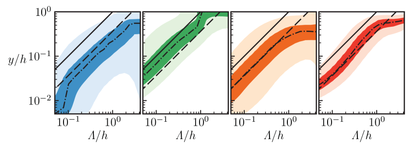
(a)(b)(c)(d)

Figure 4: Pseudo-spectra of the band-pass filtered velocity components and of their tangential Reynolds stress, as a function of the filter wavelength and of the distance from the wall. $Re_{\tau}=5200$ (Lee & Moser, 2015). The contours are 90% and 50% of the maximum as a function of $y$, for each filter wavelength. The solid and dashed lines bracket the most energetic part of $\mathcal{E}_{vv}$ in (b). The upper (solid) limit is $y=\Lambda$. The lower (dashed) one is $y=4\Lambda/11$. The chain-dotted line is the wall-normal location of the maximum for each filter width. (a) $\mathcal{E}_{uu}$. (b) $\mathcal{E}_{vv}$. (c) $\mathcal{E}_{ww}$. (d) $-\mathcal{E}_{uv}$.

The perturbation energy of the filtered flow fields can be directly computed from their spectrum:

$$\mathcal{E}_{ac}(y;\Lambda)=\sum_{\forall k_{x},k_{z}}E_{\overline{a}\,\overline{c}}(k_{x},y,k_{z};\Lambda)=\sum_{\forall k_{x},k_{z}}|\widehat{G}|^{2}(k_{x},k_{z};\Lambda)E_{ac}(k_{x},y,k_{z}),$$ (16)

which is represented in figure 4 for the three velocity components and for the tangential Reynolds stress, as a function of $y$ and of the filter wavelength $\Lambda$. Because the filter wavelength represents the size of the scales retained by the filter, we can think of $\mathcal{E}_{ac}(y;\Lambda)$ as a ‘pseudo-spectrum’ with pseudo-wavelength $\Lambda$. Figure 4 shows that the wall-normal location of the maximum energy is proportional to the filter width for a range of heights corresponding to an extended logarithmic layer, $y\in(100\nu/u_{\tau},0.4\,h)$. This is also approximately the region where a self-similar hierarchy of wall-attached velocity structures with sizes proportional to their distance from the wall is found to exist (Townsend, 1976), and we will refer to it as our definition of the logarithmic layer from now on. Note that, although the filter is self-similar in the streamwise and spanwise directions, it contains no information about the sizes in $y$, and thus the uncovered self-similarity in $y$ is not a property of the filter, but of the spectra of the velocity components. Owing to the removal of the large scales by the filter, the wall-parallel velocities also show long self-similar ranges, albeit centred at larger scales. This was shown also to be the case in Abe et al. (2018), where a minimal streamwise unit was used to remove the large scales of $w$, uncovering a self-similar behaviour for this component.

Figure 4 allows us to determine which distances from the wall should be used to characterise eddies of different scales. The band-pass filter (12) produces a flow field that is locally averaged within each wall-parallel plane, but eddies and bursts also have a vertical dimension, which figure 4 shows to be proportional to their horizontal ones (Lozano-Durán et al., 2012). It was shown by Jiménez (2013) that bursts may be characterised by a vertically averaged amplitude,

$$A^{2}_{\overline{a}}=\frac{1}{y_{1}-y_{0}}{\int_{y_{0}}^{y_{1}}\left|\overline{a}\right|^{2}{{\,\rm{d}}}y},$$ (17)

and by a mean inclination angle,

$$\Psi_{\overline{a}}=\arctan\dfrac{\Lambda\int_{y_{0}}^{y_{1}}\operatorname{Im}(\overline{a}^{\dagger}\partial_{y}\overline{a}){{\,\rm{d}}}y}{2\pi\int_{y_{0}}^{y_{1}}\left|\overline{a}\right|^{2}{{\,\rm{d}}}y},$$ (18)

where $a$ stands for either $u$, $v$ or $w$, and the integrals extend over the intense part of the eddy. The average in (18) is weighted with the square of the amplitude because strong perturbations typically coexist in the filtering window with weaker ones, whose inclination angle is not necessarily small, nor relevant.

The limits $y_{0}$ and $y_{1}$ are chosen to bracket the intense band of $\mathcal{E}_{vv}$ in figure 4(b), and the same limits are used for all variables. The upper limit is very close to the Corrsin spectral scale, $y_{1}=\Lambda$, above which the shear is too weak to interact with eddies of size $\Lambda$ (Jiménez, 2018). The lower limit, $y_{0}=4\Lambda/11$, also scales with $\Lambda$, and represents the point below which impermeability damps $v$. Because these limits are adjusted for the wall-normal velocity, while the $u$ or $w$ structures are larger than those of $v$, figure 4(a, c) shows that they are too far from the wall to capture more than a fraction of the energy of the wall-parallel components. Approximately energy of the band-passed spanwise component is captured within the band, closer to the lower limit, potentially associated with the short scales of $w$. Longer features of $w$ fall outside the band, and probably come from larger structures farther away from the wall (del Álamo et al., 2004). On the other hand, the tangential Reynolds stress in figure 4(d) is captured well, supporting the classical classification into ‘active’ and ‘inactive’ eddies of Townsend (1976), as a substantial amount of longer $u$ and $w$ perturbations carry little tangential Reynolds stress.

From now on, we will use the quantities in (17)–(18) to represent the local amplitude and inclination angle of our flow fields. Their main practical advantage is that they reduce the dimensionality of our dataset, because each filter has an associated three-dimensional data space (the two wall-parallel positions and time), instead of the full four-dimensional one. In addition, they act as a filter in $y$, excluding structures outside the band $(y_{0},\,y_{1})$, or with very different vertical dimensions from the band thickness. They are centred at $[x,(y_{0}+y_{1})/2,z]$, and the vertical average is only meaningful whenever a velocity perturbation of size comparable to $\Lambda$ happens to be within the vertical integration window. Otherwise, the average reverts to the unconditional mean. For example, when several wavetrains with different inclinations are stacked along the wall-normal direction, the integral of their phase derivatives produces an average inclination angle which is similar to the global ensemble-averaged inclination.

3.4 Filter parameters

Table 2 gathers the information for the filters used in the paper. We use six wavelengths,

$$\Lambda_{i}/h=\frac{8\pi}{9}2^{-i},\quad i=1,\ldots 6,$$ (19)

with the corresponding filtered fields denoted by $\overline{\boldsymbol{q}}_{i}=\overline{\boldsymbol{q}}(x,y,z,t;\Lambda_{i})$ for the band-pass filters discussed in §4, and $\widetilde{\boldsymbol{q}}_{i}=\widetilde{\boldsymbol{q}}(x,y,z,t;\Lambda_{i})$ for the low-pass ones in §5. They cover the energy spectrum with logarithmically equispaced bands of wavelengths, and span the range that can be expected to be relevant for the logarithmic layer. The long-wavelength limit of the widest filter is kept constant in outer units across Reynolds numbers, $\Lambda_{1}/h={4\pi}/{9}$. It follows from figure 4 that this filter corresponds to $y/h\in(0.5,\,1.4)$, which is well above the expected self-similar region, but it is retained here to compare it to the experiments in Jiménez (2015), who analysed the first streamwise mode of a minimal channel with $L_{x}={\pi}/{2}$. It allows us to test whether the minimal domain used in that work affected the results. The short-wavelength limit, $\Lambda^{+}\approx 180$, scales in wall units, resulting in an increasing number of filter bands as the Reynolds number increases. In the highest Reynolds number case S4000, this filter corresponds to $\Lambda_{6}$. Since both our Reynolds numbers and our filter widths are approximately spaced by powers of two, there are matching filters for all the simulations, both in outer and in inner units, allowing us to compare scaling criteria.

Name	$\Lambda/h$	$y_{0}/h$	$y_{1}/h$	S1000	L1000	S2000	F2000	L2000	S4000
$\Lambda_{1}$	$1.4$	1.0	0.51	$\circ$	$\circ$	$\circ$	$\circ$	$\circ$	$\circ$
$\Lambda_{2}$	$0.7$	0.7	0.25	$\circ$	$\circ$	$\circ$	$\circ$		$\circ$
$\Lambda_{3}$	$0.35$	0.35	0.13	$\circ$	$\circ$	$\circ$	$\circ$		$\circ$
$\Lambda_{4}$	$0.175$	0.175	0.063	$\circ$	$\circ$	$\circ$	$\circ$		$\circ$
$\Lambda_{5}$	$0.087$	0.087	0.032			$\circ$			$\circ$
$\Lambda_{6}$	$0.044$	0.044	0.016						$\circ$

Table 2: Properties of the filters used. $\Lambda$ is the filter width defined in (12), and $y_{0}$, $y_{1}$ are the integration limits in (17)–(18). A circle below a simulation indicates that that filter was computed for it.

To estimate how much energy is retained by our band-pass filtering and vertical integration operations, we compute the ratio between the energy of the filtered and unfiltered wall-normal velocity field within a given band of wall distances, as a function of the filter wavelength. It ranges from $10\%$ to $20\%$, with the higher limit corresponding to the narrower filters. These values are similar to that for the single most energetic mode in Jiménez (2015). In our case, we can study multiple sizes covering a broad range of scales, but the quantification of the total filtered energy is not straightforward because the spectral and wall-normal bands of the filters overlap. One way of getting the equivalent to a Parserval’s theorem for localised basis functions would be to project the velocity onto an orthonormal wavelet basis instead of using continuous wavelets (Meneveau, 1991), but at the cost of limiting the spatial locations at which we could have information of a given scale, making it unsuitable for smoothly tracking the temporal evolution of the structures. Another approach is to rescale the kernels so that they recover the total energy when integrated over scale space (Leung et al., 2012), but this distorts the amplitudes, and only works for a particular spectrum. We have chosen to make our transfer functions unity at their nominal wavelength. The energy contained in the overlap of neighbouring filters is then about 2%–5% (non-neighbouring bands are irrelevant because they do not overlap vertically). Accounting for overlaps, our filters approximately retain 20% of the total energy of the wall-normal velocity in $60~{}\nu/u_{\tau}<y<h$ at $Re_{\tau}=2000$, with minor differences among Reynolds numbers. This energy ratio concerns the band-pass filter that is designed to isolate the bursts. The less isolating low-pass filter retains 50%($\Lambda_{1}$)–70%($\Lambda_{4}$) of the turbulent kinetic energy, and we will see through the paper that most of the conclusions obtained for the band-passed structures carry over to the low-passed ones.

4 Band-pass-filtered amplitude and inclination fields

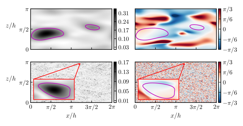
Figure 5: Snapshots of the amplitude, $A^{+}_{{\overline{v}}}$(left), and inclination angle, $\Psi_{{\overline{v}}}$(right), of the band-pass-filtered wall-normal velocity of S4000. Top corresponds to $\overline{v}_{1}$ and bottom to $\overline{v}_{6}$. While the top snapshot has been carefully picked to contain a burst at this scale, the bottom one is randomly chosen, because all snapshots contain at least one burst. The inset amplifies a region of $\overline{v}_{6}$ with a burst. The amplification factor, 32, corresponds to the wavelength ratio between both filters. The contours are $A^{+}_{\overline{v}}=0.5\max{\{A^{+}_{\overline{v}}\}}$.

Figure 5 shows snapshots of the amplitude and inclination angle of the band-pass-filtered wall-normal velocity, as defined in (17)–(18). Figure 5(a, b) uses the widest of our six filters, $\overline{v}_{1}\,(\Lambda=1.4h)$, while figure 5(c, d) uses the narrowest one, $\overline{v}_{6}\,(\Lambda=0.044h)$, which is 32 times narrower. To facilitate comparison, the insets in figures 5(c, d) are magnified by the ratio of the two filter widths, resulting in structures of similar size to those in figures 5(a, b). This supports our remark in §3.2 that the band-pass filter isolates structures of size proportional to $\Lambda$. The amplitude fields in figures 5(a, c) are smooth, with distinct intense regions which are candidates for Orr events at the moment of peak amplitude. They are highlighted as line contours in both the amplitude and inclination fields, and it is visually clear from figures 5(b, d) that the regions of high intensity are associated with vertical inclinations.

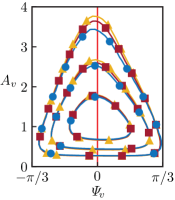
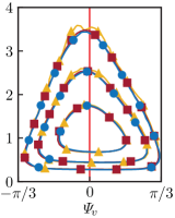
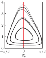
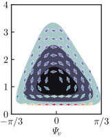
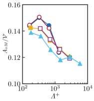
(a) ${A_{\overline{v}}}/{A_{\overline{v}M}}$ (b) (c)
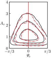
(d) ${A_{\overline{v}}}/{A_{\overline{v}M}}$ (e) (f)

Figure 6: (a–e) Joint p.d.f.s of the amplitude, $A_{{\overline{v}}}$, and inclination angle, $\Psi_{{\overline{v}}}$, of the filtered wall-normal velocity. The amplitudes are normalised with their mode, given in (f). Contours contain $50,90,99\%$ of the probability mass. (a) Joint p.d.f. of $\overline{v}_{3}$ for S1000, S2000 and S4000. (b) Joint p.d.f. of $\overline{v}_{3},\overline{v}_{4},\overline{v}_{5}$ for S1000, S2000 and S4000, respectively. (c) Averaged joint p.d.f. for the filters that fall in the logarithmic region, $\overline{v}_{2}$ to $\overline{v}_{6}$, for the available cases, as in table 2. The solid lines are the averaged p.d.f.. The dashed lines along each contour bracket the minimal area that contains all of the individual joint p.d.f.s. (d) The solid lines are the average of all the joint p.d.f.s of $\overline{v}_{1}$. The chain-dotted red line is as in figure 3 in Jiménez (2015). (e) Joint p.d.f. of $\overline{v}_{3}$ for F2000. The arrows are the conditional mean velocities (CMV), normalised to unit length. The colours are the standard deviation of the CMVs normalised with their mean, ranging from 0.4 (dark blue) to 6.5 (red). (f) Modal values used to normalise the amplitudes. Symbols: , S1000; , L1000; , S2000; , F2000; , L2000; , S4000.

The joint probability density function (p.d.f.) of $A_{\overline{v}}$ and $\Psi_{\overline{v}}$ is presented in figure 6(a–e), with the amplitude normalised by the modal value, $A_{{\overline{v}}M}$, at which its p.d.f. is maximum. As in Jiménez & Hoyas (2008), the p.d.f.s collapse better in this normalisation than with the mean. While figure 5 emphasises the self-similarity of the filtering operation, figure 6(a–c) tests the self-similarity of the filtered flow, which should hold both in inner and in outer units throughout the logarithmic region. Figures 6(a) and 6(b) each includes p.d.f.s at three Reynolds numbers, but those in figure 6(a) have the same filter width in outer units $(\Lambda/h=0.35)$, and those in figure 6(b) have the same width in inner units $(\Lambda^{+}\approx 350)$. In both cases, the p.d.f.s agree well. Figure 6(c) collects the p.d.f.s for all the Reynolds numbers and all the filters whose vertical domain is contained within the logarithmic region (see table 2). The solid contours are the average of all the p.d.f.s, and the dashed ones bracket the narrowest band that contains the corresponding contours of all the cases. It is clear from these results that the similarity of the p.d.f.s is satisfied extremely well.

Figure 6(d) displays the p.d.f. of the widest filter $\overline{v}_{1}$, averaged over all the flows in table 2. This filter is too wide to collapse with the ones in the logarithmic layer, but all the p.d.f.s used in figure 6(d) also agree well among themselves (not shown). The averaged p.d.f. is compared in the figure with the results in Jiménez (2015), who analysed a single Fourier mode of wavelength comparable to $\Lambda_{1}$. The good agreement validates the approximate equivalence between the new methodology and the monochromatic analysis in Jiménez (2015).

The collapse of the p.d.f.s in figure 6 also supports that the behaviour of the $v$-bursts is relatively independent of the numerical box. Figure 6(a–e) contains p.d.f.s from a variety of numerical boxes, which agree well among themselves, and the p.d.f. from Jiménez (2015) in figure 6(d) uses a very small box, $L_{x}/h=\pi/2,L_{z}/h=\pi/4$, which only represents well the structures below $y/h\approx 0.25$, but which is too small for the larger ones farther from the wall.

The p.d.f.s in figure 6 have two distinct regions. Their core, which includes most of the probability mass, contains vertically oriented structures with amplitudes of the order of the modal value $A_{{\overline{v}}M}$. That the typical inclination of $v$ in channels is vertical had previously been shown using proper orthogonal decomposition by Moin & Moser (1989), and using autocorrelation functions by Sillero et al. (2014).

The upper part of the outermost isocontour of the p.d.f.s contains large amplitudes and inclinations, and is approximately triangular. The extreme values and low probabilities in this region suggest that these points represent individual structures, while the triangular shape implies a definite statistical relation between the inclination angle and the intensity, as graphically suggested by figure 5. Weak regions are inclined either forwards or backwards, and strong ones are approximately vertical or slightly tilted backwards, as in the transient linearised bursts discussed in §2.1.

Moreover, the upper part of the p.d.f. is traversed from left to right, as expected of shear-dominated structures. This was already shown to be the case for monochromatic wavetrains in Jiménez (2015), but is confirmed here for localised structures in large boxes. In the time-resolved cases, S1000 and F2000, we can define conditional mean velocities (CMVs) in the $(\Psi_{\overline{v}},A_{\overline{v}})$ parameter space as

$$\bigg{\langle}\left[\frac{{{\rm{D}}}\Psi_{\overline{v}}}{{{\rm{D}}}t},\frac{{{\rm{D}}}A_{\overline{v}}}{{{\rm{D}}}t}\right]\bigg{\rangle}_{(\Psi_{\overline{v}},A_{\overline{v}})},$$ (20)

where $\langle\,\rangle_{(\Psi_{\overline{v}},A_{\overline{v}})}$ denotes conditional averaging at $(\Psi_{\overline{v}},A_{\overline{v}})$, and ${\rm{D}}/{\rm{D}}t=\partial_{t}+C_{\!\Lambda}\partial_{x}$, is a semi-Lagrangian approximation to the total derivative that incorporates an advection velocity, $C_{\!\Lambda}$, estimated by linear regression of the time-dependent $x$ location of the maximum of the $x$–$t$ two-point two-time autocorrelation of $A_{\overline{v}}$, using at each instant a centred seven-point time stencil. In this approximation, the advection velocity is assumed to be unique for the whole $(x,z)$ plane, independently of the number of bursts present at each moment, and depending only on the filter width. This is justified because the structures of the logarithmic layer were shown not to be dispersive by Lozano-Durán & Jiménez (2014) and by Jiménez (2018), and because the uniform scale of the band-pass-filtered variables would probably guarantee a uniform advection velocity even in they were. The rest of the temporal derivatives in (20) use five-point centred finite differences. Note that, although the advection velocity of individual structures is known to be approximately equal to the mean flow velocity, and is therefore a function of $y$, the velocity used here for the vertically integrated bursts is independent of the wall distance.

The result is presented in figure 6(e) for F2000, where the CMVs are plotted in the $(\Psi_{\overline{v}},A_{\overline{v}})$ plane as arrows pointing towards the next most probable state. The arrows are coloured by the conditional standard deviation of the CMV, which is high in the core and lower edge of the p.d.f., and low in its upper edge, as in Jiménez (2015). This suggests again that the mean velocities in the upper part of the p.d.f. are representative of individual coherent events, although it is unclear at this point whether the full periphery can be considered to represent a single burst, or whether it is formed by tangents of different burst trajectories at different locations.

While the coherent part of the p.d.f. is traversed from left to right, its lower part is traversed from right to left, closing the cycle. This is inconsistent with linear models, but the standard deviation of the CMVs in this region is large, suggesting that it is populated by structures that cannot be characterised solely by their position in the $(\Psi_{\overline{v}},A_{\overline{v}})$ plane, and whose evolution cannot be modelled by quasi-linear dynamics.

Finally, figure 6(f) shows the modal values used to normalise $A_{\overline{v}}$ in the rest of figure 6. Different box sizes yield the same modal value, which is fairly constant when compared with the wall-normal velocity fluctuation averaged within the same bands:

$$(\mathcal{V}^{\prime})^{2}=\frac{1}{y_{1}-y_{0}}\int_{y_{0}}^{y_{1}}(v^{\prime})^{2}{\,\rm{d}}y.$$ (21)

This constancy is a consequence of the self-similar definition of the filter, whose transfer function has constant logarithmic width in $\lambda_{x}$, independently of $y$ and $\Lambda$. Since figure 4 shows that the wavelengths of the spectrum of the wall-normal velocity also scale self-similarly with $y$, the energy selected by a truly self-similar filter should be approximately constant, but, because our band-pass filters are defined as low-pass in $\lambda_{z}$ (see §3.2), the transfer function of the narrower filters spans a wider range of $\lambda_{z}$. The extra energy in these wavelengths explains the slightly larger modal values of the narrow filters in figure 6(f).

4.1 Wall-parallel velocities

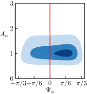
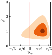
(a) ${A_{\overline{u}}}/{A_{\overline{u}M}}$             (b) ${A_{\overline{w}}}/{A_{\overline{w}M}}$

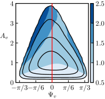
(c) ${A_{\overline{v}}}/{A_{\overline{v}M}}$       (d) ${A_{\overline{v}}}/{A_{\overline{v}M}}$

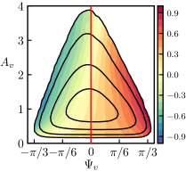
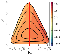
(e)       ${A_{\overline{v}}}/{A_{\overline{v}M}}$ (f) ${A_{\overline{v}}}/{A_{\overline{v}M}}$

Figure 7: Joint p.d.f.s of $A$ and $\Psi$ involving $\overline{u}_{3}$ and $\overline{w}_{3}$ for S1000. All amplitudes are normalised with their modal values. (a) $\Psi_{\overline{u}}$ and $A_{\overline{u}}/A_{{\overline{u}}M}$, contour levels are $90\%$, $50\%$ and $10\%$ of the probability mass. (b) $\Psi_{w}$ and $A_{\overline{w}}/A_{{\overline{w}}M}$, contours as in (a). (c–f) Black contours are the joint p.d.f. of $A_{{\overline{v}}}/A_{{\overline{v}}M}$ and $\Psi_{{\overline{v}}}$, contours containing $99.9\%$, $99\%$, $90\%$ and $50\%$ of the probability mass. Shaded contours are the mean of several quantities conditioned to the value of $A_{{\overline{v}}}$ and $\Psi_{{\overline{v}}}$. (c) Conditional average of $A_{\overline{u}}/A_{{\overline{u}}M}$. (d) $A_{\overline{w}}/A_{{\overline{w}}M}$. (e) $\Psi_{\overline{u}}$. (f) $\Psi_{\overline{w}}$.

We next compute the amplitude and inclination angles of the band-pass-filtered wall-parallel velocities. Figure 7(a, b) shows the joint p.d.f.s of $(\Psi,\,A)$ for $\overline{u}$ and $\overline{w}$, respectively. Their structures are preferentially tilted towards the direction of the shear, in contrast to the wall-normal velocity structures, which are almost equally distributed between forward and backward inclinations. This is more pronounced for the spanwise velocity, which is rarely tilted backwards (10% probability), and subtler for the streamwise component, which is tilted backwards 40% of the time. As with the wall-normal velocity, there is a statistical correlation between the amplitude and inclination of the spanwise velocity, but the same is not true for the streamwise velocity, for which the two quantities are essentially unrelated. Scrambling $A_{\overline{u}}$ with respect to $\Psi_{\overline{u}}$ leaves their joint p.d.f. unchanged (not shown). The behaviour of the inclination angles and amplitudes of $\overline{u}$ and $\overline{w}$ in the upper part of their joint p.d.f.s is qualitatively similar to the linearised trajectories in figure 1(b), although the inclination angles differ quantitatively. For example, the spanwise velocity shares with the transient-growth model an amplitude ‘peak’ towards positive inclinations, but the tilting angle of the linearised peak is always larger than that of the direct numerical simulation by 0.1–0.2 radians. Using unconditional two-point correlations of the wall-normal and spanwise velocity components, Jiménez (2018) argued that the cross-stream velocities contributing to the correlation are part of a quasi-streamwise ‘roller’. Some of the features of those autocorrelation functions are shared by the intense core of the joint p.d.f.s in figures 6 and 7. For example, the autocorrelation of the wall-normal velocity in the logarithmic layer is approximately vertical ($\Psi_{\overline{v}}\approx 0$), and the spanwise velocity is tilted forward by $\Psi_{\overline{w}}\approx\pi/6$, in agreement with the amplitude peaks of the joint p.d.f.s of $\overline{v}$ and $\overline{w}$. Because the correlation function is dominated by strong events, these similarities are not surprising, but they confirm that the band-pass filter retains some of the structure of the intense events of the velocity.

To explore the relation between the different variables during the bursting cycle, we compute averages conditioned to ($\Psi_{\overline{v}},A_{\overline{v}}$). The conditional mean amplitudes of $\overline{u}$ and $\overline{w}$ are presented in figures 7(c, d), and their conditional inclinations are shown in figure 7(e, f). If we assume that the CMVs in figure 6(e) reflect the temporal evolution of individual strong bursts, we can describe the burst by the evolution of the conditional mean values of the different quantities as we move from left to right along the upper edge of the p.d.f. of ($\Psi_{\overline{v}},A_{\overline{v}}$). The burst starts from intense $\overline{u}$, with weaker $\overline{v}$ and $\overline{w}$. At this stage $\overline{u}$ and $\overline{v}$ are tilted upstream, but $\overline{w}$ is too weak for its inclination to be defined. The ambient shear then tilts everything forward, and $\overline{v}$ and $\overline{w}$ are amplified while the amplitude of $\overline{u}$ decreases. Beyond the point where $\overline{v}$ is vertical, the amplitude of the wall-normal velocity decreases again, but $\overline{w}$ reaches its maximum value. The interpretation of these observations will be deferred to §4.2, after we have examined the conditional temporal behaviour of individual bursts.

4.2 Conditional mean evolutions

Number of bursts	Dataset	$\Lambda_{1}$	$\Lambda_{2}$	$\Lambda_{3}$	$\Lambda_{4}$
In total	S1000	$70$	$228$	$1301$	$9777$
In total	F2000	$863$	$5098$	$34802$	$274265$
Per time-area in $S_{\!\Lambda}/\Lambda_{i}^{2}$	S1000	$0.267$	$0.106$	$0.085$	$0.091$
Per time-area in $S_{\!\Lambda}/\Lambda_{i}^{2}$	F2000	$0.16$	$0.114$	$0.106$	$0.111$

Table 3: Number of bursts found in different band-pass filtered time series. See table 1 for details of the simulations and section §4.2 for the details of the time-area normalisation.

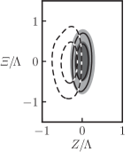
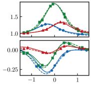
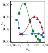
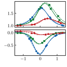
(a) (b)(c)$S_{\!\Lambda}T$$\psi_{\overline{\boldsymbol{q}}}$$\dfrac{A_{\overline{\boldsymbol{q}}}}{\langle A_{\overline{\boldsymbol{q}}}\rangle}$     (d)
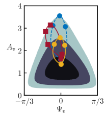
(e) ${A_{\overline{v}}}/{A_{\overline{v}M}}$      (f)(g)$S_{\!\Lambda}T$$\psi_{\overline{\boldsymbol{q}}}$$\dfrac{A_{\overline{\boldsymbol{q}}}}{\langle A_{\overline{\boldsymbol{q}}}\rangle}$

Figure 8: (a) Snapshot of the conditional bursts of $\overline{\boldsymbol{q}}_{2}$ at $S_{\!\Lambda}T=0$, the peaking time of $\overline{v}_{2}$. The contours, normalised with the maximum of each component are: shaded, $A_{\overline{v}}=(0.6,0.8)$; solid $A_{\overline{u}}=(0.8,0.9)$; dashed $A_{\overline{w}}=(0.8,0.9)$. (b–e) Different aspects of the evolution of $A$ and $\Psi$, conditioned to the presence of a burst. F2000. (b) Temporal evolution of the maximum amplitude, as a function of time. , conditional $\overline{u}_{2}$; , conditional $\overline{u}_{3}$. Symbols are , $\overline{u}$; , $\overline{v}$; , $\overline{w}$. (c) As (b), for the deviations of the inclination angle respect to their mean, at the position of the maxima of each component at every instant. (d) Transient amplification of a linearised Orr burst. Conditions are as in figure 1(b), but the energies are computed over the range of $y$ corresponding to the $\Lambda_{2}$ filter. (e) The shaded contours are the joint p.d.f. of $(\Psi_{\overline{v}},A_{\overline{v}})$ for $\Lambda_{2}$. —$\bullet$—, Evolution in (b–c), conditioned to (22); - - $\bullet$ - -, conditioned to the higher threshold (27); —  — evolution in (f–g), conditioned to (28). The five markers are $S_{\!\Lambda}T=[-1.5,-0.3,0,0.3,1.5]$. (f, g) As in (b, c), but conditioned to a burst precursor.

While in the previous section we inferred a hypothetical burst evolution from the statistical relations among the different quantities along the upper edge of the joint p.d.f. of $(\Psi_{\overline{v}},A_{\overline{v}})$, we now turn our attention to the direct study of their conditional temporal evolution by examining structures that pass through the upper ‘tip’ of the joint p.d.f.,

$$A_{{\overline{v}}}>2A_{{\overline{v}}M},\qquad\left|\Psi_{{\overline{v}}}\right|<0.15,$$ (22)

at some stage of their lives. We know from figure 6(e) that the standard deviation of the CMVs passing through these very intense events is low, and that the statistics along the upper edge of the p.d.f. are approximately the same as those of linearised Orr bursts. This suggests that they represent the evolution of individual bursts, at least as long as the amplitude threshold is chosen high enough to separate bursts from each other. The restriction in (22) to a small inclination angle is not strictly necessary, since it follows from figure 6 that intense wall-normal velocity structures are almost always vertical, but including it allows us to relax somewhat the requirement for large amplitudes, and to identify bursts that would be too weak otherwise. The analysis is most easily performed in a convective frame of reference, $(\xi=x-C_{\!\Lambda}t,\,z,t)$ where $C_{\!\Lambda}$ is the convection velocity used in (20). We identify the position and time, $(\xi_{c},z_{c},t_{c})$, of the maximum amplitude for each region as representative of the ‘peaking’ point, $(\xi_{c},z_{c},t_{c})=\text{argmax }{A_{\overline{v}}(\xi,z,t)}$, of the burst, and use it as the centre for our conditionally averaged evolution $\langle\cdot\rangle_{B}$, defined as

$${\langle a\rangle_{B}}(\Xi,Z,T)=\frac{1}{N}\sum_{c=1,...,N}a(\xi_{c}+\Xi,z_{c}+Z,t_{c}+T),$$ (23)

where $N$ is the number of identified bursts for each filter (see table 3), and $a$ is either $A_{{\overline{u}},{\overline{v}},{\overline{w}}}$ or $\Psi_{{\overline{u}},{\overline{v}},{\overline{w}}}$. To avoid ‘false positives’, we discard small bursts for which $\mathcal{S}<2.25\Lambda^{2}$, where $\mathcal{S}$ is the temporally averaged area enclosed in the $(x,z)$ plane by the threshold in (22). Independently of the chosen threshold, approximately 5% of the identified bursts are temporally clustered in quick succession, reminiscent of the ‘packets’ of vortical structures reported by Adrian et al. (2000), but most cases cannot be easily grouped into such packets.

Bursts defined in this way are spatio-temporal objects in $(\xi,z,t)$. To normalise their density per unit duration–area, we assume that two bursts cannot occupy the same volume in space–time, and that they scale spatially with $\Lambda$, and temporally with the inverse of the average shear across their integration band (17),

$$S_{\!\Lambda}=(U(y_{1}(\Lambda))-U(y_{0}(\Lambda)))/(y_{1}(\Lambda)-y_{0}(\Lambda)).$$ (24)

Their expected duration-size would then be proportional to $\Lambda^{2}/S_{\!\Lambda}$, and the number of detected bursts should collapse when their total duration-area is normalised in these units. Table 3 shows that this is approximately true, with a density close to $10\%$ except for the largest filter, which is too large for the scaling to hold. This density is of the same order as the volume fraction of the ‘Q’ structures studied in Lozano-Durán et al. (2012).

Figure 8(a) shows a snapshot of the conditional burst of $\overline{\boldsymbol{q}}_{2}$ in F2000 at peaking time. Other filters collapse well with $\Lambda$, with average dimensions $(\ell_{\Xi}/\Lambda,\ell_{Z}/\Lambda)\approx(2,1)$. The filtered spanwise velocity can be seen to be offset to one side of the streamwise and wall-normal components, while the latter fall on top of each other. If the average had been computed strictly as in (23), the conditional mean evolution would have two symmetric lobes of $A_{\overline{w}}$ centred on the burst, but this symmetry is statistical, and does not imply the symmetry of individual events. The equations of motion and boundary conditions of the channel are invariant to reflections with respect to $(x,y)$ planes, so that any solution $(u(x,y,z),v(x,y,z),w(x,y,z))$ implies that $(u(x,y,-z),v(x,y,-z),-w(x,y,-z))$ is also a solution. Individual Orr events are equally likely to be chiral-left or chiral-right, and the reflection symmetry can be applied to each snapshot to obtain an average that is more representative of individual events (Stretch, 1990; Lozano-Durán et al., 2012). There is no unique way of deciding how to do this consistently for complete histories, and the criterion that we found to produce the least symmetric conditional mean was to always locate to the left of the burst the strongest maximum of $A_{\overline{w}}$ as it passes through the spatio-temporal neighbourhood of its peak:

$$|\Xi|\leq 0.2\Lambda,\,|Z|\leq\Lambda,\,S_{\!\Lambda}|T|\leq 0.2.$$ (25)

The conditional histories computed in this way only contain one region of strong $w$, as in figure 8(a), suggesting that most of the underlying events have only one strong spanwise velocity region, corresponding to a single streamwise roller. Double rollers are found more seldom. Visual inspection of a representative sample of cases shows that approximately 5% of the bursts are almost symmetric, with two $w$ lobes.

Figure 8(b) shows the conditional evolution of the maximum amplitude of the three filtered velocity components as a function of time. Far from $S_{\!\Lambda}T=0$, the three components tend to their unconditional mean, which is used to normalise the plot. The wall-normal velocity, which is used to condition the temporal evolution, is amplified the most, but the streamwise and spanwise velocities are also amplified, peaking at $S_{\!\Lambda}T\approx\pm 0.3$, respectively before and after the peak of $\langle A_{\overline{v}}\rangle_{B}$, as also suggested by figure 7(d, e). The evolution of the deviation of the inclination angles from their unconditional means,

$$\langle\psi_{\overline{a}}\rangle_{B}=\langle\Psi_{\overline{a}}\rangle_{B}-\langle\Psi_{\overline{a}}\rangle,$$ (26)

is presented in figure 8(c), which plots the inclination at the location of the maximum amplitude of each component. The evolution of the inclination angles of the streamwise and wall-normal velocity is from negative to positive, and tends to the unconditional mean beyond $|S_{\!\Lambda}T|\approx 1$. The changes in $\Psi_{\overline{w}}$ are less pronounced, with values closer to its unconditional mean across the whole evolution.

A reference to figure 1 shows that this behaviour is qualitatively similar to linearised equilateral Orr bursts, but there are some interesting differences. The inclination angles of $\overline{u}$ and $\overline{v}$ are proportional to each other in the upper part of the p.d.f. of $(\Psi_{\overline{v}},A_{\overline{v}})$, where the presumed quasi-linear cycle takes place, but the inclination angle of $\overline{w}$ is not. While $\Psi_{\overline{u}}$ evolves from negative to positive in both figures 1 and 7(e), the inclination $\Psi_{\overline{w}}$ is never negative in figures 7(f) and 8(c). Moreover the conditional amplification of $\overline{u}$, as given by the ratio between the highest and lowest conditional averages in figure 7(c), is almost three times higher than that for $\overline{w}$ in figure 7(d), while the opposite seems to be true in figure 1(b), and the maximum amplitudes of the two variables in figure 8(b) are approximately equal. The reason turns out to be the different spatial location of the various velocity components. We saw in figure 8(a) that, while the structures of $\overline{u}$ and $\overline{v}$ are spatially collocated in $(x,z)$, the $\overline{w}$-eddy is offset to one side, resulting in a weaker footprint in the conditional joint p.d.f.s. Even more important is the vertical offset. The amplitudes in figure 1(b) are integrated over the whole channel, but those in figure 7 are band-pass filtered. This includes the wall-parallel filtering by wavelength, which has no effect on the monochromatic wavetrain in figure 1, but also the restriction in (17)–(18) to a band of wall distances, which changes the balance among the different components as they drift vertically in and out of the filtering band. This effect is visually clear from figure 1(a), and figure 8(d) shows that it can be reproduced by restricting the amplitudes in figure 1(b) to the same band of wall distances as in figure 7. It was already mentioned when discussing figure 1 that the definition of the angles is biased by the different amplitude distribution of the three velocity components, and it is now clear that so is the definition of the band-pass amplitudes. Thus, while figures 7(c, d) and 8(b–d) might give the impression that the earlier part of the burst is dominated by the association of $u$ and $v$ (such as in a spanwise-oriented roller), while the later part is dominated by a streamwise roller (of $v$ and $w$), this interpretation could also be an artefact of how the flow is filtered. It should be remembered that linear models cannot change the wall-parallel wavevector of a single mode, nor its wall-parallel orientation, and changes in them have to be attributed to nonlinearity, or to the different amplification of different wavenumbers within a wavepacket, which probably would not apply to the relatively narrow wavebands here. This suggests that the interpretation of the phenomenon as a ‘rotating’ roller outlined above should be disregarded. Nevertheless, figures 8(d) and 1(b) are similar, even though the relative amplitudes of the velocity components are different in both figures due to the energy contained outside the $y$-band limits. Moreover, Jiménez (2013) showed that the cross-correlation of $v$ and $w$, integrated across the channel half-height, has a delayed peak when it is conditioned to a $v$-burst, albeit with slightly different delay between components. These evidences corroborate the causal relation between the burst and the increase in the magnitude of $w$. Other interpretations are also possible. For example, $A_{\overline{w}}$ could also be indicative of streak breakdown, which has been observed in the buffer-layer streaks (Kline et al., 1967; Jiménez & Moin, 1991; Hamilton et al., 1995) or in transient growth modes in the transition of boundary layers in the presence of a streaky background (Brandt & Henningson, 2002).

Figure 8(b) includes results for two different filters, which scale well when normalised with the mean shear (24), and imply lifetimes of the order of $S_{\!\Lambda}T\approx 1$, measured at one-half the maximum amplification. Using slightly different definitions of mean shear and lifetime, Lozano-Durán & Jiménez (2014) and Jiménez (2015) report the somewhat longer value $S_{\!\Lambda}T\approx 5$. In fact, the evolution of the inclination angle in figure 8(c) suggests that the conditional evolution only represents individual bursts when they are relatively near the conditioning time, $S_{\!\Lambda}|T|\lesssim 0.5$, beyond which both the angle and the amplitude tend to their unconditional values.

This is better seen in figure 8(f) which displays the $(\Psi_{\overline{v}},A_{\overline{v}})$ trajectory of figure 8(b, c) on top of the joint $(\Psi_{{\overline{v}}},A_{{\overline{v}}})$ p.d.f.. The trajectory follows the direction of the CMVs near the conditioning point, but soon drops into the high-probability region at the core of the p.d.f.. Note that the trajectory crosses the lowest possible point consistent with (22). Most eddies are in the core of the joint p.d.f., and any conditional mean is dominated by the points closest to the core. In a similar way, once the effect of the condition is lost, trajectories naturally fall towards the probability maximum. Thus, if condition (22) is substituted by the higher-amplitude one,

$$A_{{\overline{v}}}>3A_{{\overline{v}}M},\qquad\left|\Psi_{{\overline{v}}}\right|<0.15,$$ (27)

the conditional trajectory changes to the qualitatively similar, but higher-intensity, trajectory plotted as dashed in figure 8(f).

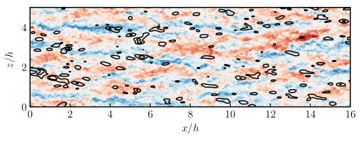
Figure 9: Wall-parallel plane of the streamwise velocity of F2000. The shading is $u^{+}$ at $y/h\approx 0.2$, ranging from $u^{+}\approx-5$ (blue) to $u^{+}\approx 5$ (red). The line contours are $A_{{\overline{u}}_{2}}$ for the same snapshot, representing 50 and 75% of the absolute maximum of $A_{{\overline{u}}_{2}}$ at the plane.

Perhaps the most interesting feature of the conditional evolution is the peak of $\overline{u}$ preceding the burst, also represented by the high values of the conditional amplitude of $\overline{u}$ over the left part of the joint p.d.f. of $(\Psi_{\overline{v}},A_{\overline{v}},)$ in figure 7(c, e). Note that a strong $A_{\overline{u}}$ should not be interpreted as a especially strong streak of the streamwise velocity, because the band-pass filter is designed to capture the energy of $v$, and the structures of $u$ are between six and ten times longer than those of $v$ (Jiménez, 2018). The band-pass-filtered amplitude of a uniform infinite streak is zero, and we should consider $A_{\overline{u}}$ as a measure of the inhomogeneity of the streak, e.g. due to break-up or to ‘meandering’. Streak inhomogeneities have often been identified as important features of the logarithmic layer cycle (Flores & Jiménez, 2010; de Giovanetti et al., 2017). The difference between $u$ and $A_{\overline{u}}$ is illustrated in figure 9, which shows both quantities in a wall-parallel plane of F2000. The streamwise velocity perturbations are shaded at $y/h\approx 0.2$, and the line contours are strong regions of $A_{\overline{u}_{2}}$. It is clear from the figure that both flow features are markedly different, and should not be confused.

The previous discussion shows that a burst of $\overline{v}$ is preceded by backwards-leaning perturbations of $\overline{u}$. The converse, that backwards-leaning perturbations of $\overline{u}$ act as precursors of the bursts of $\overline{v}$, is tested in figure 8(f, g) by the conditional evolution of bursts conditioned to

$$A_{\overline{u}}>1.8A_{{\overline{u}}M},\quad\Psi_{\overline{u}}<-0.4,$$ (28)

which is on the left edge of the joint $(\Psi_{\overline{v}},A_{\overline{v}})$ p.d.f., but relatively far from its top. As shown in the figure, the conditional burst develops as predicted, with qualitatively similar temporal relations and delays among the different components as in figure 8(b, c). It is particularly striking that, even if figure 8(e, f) is conditioned on $\overline{u}$ rather than on $\overline{v}$, the amplification of the latter is even stronger than that of the former, suggesting that at least the left part of the joint p.d.f. represents well-organised bursts. A similar conclusion was reached by Jiménez (2015), who showed that bursts could be linearly ‘predicted’ from conditions up to about half their lifetime before the peak amplification of $v$. The mean trajectory in $(\Psi_{\overline{v}},A_{\overline{v}})$ space of the evolutions initialised within (28) is plotted with squares in figure 8(e). Attempts to use the later peak of $A_{\overline{w}}$ to ‘postdict’ the burst of $\overline{v}$ were not successful. This may be interpreted as that strong, forward-leaning perturbations of $\overline{w}$ are not generated solely by Orr bursts. If this kind of $w$-perturbations can be generated by some other dynamics, denoted in this paragraph as ‘B’, it can only be assured that Orr bursts lead to forward-leaning $w$ perturbations, as well as do ‘B’ events; but identifying forward-leaning $w$ perturbations is not enough to determine if they come from Orr bursts, or from ‘B’ dynamics.

5 Low-pass-filtered velocity fields

We mentioned in §3.2 that, while the band-pass-filtered field (11) is useful in isolating the amplitude and inclination of eddies of a given size, it is not easily interpreted as a velocity. As a consequence, the conditional results in the previous section give only limited information about the flow structure. In particular, the local sign of the velocities is missing, and so is the relation of individual features with the flow around them. Both are important. Sweeps (negative wall-normal velocity events) and ejections (positive wall-normal velocity events) are known to have different characteristics (Lu & Willmarth, 1973; Wallace et al., 1972; Lozano-Durán et al., 2012), and this asymmetry is strongest for the wall-attached structures responsible for most of the tangential Reynolds stress (Dong et al., 2017). Similarly, bursts of the wall-normal velocity are known to be associated with streamwise-velocity streaks (Lozano-Durán et al., 2012; Dong et al., 2017), but the two velocity components have very different sizes. Figure 10(a) shows that the spectrum of $u$ in the logarithmic region is much longer than that of $v$, and it is difficult to study the interaction of the two variables if they are band-passed to a single scale.

Both deficiencies are substantially remedied by the low-pass-filtered velocity (8), which is easily interpreted as a smoothed flow field, and retains the largest features of the flow, including the long streaks of $u$. Unfortunately, these low-passed fields are not approximate wavetrains or wavepackets, and we lose the information about the local inclination angle used in (22) as part of the condition to identify bursts. However, we saw when discussing that condition that the inclination angle was only intended to relax the intensity identification threshold, since figure 6 shows that high amplitudes are unlikely to be anything but vertical. As a consequence, we study in this section conditional flow histories conditioned only on the intensity of the events, and expect their inclination, if any, to emerge as a consequence of that conditioning. Since this requires both a large computational box to contain the largest flow structures, and temporal information, the rest of the section only uses the temporally resolved simulation F2000.

	$\Lambda_{1}$	$\Lambda_{2}$	$\Lambda_{3}$	$\Lambda_{4}$
Number of sweeps	637	2898	17079	147686
Number of ejections	797	3282	18159	160207
Number of pairs	410	1717	9995	82009
Sweeps per time-area in $S_{\!\Lambda}/\Lambda^{2}$	0.118	0.065	0.052	0.06
Ejections per time-area in $S_{\!\Lambda}/\Lambda^{2}$	0.147	0.073	0.055	0.065

Table 4: Number of bursts found in the low-pass-filtered temporal series of F2000. The details of the time-area normalisation are in §4.2.

We create filtered fields using the low-pass filters described in §3.2 and, to obtain structures that are approximately equivalent to the band-passed ones in §4.2, integrate the resulting velocity over the same $y$ bands. The resulting two-dimensional fields recall the amplitudes studied in §4.2, but contain intense regions of negative as well as of positive velocity. Therefore, the process of isolating intense regions of the wall-normal velocity now consists of two independent thresholding operations, $\widetilde{v}_{i}>2\widetilde{v}_{i}^{\prime}$ for ejections, and $\widetilde{v}_{i}<-2\widetilde{v}_{i}^{\prime}$ for sweeps, where $\widetilde{v}_{i}^{\prime}$ is the root-mean-square intensity of the filtered time series. This results in two sets of intense events, which are treated independently, and the rest of the section includes averages conditioned to one or to the other. As a consequence, the presence of a sweep in a flow conditioned to ejections should be considered a feature of the flow, not of the conditioning, and vice versa.

As in §4.2, the purpose of the threshold used to define the sweeps and ejections is mostly to separate individual events, and its value is not critical. We also discard bursts that are too small, and, in addition, merge into a single object bursts of the same sign whose centres, $(\xi_{c},z_{c},t_{c})$, defined as the location of their maximum intensity, are too close to each other. The centre of the resulting object is taken to be the centre of the stronger of the two eddies being merged. We saw in §4.2 that the size of the bursts is $\ell_{\Xi}/\Lambda\sim\ell_{Z}/\Lambda\sim Tu_{\tau}/\Lambda\sim O(1)$, and, after some experimentation, choose as the merging criterion that

$$\sqrt{(\rmDelta t_{c}u_{\tau})^{2}+(\rmDelta\xi_{c})^{2}+(\rmDelta z_{c})^{2}}<0.15\Lambda.$$ (29)

The number of centres determined in this way is given in table 4 for each filter size. Centring each burst on its defining extremum, the conditional structures are computed as in (23), using the four-dimensional filtered histories without integrating them in $y$, to retain the wall-normal burst structure:

$${\langle a\rangle_{L}}(\Xi,y,Z,T)=\frac{1}{N}\sum_{c=1,...,N}a(\xi_{c}+\Xi,y,z_{c}+Z,t_{c}+T).$$ (30)

For each burst, we use a centred four-dimensional box spanning the channel half-height, $y=(0,h)$, the wall-parallel box with dimensions $\Xi/h\!=\!\pm 4\pi,\,Z/\Lambda\!=\!\pm 3$, and a time interval consistent with the burst lifetimes discussed in §4.2, $S_{\!\Lambda}T\!\approx\!\pm 5$. The conditional mean evolutions for the different filters are found to collapse spatially when normalised with the height of the most intense point of the conditional evolution, $y_{c}$, which can be interpreted as the distance from the wall of the centre of the conditional burst at the moment of its highest intensity. Figure 10(b) shows that $y_{c}$ increases linearly with the filter width as $y_{c}^{+}=\Lambda^{+}/2+100$, corresponding to bursts whose central height is proportional to $\Lambda/2$, with an offset of $100\nu/u_{\tau}$ representing the buffer layer. Because of this offset, the spatial structure of the bursts collapses better with $y_{c}$ than with $\Lambda$, and this scaling will be used in the rest of the section.

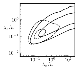
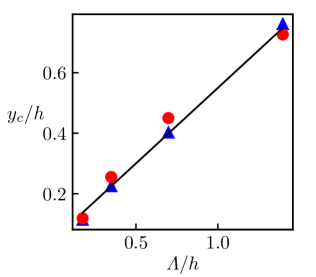
(a)       (b)

Figure 10: (a) Spectra of:   , the streamwise velocity; , the wall-normal velocity, integrated over $y/h\in[0.2,0.4]$. Contours contain 50% and 10% of the integrated spectral mass. (b) Distance from the wall of the point of highest intensity of the conditional burst. ejections; sweeps. The diagonal line is $y_{c}/h=0.5\Lambda/h+0.05$.

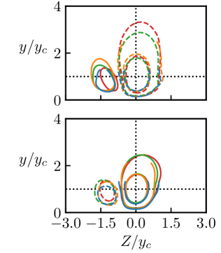
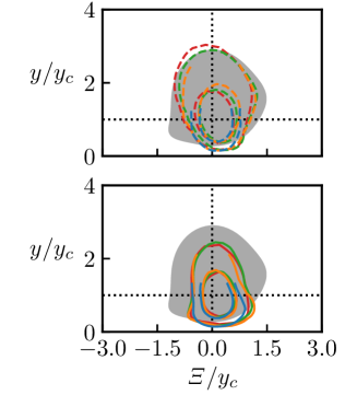
(a)sweepejection       (b)sweepejection

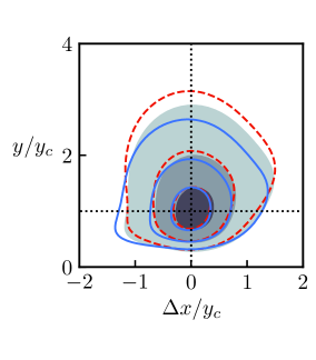
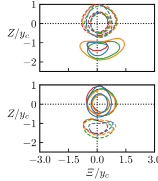
.   (c)        (d)sweepejection

Figure 11: (a, b, d) Different sections of the conditional structure of $\widetilde{v}$ at the peak of the $v$-burst, $S_{\!\Lambda}T=0$, for the four filters. F2000.   , positive wall-normal velocity; , negative. The contours are (-0.15, 0.15, .45) of the corresponding extremum. In each figure the top panel is conditioned to the sweep, and the bottom one, to the ejection. The lines are: blue, $\widetilde{v}_{1}$; orange, $\widetilde{v}_{2}$; green, $\widetilde{v}_{3}$; red, $\widetilde{v}_{4}$. (c) Autocorrelation function of the wall normal velocity, $C_{vv}(\rmDelta x,y,y^{\prime})$ at $y^{\prime}=0.05h=100\nu/u_{\tau}$. The shaded contours are the unconditional autocorrelation function;   , autocorrelation only for positive $v$ events; , autocorrelation only for negative $v$ events. Contours are (0.15, 0.3, 0.6) of the maximum correlation in each case.

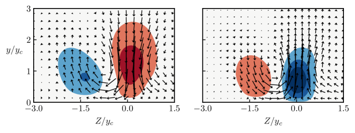
(a)(b)

Figure 12: $(y,Z)-$section of the conditional mean structure of $\widetilde{\boldsymbol{q}}_{2}$ at the peak of the $v$-burst, $S_{\!\Lambda}T\!=\!0$. F2000. The shaded contours are streamwise velocity perturbations, $\widetilde{u}_{2}^{+}=\pm(0.5,0.9,1.3)$. The arrows are the cross-plane velocities, with values in $(\widetilde{v}_{2}^{2}+\widetilde{w}_{2}^{2})^{1/2}=[0,u_{\tau}]$, represented by the arrow length. (a) Conditional sweep. (b) Conditional ejection.

Figure 11 provides three orthogonal sections of the three-dimensional structure of the bursts at $S_{\!\Lambda}T=0$, and shows that the scaling with $y_{c}$ is extremely good, only interrupted by the channel centreline. The largest filters produce ‘cropped’ bursts at $y=h$, but they agree well below that height. The dotted lines in each figure show the location of the other two sections. Individual ejections and sweeps are often accompanied by a single strong structure with opposite wall-normal velocity (Lozano-Durán et al., 2012), sitting at $\Xi\approx 0,\,Z/y_{c}\approx\pm 1.2$. Inspection of a representative sample of individual bursts shows that only about $5\%$ of them have more than one companion, and are approximately symmetric. As in §4.2, the bursts in (30) are oriented to retain as much as possible the asymmetry of this arrangement in the conditional mean. This is done by placing on a negative $Z$ the strongest ejection found in the neighbourhood

$$|\Xi|\leq 0.2\Lambda,\,|Z|\leq\Lambda.$$ (31)

of the conditioning sweep (or vice versa), reflecting the velocity field as required. For all the filters and conditions tested, the companion appears in the conditional evolution as a single opposite-signed ‘partner’ with half the intensity of the main structure.

Small differences can be seen between the conditional sweeps and the ejections. For example, the ejections in the bottom panel of figure 11(b) have small upstream $(\Xi<0)$ ‘tails’ near the wall, while the sweeps in the upper panel have a more rounded downstream ‘nose’ farther from the wall. Interestingly, both features are also found in the autocorrelation function of the wall-normal velocity, added to figure 11(b) as a shaded area, suggesting that different regions of the autocorrelation function of the wall-normal velocity are controlled by perturbations of different sign.

A similar effect was found by Sillero et al. (2014) for the $(x,z)$ sections of the autocorrelation of the spanwise velocity. They found them to be approximately square, and showed that, when the correlation is conditioned to only positive or negative values of $w$ at the reference point, the correlation separates into two almost diagonal patterns, which form the square when added together. Here, sweeps and ejections contribute to the ‘nose’ and ‘tail’ of the unconditional correlation of $v$, respectively. This is confirmed in figure 11(c) which shows the autocorrelation functions of $v$ at $y/h\approx 0.05$:

$$C_{vv}(\rmDelta x,y,y^{\prime}=0.05h)=\langle v(x+\rmDelta x,y)v(x,y^{\prime}=0.05h)\rangle,$$ (32)

where the average $\langle\cdot\rangle$ is performed in three different ways: unconditionally (shaded in the figure), and conditioned to either negative (dashed lines) or positive (solid lines) values of $v$ at the reference point $v(x,0.05h)$.

Figure 11(d) shows that the wall-parallel sections of the conditioning burst are roughly circular, whereas the conditional partners are bean-shaped, but we will show in §5.1 that the mismatch between the shapes of the bursts and of their partners is almost surely an artefact of the conditional average, not of the instantaneous flow fields.

Figure 12 shows a cross-flow section of the conditional $\widetilde{\boldsymbol{q}}_{2}$ field. The figure is conditioned on $v$, and the shaded contours are streamwise velocity perturbations. The sign of the primary $u$ structure (near $Z=0$) is opposite to the one of $v$, forming a classical $(\mathrm{Q}_{2},\,u<0,v>0)$ or $(\mathrm{Q}_{4},\,u>0,v<0)$ eddy. Both cases have a weaker partner of opposite polarity at $Z/y_{c}\approx-1.2$, and the complete structure shares many features with the conditional pairs of $uv$-$\mathrm{Q}$s in Lozano-Durán et al. (2012) and Dong et al. (2017), which were conditioned on their intensity, without regard to their temporal evolution. Those authors found that strong $\mathrm{Q}$s can be classified as ‘attached’, with roots that extend very near the wall, or ‘detached’, which do not. The attached $\mathrm{Q}$s are self-similar, as in the present case, form $\mathrm{Q}_{2}$–$\mathrm{Q}_{4}$ pairs of size comparable to the present ones and, when conditionally averaged by centring them on the centre of gravity of the pair, they also contain a roller between streaks. They are responsible for most of the tangential Reynolds stress in the flow. Similar rollers have been identified as part of the self-sustaining cycle of the buffer layer, where they tend to be almost parallel to the wall (Jiménez & Moin, 1991; Hamilton et al., 1995; Jiménez & Pinelli, 1999; Schoppa & Hussain, 2002; Jiménez et al., 2005), and are also believed to be important in the logarithmic layer (Flores & Jiménez, 2010; de Giovanetti et al., 2017). In our case, the roller remains inclined in the $(\Xi,y)$ plane at approximately 15^o during the evolution (not shown), sitting between the pair of streaks. This is similar to the inclinations previously found from the autocorrelation of $u$ (see Sillero et al., 2014, for a review). The similarity between all these structures suggests that bursts, Qs and quasi-streamwise vortices are different manifestations of the same phenomenon.

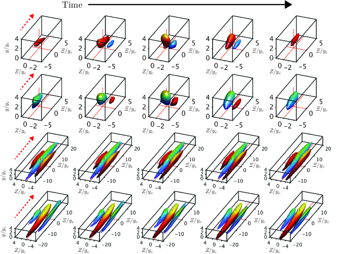
(a)(b)(c)(d)

Figure 13: Mean evolution of $\widetilde{v}_{2}$ and $\widetilde{u}_{2}$ conditioned to the presence of a burst in F2000. The snapshots range from $S_{\!\Lambda}T=-4(2)4$. The flow moves in the direction of the dashed arrow, an the mean advection between snapshots has been removed. (a, b) The blue surface corresponds to $\widetilde{v}_{2}^{+}<-0.15$ and the red to $\widetilde{v}_{2}^{+}>0.15$. (a) Conditioned to a sweep. (b) Conditioned to an ejection. (c, d) As in (a, b), but for the evolution of $\widetilde{u}_{2}$; the surfaces are, blue, $\widetilde{u}_{2}^{+}<-0.15$; red, $\widetilde{u}_{2}^{+}>0.15$.

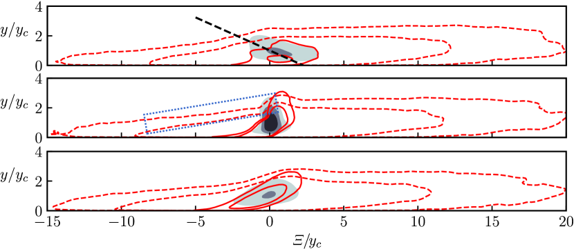
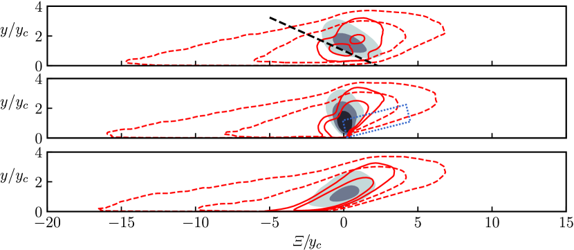
(a)(b)(c) (d)(e)(f)

Figure 14: (a–c) $Z=0$ section of the low-passed-filtered low-speed streak (dashed lines, $|\tilde{u}_{2}^{+}|=[0.15,0.3]$) and its associated ejection (shaded contours, $|\tilde{v}_{2}^{+}|=[0.15,0.3,0.6]$). The solid lines are the shorter wavelengths of the filtered streamwise velocity, comparable to the band-pass-filtered velocity in §4, as explained in the text. (a) $S_{\!\Lambda}T=-2$. (b) $S_{\!\Lambda}T=0$. (c) $S_{\!\Lambda}T=2$. (d–f) As in (a–c), but for the high-speed streak, and the wall-normal velocity sweep. F2000.

Up to now, we have described bursts at the moment of their maximum intensity, but figures 13(a) and 13(b) show the time evolution of a constant isosurface of $\widetilde{v}_{2}$ for the conditional evolution of an ejection and a sweep, respectively. The burst is always located at $Z/y_{c}\approx 0$, and its partner structure at $Z/y_{c}\approx-1.2$, as in figure 11(d). The conditional evolution spans a total of $S_{\!\Lambda}T=8$, clearly showing an Orr-like evolution of the inclination angle and amplitude of the burst in both cases. The partner structure is present during the full evolution, and is amplified by approximately the same amount as the conditioning burst, but with half its average intensity. Figure 13(c, d) shows the evolution of the streamwise velocity streaks during the same conditional event. They are considerably longer ($\sim 20y_{c}$) than the $v$-bursts ($\sim 3y_{c}$) and, unlike the latter, which have a single secondary lateral structure, they have a pair of comparable streaks of the opposite sign at each side. However, although there is some amplification of the streak during the burst, evidenced in the figure by the thickening and lengthening of their $u$ isosurface, it is less clear than the amplification of $v$. In particular, the streaks are already present in the conditioning volume when the $v$-burst begins to form, and remain in it when the burst disappears. The alternating pattern of streaks contains a maximum in the magnitude of the spanwise variation of the streamwise velocity, $\partial\tilde{u}/\partial z$, located within the pair of bursts. This local extrema of the spanwise variation could be a marker of the sinous instability of the streamwise streaks, reminiscent of the dynamics of the buffer-layer streaks analysed by other authors (Hamilton et al., 1995; Waleffe, 1997). However, it should be considered that the conditional structure is strongly affected by the correlation of the wall-normal velocity with the rest of the flow, and thus the local maxima of $\partial\tilde{u}/\partial z$ observed in the conditional eddy could be an effect of the correlation of the spanwise derivative with $v$.

Figure 14 shows longitudinal $Z=0$ sections of the conditional evolutions in figure 13, at different moments during the burst. To be able to compare it with the band-pass-filtered conditional evolution in §4.2, we also provide contours of the band-pass-filtered streamwise velocity, obtained by filtering the conditional field (which already is an average of low-pass-filtered fields) with a high-pass filter chosen so that the scales retained by the combined effect of the two filters are comparable to the band-pass filter in §4. Filtering the streamwise velocity in this way reveals an inner ‘core’ of the streak. While the longer ‘body’ of the streak is always tilted forwards, the much shorter core tilts both backwards and forwards in synchrony with the wall-normal velocity. This confirms the different nature of the short (band-pass-filtered) and long (low-pass-filtered) perturbations of the streamwise velocity discussed in §4. It is worth noting that the sweep is located towards the front of the high-speed streak, whereas the ejection tends to be closer to the back of the low-speed streak, recalling a similar arrangement of streaks and vortices in the buffer layer (see figure 9b in Jiménez et al., 2004).

Before interpreting these results, it is important to understand that figures 13(c, d) and 14 do not represent instantaneous streaks, or even averaged ones, but the part of the streak conditioned to the presence of a strong burst of $v$. As such, the intensity of the structures in those figures reflects both the intensity of the fluctuations of $u$, and how is $u$ correlated to the burst. For example, the isolines in figure 14 do not represent the intensity of $u$, and can not be used to estimate that intensity except probably near the inner core. Any attempt to derive from them whether the burst is a consequence of the presence of the streak, or the other way around, is bound to be speculative. In the same way, the fact that the streaks in figure 13(c, d) are not seen to strengthen during the burst does not mean that they do not do so (or vice versa).

With these restrictions in mind, the simplest interpretation of the positional bias in figure 14 is that the streaks are ‘wakes’ created by sweeps and ejections advected by the mean flow at the wall-distance at which they originate (Jiménez et al., 2004). Sweeps, coming from above, move faster than the local mean speed and bring high-speed fluid down, leaving a high-speed wake upstream. The effect of the ejections is the opposite. However, it was argued by del Álamo et al. (2006) that this explanation is unlikely, because the $v$-bursts do not live long enough. Thus, if we take their lifetime to be the same as for Qs, $T^{+}\approx 2y_{c}^{+}$ and the velocity difference to be $O(1.5u_{\tau})$ (Lozano-Durán & Jiménez, 2014), the maximum length of their wake would be $O(3y_{c})$. This is the length of the inner core in figure 14, but much shorter than the length of the streak. A more likely possibility is that each streak is created by several bursts, each of which contributes a small fraction to its length (del Álamo et al., 2006). The fact that the conditional streaks weaken so little away from the peak of the burst in figure 13(c, d) also strongly suggests that the streaks are stable features of the flow, while the burst grows and eventually disappears within them. This is supported by the known streamwise distance between consecutive $\mathrm{Q}$s, $\rmDelta x\approx 7y_{c}$ (Lozano-Durán et al., 2012; Dong et al., 2017), which is much shorter than the streak length. These dimensions will be confirmed for the bursts in the next section.

In fact, if we accept the argument above that very long wakes cannot be a consequence of short-lived bursts, the scaling of figure 14 with the filter width can be used to extract some causal information. We saw in discussing figure 11 that the size on the $v$-burst is proportional to $y_{c}\propto\Lambda$. The inner core of the streak in 14 also scales with $\Lambda$, which is not surprising because it is created by a pseudo-band-pass filter of that size. The causal information is contained in the scaling of the rest of the streak, which is obtained with a low-pass filter, and therefore contains all the scales larger than $\Lambda$. Although not shown in the figure to avoid clutter, most of the streak dimensions scale with $h$, not with $\Lambda$, suggesting that most of the streak it is not caused by the burst, nor does directly causes it. The only regions that scale with $\Lambda$ are the upper edge of the leftward tail of the low-speed streak in figure 14(a–c), and the underside of the rightward nose of the high-speed streak in figure 14(d–f). Both regions are approximately indicated by a dotted rectangle in figure 14(b, e) , and shown for the filters $\Lambda_{2}$–$\Lambda_{4}$ in figure 15, which scales the high-speed and low-speed streaks with $y_{c}$.

We may now come back to the question of what causes the positional bias in figure 14, which is part of the wider question of what causes sweeps and ejections to be organised along streaks. It is generally accepted that wall-normal velocity perturbations create streaks by deforming the mean profile. However, the typical intense $v$-structure, i.e. an Orr burst, is much shorter than the streak, and it is clear from the discussion in the previous paragraphs that it implies that something else organises the bursts so that the short streak segments join into longer objects. The possibility that streak instability is responsible for the bursts has been mentioned often, although the detailed mechanism is unclear (see discussions in Schoppa & Hussain, 2002; Farrell & Ioannou, 2012), as well as the possibility that long streaks are compound objects (Jiménez, 2018). However, most of these analyses deal with infinite uniform streaks, and cannot explain a preferential longitudinal distribution of the bursts within them. Although the question of which are the original perturbations that give rise to the formation of bursts, is beyond the scope of the present paper, an obvious suggestion of the above observations is that bursts are preferentially created at the ‘active’ end, i.e. where the burst is located. This is the same location where the streak ‘collides’ with the ambient flow, either where the upper surface of the back of the slow streaks, is overrun by the faster flow behind, or where the bottom of the ‘nose’ of the faster streak overruns the slower flow ahead. This is justified if we consider that it is only these edges that scale with $y_{c}$, and thus can be affected by the bursts. The rear and upper parts of the high-speed streaks scale better with $h$, and so do the front parts of the low-speed streaks. The dynamics affecting this parts should in principle be independent of the bursts. A somewhat similar distribution of active regions was observed by Abe et al. (2004), who studied the relation of the large-scale structures in channels with the stresses at the wall. The sweeps were found to be related to the part of the high-speed streaks that had a footprint of intense spanwise shear at the wall, this being the ‘active’ part.

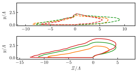
(a)(b)

Figure 15: $Z=0$ section of the low-passed-filtered streamwise velocity streaks ($|\tilde{u}_{2}^{+}|=[0.3]$) for F2000. Lines are: (orange), $\Lambda_{2}$; (green) $\Lambda_{3}$; (red), $\Lambda_{4}$. (a) Low-speed streaks. (b) High-speed streaks.

A slightly different interpretation of the same data is that the streak interaction does not take place at the end of a streak, but in the front of a meander in which high-speed flow pushes into a low-speed one. The conditional data in figure 14 are not enough to distinguish between those two possibilities, even when inspected in other flow sections or in three-dimensional views, and all that can probably be said is that bursts tend to be created at preexisting longitudinal inhomogeneities of the streaks.

5.1 Space–time organisation of sweeps and ejections

It remains unclear from the previous discussion whether the secondary $v$ structure that appears to one side of the conditioning burst in figures 11 and 13(a, b) is an independent Orr burst, a true companion of the conditioning burst, or another unrelated structure. However, it seems unlikely that $v$ ‘monopoles’ of any given sign, strong enough to be reflected in the conditional average, appear isolated in the flow, because continuity requires that the mean wall-normal velocity over patches of dimensions comparable to the distance from the wall should vanish. Our baseline hypothesis, motivated in part by the similarity of the conditional averages in figure 11 to the conditional Qs in Lozano-Durán et al. (2012) and Lozano-Durán & Jiménez (2014), is that bursts appear in side-by-side pairs of opposite sign, and that the secondary structure in figures 11 and 13 is just a poorly centred reflection of the opposite-signed partner of the burst being used to condition the evolution.

  

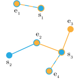
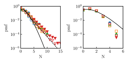
(a)(b)(c)

Figure 16: Probability mass functions (pmfs) of the number of partners of each structure. (a) Sketch of the definitions of pair, partner and number of partners (node degree). (b) Pmf of the number of sweep-partners for ejections (open symbols) and ejection-partners for sweeps (closed symbols). (c) Pmf of the number of ejection-ejection partners (open symbols) and sweep-sweep partners (closed). (a–b) , $\Lambda_{1}$; , $\Lambda_{2}$; , $\Lambda_{3}$; , $\Lambda_{4}$. The solid line is the corresponding distribution for a Poisson process.

To verify this, we compute the distance between the centres of each detected sweep and its closest ejection, and vice versa, defined in the mean-convective frame of reference:

$$L_{2}=\left[(\rmDelta tu_{\tau})^{2}+(\rmDelta z)^{2}+(\rmDelta\xi)^{2}\right]^{1/2}.$$ (33)

Lozano-Durán et al. (2012) and Dong et al. (2017) give similar statistics for unconditional Qs, although without the inclusion of the time difference. In their case, they require restrictions on the relative size of the eddies to avoid pairs with very different components, but this is made unnecessary in our case by only considering structures obtained with a particular filter. The definition of a pair is not straightforward, and figure 16(a) shows a two-dimensional sketch of possible complications. Each sweep, such as s₁, chooses as partner its closest ejection, such as e₁, and may in turn be chosen as partner by other ejections. Partnership is not symmetric. A given sweep may be chosen as partner by several ejections, such as e₂–e₄ in the case of s₃, and each of those may or may not be the ejection chosen by the sweep as its closest partner. Couples which choose each other are defined as pairs, such as (e₁, s₁) and (s₃, e₄) in figure 16(a), and this relation is mutual and unique. Each structure can be part of a pair, or of none at all, but being paired does not preclude having been chosen as a partner by other structures. Examples of unpaired structures are e₂, e₃ and s₂, which have not been chosen by their preferred partner, and a paired structure with a large number of partners (or node degree, in graph notation) is s₃. Approximately 60% of the sweeps are in pairs, and 14% of them are in exclusive pairs (see table 4).

There are no obvious statistical differences between the components of exclusive and non-exclusive pairs, but pairs are not random occurrences. The probability distribution of the degree of the sweeps and ejections is shown in figure 16(b), where it is compared with the expected density function for Poisson-distributed structures, represented by the solid line. It is clear that sweeps and ejections are clustered in the sense of having a higher number of partners of the opposite type than the Poisson model, obtained by randomising the position of the structures. On the other hand, figure 16(c), shows the distribution of the degree of structures of the same type, which is considerably steeper than that for the Poisson process. These two behaviours can be informally summarised as that bursts of opposite type ‘attract’ each other, while those of the same sign ‘repel’, and can probably be explained by the aforementioned effect of continuity, which requires that the net wall-normal mass flux over large areas should tend to vanish.

It is interesting that the probability of having $N>3$ partners of the opposite type in figure 16(b) follows quite closely a geometric distribution $P(N)\sim q^{N}$ with $q=0.4$, represented by the dashed line. This is intriguing, because it implies that the probability of being chosen as a partner is independent of how many partners a structure already has, probably implying that some structures have to choose a distant partner because they cannot find a closer one. This, in turn, suggests that bursts that are not part of a local pair are relatively isolated from prospective partners of the opposite sign. The same is not true for the same-sign partners in figure 16(c) which do not have an exponential tail or, if they do, it is one with a much smaller parameter than in the previous case $(q\approx 0.04)$. The default model proposed by Lozano-Durán et al. (2012) from the analysis of the $uv$ Qs, is that Qs tend to cluster into streamwise trains of tight pairs. The previous discussion suggests that the organisation into trains is better developed than the one in pairs, or at least that many pairs are asymmetric, with one of the partners too weak to be identified as such by the analysis.

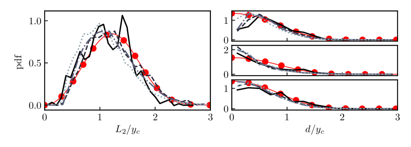
(a)(b)(c)(d) (e)(f)(g)(h)

Figure 17: (a–d) Probability density functions of the distance between components of sweep-ejection pairs. (e–h) Same for sweep-sweep pairs. (a, e) p.d.f. of the space-time distance $L_{2}$, defined in (33). (b, f) p.d.f. of $|\rmDelta tu_{\tau}/y_{c}|$. (c, g) $|\rmDelta z/y_{c}|$. (d, h) $|\rmDelta\xi/y_{c}|$. In all cases, lines are: , $\Lambda_{1}$; , $\Lambda_{2}$; , $\Lambda_{3}$; , $\Lambda_{4}$;    $\bullet$   , p.d.f. of the intra-pair distance for an equivalent Poisson process.

Figure 17 shows the probability distribution of the distance between the components of established pairs, compared with its Poisson counterpart. Figure 17(a–d) refers to sweep–ejection pairs, and figure 17(e–h) to pairs of the same type. More than 90% of the normalised distance between sweeps and ejections fall within $L_{2}/y_{c}\in(0.5,2)$, with its mode at $L_{2}/y_{c}\approx 1.1$. Its p.d.f. is significantly different from the Poisson distribution, shown in the figure as a line with filled circles. Figure 17(b–d) shows the contributions to $L_{2}$ of its different components. The main one is from the spanwise distance, which peaks at approximately $\rmDelta z/y_{c}\approx 1$, similar to the spanwise offset between the main and secondary eddies in figures 11 and 13. The streamwise component also plateaus for $\rmDelta\xi/y_{c}\lesssim 1$, but the temporal offset peaks for contemporaneous events $(\rmDelta t=0)$ and decays quickly. As with the total $L_{2}$ distance, the Poisson model fails for all components. Events tend to be spatially farther from each other than those for the Poisson model, but closer in the time of their peak development. The former is most probably due to the finite size of the objects being considered. Figure 11 shows that the $(x,z)$ diameter of the sweeps and ejections is approximately $y_{c}$, and it is not surprising that there are few pairs in figure 17 spatially closer than that distance. On the other hand, this restriction does not apply to time, and figure 17(b) shows that pairs preferentially evolve in synchrony, as in figure 13.

Figure 17(e–h) tells a slightly different story about homogeneous pairs. In the first place, although the average distances are approximately the same, the homogeneous pairs do not show the same probability deficit at short distances as in the heterogeneous case. Sweeps are closer to each other than their size would appear to allow. The reason can be understood from the individual p.d.f.s in figure 17(f–h). While the exclusion in dissimilar pairs takes place in space, similar pairs are mainly spaced in time. The p.d.f. for $\rmDelta z$ peaks at the origin, in agreement with the model of a train of aligned pairs, and $\rmDelta\xi$ is also only weakly constrained at short distances, but these events do not happen simultaneously, and figure 17(f) reveals a clear deficit for $\rmDelta tu_{\tau}/y_{c}\lesssim 0.5$, or $S\rmDelta t\lesssim 2$. This is of the order of the lifetime of the burst, suggesting that, although consecutive pairs may align along streaks, they are created asynchronously, so that neighbouring sweeps are typically at different stages of their life. Note that this would be consistent with the observation in figure 14 that sweeps tend to form at the ‘active’ front of the streak, and suggests a model in which the trains of bursts propagate incrementally while they extend the streak length. Although it has to be emphasised that, as we have mentioned several times in this discussion, these bursts are only very seldom symmetric hairpins, one cannot avoid noting the similarities between this propagation model and the incremental formation of hairpin packets analysed by Zhou et al. (1999) in the absence of turbulent background activity.

6 Conclusions

Using wavelets as band-pass filters, we have extended the identification in Jiménez (2015) of Orr-like bursts in minimal channel flows, to computational boxes of arbitrary size. Wavelets allow us to reduce the flow to a field of local single-scale wavetrains whose inclination and intensity can be computed, but lack the connection with the surrounding flow and the multiscale character of turbulence. We have complemented this analysis with low-pass filters that retain the very large motions of the streamwise velocity. The evolution of both filtered velocities is tracked in time. Regardless of the filter used, we find significant statistical evidence of Orr-like evolution of localised structures with strong wall-normal velocity.

The intense wall-normal velocity wavefronts are always vertical, and are consistently preceded by backwards-leaning perturbations. The length and time scales of these wavetrains are self-similar with respect to the filter width, especially in the logarithmic layer. Increasing the Reynolds number in the range $Re_{\tau}=950$–4000 simply increases the range of scales in the logarithmic region, resulting in a wider hierarchy of self-similar eddies. When normalised with their filter width, the events have roughly constant duration-a-rea, approximately filling 10% of the time–area at a given height.

We also study the effect of the box size, using short boxes of dimensions $2\pi h\times 2h\times\pi h$, long ones of $8\pi h\times 2h\times 3\pi h$, and comparisons with the single-mode analysis in minimal boxes by Jiménez (2015). We find good agreement between the three box sizes, suggesting that the dynamics of the Orr-like bursts is well captured in minimal domains. The similarities with Jiménez (2015) imply that further studies of the bursting process or related dynamics could be carried using smaller, more affordable simulations. The evolution of the inclination angle and amplitude of the wavefronts of the three velocity components is reasonably well predicted by linearised optimal transient growth, corroborating that the evolution of these events is dominated by linear dynamics.

Because the statistical analysis of the wavetrains shows that the most intense events of the wall-normal velocity are always vertical, Orr events can be identified solely from the amplitude, allowing low-pass filters to identify Orr events while retaining the large-scale motions and the sign of the velocity perturbations. The result is that sweeps and ejections tend to form contemporaneous ‘pairs’, i.e. the peaking of the sweep and of the ejection happens at the same time. The components of the pairs are roughly aligned in the spanwise direction, forming streamwise-oriented tilted rollers, and the rollers tend to be aligned in the streamwise direction with respect to one another. However, rollers tend not to be contemporaneous, and the temporal offset among contiguous rollers is comparable to their lifespan. Sweeps and ejections are embedded in streamwise-velocity streaks of the opposite velocity sign, thus generating negative tangential Reynolds stresses that reinforce the streaks in which they reside. In fact, the evidence from the conditional flow histories in the space–time neighbourhood of strong bursts is that bursts tend to form along preexisting streaks, especially near streamwise streak inhomogeneities.

The characteristics of the Orr events, such as their size, time scale, shape and spatio-temporal organisation, are consistent with the attached three-dimensional regions of intense tangential Reynolds stress studied in (Lozano-Durán et al., 2012; Lozano-Durán & Jiménez, 2014; Dong et al., 2017). These works provide strong indications that the mean shear controls the dynamics of the attached momentum-carrying structures. The new evidence corroborates these findings, suggesting that the ‘tall’ attached momentum-transfer structures are Orr bursts, and can thus be reasonably well described by linear dynamics.

References

- Abe et al. (2018) Abe, H., Antonia, R. A. & Toh, S. 2018 Large-scale structures in a turbulent channel flow with a minimal streamwise flow unit. J. Fluid Mech. 850, 733–768.
- Abe et al. (2004) Abe, H., Kawamura, H. & Choi, H. 2004 Very large-scale structures and their effects on the wall shear-stress fluctuations in a turbulent channel flow up to re = 640. J. Fluids Eng. 126 (5), 835–843.
- Adrian (2007) Adrian, R. J. 2007 Hairpin vortex organization in wall turbulence. Phys. Fluids 19 (4), 041301.
- Adrian et al. (2000) Adrian, R. J., Meinhart, C. D. & Tomkins, C. D. 2000 Vortex organization in the outer region of the turbulent boundary layer. J. Fluid Mech. 422, 1–54.
- del Álamo & Jiménez (2006) del Álamo, J. C. & Jiménez, J. 2006 Linear energy amplification in turbulent channels. J. Fluid Mech. 559, 205–213.
- del Álamo et al. (2004) del Álamo, J. C., Jiménez, J., Zandonade, P. & Moser, R. D. 2004 Scaling of the energy spectra in turbulent channels. J. Fluid Mech. 500, 135–144.
- del Álamo et al. (2006) del Álamo, J. C., Jiménez, J., Zandonade, P. & Moser, R. D. 2006 Self-similar vortex clusters in the logarithmic region. J. Fluid Mech. 561, 329–358.
- Brandt & Henningson (2002) Brandt, L. & Henningson, D. S. 2002 Transition of streamwise streaks in zero-pressure-gradient boundary layers. J. Fluid Mech. 472, 229–261.
- Brown & Roshko (1974) Brown, G. L. & Roshko, A. 1974 On density effects and large structure in turbulent mixing layers. J. Fluid Mech. 64, 775–816.
- Butler & Farrell (1992) Butler, K. M. & Farrell, B. F. 1992 Three-dimensional optimal perturbations in viscous shear flow. Phys. Fluids A: Fluid Dynamics 4 (8), 1637–1650.
- Canuto et al. (1988) Canuto, C., Hussaini, M. Y., Quarteroni, A. & Zang, T. A. 1988 Spectral Methods in Fluid Dynamics. Springer-Verlag, Heidelberg.
- Cess (1958) Cess, R. D. 1958 A survey of the literature on heat transfer in turbulent tube flow. Westinghouse Research Rep. pp. no. 8–0529–R24.
- Dong et al. (2017) Dong, S., Lozano-Durán, A., Sekimoto, A. & Jiménez, J. 2017 Coherent structures in statistically stationary homogeneous shear turbulence. J. Fluid Mech. 816, 167–208.
- Farge (1992) Farge, M. 1992 Wavelet transforms and their applications to turbulence. Annu. rev. fluid mech. 24 (1), 395–458.
- Farrell & Ioannou (1993) Farrell, B. F. & Ioannou, P. J. 1993 Optimal excitation of three-dimensional perturbations in viscous constant shear flow. Phys. Fluids A: Fluid Dynamics 5 (6), 1390–1400.
- Farrell & Ioannou (2012) Farrell, B. F. & Ioannou, P. J. 2012 Dynamics of streamwise rolls and streaks in turbulent wall-bounded shear flow. J. Fluid Mech. 708, 149–196.
- Flores & Jiménez (2006) Flores, O. & Jiménez, J. 2006 Effect of wall-boundary disturbances on turbulent channel flows. J. Fluid Mech. 566, 357–376.
- Flores & Jiménez (2010) Flores, O. & Jiménez, J. 2010 Hierarchy of minimal flow units in the logarithmic layer. Phys. Fluids 22 (7), 071704.
- de Giovanetti et al. (2017) de Giovanetti, M., Sung, H. J. & Hwang, Y. 2017 Streak instability in turbulent channel flow: the seeding mechanism of large-scale motions. J. Fluid Mech. 832, 483–513.
- Hamilton et al. (1995) Hamilton, J. M., Kim, J. & Waleffe, F. 1995 Regeneration mechanisms of near-wall turbulence structures. J. Fluid Mech. 287, 317–348.
- Hoyas & Jiménez (2006) Hoyas, S. & Jiménez, J. 2006 Scaling of the velocity fluctuations in turbulent channels up to . Phys. Fluids 18 (1), 011702.
- Hwang & Cossu (2010) Hwang, Y. & Cossu, C. 2010 Linear non-normal energy amplification of harmonic and stochastic forcing in the turbulent channel flow. J. Fluid Mech. 664, 51–73.
- Jiménez (2013) Jiménez, J. 2013 How linear is wall-bounded turbulence? Phys. Fluids 25 (11), 110814.
- Jiménez (2015) Jiménez, J. 2015 Direct detection of linearized bursts in turbulence. Phys. Fluids 27 (6), 065102.
- Jiménez (2018) Jiménez, J. 2018 Coherent structures in wall-bounded turbulence. J. Fluid Mech. 842, 1.
- Jiménez et al. (2004) Jiménez, J., del Álamo, J. C. & Flores, O. 2004 The large-scale dynamics of near-wall turbulence. J. Fluid Mech. 505, 179–199.
- Jiménez & Hoyas (2008) Jiménez, J. & Hoyas, S. 2008 Turbulent fluctuations above the buffer layer of wall-bounded flows. J. Fluid Mech. 611, 215–236.
- Jiménez et al. (2005) Jiménez, J., Kawahara, G., Simens, M. P., Nagata, M. & Shiba, M. 2005 Characterization of near-wall turbulence in terms of equilibrium and bursting solutions. Phys. Fluids 15 (015105).
- Jiménez & Moin (1991) Jiménez, J. & Moin, P. 1991 The minimal flow unit in near-wall turbulence. J. Fluid Mech. 225, 221–240.
- Jiménez & Pinelli (1999) Jiménez, J. & Pinelli, A. 1999 The autonomous cycle of near-wall turbulence. J. Fluid Mech. 389, 335–359.
- Kawahara & Kida (2001) Kawahara, G. & Kida, S. 2001 Periodic motion embedded in plane couette turbulence: regeneration cycle and burst. J. Fluid Mech. 449, 291–300.
- Kim et al. (1971) Kim, H. T., Kline, S. J. & Reynolds, W. C. 1971 The production of turbulence near a smooth wall in a turbulent boundary layer. J. Fluid Mech. 47, 133–160.
- Kim (1989) Kim, J. 1989 On the structure of pressure fluctuations in simulated turbulent channel flow. J. Fluid Mech. 205, 421–451.
- Kim et al. (1987) Kim, J., Moin, P. & Moser, R. D 1987 Turbulence statistics in fully developed channel flow at low Reynolds number. J. Fluid Mech. 177, 133–166.
- Kline et al. (1967) Kline, S. J., Reynolds, W. C., Schraub, F. A. & Runstadler, P. W. 1967 The structure of turbulent boundary layers. J. Fluid Mech. 30, 741–773.
- Kolmogorov (1941) Kolmogorov, A. N. 1941 Local structure of turbulence in an incompressible fluid at very high Reynolds numbers. Dokl. Akad. Nauk. SSSR 30, 9–13.
- Lee & Moser (2015) Lee, M. & Moser, R. D. 2015 Direct numerical simulation of turbulent channel flow up to . J. Fluid Mech. 774, 395–415.
- Lele (1992) Lele, S. K. 1992 Compact finite difference schemes with spectral-like resolution. J. Comput. Phys. 103 (1), 16–42.
- Leung et al. (2012) Leung, T., Swaminathan, N. & Davidson, P.A. 2012 Geometry and interaction of structures in homogeneous isotropic turbulence. J. Fluid Mech. 710, 453–481.
- Lozano-Durán et al. (2012) Lozano-Durán, A., Flores, O. & Jiménez, J. 2012 The three-dimensional structure of momentum transfer in turbulent channels. J. Fluid Mech. 694, 100–130.
- Lozano-Durán & Jiménez (2014) Lozano-Durán, A. & Jiménez, J. 2014 Time-resolved evolution of coherent structures in turbulent channels: characterization of eddies and cascades. J. Fluid Mech. 759, 432–471.
- Lu & Willmarth (1973) Lu, S. S. & Willmarth, W. W. 1973 Measurements of the structure of the Reynolds stress in a turbulent boundary layer. J. Fluid Mech. 60, 481–511.
- Malkus (1956) Malkus, W. V. R. 1956 Outline of a theory of turbulent shear flow. J. Fluid Mech. 1 (5), 521–539.
- Meneveau (1991) Meneveau, C. 1991 Analysis of turbulence in the orthonormal wavelet representation. J. Fluid Mech. 232, 469–520.
- Moin & Moser (1989) Moin, P. & Moser, R. D. 1989 Characteristic-eddy decomposition of turbulence in a channel. J. Fluid Mech. 200, 471–509.
- Orr (1907) Orr, W. M. 1907 The stability or instability of the steady motions of a perfect liquid and of a viscous liquid. Part I: A perfect liquid. In Proc. R. Ir. Acad., , vol. A27, pp. 9–68.
- Pujals et al. (2009) Pujals, G., García-Villalba, M., Cossu, C. & Depardon, S. 2009 A note on optimal transient growth in turbulent channel flows. Phys. Fluids 21 (1), 015109.
- Reynolds & Tiederman (1967) Reynolds, W. C. & Tiederman, W. G. 1967 Stability of turbulent channel flow, with application to Malkus’ theory. J. Fluid Mech. 27, 253–272.
- Ruelle & Takens (1971) Ruelle, D. & Takens, F. 1971 On the nature of turbulence. Commun. math. phys. 20 (3), 167–192.
- Schmid & Henningson (2001) Schmid, P. J. & Henningson, D. S. 2001 Stability and transition in shear flows. Springer, New York.
- Schoppa & Hussain (2002) Schoppa, W. & Hussain, F. 2002 Coherent structure generation in near-wall turbulence. J. Fluid Mech. 453, 57–108.
- Sillero et al. (2014) Sillero, J., Jiménez, J. & Moser, R. D. 2014 Two-point statistics for turbulent boundary layers and channels at reynolds numbers up to . Phys. Fluids 26 (10), 105–109.
- Squire (1933) Squire, H. B. 1933 On the stability for three-dimensional disturbances of viscous fluid flow between parallel walls. Proc. R. Soc. Lond. A 142 (847), 621–628.
- Sreenivasan (1985) Sreenivasan, K. R. 1985 On the fine-scale intermittency of turbulence. J. Fluid Mech. 151, 81–103.
- Stretch (1990) Stretch, D. D. 1990 Automated pattern eduction from turbulent flow diagnostics. In CTR Annu. Res. Briefs, pp. 145–157. Stanford Univ.
- Tennekes & Lumley (1972) Tennekes, H. & Lumley, J. L. 1972 A first course on turbulence. MIT Press.
- Townsend (1976) Townsend, A. A. 1976 The structure of turbulent shear flows, 2nd edn. Cambridge U. Press.
- Vela-Martín et al. (2018) Vela-Martín, A., Encinar, M. P., García-Gutiérrez, A. & Jiménez, J. 2018 A second-order consistent, low-storage method for time-resolved channel flow simulations , arXiv: https://doi.org/1808.06461.
- Waleffe (1997) Waleffe, F. 1997 On a self-sustaining process in shear flows. Phys. Fluids 9 (4), 883–900.
- Wallace et al. (1972) Wallace, J. M., Eckelmann, H. & Brodkey, R. S. 1972 The wall region in turbulent shear flow. J. Fluid Mech. 54, 39–48.
- Willmarth & Lu (1972) Willmarth, W. W. & Lu, S. S. 1972 Structure of the Reynolds stress near the wall. J. Fluid Mech. 55, 65–92.
- Zhou et al. (1999) Zhou, J., Adrian, R. J., Balachandar, S. & Kendall, T. M. 1999 Mechanisms for generating coherent packets of hairpin vortices in channel flow. J. Fluid Mech. 387, 353–396.