Melting scenarios of two-dimensional Hertzian spheres with a single triangular lattice

Abstract

We present a molecular dynamics simulation study of the phase diagram and melting scenarios of two-dimensional Hertzian spheres with exponent 7/2. We have found multiple re-entrant melting of a single crystal with a triangular lattice in a wide range of densities from 0.5 to 10.0. Depending on the position on the phase diagram, the triangular crystal has been shown to melt through both two-stage melting with a first-order hexatic - isotropic liquid transition and a continuous solid - hexatic transition as well as in accordance with the Berezinskii-Kosterlitz-Thouless-Halperin-Nelson-Young (BKTHNY) scenario (two continuous transitions with an intermediate hexatic phase). We studied the behavior of heat capacity and have shown that despite two-stage melting, the heat capacity has one peak which seems to correspond to a solid-hexatic transition.

I Introduction

The behavior of soft/deformable colloidal mesoparticle systems such as dendrimers, star polymers, and block-copolymer micelles presents much interest for interdisciplinary studies in physical chemistry, materials science, and soft matter likos ; c1 ; c2 . Today, the question of how to link the interaction potential shape to phase behavior still remains one of the serious challenges in the field of soft matter and is very important for the development of materials with novel optical, mechanical, and electronic properties c3 ; c4 ; c44 ; c5 ; c6 ; c7 ; c8 ; c9 ; c10 ; c11 . At high enough densities, polymeric nanocolloids self-organize in a number of ordered structures including close-packed and nonclose-packed crystalline phases c12 ; c13 ; c14 ; c15 . The naive point of view is that the variety of complex crystalline phases is a result of colloid shape anisotropy and/or directional (anisotropic) interactions, however, it was shown that different non-close-packed structures could be obtained using isotropic potentials like, for instance, two scale repulsive shoulder potentials rice ; dfrt1 ; dfrt2 ; dfrt3 ; dfrt5 ; we5 ; rice_jcp . At the same time, there is a great variety of nontrivial phenomenological interactions, some of which even lead to complete overlap among the components and demonstrate very rich phase behavior likos ; c4 ; c13 ; c14 ; c15 . A popular possibility is to view particles as elastic spheres which repel each other on contact (Hertzian spheres). For small deformations, repulsion is additive-pair-wise and according to the Hertz theory proportional to $h^{5/2}$, where $h$ is the indentation of the contact zone c4 . In three dimensions this power law gives rise to a complex phase diagram, including water-like anomalous behavior hertz3d ; rosbreak . Recently, the behavior of two-dimensional Hertzian spheres has become a topic of considerable interest molphys ; miller ; hertzmelt ; hertzqc .

The generalized Hertzian potential used for the phenomenological description of deformable colloidal particles has the following form:

$$U(r)=\varepsilon\left(1-r/\sigma\right)^{\alpha}H(1-r),$$ (1)

where $H(r)$ is the Heaviside step function and parameters $\varepsilon$ and $\sigma$ set the energy and length scales. The Hertzian potential with $\alpha$=5/2 corresponds to the elastic energy of deformation of two spheres.

Due to well-developed fluctuations and influence of confinement, 2D systems demonstrate many unusual features which cannot be seen in three dimensional systems with the same type of inter-particle interaction. The most striking example is the melting of 2D crystals. While in three dimensions melting occurs as a first order phase transition only, it seems that there are three different melting scenarios of 2D crystals which are the most popular at the moment (see, for instance, review pu2017 and the references therein). As in the 3D case, melting can occur through one first-order transition chui83 ; ryzhovJETP ; RT1 ; rto1 ; rto2 . However, in addition, there are two completely different scenarios. The first one is the Berezinskii-Kosterlitz-Thouless-Halperin-Nelson-Young (BKTHNY) theory which is widely accepted now. This theory has support in computer simulations and real experiments pu2017 ; ber1 ; ber2 ; kosthoul72 ; kosthoul73 ; kost ; halpnel1 ; halpnel2 ; halpnel3 ; str ; keim1 ; zanh ; keim2 ; keim3 ; keim4 ). According to this theory 2D solids melt through two Berezinskii-Kosterlitz-Thouless (BKT) type transitions ber1 ; ber2 ; kosthoul72 ; kosthoul73 ; kost . At the first transition the dissociation of bound dislocation pairs occurs, which leads to the transformation of long-range orientational order into quasi-long-range one, and quasi-long-range positional order becomes short-range. The new intermediate phase with quasi-long-range orientational order is called a hexatic phase with a zero shear modulus. The hexatic phase can be considered as a quasi-ordered liquid. In the course of the second transition the hexatic phase transforms into an isotropic liquid with short-range orientational and positional orders through unbinding disclination pairs. It should be noted, that strictly speaking the BKTHNY theory only exists for triangular lattices. There are no renormalization group equations for lattices with other symmetries. The BKTHNY theory only provides the limits of stability of solid and hexatic phases.

Another melting scenario was proposed in Refs. foh1 ; foh2 ; foh3 ; foh4 ; foh6 . In computer simulations foh1 ; foh2 ; foh3 ; foh4 ; foh6 and in experiments hsn it was shown that the system could melt through a continuous BKT type solid-hexatic transition, but the hexatic-liquid transition is of the first order. In paper foh4 (see also wemp ; dfrt6 ) a detailed study of a soft disk system with potential $U(r)=(\sigma/r)^{n}$ was presented. It was shown that the system melted in accordance with the BKTHNY scenario for $n\leq 6$, while for $n>6$ a two-stage melting transition took place with a continuous solid-hexatic and first-order hexatic-liquid transition.

For a long time only close-packed triangular crystal structures were observed in experimental studies, and the BKTHNY theory was good for analysis of melting of these systems. However, in the last decades many experimental investigations and computer simulations have demonstrated that 2D and quasi-2D systems also demonstrate other crystalline structures. Square ice formation when water is confined between two graphene planes was reported in Ref. geim . The square phase of a one atom thick iron layer in graphene was also observed in Ref. iron . Even more complex phases were observed in 2D colloidal systems dobnikar . However, until now experimental observations of ordered 2D structures other than a triangular lattice are rather rare.

At the same time many computational works report the appearance of complex 2D structures including a square phase dfrt1 ; dfrt2 ; dfrt3 ; jain ; marcotte , a honeycomb lattice jain ; marcotte , a Kagome lattice pineros , different quasicrystalline phases qc1 ; qc2 ; qc3 ; we5 , etc.

Hertzian spheres demonstrate extremely complex phase diagrams and liquid state anomalies in both three-dimensional and two-dimensional spaces (see Refs. hertz3d and rosbreak for a phase diagram and anomalous behavior of 3D Hertzian spheres and molphys for the 2D case).

Two-dimensional Hertzian spheres demonstrate a large variety of different ordered phases, including a dodecagonal quasicrystal molphys . Interestingly, Hertzian spheres with $\alpha$=5/2 demonstrate all three melting scenarios in the same system and tricritical points where a change of the melting scenarios occurs molphys ; hertzmelt ).

The phase diagram of the system is also extremely sensitive to control parameter $\alpha$. In Ref. miller three different values of $\alpha$ were considered: 3/2, 5/2 and 7/2. It was found that increasing $\alpha$ led to a decrease in the number of different phases in the system. This result was confirmed in Ref. hertzqc where a very elaborate study of phases appearing in a Hertzian system with $\alpha$ ranging from 2 to 3 was performed. It was shown that at the values of $\alpha<2.2$ there were many different ordered phases. In particular, complex phases like a sigma phase or a kite phase were observed in the system. Moreover, a Hertz system with $\alpha<2.75$ could demonstrate quasicrystalline phases molphys ; hertzqc . However, at $\alpha$=3 only triangular and rhombic phases were found hertzqc . In Ref. miller a Hertzian system with $\alpha$=7/2 was studied and it was shown that the only crystalline phase appearing in the system was a triangular crystal (Fig. 1). At the same time the melting line of the system appears to be very complex. In spite of the single crystalline phase in the system the melting line is non-monotonous, with several maxima and minima. Such a complex shape of the single phase melting line is extremely interesting and deserves to be studied. Moreover, as it was shown in recent publications molphys ; hertzmelt ,the triangular phase of a Hertzian system with $\alpha$=5/2 melted through different scenarios at different densities. One can expect that Hertzian spheres with $\alpha$=7/2 also demonstrate different melting scenarios.

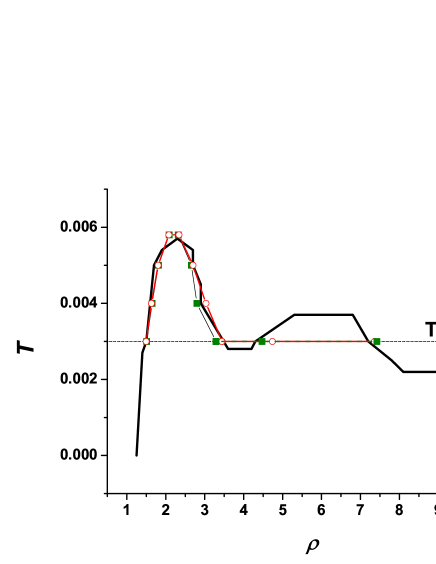
Figure 1: The phase diagram of a Hertz system with $\alpha$=7/2. The line shows the data from miller . The symbols show our results (see the text). The horizontal line marks the $T$=0.003 isotherm at which the study of the phase diagram at high density is performed in the present paper.

Another intriguing problem that is rarely discussed in literature is investigating heat capacity behavior in 2D melting. The peculiarities of heat capacity behavior in 2D melting can be related to a change in the density of topological defects. The BKT transition is an infinite order (continuous) phase transition. Continuous phase transitions are accompanied by divergences in thermodynamic quantities caused by the divergence of the correlation length as critical temperature $T_{c}$ is approached. For the BKT transition there is an exponential divergence of isochoric heat capacity $c_{v}(T)$ ch_l . It is so rapid and occurs within such a narrow temperature range that the divergence in $c_{V}$ cannot be resolved in simulations or in experiments ch_l . The value of $c_{v}$ measured for the BKT transition in an $X-Y$ model is sketched in Fig. 9.4.3 in Ref. ch_l and has unobservable essential singularity at $T_{c}$ and and a nonuniversal model-dependent maximum above $T_{c}$ associated with the entropy liberated by the unbinding of bound topological defect pairs. Using large-scale Monte Carlo simulation for the BKTHNY transition in a Lennard-Jones system wierschem the authors observed one broad peak in the specific heat per particle. In Ref. cv2d a melting transition of superparamagnetic colloidal spheres confined in two dimensions was studied. This system had long-range interaction and melted in accordance with the BKTHNY scenario, and it was shown that there was only one smooth peak inside the hexatic phase. At the same time in non-ideal Yukawa systems vaulina the BKTHNY transition is accompanied by two singularities (”jumps”) for the heat capacities near temperatures of the fluid-to-hexatic phase and hexatic-to-”perfect” (without defects) crystal transitions. The question is whether in the case of two-stage melting one would observe two peaks on the $c_{v}(T)$ curve and where these possible peaks would be located or there is only one peak related to the melting transition.

The goal of the present paper is to study the melting scenarios of a 2D Hertzian sphere system with control parameter $\alpha$=7/2 and to investigate the behavior of heat capacity $c_{v}(T)$ across the melting line.

II System and methods

The simulation setup is similar to the one described in Ref. molphys . We use rescaled number density $\tilde{\rho}=N\sigma^{2}/A$ and temperature $\tilde{T}=k_{B}T/\varepsilon$ and omit tildes in what follows. Firstly, we simulated a small system of 5000 particles in a rectangular box under periodic boundary conditions in a wide range of densities from $\rho_{min}$=0.5 to $\rho_{max}$=10.0 at temperature $T$=0.003. The molecular dynamics in a canonical ensemble (constant number of particles $N$, square of the system $A$, and temperature $T$) was used. According to Ref. miller , at this temperature there are two crystalline regions on this way: the first one in the range of densities (approximately) 1.5 - 3.5 and the second one in range 4.4 - 7.2. We roughly localize phase boundaries from the equations of state and radial distribution functions (rdfs) in a small system. The small systems are propagated for $5\cdot 10^{6}$ steps with time step $dt$=0.001. The first $2.5\cdot 10^{6}$ steps were used for equilibration and the last $2.5\cdot 10^{6}$ were used for production.

At the second step we used larger systems and smaller density intervals in order to locate precise phase boundaries. We used a system of 20000 particles at densities below 3.6 and 45000 particles above this threshold. The number of particles was increased at higher densities in order to evaluate the spatial correlation functions at large enough separations.

Special attention was paid to the region of the first maximum on the phase diagram. In this case we calculated a complete melting line up to a maximum. The simulation methodology was the same: we roughly localized phase boundaries simulating a small system and after that we performed simulations with 20000 particle systems to find precise phase boundaries.

In order to estimate the phase boundaries we used the method based on a combination of equations of state, orientational and translational order parameters and their correlation functions. The local orientational order parameter (OOP) was defined in the following way halpnel1 ; halpnel2 ; dfrt5 ; dfrt6 :

$$\psi_{6}({\bf r_{i}})=\frac{1}{n(i)}\sum_{j=1}^{n(i)}e^{in\theta_{ij}},$$ (2)

where $\theta_{ij}$ is the angle of the vector between particles $i$ and $j$ with respect to the reference axis and the sum over $j$ is counting the $n(i)$ nearest-neighbors of $j$, obtained from the Voronoi construction. The global OOP can be calculated as an average over all particles:

$$\Psi_{6}=\frac{1}{N}\left<\left|\sum_{i}\psi_{6}({\bf r}_{i})\right|\right>.$$ (3)

The translational order parameter (TOP) has the following form halpnel1 ; halpnel2 ; dfrt5 ; dfrt6 :

$$\Psi_{T}=\frac{1}{N}\left<\left|\sum_{i}e^{i{\bf Gr}_{i}}\right|\right>,$$ (4)

where ${\bf r}_{i}$ is the position vector of particle $i$ and G is the reciprocal-lattice vector of the first shell of the crystal lattice.

The orientational correlation function (OCF) is defined as

$$g_{6}(r)=\frac{\left<\Psi_{6}({\bf r})\Psi_{6}^{*}({\bf 0})\right>}{g(r)},$$ (5)

where $g(r)=<\delta({\bf r}_{i})\delta({\bf r}_{j})>$ is the pair distribution function. In the hexatic phase the long-range behavior of $g_{6}(r)$ has the form $g_{6}(r)\propto r^{-\eta_{6}}$ with $\eta_{6}\leq\frac{1}{4}$ halpnel1 ; halpnel2 .

Analogously, the translational correlation function (TCF) is given by

$$g_{T}(r)=\frac{<\exp(i{\bf G}({\bf r}_{i}-{\bf r}_{j}))>}{g(r)},$$ (6)

where $r=|{\bf r}_{i}-{\bf r}_{j}|$. In the solid phase the long-range behavior of $G_{T}(r)$ has the form $g_{T}(r)\propto r^{-\eta_{T}}$ with $\eta_{T}\leq\frac{1}{3}$ halpnel1 ; halpnel2 . In the hexatic phase and isotropic liquid $g_{T}$ decays exponentially.

In addition, we also studied the behavior of isochoric heat capacity along the phase transitions. The heat capacity was calculated from the fluctuation formula $c_{V}=\frac{<U^{2}>-<U>^{2}}{Nk_{B}(T)^{2}}$, where $U$ is the energy of the system book_fs . In the present paper we calculate the fluctuation of potential energy only, and therefore the values of the heat capacity are the difference between the full heat capacity and the ideal gas value $c_{V,id}=1$. For the sake of brevity we call it simply as $c_{V}$.

At the second stage of the work we performed longer simulations of $5\cdot 10^{7}$ steps. Moreover, $2D$ systems demonstrate extremely strong fluctuations, and the results were still noisy. In order to remove the noise we simulated several replicas of the system. The initial configuration was always a triangular crystal, but the initial velocities were different. Up to 80 replicas were used; however, in most cases 50 replicas gave acceptable accuracy. The final pressures and heat capacities were calculated by averaging over all replicas.

III Results and discussion

Firstly we studied the order parameters of a small system of 5000 particles (Fig. 2) at temperature $T$=0.003. We performed very quick calculations to roughly estimate phase boundaries. Fig. 2 shows the OOP and TOP of the system. One can see that there are two regions where both order parameters have finite values, i.e. the system has two zones where the crystalline phase is stable. These regions are $\rho=1.4\div 3.8$ and $\rho=4.4\div 7.8$. Therefore four regions of phase transitions can be identified. In Fig. 2 these regions are marked with letters from $a$ to $d$. Below we will use these letters to denote the regions of the phase diagram. In the vicinity of regions $a$ and $c$, an increase in density leads to the transformation of a liquid into solid, while at transition borders $b$ and $d$ re-entrant melting of the solid takes place. In order to obtain the phase boundaries more accurately, we studied these regions with a larger system and performed longer simulations (see the methods above).

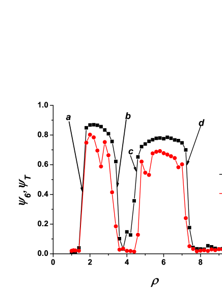
Figure 2: Orientational and translational order parameters $\psi_{6}$ and $\psi_{T}$ along isotherm $T$=0.003.

It is common knowledge that 2D systems demonstrate strong fluctuations. As a result one needs to collect a very large statistic in order to get reliable results. Although we performed rather long simulations ($5\cdot 10^{7}$ steps) we found that the accuracy of the results was not sufficient. Because of this we performed more simulations with different initial velocities. We called such configurations different replicas. Up to 80 replicas of the same system were considered. Fig. 3 (a) shows the equation of state of the system in region a for a different number of replicas. One can see that the results for a single replica are very noisy. In the case of 20 replicas the results are better, but still not very accurate. We find that only averaging over 80 replicas gives acceptable accuracy.

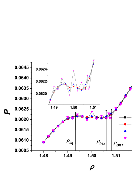
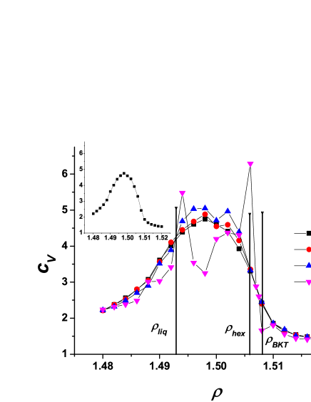
Figure 3: (a) Comparison of the equations of state for 80, 50, 20 and one replica of the system at $T$=0.003. The inset enlarges the region of the Mayer-Wood loop. (b) Comparison of heat capacity for 80, 50, 20 and one replica of the system at $T$=0.003. The inset shows the heat capacity for 80 replicas.

After averaging over 80 replicas we observed that the equation of state demonstrated the Mayer-Wood loop which signalizes the presence of a first-order phase transition (Fig. 3 (a)). In order to distinguish between the first and the third scenarios of melting we studied order parameters $\psi_{6}$ and $\psi_{T}$ and their correlation functions in a system of 20000 particles. Fig. 4 shows the translational and orientational correlation functions of the system in the region of melting at the lowest densities. One can see that the transition from the crystal into hexatic phase occurs at density $\rho_{BKT}$=1.508. The instability of the hexatic phase takes place at $\rho$=1.496, which is in the middle of the Mayer-Wood loop. This situation corresponds to the third melting scenario, i.e. the continuous BKT transition from the solid to hexatic phase and the first-order one from the hexatic phase to the isotropic liquid. The densities of the hexatic and liquid phases at coexistence are $\rho_{hex}$=1.506 and $\rho_{liq}$=1.493.

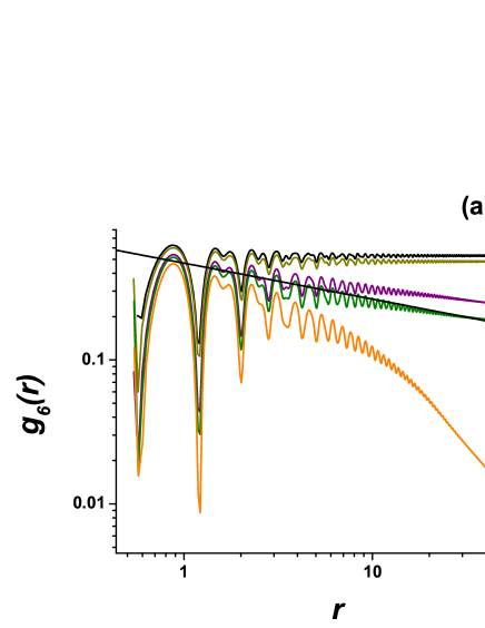
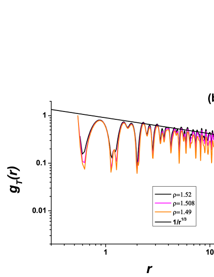
Figure 4: (a) The translational and (b) orientational correlation functions of the system in the density region corresponding to a transition from liquid into a triangular phase at low density (region a in terms of Fig. 2 (b)). $T$=0.003.

We also studied the isochoric heat capacity of the system (Fig. 3 (b)). One can see that the heat capacity is more sensitive to the quality of statistical averaging than the equation of state. It demonstrates a single peak at $\rho$=1.498 after averaging over 80 replicas. Besides, $c_{V}$ demonstrates a small second peak at $\rho$=1.502 with 50 replicas. One can conclude that inappropriate averaging can lead to qualitatively wrong results in the case of 2D systems. The real peak appears inside the Mayer-Wood loop of the hexatic to liquid transition, in the neighborhood of the hexatic phase stability limit. As discussed in the Introduction, one can conclude from Fig. 3 (b) that the peak is related to a solid-hexatic transition. In this case the BKT transition occurs at $\rho_{BKT}$=1.508 with unobservable essential singularity at $\rho_{BKT}$ and a nonuniversal model-dependent ”bump” below $\rho_{BKT}$ associated with the entropy liberated by the unbinding of dislocation pairs. It is interesting to note, that due to this very thorough averaging we do not observe a possible $\delta$ function peak related to a first-order hexatic-liquid transition.

We proceeded by a more detailed investigation of region $b$ (see Fig. 2). Here the equation of state and heat capacity are less noisy and 50 replicas of the system are sufficient to get reasonable statistical averaging. Figs. 5 (a) and (b) show the equation of state and the heat capacity of the system in region $b$ at temperature $T$=0.003. One can see that the equation of state does not demonstrate any loops, therefore we do not observe a first order phase transition. The system melts in accordance with the BKTHNY scenario. Figs. 6 shows the OCF (panel a) and TCF (panel b) of the system in region $b$. One can see that the crystal to hexatic transition takes place at $\rho_{sh}$=3.28 and from the hexatic to liquid phase at $\rho_{hl}$=3.45. It is also shown that the maximum of heat capacity is located in the neighborhood of the hexatic phase stability limit and near the hexatic to liquid transition.

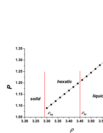
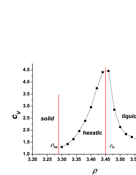
Figure 5: (a) The equation of state and (b) heat capacity of the system in region $b$. $T$=0.003.

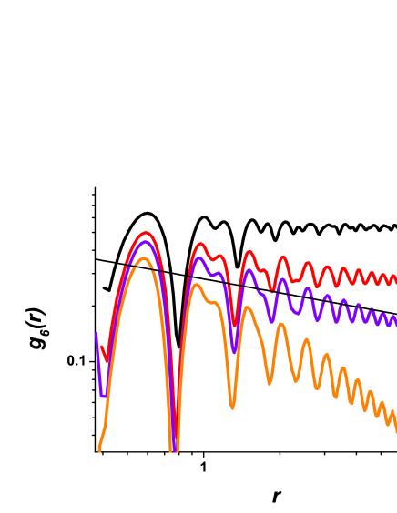
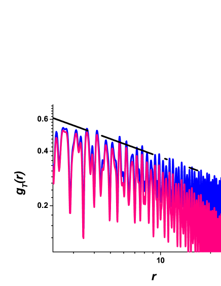
Figure 6: (a) The orientational and (b) translational correlation functions in region $b$. $T$=0.003.

Let us consider the melting line in regions $a$ and $b$ at higher temperatures. Fig. 7 shows the equations of state in region $a$ at three different temperatures. One can see the Mayer-Wood loop $T$=0.004. However, at $T$=0.005 the Mayer-Wood loop disappears. Therefore, the melting scenarios change and melting proceeds in accordance with the BKTHNY theory. No loop is observed at $T$=0.0058.

A system of Hertz spheres with $\alpha$=5/2 was studied in our previous work molphys . It was shown that the melting line of the low density triangular crystal had two tricritical points: at the maximum on the melting line and at $T$=0.0034 at the right branch (region $b$ in the notation of the present paper). The results of this paper demonstrate that Hertz spheres with $\alpha$=7/2 have only one tricritical point at the left branch (region $a$). No changes of the melting scenarios take place at the maximum of the melting line.

Figure 7: The isotherms of the system crossing the melting line in region $a$.

The melting line of a low density triangular crystal is shown in Fig. 8. The location of heat capacity maxima is also shown. One can see that the heat capacity maximum almost coincides with the disappearance of orientational order in accordance with the OCF. In the case of a single first order hexatic to liquid transition it is located in a two-phase region (see, for example, Fig. 3 (b)). In the case of the BKTHNY scenario a heat capacity maximum is located near the hexatic to isotropic liquid transition (Fig. 5). But in both cases the heat capacity maximum is close to the hexatic phase stability limit. It is interesting, that the heat capacity demonstrates peaks even at $T$=0.0025 and $\rho$=3.9. This temperature is below the minimum of the melting line and is deep inside the solid phase. The location of the heat capacity peak seems to coincide with the density of the minimum of the melting line. Also the height of the maximum is much lower compared with the peaks related to the melting transition. One can suppose that in the vicinity of the melting line minimum there is smooth structural reconstruction producing this maximum.

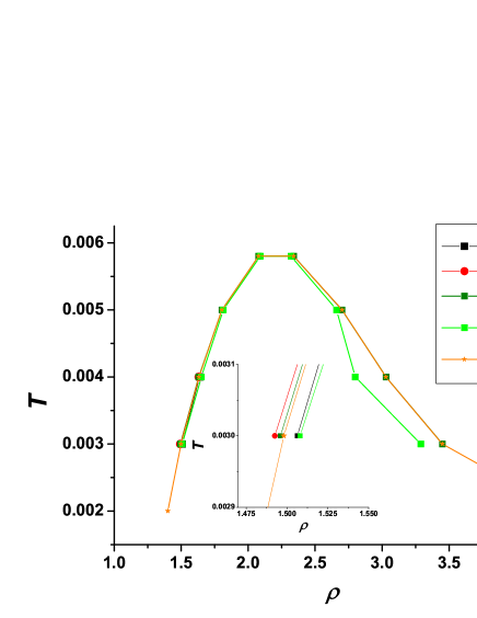
Figure 8: The melting line of a low density triangular crystal (regions $a$ and $b$). The inset enlarges region a at $T$=0.003. The location of the heat capacity maxima is also shown. The loop - is the points obtained from the Mayer-Wood loop, $g_{6}$ - is a solid to hexatic transition from the OCF, $g_{T}$ - is a hexatic to isotropic liquid transition from the TCF, $c_{V}max$ - is the location of the heat capacity maxima.

We proceed with considering region $c$. Here we again performed simulation of 50 replicas in order to get a reliable statistic. The equation of state again does not demonstrate the Mayer-Wood loop (Fig. 9 (a)), therefore the BKTHNY scenario is realized in this case. The maximum of heat capacity appears at $\rho$=4.48 (Fig. 9 (b)).

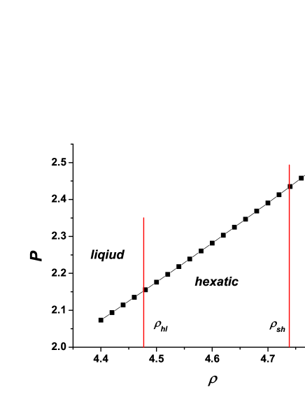
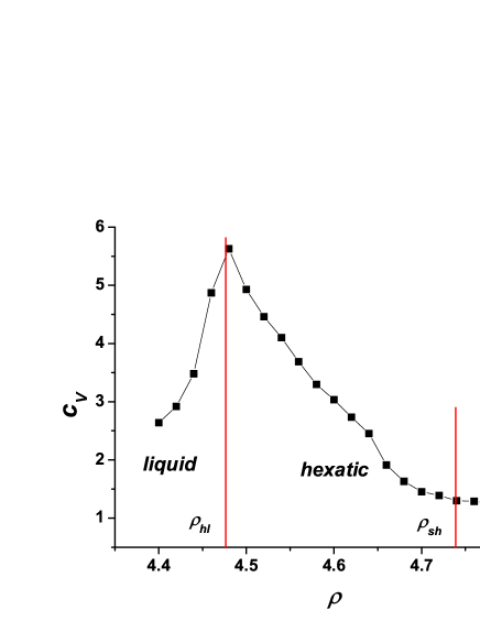
Figure 9: (a) The equation of state and (b) heat capacity of the system in region $c$ at $T$=0.003.

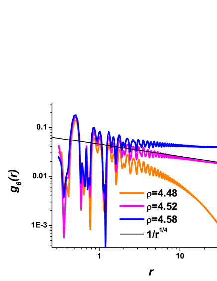
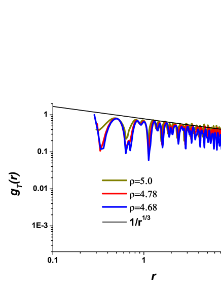
Figure 10: ((a) The orientational and (b) translational correlation functions in region $c$ at $T$=0.003.

The limits of stability of the solid and hexatic phases are obtained from correlation functions $g_{6}$ and $g_{T}$ (Fig. 10). The solid to hexatic transition takes place at density $\rho_{sh}$=4.74 and the hexatic to liquid one at $\rho_{hl}$=4.472. It means that the peak of heat capacity appears close to the hexatic to liquid transition.

Finally we studied the system in region $d$. The equation of state at $T$=0.003 does not demonstrate the Meyer-Wood loop, and one can conclude that in this region the system melts in accordance with the BKTHNY scenario. The situation is similar to regions $b$ and $c$. From the long-range behavior of the OCF and TCF one can see that the transition from solid to hexatic phase takes place at $\rho_{sh}$=7.36 and the transformation of the hexatic phase into the isotropic liquid occurs at $\rho_{hl}$=7.42.

In Ref. miller it was found that the melting line of a Hertzian system with $\alpha$=7/2 had a complex shape with multiple maxima and minima. Our calculations confirm this unusual result. However, the nature of such a complex shape of the melting line of the same phase remains vague. To shed light on this problem we studied the equations of state and the structure of the solid phase in the region of densities from b to c below the melting line.

Fig. 11 (a) shows the first peak of the rdf at $T$=0.002 as a function of density. Usually with an increase in density the location of the first peak shifts towards smaller $r$’s while its height increases. Here we clearly see that although the location of the first peak behaves normally (Fig. 11 (b)) its height decreases with density increasing to $\rho$=4.0 where a minimum is observed (Fig. 11 (c)). This density of the minimum is close to the density of the melting line minimum. Such unusual behavior of the rdfs is well known in liquids where it signalizes smooth structural crossover, i.e. the structure changes without a phase transition. A structural crossover in liquids usually leads to the appearance of a maximum on the melting line (see, for example, book1 ). In the present work the situation is more complex: there is no change in the structure (only a triangular crystal is observed), however, the unusual dependence of its rdfs leads to the appearance of a minimum on the melting line.

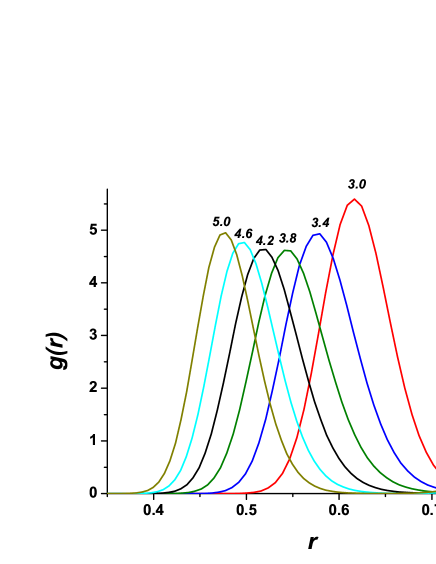
Figure 11: (a) The first peak of the rdf at $T$=0.002. (b) The location of the first peak of the rdf at $T$=0.002. (c) The height of the first peak of the rdf at $T$=0.002.

Another unusual property of the phase diagram is its quasi-periodic shape. In the density interval up to $rho$=10.0 which was studied in miller there are three peaks. Such complex phase diagrams can be observed in core-softened systems with several length scales in the potential dfrt1 ; dfrt2 ; dfrt3 ; dfrt5 ; we5 . In the case of deformable Hertzian potential there is only one length scale. Here we suppose, that complex phase behavior can be related to the absence of singularity of the potential in the origin and to high compressibility of the system. As a result of these two factors, more coordination spheres come into the realm of potential influence when the system is compressed. Fig. 12 shows the rdfs of the system in the vicinity of the phase transition regions. Regions $a$ and $c$ correspond to normal melting, i.e. the melting curve has a positive slope in these regions (a solid is denser than a liquid), while regions $b$ and $d$ are re-entrant melting regions, i.e. the liquid has higher density than the solid. The vertical line shows the potential cut-off distance. One can see that in region $a$ the first peak of the rdf is within the potential range while the first minimum is out of it. In the vicinity of region $b$ the first minimum of the rdf is within the potential cut-off distance, while the second maximum is still out of potential cut-off. The system crystallizes again in region $c$ where the second peak is within the interaction range. Finally, in region $d$ the second minimum is inside the potential cut-off distance. From these observations we see that when a peak of the rdf occurs in the distance within the interaction range ($r$=1.0) the system crystallizes, while when a minimum of the rdf takes place in this realm the system experiences re-entrant melting. Therefore, crystallization of the system is strongly influenced by the number of coordination shells within the interaction range.

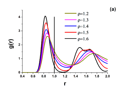
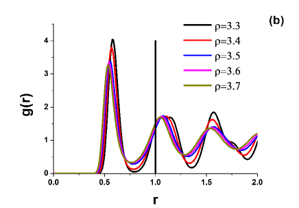
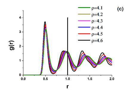
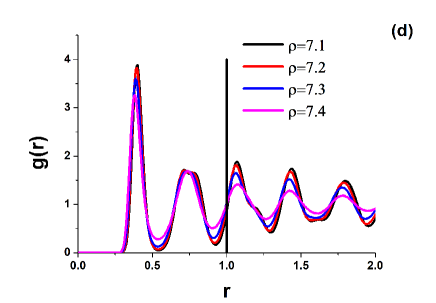
Figure 12: The radial distribution functions along the $T$=0.003 isotherms in the vicinity of the regions of phase transitions. Panels a, b, c and d correspond to regions $a$, $b$, $c$, and $d$. The vertical line shows the $r$=1.0 threshold, which is the realm of influence of the potential.

In order to evaluate the influence of different coordination shells we performed the following procedure. In the case of an ideal triangular lattice the relation between the density and the lattice parameter is $a=\rho\sqrt{3}/2$. The second neighbor distance is $a\sqrt{3}$ and the third one is $2a$. The particles interact if the distance between them is below cut off $r_{c}$=1.0. Therefore, we can calculate how many coordination shells are within the interaction range for some density of a triangular lattice.

At $T$=0 the particles start to interact (i.e. the distance between the nearest neighbors becomes equal to unity) at density $\rho$=1.1547 (the Start point in Fig. 13). This point corresponds to crystallization at branch $a$ of the melting line. The contribution of the first neighbors to the energy becomes positive $U_{1}\neq 0$, while the contribution of the highest order neighbors is zero $U_{2}=U_{3}=U_{4}$=0. The $Max-1$ point corresponds to the first maximum of the melting line (the merging of the $a$ and $b$ regions). At this point the energy is still determined by the first coordination shell only. The $Min-1$ point is at $\rho$=3.9 where the minimum of the melting line takes place. At this point the second coordination shell comes into the interaction distance. The second maximum of the melting line is denoted as $Max-2$. At this point three coordination shells are within the interaction range. Finally, at the second minimum of the melting line (point $Min-2$) four coordination shells are within the cut-off distance. One can see that when an odd number of coordination shells is within the cut-off distance the melting line has a positive slope and the solid density is higher than the density of the corresponding liquid, whilst when the number of coordination shells becomes even the melting curve passes the maximum and turns to a negative slope with the liquid density higher than the solid one. Therefore, the complex shape of the phase diagram should be related to the inclusion of higher order neighbors in the interaction range.

IV Conclusions

The paper presents a molecular dynamics simulation study of the phase diagram and melting scenarios of a two-dimensional system of Hertzian spheres with control parameter $\alpha$=7/2 previously studied in Ref. miller . It is shown that depending on the position on the phase diagram, the system can melt both in accordance with the Berezinskii-Kosterlitz-Thouless-Halperin-Nelson-Young (BKTHNY) scenario (two continuous transitions with an intermediate hexatic phase) as well as through a two-stage melting with a first-order hexatic-isotropic liquid transition and a continuous solid-hexatic BKT transition. The behavior of heat capacity was studied. We show that despite two-stage melting, the heat capacity has one peak which seems to correspond to a solid-hexatic transition. This peak is a nonuniversal model-dependent maximum below the solid-hexatic transition density associated with the entropy liberated by the unbinding of bound dislocation pairs str ; ch_l . In the case of the first-order hexatic-liquid transition the heat capacity peak is located inside the two-phase region while in the case of the BKTHNY scenario the peak is inside the hexatic phase in the vicinity of the hexatic-liquid transition. The form of the phase diagram is related to the number of coordination shells inside the potential range.

Figure 13: The interaction potential of a Hertzian system with $\alpha$ =7/2 with special points (see the text).

V Acknowledgments

We are grateful to V.V. Brazhkin, and E.E. Tareyeva for stimulating discussions. This work was carried out using computing resources of the federal collective usage centre ”Complex for simulation and data processing for mega-science facilities” at NRC ”Kurchatov Institute”, http://ckp.nrcki.ru, and supercomputers at Joint Supercomputer Center of the Russian Academy of Sciences (JSCC RAS). The work was supported by the Russian Foundation for Basic Research (Grants No 17-02-00320 (VNR) and 18-02-00981 (YDF))

References

- (1) C. N. Likos, Soft Matter, 2006, 2, 478.
- (2) A. Fernandez-Nieves and A. M. Puertas, Fluids, colloids, and soft materials: an introduction to soft matter physics, Wiley, 2016.
- (3) A. Ivlev, H. Lowen, G. Morfill and C. P. Royall, Complex plasmas and Colloidal dispersions: particle-resolved studies of classical liquids and solids (Series in soft condensed matter), Word Scientific, Singapore, 2012.
- (4) C. N. Likos, A. Lang, M. Watzlawek, and H. Lowen, Phys. Rev. E: Stat. Phys., Plasmas, Fluids, Relat. Interdiscip. Top., 2001, 63, 031206.
- (5) L. Athanasopoulou and P. Ziherl, Soft Matter, 2017, 13, 1463.
- (6) Bo Li, Xiuming Xiao, Shuxia Wang, Weijia Wen, and Ziren Wang, Phys. Rev. X, 2019, 9, 031032.
- (7) B. van der Meer, L. Filion and M. Dijkstra, Soft Matter,2016, 12, 3406 3411.
- (8) N. Elsner, C. P. Royall, B. Vincent and D. R. E. Snoswell, J. Chem. Phys., 2009, 130, 154901.
- (9) Z. V. Vardeny, A. Nahata and A. Agrawal, Nat. Photonics, 2013, 7, 177 187.
- (10) K. I. Zaytsev and S. O. Yurchenko, Appl. Phys. Lett., 2014, 105, 051902.
- (11) K. I. Zaytsev, G. M. Katyba, E. V. Yakovlev, V. S. Gorelik and S. O. Yurchenko, J. Appl. Phys., 2014, 115, 213505.
- (12) S. O. Yurchenko, K. I. Zaytsev, E. A. Gorbunov, E. V. Yakovlev, A. K. Zotov, V. M. Masalov, G. A. Emelchenko and V. S. Gorelik, J. Phys. D: Appl. Phys., 2017, 50, 055105.
- (13) K. Edagawa, Sci. Technol. Adv. Mater., 2014, 15, 034805.
- (14) S. Prestipino, F. Saija and G. Malescio, Soft Matter, 2009, 5, 2795.
- (15) A. Suto, Phys. Rev. B: Condens. Matter Mater. Phys., 2006, 74, 104117.
- (16) C. N. Likos, Nature, 2006, 440, 433.
- (17) J. Pamies, A. Cacciuto and D. Frenkel, J. Chem. Phys., 2009, 131, 044514.
- (18) S. A. Rice, Chem. Phys. Lett., 2009, 479, 1.
- (19) D. E. Dudalov, Yu. D. Fomin, E. N. Tsiok, and V. N. Ryzhov, J. Phys.: Conference Series, 2014, 510, 012016.
- (20) D. E. Dudalov, Yu. D. Fomin, E. N. Tsiok, and V. N. Ryzhov, J. Chem. Phys., 2014, 141, 18C522.
- (21) D. E. Dudalov, Yu. D. Fomin, E. N. Tsiok, and V. N. Ryzhov, Soft Matter, 10, 4966.
- (22) E. N. Tsiok, D. E. Dudalov, Yu. D. Fomin, and V. N. Ryzhov, Phys. Rev. E: Stat. Phys., Plasmas, Fluids, Relat. Interdiscip. Top., 2015, 92, 032110.
- (23) N. P. Kryuchkov, S. O. Yurchenko, Yu. D. Fomin, E. N. Tsiok, and V. N. Ryzhov, Soft Matter, 2018, 14, 2152.
- (24) Zach Krebs, Ari B. Roitman, Linsey M. Nowack, Chris Liepold, Binhua Lin, and Stuart A. Rice, J. Chem. Phys., 2018, 149, 034503.
- (25) J. C. Pamies, A. Cacciuto, and D. Frenkel, J. Chem. Phys., 2009, 131, 044514.
- (26) Yu. D. Fomin, V. N. Ryzhov, N. V. Gribova, Phys. Rev. E: Stat. Phys., Plasmas, Fluids, Relat. Interdiscip. Top., 2010, 81, 061201.
- (27) Yu. D. Fomin, E. A. Gaiduk, E. N. Tsiok, and V. N. Ryzhov, Molecular Physics, 2018, 116, 3258-3270.
- (28) W. L. Miller, A. Cacciuto, Soft Matter, 2011, 7, 7552.
- (29) M. Zum J. Liu, H. Tong and N. Xu, Phys. Rev. Lett., 2016, 117, 085702.
- (30) M. Zu, P. Tan and N. Xu, Nature Comm., 2017, 8, 2089.
- (31) V. N. Ryzhov, E. E. Tareyeva, Yu. D. Fomin, E. N. Tsiok, Phys.-Usp., 2017, 60, 857.
- (32) S. T. Chui, Phys. Rev. B: Condens. Matter Mater. Phys., 1983, 28, 178.
- (33) V. N. Ryzhov, Sov. Phys. JETP, 1991, 73, 899.
- (34) V. N. Ryzhov and E. E. Tareyeva, Physica A, 2002, 314, 396.
- (35) V. N. Ryzhov and E. E. Tareyeva, Phys. Rev. B: Condens. Matter Mater. Phys., 1995, 51 8789.
- (36) V. N. Ryzhov and E. E. Tareeva, Sov. Phys. JETP, 1995, 81, 1115.
- (37) V. L. Berezinskii, Sov. Phys. JETP, 1971, 32, 493.
- (38) V. L. Berezinskii, Sov. Phys. JETP, 1972, 34, 610.
- (39) J. M. Kosterlitz and D. J. Thouless, J. Phys. C: Solid State Phys., 1972, 5, L124.
- (40) J. M. Kosterlitz and D.J. Thouless, J. Phys. C: Solid State Phys., 1973, 6, 1181.
- (41) J. M. Kosterlitz, Rep. Prog. Phys., 2016, 79, 026001.
- (42) B. I. Halperin and D. R. Nelson, Phys. Rev. Lett., 1978, 41, 121.
- (43) D. R.Nelson and B. I. Halperin, Phys. Rev. B: Condens. Matter Mater. Phys., 1979, 19, 2457.
- (44) A. P. Young, Phys. Rev. B: Condens. Matter Mater. Phys., 1979, 19, 1855.
- (45) K. J. Strandburg, Rev. Mod. Phys., 1988, 60, 161.
- (46) Urs Gasser, C. Eisenmann, G. Maret, and P. Keim, Phys. Chem. Chem. Phys., 2010, 11, 963.
- (47) K. Zahn and G. Maret, Phys. Rev. Lett., 2000, 85, 3656.
- (48) P. Keim, G. Maret, and H.H. von Grunberg, Phys. Rev. E: Stat. Phys., Plasmas, Fluids, Relat. Interdiscip. Top., 2007, 75, 031402.
- (49) S. Deutschlander, T. Horn, H. Lowen, G. Maret, and P. Keim, Phys. Rev. Lett., 2013, 111, 098301.
- (50) T. Horn, S. Deutschlander, H. Lowen, G. Maret, and P. Keim, Phys. Rev. E: Stat. Phys., Plasmas, Fluids, Relat. Interdiscip. Top., 2013, 88, 062305.
- (51) E. P. Bernard and W. Krauth, Phys. Rev. Lett., 2011, 107, 155704.
- (52) M. Engel, J. A. Anderson, S. C. Glotzer, M. Isobe, E. P. Bernard, W. Krauth, Phys. Rev. E: Stat. Phys., Plasmas, Fluids, Relat. Interdiscip. Top., 2013, 87, 042134.
- (53) W. Qi, A. P. Gantapara and M. Dijkstra, Soft Matter, 2014, 10, 5449.
- (54) S.C. Kapfer and W. Krauth, Phys. Rev. Lett., 2015, 114, 035702.
- (55) W. Qi and M. Dijkstra, Soft Matter, 2015, 11, 2852.
- (56) A. L. Thorneywork, J. L. Abbott, D. G. A. L. Aarts, and R. P. A. Dullens, Phys. Rev. Lett., 2017, 118, 158001.
- (57) E. A. Gaiduk, Yu.D. Fomin, E. N. Tsiok and V. N. Ryzhov, Molecular Physics 2019, 117, 2910.
- (58) E. N. Tsiok, Y. D. Fomin, V. N. Ryzhov, Physica A, 2018, 490, 819.
- (59) G. Algara-Siller, O. Lehtinen, F. C. Wang, R. R. Nair, U. Kaiser, H. A. Wu, A. K. Geim and I. V. Grigorieva, Nature, 2015, 519, 443.
- (60) J. Zhao, Q. Deng, A. Bachmatiuk, G. Sandeep, A. Popov, J. Eckert, M. H. Rummeli, Science, 2014, 343, 1228.
- (61) N. Osterman, D. , I. Poberaj, J. Dobnikar, and P. Ziherl, Phys. Rev. Lett., 2007, 99, 248301.
- (62) A. Jain, J. R. Errington and Th. M. Truskett, Phys. Rev. X, 2014, 4, 031049.
- (63) E. Marcotte, F. H. Stillinger, and S. Torquato, J. Chem. Phys., 2011, 134, 164105.
- (64) W. D. Pineros, M. Baldea, and Th. M. Truskett, J. Chem. Phys., 2016, 145, 054901.
- (65) M. Engel and H. R. Trebin, Phys. Rev. Lett., 2007, 98, 225505.
- (66) T. Dotera, T. Oshiro, and P. Ziherl, Nature, 2014, 506, 208 211.
- (67) H. Pattabhiraman and M. Dijkstra, J. Chem. Phys., 2017, 146, 114901.
- (68) S. Deutschländer, A. M. Puertas, G. Maret, and P. Keim, Phys. Rev. Lett., 2014, 113, 127801.
- (69) P. M. Chaikin and T. C. Lubensky, Principles of condensed matter physics, Cambridge University Press, 1995.
- (70) K. Wierschem and E. Manousakis, Phys. Rev. B: Condens. Matter Mater. Phys., 2011, 83, 214108.
- (71) O. S. Vaulina, X. G. Koss (Adamovich), Physics Letters A, 2009, 373, 3330.
- (72) http://lammps.sandia.gov/
- (73) D. Frenkel and B. Smit, Understanding molecular simulation (From Algorithms to Applications), 2nd Edition, Academic Press, 2002.
- (74) V. V. Brazhkin. S. V. Buldyrev, V. N. Ryzhov, and H. E. Stanley [eds], New Kinds of Phase Transitions: Transformations in Disordered Substances, Proc. NATO Advanced Research Workshop, Volga River, Kluwer, Dordrecht, 2002.