Supplementary material for Uncorrected least-squares temporal difference with lambda-return

Abstract

Here, we provide a supplementary material for Takayuki Osogami, “Uncorrected least-squares temporal difference with lambda-return,” which appears in Proceedings of the 34th AAAI Conference on Artificial Intelligence (AAAI-20) (Osogami, 2019).

Appendix A Proofs

In this section, we prove Theorem 1, Lemma 1, Theorem 2, Lemma 2, and Proposition 1. Note that equations (1)-(19) refers to those in Osogami (2019).

A.1 Proof of Theorem 1

From (7)-(8), we have the following equality:

$${\mathbf{A}}^{\rm Unc}_{T+1} =\sum_{t=0}^{T}{\boldsymbol{\phi}}_{t}\left({\boldsymbol{\phi}}_{t}-(1-\lambda)\,\gamma\sum_{m=1}^{T-t}(\lambda\,\gamma)^{m-1}\,{\boldsymbol{\phi}}_{t+m}\right)^{\top}$$ (20)

$$=\sum_{t=0}^{T-1}{\boldsymbol{\phi}}_{t}\left({\boldsymbol{\phi}}_{t}-(1-\lambda)\,\gamma\sum_{m=1}^{T-t}(\lambda\,\gamma)^{m-1}\,{\boldsymbol{\phi}}_{t+m}\right)^{\top}+{\boldsymbol{\phi}}_{T}\,{\boldsymbol{\phi}}_{T}^{\top}$$ (21)

$$=\sum_{t=0}^{T-1}{\boldsymbol{\phi}}_{t}\Bigg{(}{\boldsymbol{\phi}}_{t}-(1-\lambda)\,\gamma\sum_{m=1}^{T-t-1}(\lambda\,\gamma)^{m-1}\,{\boldsymbol{\phi}}_{t+m}-(1-\lambda)\,\gamma(\lambda\,\gamma)^{T-t-1}\,{\boldsymbol{\phi}}_{T}\Bigg{)}^{\top}+{\boldsymbol{\phi}}_{T}\,{\boldsymbol{\phi}}_{T}^{\top}$$ (22)

$$={\mathbf{A}}^{\rm Unc}_{T}-\sum_{t=0}^{T-1}{\boldsymbol{\phi}}_{t}(1-\lambda)\,\gamma\,(\lambda\,\gamma)^{T-t-1}\,{\boldsymbol{\phi}}_{T}^{\top}+{\boldsymbol{\phi}}_{T}\,{\boldsymbol{\phi}}_{T}^{\top}$$ (23)

$$={\mathbf{A}}^{\rm Unc}_{T}+\left(\sum_{t=0}^{T}(\lambda\,\gamma)^{T-t}\,{\boldsymbol{\phi}}_{t}\right){\boldsymbol{\phi}}_{T}^{\top}-\gamma\left(\sum_{t=0}^{T-1}(\lambda\,\gamma)^{T-t-1}\,{\boldsymbol{\phi}}_{t}\right){\boldsymbol{\phi}}_{T}^{\top}$$ (24)

$$={\mathbf{A}}^{\rm Unc}_{T}+({\mathbf{z}}_{T}-\gamma\,{\mathbf{z}}_{T-1})\,{\boldsymbol{\phi}}_{T}^{\top}.$$ (25)

$${\mathbf{b}}_{T+1} =\sum_{t=0}^{T}{\boldsymbol{\phi}}_{t}\sum_{m=0}^{T-t}(\lambda\,\gamma)^{m}\,r_{t+1+m}$$ (26)

$$=\sum_{t=0}^{T-1}{\boldsymbol{\phi}}_{t}\left(\sum_{m=0}^{T-t-1}(\lambda\,\gamma)^{m}\,r_{t+1+m}+(\lambda\,\gamma)^{T-t}\,r_{T+1}\right)+{\boldsymbol{\phi}}_{T}\,r_{T+1}$$ (27)

$$={\mathbf{b}}_{T}+{\mathbf{z}}_{T}\,r_{T+1}.$$ (28)

Here, the equality from (24) to (25) and the equality from (27) to (28) follow from the definition of the eligibility trace ${\mathbf{z}}_{T}$ in the theorem. The recursive computation of the eligibility trace can be verified in a straightforward manner. This completes the proof of Theorem 1.

A.2 Proof of Lemma 1

Observe that there exists $T_{0}$ such that $\frac{1}{T}{\mathbf{A}}_{T}^{\rm Unc}$ is invertible for any $T>T_{0}$, because we assume that $\frac{1}{T}{\mathbf{A}}_{T}^{\rm Unc}$ converges to an invertible matrix as $T\to\infty$, and invertible matrices form an open set. Then for each $T>T_{0}$, we have

$$\frac{1}{T}{\mathbf{A}}_{T}^{\rm Unc}\,({\boldsymbol{\theta}}_{T}-{\boldsymbol{\theta}}_{T}^{\star}) =\frac{1}{T}({\mathbf{b}}_{T}-{\mathbf{b}}_{T}^{\star})$$ (29)

$$({\boldsymbol{\theta}}_{T}-{\boldsymbol{\theta}}_{T}^{\star}) =\left(\frac{1}{T}{\mathbf{A}}_{T}^{\rm Unc}\right)^{-1}\,\frac{1}{T}({\mathbf{b}}_{T}-{\mathbf{b}}_{T}^{\star}).$$ (30)

By the continuity of matrix inverse, we then have

$$\lim_{T\to\infty}({\boldsymbol{\theta}}_{T}-{\boldsymbol{\theta}}_{T}^{\star}) =\left(\lim_{T\to\infty}\frac{1}{T}{\mathbf{A}}_{T}^{\rm Unc}\right)^{-1}\lim_{T\to\infty}\frac{1}{T}({\mathbf{b}}_{T}-{\mathbf{b}}_{T}^{\star}).$$ (31)

It thus suffices to show $\frac{1}{T}|{\mathbf{b}}_{T}^{\star}-{\mathbf{b}}_{T}|\to 0$ as $T\to\infty$.

Because the state space ${\cal S}$ is finite, the magnitude of the immediate reward and the feature vector is uniformly bounded. Namely, there exists $c<\infty$ such that $R(s)\leq c$ and $|{\boldsymbol{\phi}}(s)|\leq c$ elementwise for any $s\in{\cal S}$. Thus, we have the following elementwise inequality:

$$\frac{1}{T}|{\mathbf{b}}_{T}^{\star}-{\mathbf{b}}_{T}| =\frac{1}{T}\left|\sum_{t=0}^{T-1}{\boldsymbol{\phi}}_{t}\,\lambda^{T-t-1}\sum_{m=T-t}^{\infty}\gamma^{m}\sum_{s^{\prime}\in{\cal S}}({\mathbf{P}}^{m})_{s,s^{\prime}}\,R(s^{\prime})\right|$$ (32)

$$\leq c^{2}\,\frac{1}{T}\sum_{t=0}^{T-1}\lambda^{T-t-1}\sum_{m=T-t}^{\infty}\gamma^{m}\sum_{s^{\prime}\in{\cal S}}({\mathbf{P}}^{m})_{s,s^{\prime}}$$ (33)

$$=c^{2}\,\frac{1}{T}\sum_{t=0}^{T-1}\lambda^{T-t-1}\sum_{m=T-t}^{\infty}\gamma^{m}$$ (34)

$$=c^{2}\,\frac{1}{T}\sum_{t=0}^{T-1}\lambda^{T-t-1}\,\frac{\gamma^{T-t}}{1-\gamma}$$ (35)

$$=c^{2}\,\frac{\gamma}{1-\gamma}\,\frac{1}{T}\sum_{t=0}^{T-1}(\lambda\,\gamma)^{T-t-1}$$ (36)

$$=c^{2}\,\frac{\gamma}{1-\gamma}\,\frac{1}{T}\,\frac{1-(\lambda\,\gamma)^{T}}{1-\lambda\,\gamma},$$ (37)

which tends to 0 as $T\to\infty$. This completes the proof of Lemma 1.

A.3 Proof of Theorem 2

At each step $T$, Uncorrected LSTD($\lambda$) gives the weights ${\boldsymbol{\theta}}_{T}$, which is the solution of $\frac{1}{T}{\mathbf{A}}_{T}^{\rm Unc}\,{\boldsymbol{\theta}}=\frac{1}{T}{\mathbf{b}}_{T}$. Therefore, it suffices to show $\frac{1}{T}{\mathbf{A}}_{T}^{\rm Unc}\to\bar{\mathbf{A}}$ and $\frac{1}{T}{\mathbf{b}}_{T}\to\bar{\mathbf{b}}$ as $T\to 0$.

Due to the ergodicity of the Markov chain, as $T\to\infty$, each state is visited infinitely often, and the time each state is occupied is proportional to the steady state probability almost surely. Then, by the pointwise ergodic theorem, we have the following almost sure convergence:

$$\lim_{T\to\infty}\frac{1}{T}{\mathbf{A}}^{\rm Unc}_{T} =\lim_{T\to\infty}\frac{1}{T}\sum_{t=0}^{T-1}{\boldsymbol{\phi}}_{t}\left({\boldsymbol{\phi}}_{t}-(1-\lambda)\,\gamma\sum_{m=1}^{T-t-1}(\lambda\,\gamma)^{m-1}\,{\boldsymbol{\phi}}_{t+m}\right)^{\top}$$ (38)

$$=\sum_{s\in{\cal S}}{\boldsymbol{\pi}}(s)\,{\boldsymbol{\phi}}(s)\Bigg{(}\sum_{m=0}^{\infty}(\lambda\,\gamma)^{m}\sum_{s^{\prime}\in{\cal S}}({\mathbf{P}}^{m})_{s,s^{\prime}}\,{\boldsymbol{\phi}}(s^{\prime})-\gamma\sum_{m=1}^{\infty}(\lambda\,\gamma)^{m-1}\sum_{s^{\prime}\in{\cal S}}({\mathbf{P}}^{m})_{s,s^{\prime}}\,{\boldsymbol{\phi}}(s^{\prime})\Bigg{)}^{\top}$$ (39)

$$={\boldsymbol{\Phi}}^{\top}{\rm Diag}({\boldsymbol{\pi}})\,({\mathbf{I}}-\lambda\,\gamma\,{\mathbf{P}})^{-1}\,{\boldsymbol{\Phi}}-\gamma\,{\boldsymbol{\Phi}}^{\top}{\rm Diag}({\boldsymbol{\pi}})\,{\mathbf{P}}\,({\mathbf{I}}-\lambda\,\gamma\,{\mathbf{P}})^{-1}\,{\boldsymbol{\Phi}}$$ (40)

$$={\boldsymbol{\Phi}}^{\top}{\rm Diag}({\boldsymbol{\pi}})\,({\mathbf{I}}-\gamma\,{\mathbf{P}})\,({\mathbf{I}}-\lambda\,\gamma\,{\mathbf{P}})^{-1}\,{\boldsymbol{\Phi}}$$ (41)

and

$$\lim_{T\to\infty}\frac{1}{T}{\mathbf{b}}_{T} =\lim_{T\to\infty}\frac{1}{T}\sum_{t=0}^{T-1}{\boldsymbol{\phi}}_{t}\sum_{m=0}^{T-t-1}(\lambda\,\gamma)^{m}\,r_{t+1+m}$$ (42)

$$=\sum_{s\in{\cal S}}{\boldsymbol{\pi}}(s)\,{\boldsymbol{\phi}}(s)\sum_{m=0}^{\infty}(\lambda\,\gamma)^{m}\sum_{s^{\prime}\in{\cal S}}(\mathbf{P}^{m})_{s,s^{\prime}}\,R(s^{\prime})$$ (43)

$$=\sum_{m=0}^{\infty}(\lambda\,\gamma)^{m}\,{\boldsymbol{\Phi}}^{\top}{\rm Diag}({\boldsymbol{\pi}})\,{\mathbf{P}}^{m}\,{\mathbf{r}}$$ (44)

$$={\boldsymbol{\Phi}}^{\top}{\rm Diag}({\boldsymbol{\pi}})\,({\mathbf{I}}-\lambda\,\gamma\,{\mathbf{P}})^{-1}\,{\mathbf{r}},$$ (45)

which establishes the theorem. Here, the equality from (38) to (39) and the equality from (42) to (43) relate the time average to the ensemble average (almost surely) via the pointwise ergodic theorem.

A.4 Proof of Lemma 2

From (17), we have

$${\mathbf{A}}^{\rm Boy}_{T} =\sum_{t=0}^{T-1}{\boldsymbol{\phi}}_{t}\Bigg{(}{\boldsymbol{\phi}}_{t}-(1-\lambda)\,\gamma\sum_{m=1}^{T-t-1}(\lambda\,\gamma)^{m-1}\,{\boldsymbol{\phi}}_{t+m}-\gamma\,(\lambda\,\gamma)^{T-t-1}\,{\boldsymbol{\phi}}_{T}\Bigg{)}^{\top}$$ (46)

$$=\sum_{t=0}^{T-1}{\boldsymbol{\phi}}_{t}\left(\sum_{m=0}^{T-t-1}(\lambda\,\gamma)^{m}\,{\boldsymbol{\phi}}_{t+m}-\gamma\sum_{m=1}^{T-t}(\lambda\,\gamma)^{m-1}\,{\boldsymbol{\phi}}_{t+m}\right)^{\top}$$ (47)

$$=\sum_{t=0}^{T-1}{\boldsymbol{\phi}}_{t}\left(\sum_{k=t}^{T-1}(\lambda\,\gamma)^{k-t}\,{\boldsymbol{\phi}}_{k}-\gamma\sum_{k=t+1}^{T}(\lambda\,\gamma)^{k-t-1}\,{\boldsymbol{\phi}}_{k}\right)^{\top}$$ (48)

$$=\sum_{k=0}^{T-1}\sum_{t=0}^{k}(\lambda\,\gamma)^{k-t}\,{\boldsymbol{\phi}}_{t}\,{\boldsymbol{\phi}}_{k}^{\top}-\gamma\sum_{k=1}^{T}\sum_{t=0}^{k-1}(\lambda\,\gamma)^{k-t-1}\,{\boldsymbol{\phi}}_{t}\,{\boldsymbol{\phi}}_{k}^{\top}$$ (49)

$$=\sum_{k=0}^{T-1}{\mathbf{z}}_{k}\,{\boldsymbol{\phi}}_{k}^{\top}-\gamma\sum_{k=1}^{T}{\mathbf{z}}_{k-1}\,{\boldsymbol{\phi}}_{k}^{\top}$$ (50)

$$=\sum_{k=0}^{T-1}{\mathbf{z}}_{k}\,({\boldsymbol{\phi}}_{k}-\gamma\,{\boldsymbol{\phi}}_{k+1})^{\top},$$ (51)

where the equality from (49) to (50) follows from the definition of the eligibility trace in Theorem 1. This completes the proof of the lemma.

A.5 Proof of Proposition 1

Because there is no transition of states, we can let ${\boldsymbol{\phi}}_{t}=1,\forall t$. Then the coefficient matrix (17)for Boyan’s LSTD($\lambda$) is reduced to the following one dimensional constant for given $\lambda$, $\gamma$, and $T$:

$$A_{T}^{\rm Boy} =\sum_{t=0}^{T-1}\left(1-(1-\lambda)\,\gamma\sum_{m=1}^{T-t-1}(\lambda\,\gamma)^{m-1}-\gamma\,(\lambda\gamma)^{T-t-1}\right)$$ (52)

$$=(1-\gamma)\sum_{t=0}^{T-1}\sum_{m=0}^{T-t-1}(\lambda\gamma)^{m}$$ (53)

$$=(1-\gamma)\sum_{n=1}^{T}\frac{1-(\lambda\gamma)^{n}}{1-\lambda\gamma}.$$ (54)

$$=\frac{(1-\gamma)\,T}{1-\lambda\gamma}+o(T).$$ (55)

From (7)and (17), we have

$$A_{T}^{\rm Unc} =\sum_{t=0}^{T-1}\left(1-(1-\lambda)\,\gamma\sum_{m=1}^{T-t-1}(\lambda\,\gamma)^{m-1}\right)$$ (56)

$$=A_{T}^{\rm Boy}+\gamma\sum_{t=0}^{T-1}(\lambda\gamma)^{T-t-1}$$ (57)

$$=A_{T}^{\rm Boy}+\gamma\,\frac{1-(\lambda\gamma)^{T}}{1-\lambda\gamma}.$$ (58)

Let

$$\Delta_{T} \equiv A_{T}^{\rm Unc}-A_{T}^{\rm Boy}$$ (59)

$$=\gamma\,\frac{1-(\lambda\gamma)^{T}}{1-\lambda\gamma}$$ (60)

$$=\frac{\gamma}{1-\lambda\gamma}+o(1).$$ (61)

The estimator of the discounted cumulative reward is given by $\theta^{\rm Unc}_{T}=b_{T}/A_{T}^{\rm Unc}$ or $\theta^{\rm Boy}_{T}=b_{T}/A_{T}^{\rm Boy}$, where $b_{T}$ is reduced to the following random variable (here, $R_{t+1+m}$ denotes the reward obtained at step $t+1+m$):

$$b_{T} =\sum_{t=0}^{T-1}\sum_{m=0}^{T-t-1}(\lambda\,\gamma)^{m}\,R_{t+1+m}$$ (62)

$$=\sum_{n=1}^{T}\sum_{t=0}^{n-1}(\lambda\,\gamma)^{n-t-1}\,R_{n}$$ (63)

$$=\sum_{n=1}^{T}\frac{1-(\lambda\,\gamma)^{n}}{1-\lambda\,\gamma}R_{n}.$$ (64)

where the second equality follows by changing variables $n=m+t+1$ and exchanging the order of summations. Because the reward is i.i.d., the expectation and variance of $b_{T}$ is given as follows:

$$\mathbb{E}[b_{T}] =\mu\sum_{n=1}^{T}\frac{1-(\lambda\,\gamma)^{n}}{1-\lambda\,\gamma}$$ (65)

$$\mathrm{Var}[b_{T}] =\sigma^{2}\sum_{n=1}^{T}\left(\frac{1-(\lambda\,\gamma)^{n}}{1-\lambda\,\gamma}\right)^{2}.$$ (66)

By (54) and (65), it is straightforward to verify that $\theta_{T}^{\rm Boy}$ is unbiased. Indeed, the expected value is

$$\mathbb{E}[\theta_{T}^{\rm Boy}] =\frac{\mathbb{E}[b_{T}]}{A_{T}^{\rm Boy}}=\frac{\mu}{1-\gamma},$$ (67)

which coincides with the true expected discount cumulative reward.

Now, by (58) and (67), the bias of $\theta_{T}^{\rm Unc}$ is given by

$$\mathbb{E}[\theta_{T}^{\rm Unc}]-\frac{\mu}{1-\gamma} =\frac{\mathbb{E}[b_{T}]}{A_{T}^{\rm Unc}}-\frac{\mathbb{E}[b_{T}]}{A_{T}^{\rm Boy}}$$ (68)

$$=\frac{A_{T}^{\rm Boy}-A_{T}^{\rm Unc}}{A_{T}^{\rm Unc}}\,\frac{\mathbb{E}[b_{T}]}{A_{T}^{\rm Boy}}$$ (69)

$$=-\frac{\Delta}{A_{T}^{\rm Boy}+\Delta}\,\frac{\mu}{1-\gamma}$$ (70)

$$=-\frac{\gamma\mu}{(1-\gamma)^{2}T}+o\left(\frac{1}{T}\right),$$ (71)

which establishes (18).

Finally, the variance of the estimator is given by $\mathrm{Var}[\theta_{T}^{\rm Boy}]=\frac{\mathrm{Var}[b_{T}]}{(A_{T}^{\rm Boy})^{2}}$ and $\mathrm{Var}[\theta_{T}^{\rm Unc}]=\frac{\mathrm{Var}[b_{T}]}{(A_{T}^{\rm Unc})^{2}}$. Hence, we have

$$\frac{\mathrm{Var}[\theta_{T}^{\rm Boy}]}{\mathrm{Var}[\theta_{T}^{\rm Unc}]} =\left(\frac{A_{T}^{\rm Boy}+\Delta_{T}}{A_{T}^{\rm Boy}}\right)^{2}$$ (72)

$$=1+\frac{2\,\gamma}{(1-\gamma)\,T}+o\left(\frac{1}{T}\right).$$ (73)

This completes the proof of the proposition.

Appendix B Details of experiments

In this section, we provide the details of the experiments in Section 4.

B.1 Computational environment

To generate the random MRPs and to run the experiments, we use the library published by van Seijen et al. (2016). We run our experiments on a Ubuntu 18.04 workstation having eight Intel Core i7-6700K CPUs running at 4.00 GHz and 64 GB random access memory.

B.2 Detailed results of experiments

Figure 2 shows the results corresponding to Figure 4 of van Seijen et al. (2016). A difference is that, for the three LSTD($\lambda$)s, we show the best MSE with the optimal value of regularization coefficient, $\alpha$, among $\{2^{i}\mid i=-8,-7,\ldots,7,8\}$ for each data point. In Figure 4 of van Seijen et al. (2016), the best MSE with the optimal step size is shown for each TD($\lambda$). As a reference we include the results with true online TD($\lambda$) in Figure 2.

small MRP $(10,3,0.1)$
 
 
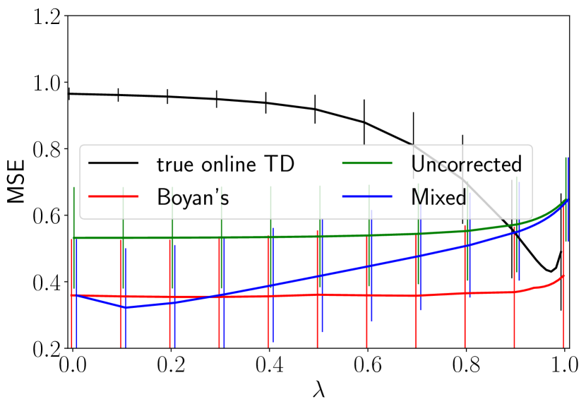
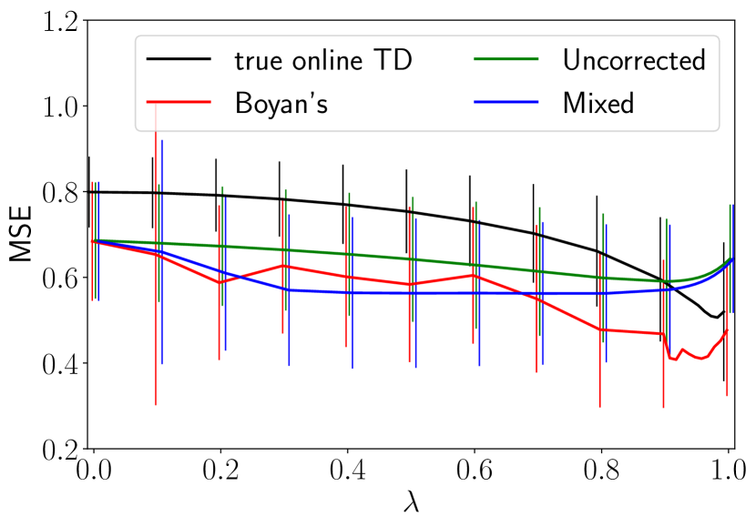
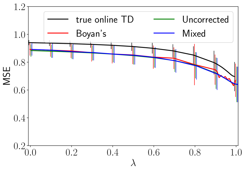
large MRP $(100,10,0.1)$
 
 
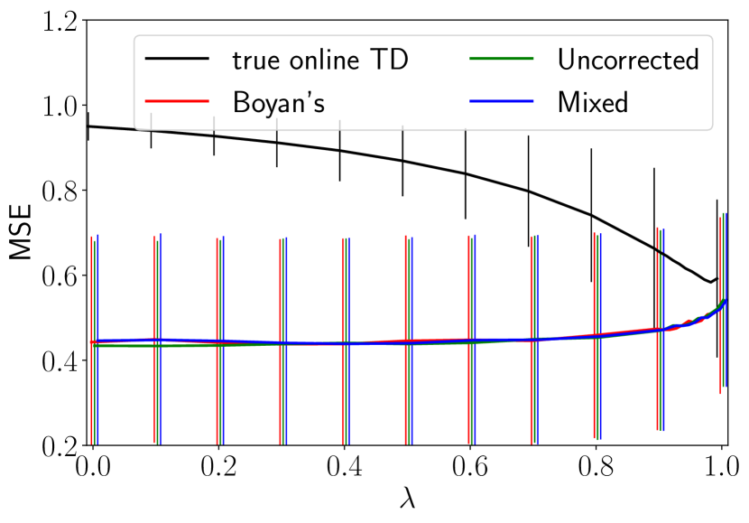
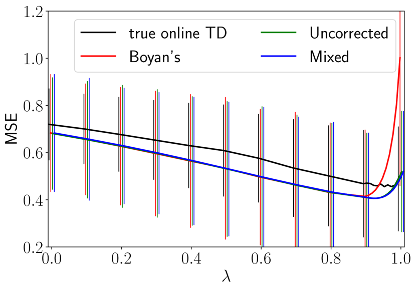
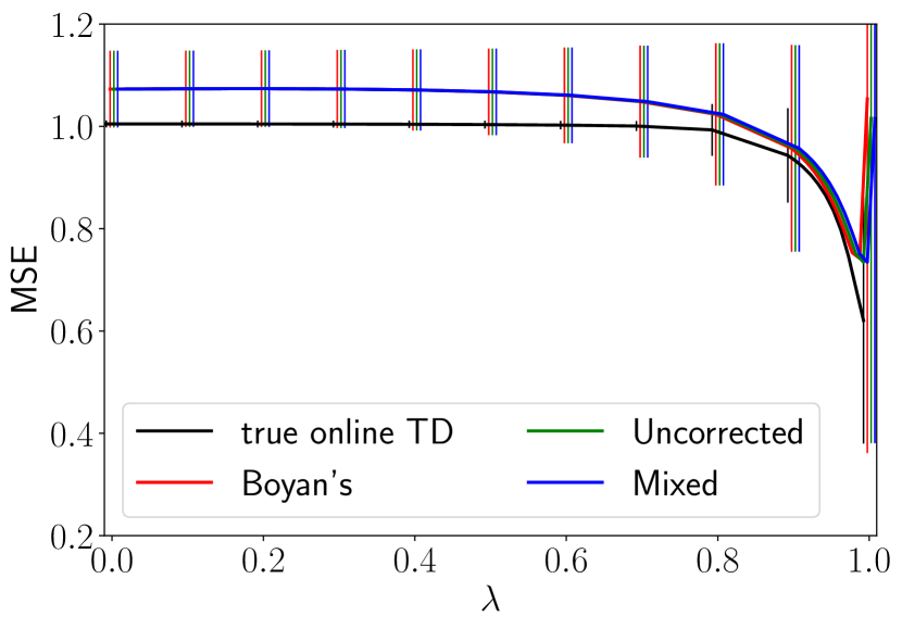
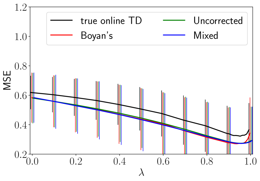
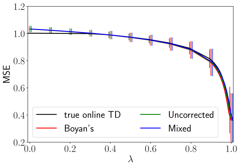
deterministic MRP $(100,3,0)$
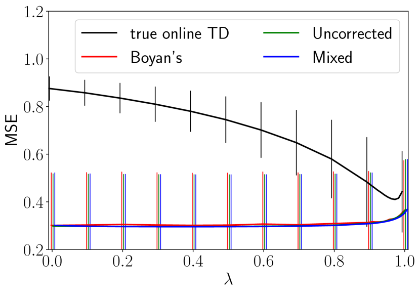
(a) tabular features (b) binary features (c) non-binary features

Figure 2: Mean squared error (MSE) of Uncorrected, Mixed, and Boyan’s LSTD($\lambda$) as well as true online TD($\lambda$). The MSE is evaluated on three random Markov reward processes (MRPs), each with three representations (features) of states. For Uncorrected, Mixed, and Boyan’s LSTD($\lambda$), the best MSE with the optimal value of regularization coefficient (among $\{2^{i}\mid i=-8,-7,\ldots,7,8\}$) is shown for each $\lambda$. For true online TD($\lambda$), the best MSE with the optimal step size (see van Seijen et al. (2016) for details) is shown for each $\lambda$. For each data point, MSE is computed on the basis of 50 runs, and the error bar shows its standard deviation. For clarity, we show error bars only at $\lambda=i/10$ for $i=0,\ldots,9,10$.

Figure 2 shows the best achievable MSE with the optimal choice of hyperparameters for each LSTD($\lambda$) and for true online TD($\lambda$), but this best achievable MSE cannot be achieved in practice, because one cannot optimally tune the hyperparameters.

Figure 2 thus needs to be understood with the sensitivity of the performance to the particular values of hyperparameters, which are shown in Figures 3-5. These figures may be compared against Figures 10-12 of van Seijen et al. (2016). Note, however, that the horizontal axis is regularization coefficient in Figures 3-5 but step size in Figures 10-12 of van Seijen et al. (2016).

Table 1 shows the computational time (in seconds) of each LSTD($\lambda$) in each run of the experiment with the small MRP shown with Figure 3. Likewise, Tables 2-3 show the computational time with the large and deterministic MRPs shown with Figures 4-5. Notice that each run consists of $17\times 20=340$ combinations of the values of $\alpha$ and $\lambda$ (recall that we vary $\alpha$ in $\{2^{i}\mid i=-8,-7,\ldots,7,8\}$ for each of $\lambda$ in $\{i/100\mid i=0,10,\ldots,90,91,\ldots,100\}$). As a reference, we also include the running time of true online TD($\lambda$) on our environment. Because true online TD($\lambda$) considers $30\times 20=600$ combinations of the values of hyperparameters as in van Seijen et al. (2016), the running time is normalized by $340/600$ after running all of the combinations for fair comparison.

In our implementation, Uncorrected LSTD($\lambda$) requires slightly more computational time than Boyan’s, because at each step Uncorrected LSTD($\lambda$) copies and stores the eligibility trace to be used in the next step. As is expected, Mixed LSTD($\lambda$) requires (20 % to 65 %) more computational time than the other LSTD($\lambda$)s, because Mixed LSTD($\lambda$) applies the rank-one update twice.

Detailed results with the small MRP

Mixed LSTD($\lambda$)

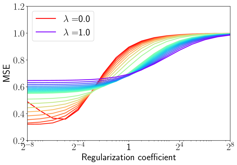
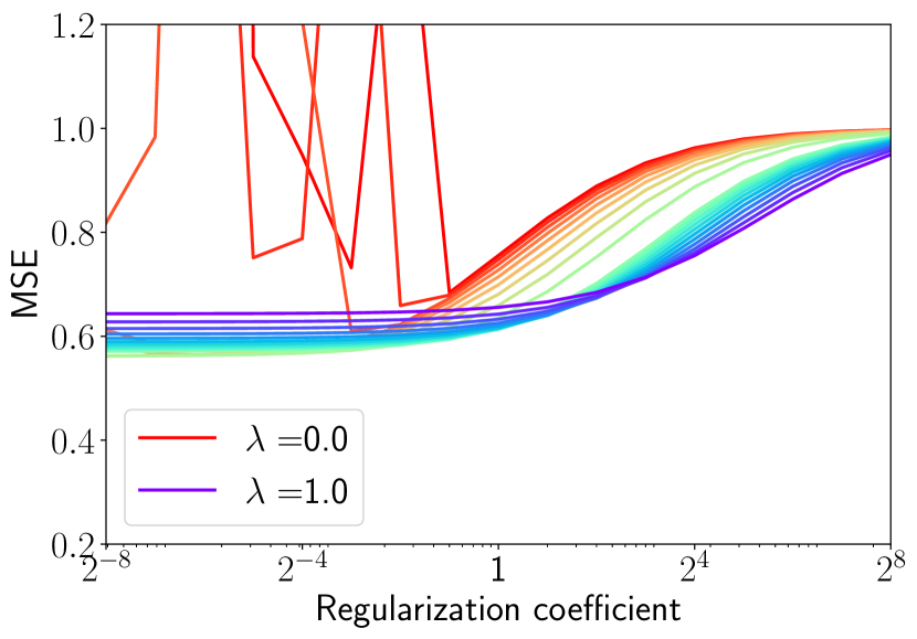
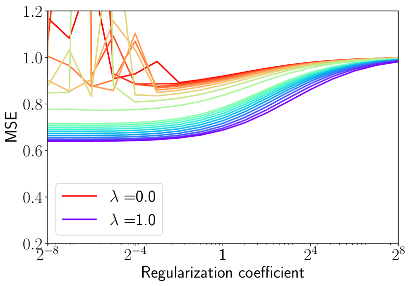
Uncorrected LSTD($\lambda$)

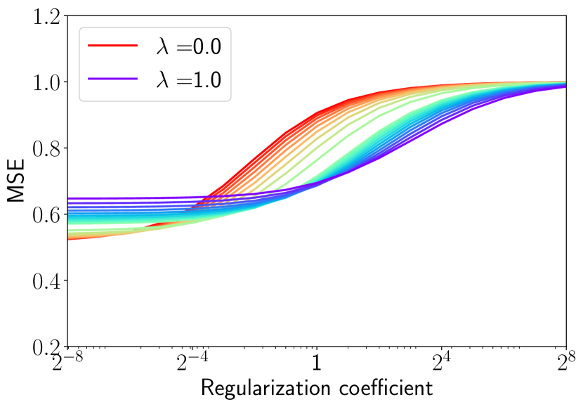
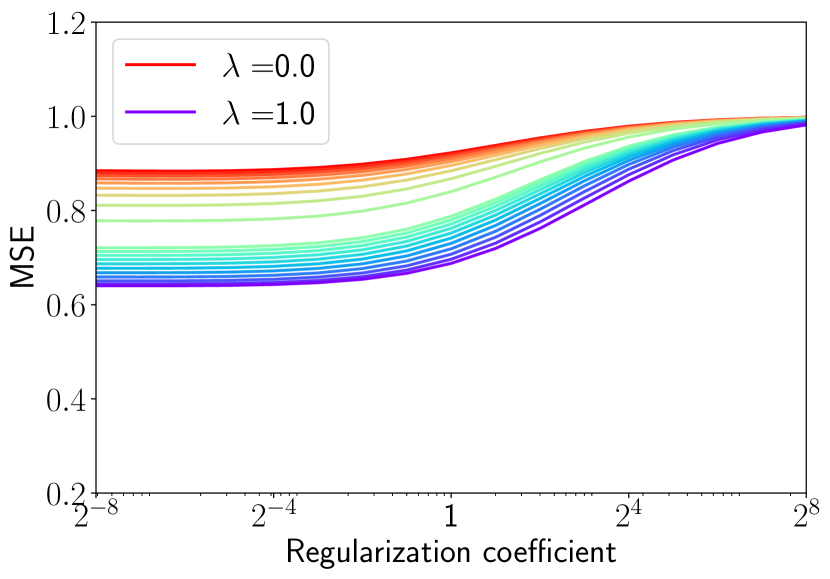
Boyan’s LSTD($\lambda$)

(a) tabular features

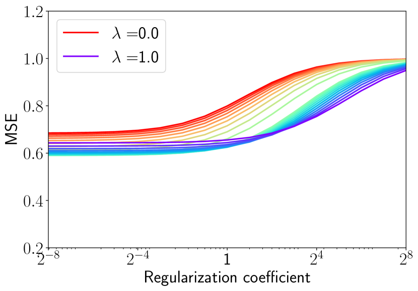
(b) binary features

(c) non-binary features

Figure 3: Mean squared error (MSE) of Uncorrected, Mixed, and Boyan’s LSTD($\lambda$) on the small MRP $(10,3,0.1)$ as a function of the value of regularization coefficient. Each curve shows the MSE (over 50 runs) of a particular value of $\lambda$ for $0\leq\lambda\leq 1$. The legend only shows the color with $\lambda\in\{0,1\}$, but the intermediate values of $\lambda$ follow the color map of rainbow. This figure is analogous to Figure 10 from van Seijen et al. (2016), but here we vary the value of regularization coefficient, while the step size is varied in van Seijen et al. (2016).

	Boyan’s	Uncorrected	Mixed	true online TD($\lambda$)
tabular	$1.10\pm 0.01$	$1.24\pm 0.01$	$1.49\pm 0.01$	$1.21\pm 0.01$
binary	$1.54\pm 0.01$	$1.72\pm 0.03$	$2.11\pm 0.03$	$1.87\pm 0.03$
non-binary	$1.54\pm 0.03$	$1.73\pm 0.01$	$2.13\pm 0.02$	$1.88\pm 0.01$

Table 1: The average computational time (seconds) for each run, consisting of 340 combinations of the values of hyperparameters, in the experiments with the small MRP. Here, the computational time of true online TD($\lambda$) is normalized by $340/600$ after running all of the 600 combinations of the values of hyperparameters.

Detailed results with the large MRP

Mixed LSTD($\lambda$)

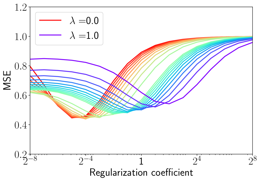
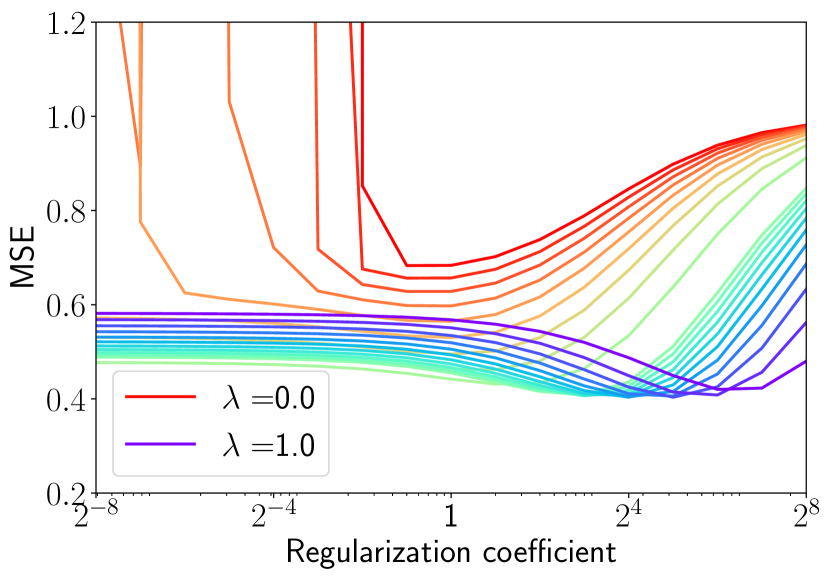
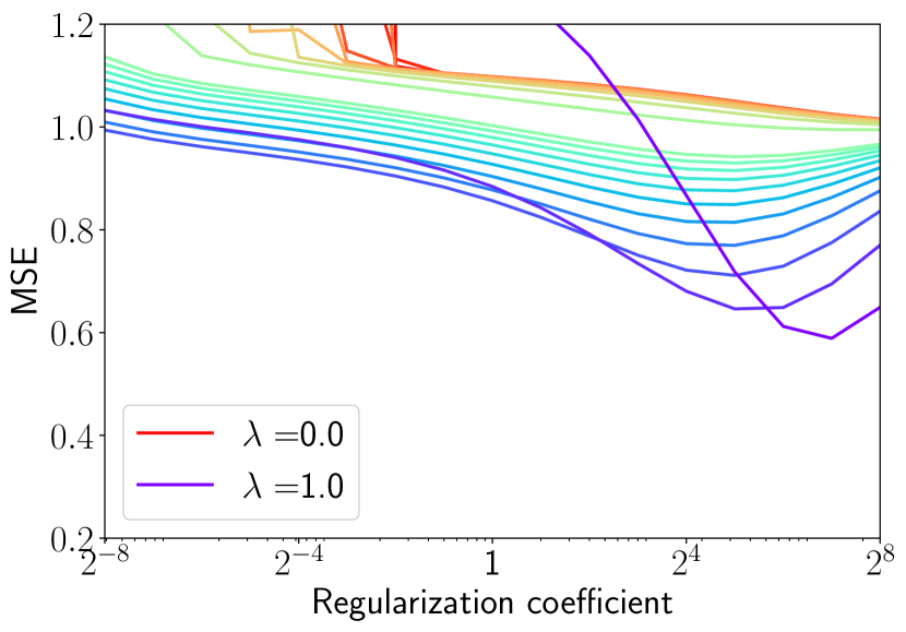
Uncorrected LSTD($\lambda$)

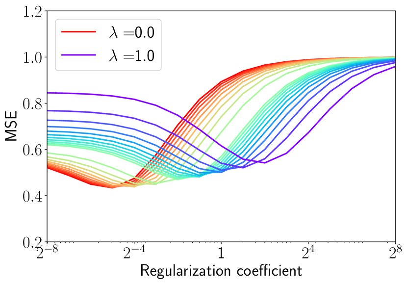
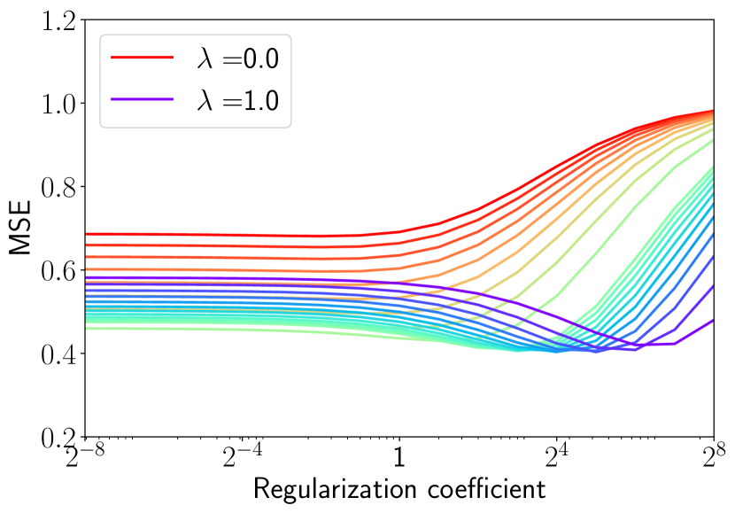
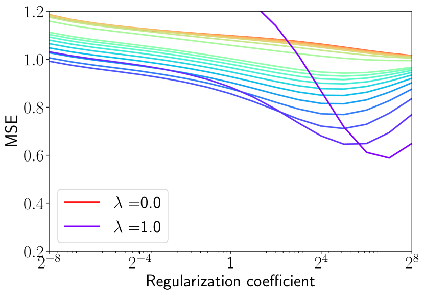
Boyan’s LSTD($\lambda$)

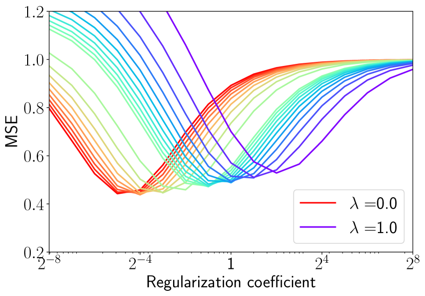
(a) tabular features

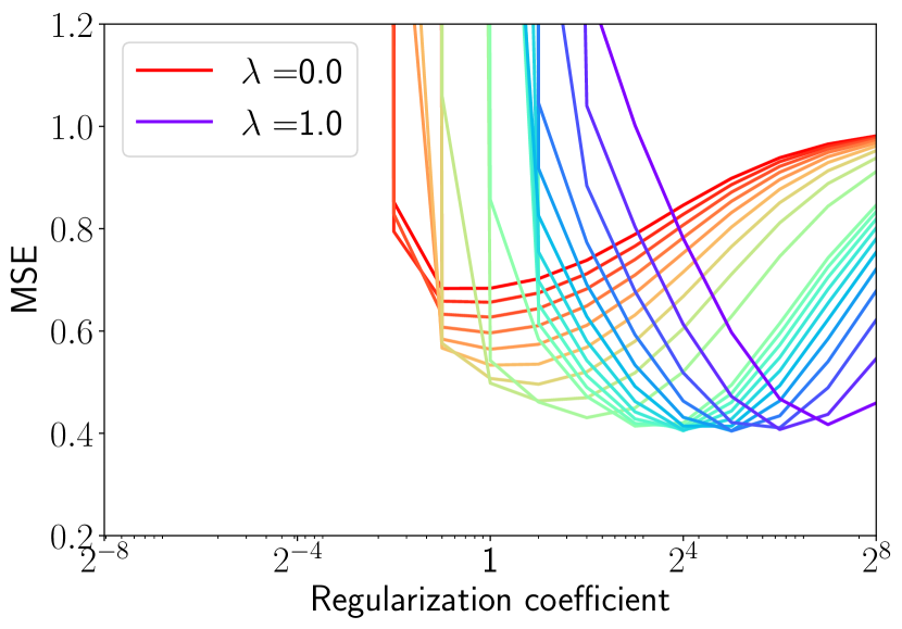
(b) binary features

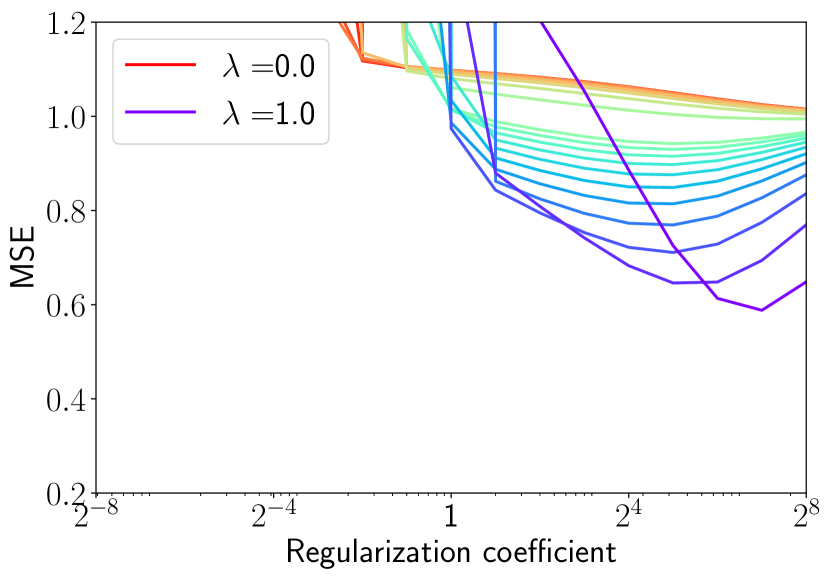
(c) non-binary features

Figure 4: Mean squared error (MSE) of Uncorrected, Mixed, and Boyan’s LSTD($\lambda$) on the large MRP $(100,10,0.1)$ as a function of the value of regularization coefficient. See the caption of 3 for the settings of experiments.

	Boyan’s	Uncorrected	Mixed	true online TD($\lambda$)
tabular	$27.1\pm 0.6$	$29.5\pm 0.4$	$44.7\pm 1.0$	$21.3\pm 0.2$
binary	$15.8\pm 0.1$	$17.7\pm 0.1$	$22.1\pm 0.4$	$19.8\pm 0.2$
non-binary	$15.7\pm 0.3$	$17.3\pm 0.1$	$21.9\pm 0.3$	$19.8\pm 0.3$

Table 2: The average computational time (seconds) for each run in the experiments with the large MRP. See the caption for Table 1 for details.

Detailed results with the deterministic MRP

Mixed LSTD($\lambda$)

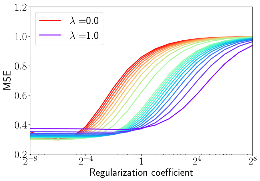
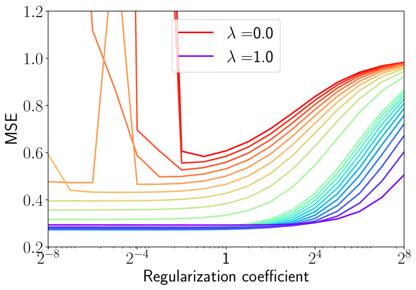
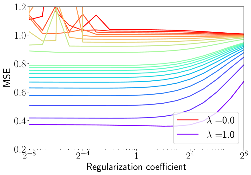
Uncorrected LSTD($\lambda$)

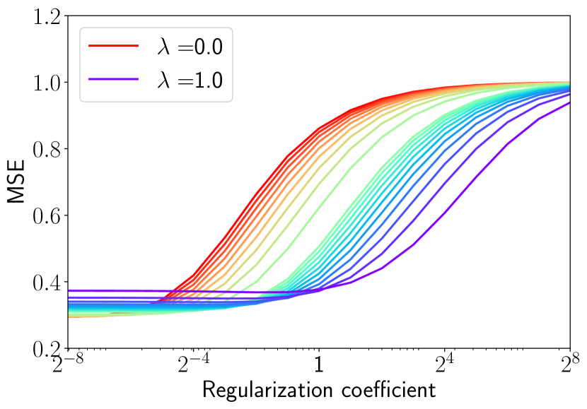
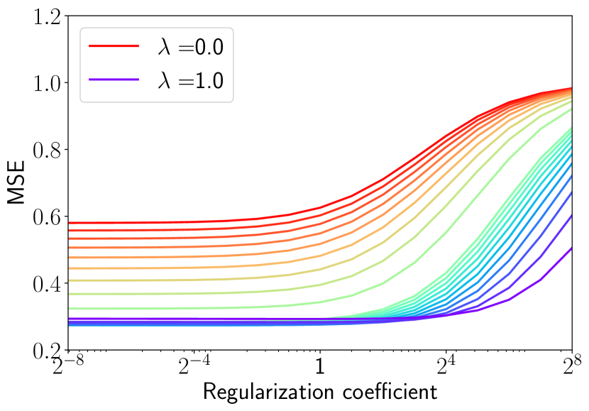
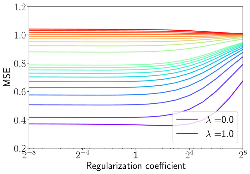
Boyan’s LSTD($\lambda$)

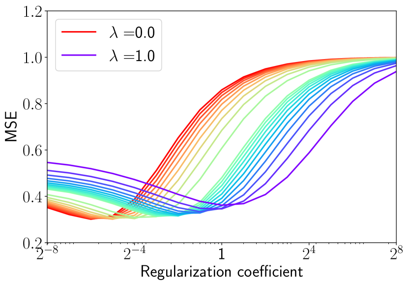
(a) tabular features

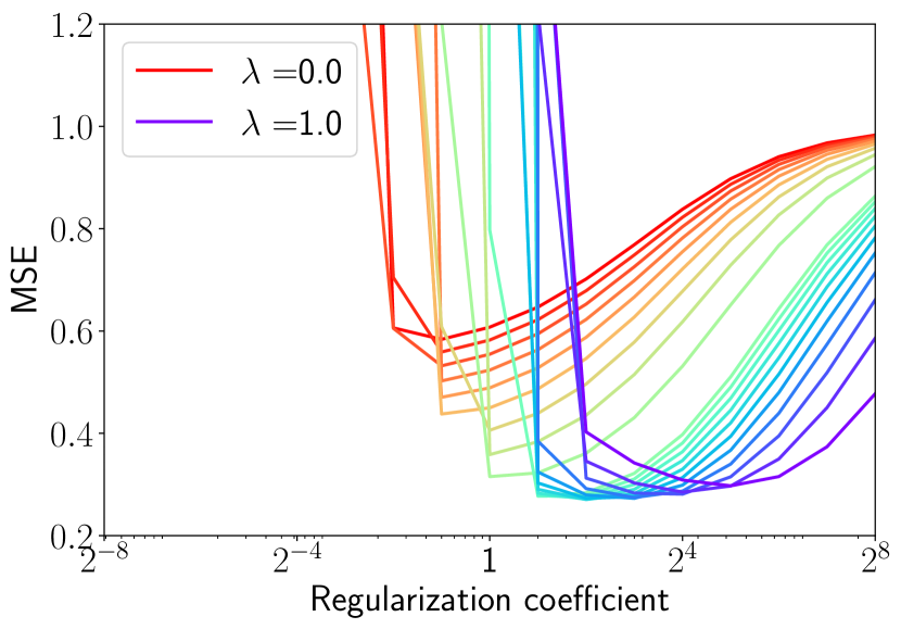
(b) binary features

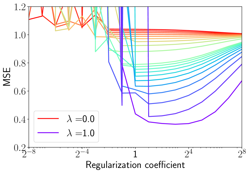
(c) non-binary features

Figure 5: Mean squared error (MSE) of Uncorrected, Mixed, and Boyan’s LSTD($\lambda$) on the deterministic MRP $(100,3,0)$ as a function of the value of regularization coefficient. See the caption of 3 for the settings of experiments.

	Boyan’s	Uncorrected	Mixed	true online TD($\lambda$)
tabular	$26.6\pm 0.3$	$28.6\pm 0.3$	$43.6\pm 0.6$	$19.9\pm 0.2$
binary	$14.8\pm 0.2$	$16.2\pm 0.1$	$21.4\pm 0.3$	$18.4\pm 0.4$
non-binary	$14.5\pm 0.2$	$16.3\pm 0.1$	$21.0\pm 0.2$	$18.7\pm 0.2$

Table 3: The average computational time (seconds) for each run in the experiments with the deterministic MRP. See the caption for Table 1 for details.

References

- Osogami (2019) T. Osogami. Uncorrected least-squares temporal difference with lambda-return. In Proceedings of the 34th AAAI Conference on Artificial Intelligence, February 2019.
- van Seijen et al. (2016) H. van Seijen, A. R. Mahmood, P. M. Pilarski, M. C. Machado, and R. S. Sutton. True online temporal-difference learning. Journal of Machine Learning Research, 17(145):1–40, 2016.