Velocity and Speed Correlations in Hamiltonian Flocks

Abstract

We study a $2d$ Hamiltonian fluid made of particles carrying spins coupled to their velocities. At low temperatures and intermediate densities, this conservative system exhibits phase coexistence between a collectively moving droplet and a still gas. The particle displacements within the droplet have remarkably similar correlations to those of birds flocks. The center of mass behaves as an effective self-propelled particle, driven by the droplet’s total magnetization. The conservation of a generalized angular momentum leads to rigid rotations, opposite to the fluctuations of the magnetization orientation that, however small, are responsible for the shape and scaling of the correlations.

Flocking, the formation of compact groups of collectively moving individuals, is a hallmark of animal group behavior. This phenomenon has long attracted the interest of biologists Breder Jr. (1954); Aoki (1982); Badgerow (1988); Huth and Wissel (1992); Krause and Ruxton (2002); Tunstrøm et al. (2013); Rosenthal et al. (2015), and motivated a large number of theoretical studies, connecting microscopic Vicsek like models Vicsek et al. (1995); Grégoire and Chaté (2004); Vicsek and Zafeiris (2012) to continuous theories of the Toner-Tu type Toner and Tu (1995); Tu et al. (1998); Toner et al. (2005); Peshkov et al. (2014); Marchetti et al. (2013); Yang and Marchetti (2015). On the experimental side, most quantitative data were obtained in artificial systems Schaller et al. (2010); Deseigne et al. (2010); Bricard et al. (2013); Geyer et al. (2018). One noticeable exception is the large scale observational and data analysis effort conducted by the Starflag project Cavagna et al. (2010, 2013); Attanasi et al. (2014); Hemelrijk and Hildenbrandt (2015); Attanasi et al. (2015); Cavagna et al. (2018, 2019a): the individual three-dimensional trajectories of a few thousand birds in compact flocks were obtained and studied. In particular, the starling flocks display correlations for the bird speeds and velocities that have been described as long-ranged and scale-free Cavagna et al. (2010, 2019a).

The study of collective motion in vibrated polar grains Deseigne et al. (2012); Weber et al. (2013) showed that considering the particles’ headings and their velocities as distinct, but coupled, degrees of freedom was instrumental to model the experimental observations Deseigne et al. (2010); Scholz et al. (2018). It was soon noticed that, under such coupling, the existence of collective motion in equilibrium cannot be ruled out by standard arguments. A Hamiltonian model of particles carrying ferro-magnetically coupled spins, that also interact with their own velocities, was then proposed Bore et al. (2016). Such model exhibits collectively moving polar ground states at temperature $T=0$ (in finite size systems) Bore et al. (2016),

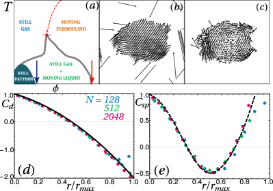
Figure 1: Hamiltonian flocks. $(a)$ Sketch of the phase diagram in the ($\phi,T$) plane, for small $K$ and $N$. The red and blue arrows indicate the densities studied here, $\phi=0.55$ and $\phi=0.14$. $(b)-(c)$ Snapshots of the displacements and their fluctuations within a flock ($N=512,K=0.03,T=10^{-2}$). $(d)-(e)$ Spatial correlations $C_{d}$ (resp. $C_{sp}$) of the displacement (resp. the speed) fluctuations, against distance normalized by the typical droplet size, for three system sizes ($T=10^{-2}$). The black lines are our theoretical predictions.

and a rich phase diagram at finite $T$ Casiulis et al. (2020), Fig. 1(a), with coexistence between a magnetized moving droplet and a disordered still gas, see Figs. 1(b)-(c) and Movie1.mp4 in the SI.

In this Letter, we show that the velocities and speeds of the particles inside the moving droplet exhibit correlations that are very similar to those observed in bird flocks, Figs. 1(d)-(e). Analyzing the evolution in the homogeneous polar and moving droplet phases, we show that the dynamics of the center of mass are the ones of an effective self-propelled particle, driven by the droplet magnetization. The spontaneous fluctuations of the magnetization, together with the conservation of a generalized angular momentum, induce a rigid body rotation of the droplet which, we show, is responsible for the form and scaling of the displacement correlations. We conclude by discussing the relevance of our findings for real bird flocks.

Our model, first introduced in Bore et al. (2016), consists in a system of $N$ particles, in a 2d periodic square box of linear size $L_{0}$, interacting through an isotropic short-range repulsive potential $U(r)=4(1-r)^{4}\Theta(1-r)$, with $\Theta$ the Heaviside step function. Each particle carries a unit planar vector, or spin, ${\bm{s}}_{i}$, with continuous orientation. The spins are coupled ferro-magnetically through an isotropic short-range coupling $J(r)=(1-r)^{2}\Theta(1-r)$. This ferromagnetic interaction induces an effective attraction at low temperature, $T$, resulting in an effective hard radius $r_{0}=1/4$ at $T=0$. We define the packing fraction $\phi\equiv\pi Nr_{0}^{2}/L_{0}^{2}$. The key ingredient is the introduction of a self-alignment between the spin and the velocity of each particle, through a coupling constant $K$. Starting from the Lagrangian formulation (see the SI), we obtain:

$$\mathcal{H} \!=\!\!\sum\limits_{i=1}^{N}\!\left(\frac{\bm{p}_{i}^{2}}{2}\!+\!\frac{\omega_{i}^{2}}{2}-K\bm{p}_{i}\!\cdot\!\bm{s}_{i}\right)\!+\!\frac{1}{2}\sum\limits_{k\neq i}\!\left[U(r_{ik})\!-\!J(r_{ik})\,\bm{s}_{i}\!\cdot\!\bm{s}_{k}\right]$$ (1)

where ${\bm{r}_{i}}$ are the positions of the particles, $r_{ik}=|{\bm{r}}_{i}-{\bm{r}}_{k}|$, ${\bm{s}_{i}}$ their spins parametrized by an angle $\theta_{i}$, $\omega_{i}=\dot{\theta_{i}}$ the momenta associated to these angles, and $\bm{p}_{i}=\dot{\bm{r}}_{i}+K\bm{s}_{i}$ the linear momenta associated to the positions.

The dynamics conserve the total energy $\mathcal{H}$, the total linear momentum $\bm{P}=\sum_{i}\bm{p}_{i}=N(\bm{v}_{G}+K\bm{m})$, and the total angular momentum $\bm{L}=\sum_{i}\left[\omega_{i}\hat{\bm{e}}_{z}+\bm{r}_{i}\times\bm{v}_{i}+K\bm{r}_{i}\times\bm{s}_{i}\right]$, where $\bm{v}_{G}=N^{-1}\sum_{i}\dot{\bm{r}}_{i}$ is the center of mass velocity, $\bm{m}=N^{-1}\sum_{i}\bm{s}_{i}$ is the intensive magnetization, and $\hat{\bm{e}}_{z}=\hat{\bm{e}}_{x}\times\hat{\bm{e}}_{y}$ is the out-of-plane unit vector. We perform Molecular Dynamics (MD) simulations in the $(N,V,E)$ ensemble, using initial conditions such that $\bm{P}=\bm{L}=\bm{0}$. For $K=0$, and at sufficiently low packing fraction, $\phi$, and temperature, $T$, the system undergoes a ferromagnetism-induced phase separation (FIPS) between a ferromagnetic liquid and a paramagnetic gas due to the emergence of an effective attraction generated by the tendency of the spins to align Casiulis et al. (2019). For $K>0$, a similar phase separation is observed Casiulis et al. (2020) (see also the SI). The conservation of momentum imposes that magnetized phases move collectively with velocity $\bm{v}_{G}=-K\bm{m}$. As a result, for large values of $N$ or $K$, the high kinetic energy cost of the polar moving states prohibits the existence of magnetized phases, and still patterns, such as vortices or solitons, with locally aligned spins but no global magnetization, emerge Casiulis et al. (2020). On the contrary, for small enough $K$ and $N$, the system maintains its magnetization, and spontaneously develops a mean velocity for a wide range of $\phi$ and $T$, see Fig. 1(a). In the following we focus on this last situation.

In the coexistence regime, the moving phase consists in a moving droplet, surrounded by a still gas. Figure 1(b) displays a typical snapshot of the displacements $\bm{u}_{i}\equiv\bm{r}_{i}(\tau)-\bm{r}_{i}(0)$, where $\tau=2\cdot 10^{2}$, is chosen long enough to average out thermal fluctuations and reach a limit in which the correlations are $\tau$ independent (see SI). One can observe the strong polarization of the displacements inside the droplet; their polarity, as defined in the context of bird flocks Cavagna et al. (2010); Hemelrijk and Hildenbrandt (2015) is $\Phi\equiv N^{-1}\left|\sum_{i}\bm{u}_{i}/\left|\bm{u}_{i}\right|\right|\simeq 0.95$. More intriguing are the displacement fluctuations, $\bm{u}_{i}^{\star}\equiv\bm{u}_{i}-\bm{u}_{G}$, where $\bm{u}_{G}=N^{-1}\sum_{k}\bm{u}_{k}$, displayed in Fig. 1(c). They present a clear spatial organization, which we quantify by computing their spatial correlations across the flock:

$$C_{d}(r)=\frac{1}{c_{0}}\frac{\sum\limits_{j\neq i}\bm{u}^{\star}_{i}\cdot\bm{u}^{\star}_{j}\delta(r-r_{ij})}{\sum\limits_{j\neq i}\delta(r-r_{ij})}\;.$$ (2)

with $\delta$ a binning function  and $c_{0}$ fixing $C_{d}(0)=1$. Similarly, one defines the speed-speed correlation, $C_{sp}(r)$, by replacing $\bm{u}_{i}^{\star}$ by $\left|\bm{u}_{i}\right|-N^{-1}\sum\left|\bm{u}_{k}\right|$ in the above definition. Figure 1(d)-(e) display $C_{d}(r)$ and $C_{sp}(r)$ against $r/r_{max}$ for $N=128,512,2048$ and $K=0.03,0.03,0.001$, respectively, with $r_{max}$ the largest distance between two particles in the droplet. We observe an excellent data collapse, indicating that the only relevant scale is the droplet size.

Such correlations, without any scale other than the system size, were first reported in bird flocks Cavagna et al. (2010). In the theoretical framework of the Vicsek model Vicsek et al. (1995) and its hydrodynamic description by Toner-Tu Toner and Tu (1995); Tu et al. (1998); Toner et al. (2005), in which flocking results from the build-up of a true long-range polar order, these correlations have been described as being scale-free, suggesting an underlying critical phenomenon. Yet, as stated in Ref. Cavagna et al. (2010), while the hydrodynamic theories of flocking are good candidates to explain the correlations of the displacement vectors, in particular the ones of their orientations, they do not explain the scale-free nature of the speed correlations. Explaining the latter within a critical framework requires either the application of an external dynamical field Cavagna et al. (2013), or the introduction of a free energy with a marginal direction Cavagna et al. (2019a).

Although it is clear that the present model is not a model of birds, with metric instead of topological interactions which induce structural features absent in flocks Cavagna et al. (2008); Ballerini et al. (2008), the fact that we recover strikingly similar correlations suggests the possible contribution of yet another source of correlations, which we shall now unveil.

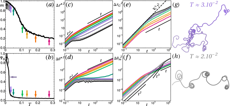
Figure 2: Dynamics and Structure of the Homogeneous phases across the Curie line and hexatic transition. $(a)$ Mean magnetization modulus and $(b)$ hexatic order parameter versus $T$. The arrows indicate the $T$ values at which the MSD curves in $(c)-(f)$ are recorded. $(c)$ MSD and $(d)$ MSAD of the relative displacements versus time, in log-log scale. $(e)$ MSD of the center of mass (the dashed black line indicates $v_{G}=K$), and $(f)$ MSAD of the magnetization vector versus time, in log-log scale. $(g)-(h)$ Trajectories of the center of mass, with time going from light to dark, for two temperatures corresponding to the $(g)$ mauve and $(h)$ light gray curves in $(c)-(f)$. $N=128,K=0.23$, $\phi=0.55$ (red arrow in Fig. 1$(a)$).

We start with a quantitative description of the structure and dynamics of the homogeneous moving phase, and then we focus on the inhomogeneous one. To address the first case, we choose $\phi=0.55$ (orange arrow in Fig. 1(e)) with $N=128$ and $K=0.23$. When decreasing the temperature, the system first magnetizes (Fig. 2(a)) at a crossover taking place at $T\approx 10^{-1}$. At even lower $T$ ($T\leq 2\cdot 10^{-2}$) a structural organization takes place, as testified by the growth of the hexatic order parameter $\Psi_{6}$ Halperin and Nelson (1978), symptomatic of a 2d system approaching a solid phase (Fig. 2(b)). The dynamics are then characterized for a few values of $T$, indicated by arrows in Fig. 2(a)-(b). The relative Mean Square Displacements (MSD), ${\Delta r^{\star}}^{2}(t)$, shown in Fig. 2(c) are the ones of a usual fluid: they cross over from a short-time ballistic regime to a long-time diffusive one, and feature finite plateaus at low $T$s, revealing the freezing of the dynamics as the system becomes solid van Megen et al. (1998); Sánchez-Miranda et al. (2015). The Mean Square Angular Displacements (MSAD) associated to the spin fluctuations around the mean magnetization, ${\Delta\theta^{\star}}^{2}(t)$ shown in Fig. 2(d), behave like the MSD, except that the plateaus develop at the magnetization crossover: spin-wave excitations are exponentially suppressed as the temperature decreases Tobochnik and Chester (1979), similarly to what we found for $K=0$ Casiulis et al. (2019). The MSD associated to $\bm{u}_{G}$, $\Delta r_{G}^{2}(t)$, or “center-of-mass” MSD, characterizes the collective motion of the fluid (Fig. 2(e)). At short times the motion is ballistic, with a collective speed $v_{G}=Km$ due to momentum conservation. At long times it becomes diffusive, with a diffusion coefficient that grows as $T$ decreases. At very low $T$, one notices the presence of a short sub-diffusive regime, which separates the ballistic from the diffusive regime. Finally, the MSAD $\Delta\theta_{m}^{2}(t)$ associated to the orientation of the magnetization, $\theta_{m}=\text{atan}(m_{y}/m_{x})$ (Fig. 2(f)) is ballistic at short times, showing that the magnetization follows inertial dynamics, and diffusive at long times, with a diffusion constant which decreases with decreasing $T$ as long as the system is paramagnetic, and increases when further decreasing $T$ into the ferromagnetic phase. At very low $T$, and unusual intermediate super-ballistic regime develops at the liquid-solid crossover, concomitantly with the sub-diffusive regime of $\Delta r_{G}^{2}$. The trajectories of the center of mass give a first hint of its origin. In the isotropic liquid, Fig. 2(g), the trajectories look like persistent random walks whereas, as the system rigidifies, Fig. 2(h), loops with accelerated rotations of $\bm{m}$ appear, leading to a less efficient exploration of space.

The role played by the onset of rigidity can be rationalized, writing down an effective model for the dynamics of the center of mass. We recall that the angular momentum is conserved. Decomposing the positions, spins and velocities as $\bm{r}_{i}=\bm{r}_{G}+\bm{r}_{i}^{\star}$, $\bm{s}_{i}=\bm{m}+\bm{\delta s}_{i}$ and $\bm{v}_{i}=-K\bm{m}+r_{i}^{\star}\Omega\hat{\bm{e}}_{\phi,i}+\bm{\delta v}_{i}$, with $\Omega$ the mean rotational velocity and $\hat{\bm{e}}_{\phi,i}=\hat{\bm{e}}_{z}\times\bm{r}_{i}/r_{i}$, and using that $\bm{P}=\bm{0}$, the angular momentum reads

$$\bm{L}=N\dot{\theta}_{m}\hat{\bm{e}}_{z}+I\Omega\hat{\bm{e}}_{z}+\bm{\delta L}\;,$$ (3)

where $I=\sum r_{i}^{2}$ is the moment of inertia, and $\bm{\delta L}=\sum\bm{r}_{i}^{\star}\times(\bm{\delta v}_{i}+K\bm{\delta s}_{i})$. Assuming that $\Omega\approx f\dot{\theta}_{m}$, with $f$ a constant, approximating $\bm{\delta\dot{L}}$ by a noise term, and introducing a characteristic time $\tau_{m}\sim(N+fI)/(f\dot{I})$, that we treat as a constant, the conservation law $\dot{\bm{L}}=\bm{0}$ reads

$$\tau_{m}\ddot{\theta}_{m}+\dot{\theta}_{m} =\sqrt{D_{r}}\eta_{m}\;,$$ (4)

where $D_{r}$ is a rotational diffusion constant, and $\eta_{m}$ a centered Gaussian white noise. All in all, neglecting for simplicity the fluctuations of the magnetization amplitude, the dynamics of the center of mass obey the equation $\bm{v}_{G}=-Km(T)\hat{\bm{e}}_{\bm{m}}$ where $\hat{\bm{e}}_{\bm{m}}$, the orientation of $\bm{m}$, follows the dynamics prescribed by Eq. (4).

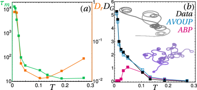
Figure 3: AVOUP Dynamics. $(a)$ $\tau_{m}$ (green) and $D_{r}$ (orange) versus $T$ in lin-log scale. $(b)$ $D_{G}$ against $T$ (black), together with the ABP (red) and AVOUP (blue) estimations. Inset: Trajectories, with time going from light to dark, obtained by integrating the AVOUP equations of motion over $t=10000$, with an integration step $\delta t=1$, and fixed values $Km=0.1,D_{r}=1$. $\tau_{m}=5000$ (gray), and $\tau_{m}=500$ (mauve).

This equation states that $\theta_{m}$ is subject to inertia and rotational diffusion and defines an Angular Velocity Ornstein-Uhlenbeck Particle (AVOUP) process, a model similar to the ones used to describe experimental living systems, ranging from microtubules to flatworms Sumino et al. (2012); Nagai et al. (2015); Chen et al. (2017); Sugi et al. (2019). Here, the inertial time $\tau_{m}$ not only grows as the moment of inertia increases, but also as the deformation dynamics (encoded by $\dot{I}$) are suppressed: in other words, it increases as the system becomes rigid. The associated accelerated dynamics of $\theta_{m}$ is responsible for the super-ballistic regime observed for $\Delta\theta_{m}(t)$ and, in turn, the sub-diffusive regime for $\Delta r_{G}(t)$. In fact, the large inertia limit, $\tau_{m}\to\infty$, yields a random-acceleration process, that behaves like $\Delta\theta_{m}^{2}\sim t^{3}$ at long times Burkhardt (2007). This regime was related to looping trajectories in a study of self-propulsion with memory Kranz and Golestanian (2019). We further validate our effective description by comparing the diffusion constant of the center of mass, $D_{G}$, obtained from the MD simulations, with the theoretical prescription for AVOUP Ghosh et al. (2015):

$$D_{G}^{\rm AVOUP} =D_{G}^{\rm ABP}\Gamma(\tau_{m}D_{r})\sum\limits_{n=0}^{\infty}\frac{(\tau_{m}D_{r})^{n+1}}{\Gamma(n+1+\tau_{m}D_{r})}\;,$$ (5)

where we introduced the $\Gamma$-function and $D_{G}^{\rm ABP}=K^{2}m^{2}/(2D_{r})$ is the diffusion constant in the over-damped limit of Active Brownian Particles (ABP) Fily and Marchetti (2012); Winkler et al. (2015). We extract $D_{r}$ from the long-time diffusive behavior of $\theta_{m}$, and $\tau_{m}$ from a short-time exponential fit of the two-time autocorrelation $C(t)=\langle\dot{\theta}_{m}(0)\dot{\theta}_{m}(t)\rangle$. These inputs are plotted against $T$ in Fig. 3(a). Note that $\tau_{m}$ rises concomitantly with $\Psi_{6}$, confirming that the inertia of $\theta_{m}$ is tightly related to the rigidity of the system. Figure 3(b) shows how good the AVOUP estimation of $D_{G}$ is, while the zero-memory limit is essentially valid only at high $T$, where the magnetization is low. The trajectories obtained by integrating the AVOUP dynamics are also good reproductions of the ones shown in Fig. 2.

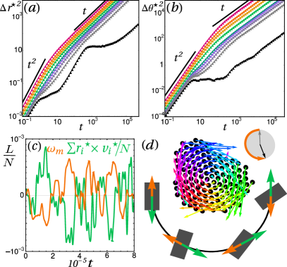
Figure 4: Spontaneous Rigid Rotations. Relative $(a)$ MSD and $(b)$ MSAD for $N=128,K=0.03,\,\phi\approx 0.14$ (blue arrow in Fig. 1$(a)$) and $T$ increasing from black to red. The coexistence line is crossed between the green and teal lines. $(c)$ Typical $\omega_{m}=\dot{\theta}_{m}$ (orange) and $N^{-1}\sum\bm{r}_{i}^{\star}\times\bm{v}_{i}^{\star}$ (green), time-averaged over $\tau_{w}=10^{2}$, versus time ($T\approx 10^{-2}$). $(d)$ Relative displacements color-coded according to their orientation and rescaled by their mean ($T\approx 10^{-2},\tau\approx 10^{4}$), together with a sketch of the spontaneous rotation dynamics ($\bm{m}$ in orange and $\bm{v}_{G}$ in green). Upper inset: the rotation of $\bm{m}$ from the gray to the black arrow, following the orange curved arrow.

Coming back to the phase-separated states, say at $\phi=0.14$, $N=128$, and $K=$ $0.03$, we observe that the AVOUP description and the general features of the center of mass trajectories are almost unchanged, see Fig. 4. The only major difference occurs at very low $T$, where the droplet is highly magnetized, structurally ordered, dynamically frozen, and immersed in a very low density gas. Under these circumstances, the relative displacements exhibit an intermediate second ballistic regime, that can also be explained by the conservation of ${\bm{L}}$. As an individual flock is free to rotate around its center of mass, a rotation of the magnetization must be compensated by either a rigid rotation in the opposite direction or thermal fluctuations [see Eq. (3)]. At very low $T$, the thermal fluctuations are no longer enough to absorb changes in $\dot{\theta}_{m}$. As a result, for $\bm{L}=\bm{0}$, the droplets develop rigid rotations such that $N\dot{\theta}_{m}=-I\Omega$, as confirmed when plotting time-averaged versions of $\dot{\theta}_{m}$ and $N^{-1}\sum\bm{r}_{i}^{\star}\times\bm{v}_{i}^{\star}$, Fig. 4(c). The associated displacement fields, Fig. 4(d), explain our initial observations, Fig. 1(d)-(e): a rigid rotation yields a correlation of the relative displacements at the scale of the size of the system (see also Movie2.mp4 in the SI). The excellent match between the numerically observed and analytical $C_{d}$ and $C_{sp}$ for a homogeneous rigid disk rotating at a constant rate (see the SI), shown with black lines in Fig. 1(d)-(e), confirms the above interpretation.

We showed that Hamiltonian flocks exhibit correlations remarkably similar to those observed in bird flocks, with no other scale than the droplet size. In the latter, the scaling and functional form of the correlations stem from rigid body rotations around the center of mass of the flock. Hence the question: in bird flocks, what is the part of the correlations due to, on the one hand, the Goldstone mode along the orthoradial direction of an effective potential ($C_{d}$) Cavagna et al. (2010) and the marginality of its radial direction ($C_{sp}$) Cavagna et al. (2019a) and, on the other hand, rotations? It is not obvious which effect is stronger. For physiological reasons, the rotations cannot be large Cavagna et al. (2018) but in an $O(n)$ model, the amplitude of the correlation scales like $1-m^{2}$, with $m$ the magnetization, and is thus also very small for well polarized systems like bird flocks Cavagna et al. (2010). To assess the importance of each effect, we analyze the data from the SI of Ref. Cavagna et al. (2010) (see SI): while the shape of $C_{d}$ is dominated by the spin wave contribution, $C_{sp}$ is controlled by the rigid body rotation. This deserves a few comments. First, a rotation of a fraction of a degree, compatible with the variability of bird speeds Cavagna et al. (2010), is sufficient to set the shape of $C_{sp}$. Second, although flocks do not turn via a rotation around an external point Cavagna et al. (2018), a small rotation around the center of mass is not precluded: in fact, a turn due to a spin wave generically contains a small, but finite rotation. Thus, while rigid rotations are not entirely responsible for velocity correlations in bird flocks, they may take part in them, and should not be overlooked. In particular, the variability in the shape of $C_{sp}$ across bird flocks Cavagna et al. (2019b) calls for a more systematic analysis.

Finally, we stress that, in Hamiltonian flocks, the rotation is rooted in the angular momentum conservation. Yet, rigid body rotations were also reported in systems with no strict angular momentum conservation, like self-propelled Janus colloids Ginot et al. (2018); van der Linden et al. (2019) and active dumbbells Petrelli et al. (2018). Whether the rotational invariance of active systems leads to pseudo-conserved generalized angular momenta remains to be elucidated.