An Invariant Test for Equality of Two Large Scale Covariance Matrices

Taehyeon Koo Seonghun Cho Johan Lim All authors are at Department of Statistics, Seoul National University, Seoul, Korea. Taehyeon Koo and Seonghun Cho equally contribute to the paper. All correspondence are to Johan Lim, E-mail:johanlim@snu.ac.kr.
Abstract

In this work, we are motivated by the recent work of Zhang et al. (2019) and study a new invariant test for equality of two large scale covariance matrices. Two modified likelihood ratio tests (LRTs) by Zhang et al. (2019) are based on the sum of log of eigenvalues (or 1- eigenvalues) of the Beta-matrix. However, as the dimension increases, many eigenvalues of the Beta-matrix are close to 00 or 111 and the modified LRTs are greatly influenced by them. In this work, instead, we consider the simple sum of the eigenvalues (of the Beta-matrix) and compute its asymptotic normality when all n1,n2,psubscript𝑛1subscript𝑛2𝑝n_{1},n_{2},p increase at the same rate. We numerically show that our test has higher power than two modified likelihood ratio tests by Zhang et al. (2019) in all cases both we and they consider.

Keywords: Equality of two covariance matrices, F-matrix, invariant test, linear spectral statistics, random matrix theory.

1 Introduction

We revisit the test of equality (homogeneity) of two covariance matrices, which often allows us simplified procedures for many multivariate problems. Suppose we have samples 𝐳i(l),i=1,2,,nl,formulae-sequencesuperscriptsubscript𝐳𝑖𝑙𝑖12subscript𝑛𝑙\mathbf{z}_{i}^{(l)},i=1,2,\ldots,n_{l}, from a distribution with a mean vector μlsubscript𝜇𝑙\mathbf{\mu}_{l} and covariance matrix ΣlsubscriptΣ𝑙\Sigma_{l} for l=1,2𝑙12l=1,2. The hypothesis, which is of interest, is

0:Σ1=Σ2versus1:Σ1Σ2.:subscript0subscriptΣ1subscriptΣ2versussubscript1:subscriptΣ1subscriptΣ2\mathcal{H}_{0}:\Sigma_{1}=\Sigma_{2}\quad\mbox{versus}\quad\mathcal{H}_{1}:\Sigma_{1}\neq\Sigma_{2}. (1)

As pointed out by Zhang et al. (2019), the history of the test draws back to 1930s and a huge number of works are followed in literature. In this paper, we do not aim to compete with all methods in the literature (see Chapter 10 of Anderson, T.W. (2003) and references therein). Instead, we focus on a specific invariant test as an alternative to the modified likelihood ratio test (mLRT), which is recently suggested by Zhang et al. (2019). In Section 2, we compute the asymptotic null distribution of the new test, when all n1,n2,psubscript𝑛1subscript𝑛2𝑝n_{1},n_{2},p increase at the same rate. In Section 3, we numerically show it has higher power than mLRT in all cases both we and they consider. In Section 4, we conclude the paper with some remarks.

2 An alternative invariant statistic

We find 𝐱il={xij(l)}superscriptsubscript𝐱𝑖𝑙superscriptsubscript𝑥𝑖𝑗𝑙\mathbf{x}_{i}^{l}=\{x_{ij}^{(l)}\}, for i=1,2,,nl,l=1,2formulae-sequence𝑖12subscript𝑛𝑙𝑙12i=1,2,\ldots,n_{l},l=1,2, where xijlsuperscriptsubscript𝑥𝑖𝑗𝑙x_{ij}^{l} are independent and identically distributed (IID) with mean zero and variance one, respectively, and satisfy

𝐳j(l)=Σl1/2𝐱j(l)+μl.superscriptsubscript𝐳𝑗𝑙superscriptsubscriptΣ𝑙12superscriptsubscript𝐱𝑗𝑙subscript𝜇𝑙\mathbf{z}_{j}^{(l)}=\Sigma_{l}^{1/2}\mathbf{x}_{j}^{(l)}+\mathbf{\mu}_{l}.

Let Sn1subscript𝑆subscript𝑛1S_{n_{1}} and Sn2subscript𝑆subscript𝑛2S_{n_{2}} be the sample covariance matrix from each population. To build our test, we focus on the limiting distribution of eigenvalues of 𝐁n=n1Sn1(n1Sn1+n2Sn2)1subscript𝐁𝑛subscript𝑛1subscript𝑆subscript𝑛1superscriptsubscript𝑛1subscript𝑆subscript𝑛1subscript𝑛2subscript𝑆subscript𝑛21\mathbf{B}_{n}=n_{1}S_{n_{1}}(n_{1}S_{n_{1}}+n_{2}S_{n_{2}})^{-1}, named as the limiting spectral distribution (LSD) of 𝐁nsubscript𝐁𝑛\mathbf{B}_{n}. With the notations

y1=p/n1,y2=p/n2,h=y1+y2y1y2,αn=n2/n1,formulae-sequencesubscript𝑦1𝑝subscript𝑛1formulae-sequencesubscript𝑦2𝑝subscript𝑛2formulae-sequencesubscript𝑦1subscript𝑦2subscript𝑦1subscript𝑦2subscript𝛼𝑛subscript𝑛2subscript𝑛1y_{1}=p/n_{1},y_{2}=p/n_{2},h=\sqrt{y_{1}+y_{2}-y_{1}y_{2}},\alpha_{n}=n_{2}/n_{1},

the limiting spectral distribution of 𝐁nsubscript𝐁𝑛\mathbf{B}_{n} is evaluated as (see Zhang et al. (2019))

𝐅γ1,γ2(x)=(α+1)(xrx)(xxl)2πy1x(1x)δx(xl,xr),subscript𝐅subscript𝛾1subscript𝛾2𝑥𝛼1subscript𝑥𝑟𝑥𝑥subscript𝑥𝑙2𝜋subscript𝑦1𝑥1𝑥subscript𝛿𝑥subscript𝑥𝑙subscript𝑥𝑟\mathbf{F}_{\gamma_{1},\gamma_{2}}(x)=\frac{(\alpha+1)\sqrt{(x_{r}-x)(x-x_{l})}}{2\pi y_{1}x(1-x)}\delta_{x\in(x_{l},x_{r})},

where xl,xr=y2(hy1)2(y1+y2)2,y1γ1,y2γ2formulae-sequencesubscript𝑥𝑙subscript𝑥𝑟subscript𝑦2superscriptminus-or-plussubscript𝑦12superscriptsubscript𝑦1subscript𝑦22formulae-sequencesubscript𝑦1subscript𝛾1subscript𝑦2subscript𝛾2x_{l},x_{r}=\frac{y_{2}(h\mp y_{1})^{2}}{(y_{1}+y_{2})^{2}},y_{1}\longrightarrow\gamma_{1},y_{2}\longrightarrow\gamma_{2} and αnαsubscript𝛼𝑛𝛼\alpha_{n}\longrightarrow\alpha as min{n1,n2,p}subscript𝑛1subscript𝑛2𝑝\min\{n_{1},n_{2},p\}\longrightarrow\infty.

Let Gn1,n2(x)=p(𝐅𝐁n(x)𝐅y1,y2(x)),subscript𝐺subscript𝑛1subscript𝑛2𝑥𝑝superscript𝐅subscript𝐁𝑛𝑥subscript𝐅subscript𝑦1subscript𝑦2𝑥G_{n_{1},n_{2}}(x)=p(\mathbf{F}^{\mathbf{B}_{n}}(x)-\mathbf{F}_{y_{1},y_{2}}(x)), where 𝐅𝐁n(x)superscript𝐅subscript𝐁𝑛𝑥\mathbf{F}^{\mathbf{B}_{n}}(x) is empirical spectral distribution (ESD) of 𝐁nsubscript𝐁𝑛\mathbf{B}_{n} and 𝐅y1,y2(x)subscript𝐅subscript𝑦1subscript𝑦2𝑥\mathbf{F}_{y_{1},y_{2}}(x) is the limit spectral distribution (LSD) of 𝐁nsubscript𝐁𝑛\mathbf{B}_{n} with parameters αn,y1,y2subscript𝛼𝑛subscript𝑦1subscript𝑦2\alpha_{n},y_{1},y_{2} replacing α,γ1,γ2𝛼subscript𝛾1subscript𝛾2\alpha,\gamma_{1},\gamma_{2}. Our main interest is in the limit distribution of

(f1(x)𝑑Gn1,n2(x),,fk(x)𝑑Gn1,n2(x)),subscript𝑓1𝑥differential-dsubscript𝐺subscript𝑛1subscript𝑛2𝑥subscript𝑓𝑘𝑥differential-dsubscript𝐺subscript𝑛1subscript𝑛2𝑥\left(\int f_{1}(x)dG_{n_{1},n_{2}}(x),...,\int f_{k}(x)dG_{n_{1},n_{2}}(x)\right), (2)

where f1,,fksubscript𝑓1subscript𝑓𝑘f_{1},...,f_{k} are analytic functions on complex domain.

Suppose F{n1,n2}(x),F{yn1,yn2}(x)superscript𝐹subscript𝑛1subscript𝑛2𝑥superscript𝐹subscript𝑦subscript𝑛1subscript𝑦subscript𝑛2𝑥F^{\{n_{1},n_{2}\}}(x),F^{\{y_{n_{1}},y_{n_{2}}\}}(x) are the ESD and LSD of the F𝐹F-matrix Sn1Sn21subscript𝑆subscript𝑛1superscriptsubscript𝑆subscript𝑛21S_{n_{1}}S_{n_{2}}^{-1}, and

G~n1,n2(x)=p(F{n1,n2}(x)F{yn1,yn2}(x)).subscript~𝐺subscript𝑛1subscript𝑛2𝑥𝑝superscript𝐹subscript𝑛1subscript𝑛2𝑥superscript𝐹subscript𝑦subscript𝑛1subscript𝑦subscript𝑛2𝑥\tilde{G}_{n_{1},n_{2}}(x)=p(F^{\{n_{1},n_{2}\}}(x)-F^{\{y_{n_{1}},y_{n_{2}}\}}(x)).

Following Bai and Silverstein (2010), the linear spectral statistic (LSS) of the F𝐹F-matrix for functions f1,,fksubscript𝑓1subscript𝑓𝑘f_{1},...,f_{k} that is

(f1(x)𝑑G~n1,n2(x),,fk(x)𝑑G~n1,n2(x)),subscript𝑓1𝑥differential-dsubscript~𝐺subscript𝑛1subscript𝑛2𝑥subscript𝑓𝑘𝑥differential-dsubscript~𝐺subscript𝑛1subscript𝑛2𝑥\left(\int f_{1}(x)d\tilde{G}_{n_{1},n_{2}}(x),...,\int f_{k}(x)d\tilde{G}_{n_{1},n_{2}}(x)\right),

under some regular conditions, converges weakly to a Gaussian vector (Xf1,,Xfk)superscriptsubscript𝑋subscript𝑓1subscript𝑋subscript𝑓𝑘(X_{f_{1}},...,X_{f_{k}})^{\prime} with means

EXfi=limr1(\displaystyle{\rm E}X_{f_{i}}=\lim_{r\downarrow 1}\biggl{(} 14πi|ξ|=1fi(|1+hξ|2(1y2)2)[1ξr1+1ξ+r12ξ+y2h]𝑑ξ14𝜋𝑖subscriptcontour-integral𝜉1subscript𝑓𝑖superscript1𝜉2superscript1subscript𝑦22delimited-[]1𝜉superscript𝑟11𝜉superscript𝑟12𝜉subscript𝑦2differential-d𝜉\displaystyle\frac{1}{4\pi i}\oint_{|\xi|=1}f_{i}\biggl{(}\frac{|1+h\xi|^{2}}{(1-y_{2})^{2}}\biggr{)}\biggl{[}\frac{1}{\xi-r^{-1}}+\frac{1}{\xi+r^{-1}}-\frac{2}{\xi+\frac{y_{2}}{h}}\biggr{]}d\xi
+Δ1y1(1y2)22πih2|ξ|=1fi(|1+hξ|2(1y2)2)1(ξ+y2h)3𝑑ξsubscriptΔ1subscript𝑦1superscript1subscript𝑦222𝜋𝑖superscript2subscriptcontour-integral𝜉1subscript𝑓𝑖superscript1𝜉2superscript1subscript𝑦221superscript𝜉subscript𝑦23differential-d𝜉\displaystyle+\frac{\Delta_{1}y_{1}(1-y_{2})^{2}}{2\pi ih^{2}}\oint_{|\xi|=1}f_{i}\biggl{(}\frac{|1+h\xi|^{2}}{(1-y_{2})^{2}}\biggr{)}\frac{1}{(\xi+\frac{y_{2}}{h})^{3}}d\xi
+Δ2(1y2)4πi|ξ|=1fi(|1+hξ|2(1y2)2)ξ2y2h2(ξ+y2h)2[1ξ2y2h22ξ+y2h]dξ)\displaystyle+\frac{\Delta_{2}(1-y_{2})}{4\pi i}\oint_{|\xi|=1}f_{i}\biggl{(}\frac{|1+h\xi|^{2}}{(1-y_{2})^{2}}\biggr{)}\frac{\xi^{2}-\frac{y_{2}}{h^{2}}}{(\xi+\frac{y_{2}}{h})^{2}}\biggl{[}\frac{1}{\xi^{2}-\frac{y_{2}}{h^{2}}}-\frac{2}{\xi+\frac{y_{2}}{h}}\biggr{]}d\xi\biggr{)}

and the covariance matrix whose (i,j)𝑖𝑗(i,j) element is

Cov(Xfi,Xfj)=limr1(\displaystyle{\rm Cov}(X_{f_{i}},X_{f_{j}})=\lim_{r\downarrow 1}\biggl{(} 24π2|ξ1|=1|ξ2|=1fi(|1+hξ1|2(1y2)2)fj(|1+hξ2|2(1y2)2)(ξ1rξ2)2𝑑ξ1𝑑ξ224superscript𝜋2subscriptcontour-integralsubscript𝜉11subscriptcontour-integralsubscript𝜉21subscript𝑓𝑖superscript1subscript𝜉12superscript1subscript𝑦22subscript𝑓𝑗superscript1subscript𝜉22superscript1subscript𝑦22superscriptsubscript𝜉1𝑟subscript𝜉22differential-dsubscript𝜉1differential-dsubscript𝜉2\displaystyle-\frac{2}{4\pi^{2}}\oint_{|\xi_{1}|=1}\oint_{|\xi_{2}|=1}\frac{f_{i}(\frac{|1+h\xi_{1}|^{2}}{(1-y_{2})^{2}})f_{j}(\frac{|1+h\xi_{2}|^{2}}{(1-y_{2})^{2}})}{(\xi_{1}-r\xi_{2})^{2}}d\xi_{1}d\xi_{2}
Δ1y1(1y2)24π2h2|ξ1|=1fi(|1+hξ1|2(1y2)2)(ξ1+y2h)2𝑑ξ1|ξ2|=1fj(|1+hξ2|2(1y2)2)(ξ2+y2h)2𝑑ξ2subscriptΔ1subscript𝑦1superscript1subscript𝑦224superscript𝜋2superscript2subscriptcontour-integralsubscript𝜉11subscript𝑓𝑖superscript1subscript𝜉12superscript1subscript𝑦22superscriptsubscript𝜉1subscript𝑦22differential-dsubscript𝜉1subscriptcontour-integralsubscript𝜉21subscript𝑓𝑗superscript1subscript𝜉22superscript1subscript𝑦22superscriptsubscript𝜉2subscript𝑦22differential-dsubscript𝜉2\displaystyle-\frac{\Delta_{1}y_{1}(1-y_{2})^{2}}{4\pi^{2}h^{2}}\oint_{|\xi_{1}|=1}\frac{f_{i}(\frac{|1+h\xi_{1}|^{2}}{(1-y_{2})^{2}})}{(\xi_{1}+\frac{y_{2}}{h})^{2}}d\xi_{1}\oint_{|\xi_{2}|=1}\frac{f_{j}(\frac{|1+h\xi_{2}|^{2}}{(1-y_{2})^{2}})}{(\xi_{2}+\frac{y_{2}}{h})^{2}}d\xi_{2}
Δ2y2(1y2)24π2h2|ξ1|=1fi(|1+hξ1|2(1y2)2)(ξ1+y2h)2dξ1|ξ2|=1fj(|1+hξ2|2(1y2)2)(ξ2+y2h)2dξ2).\displaystyle-\frac{\Delta_{2}y_{2}(1-y_{2})^{2}}{4\pi^{2}h^{2}}\oint_{|\xi_{1}|=1}\frac{f_{i}(\frac{|1+h\xi_{1}|^{2}}{(1-y_{2})^{2}})}{(\xi_{1}+\frac{y_{2}}{h})^{2}}d\xi_{1}\oint_{|\xi_{2}|=1}\frac{f_{j}(\frac{|1+h\xi_{2}|^{2}}{(1-y_{2})^{2}})}{(\xi_{2}+\frac{y_{2}}{h})^{2}}d\xi_{2}\biggr{)}.

If λ𝜆\lambda is an eigenvalue of Sn1Sn21subscript𝑆subscript𝑛1superscriptsubscript𝑆subscript𝑛21S_{n_{1}}S_{n_{2}}^{-1}, the eigenvalue of 𝐁n=Sn1(Sn1+dSn2)1subscript𝐁𝑛subscript𝑆subscript𝑛1superscriptsubscript𝑆subscript𝑛1𝑑subscript𝑆subscript𝑛21\mathbf{B}_{n}=S_{n_{1}}(S_{n_{1}}+dS_{n_{2}})^{-1} corresponds to λ𝜆\lambda is λd+λ𝜆𝑑𝜆\frac{\lambda}{d+\lambda}. Using this, we find that

(f1(x)𝑑Gn1,n2(x),,fk(x)𝑑Gn1,n2(x))subscript𝑓1𝑥differential-dsubscript𝐺subscript𝑛1subscript𝑛2𝑥subscript𝑓𝑘𝑥differential-dsubscript𝐺subscript𝑛1subscript𝑛2𝑥\displaystyle\left(\int f_{1}(x)dG_{n_{1},n_{2}}(x),...,\int f_{k}(x)dG_{n_{1},n_{2}}(x)\right)
=(f1(xd+x)𝑑G~n1,n2(x),,fk(xd+x)𝑑G~n1,n2(x)).absentsubscript𝑓1𝑥𝑑𝑥differential-dsubscript~𝐺subscript𝑛1subscript𝑛2𝑥subscript𝑓𝑘𝑥𝑑𝑥differential-dsubscript~𝐺subscript𝑛1subscript𝑛2𝑥\displaystyle\qquad=\left(\int f_{1}\left(\frac{x}{d+x}\right)d\tilde{G}_{n_{1},n_{2}}(x),...,\int f_{k}\left(\frac{x}{d+x}\right)d\tilde{G}_{n_{1},n_{2}}(x)\right). (3)

In addition, we obtain the LSS of 𝐁nsubscript𝐁𝑛\mathbf{B}_{n} from the above by substituting d=n2/n1𝑑subscript𝑛2subscript𝑛1d={n_{2}}/{n_{1}} in (3).

The mLRT statistics in Zhang et al. (2019) are

=λi𝐁n(0,1)[c1logλi𝐁n+c2log(1λi𝐁n)],~=λi𝐁n(0,1)logλi𝐁n,formulae-sequencesubscriptsuperscriptsubscript𝜆𝑖subscript𝐁𝑛01delimited-[]subscript𝑐1logsuperscriptsubscript𝜆𝑖subscript𝐁𝑛subscript𝑐2log1superscriptsubscript𝜆𝑖subscript𝐁𝑛~subscriptsuperscriptsubscript𝜆𝑖subscript𝐁𝑛01superscriptsubscript𝜆𝑖subscript𝐁𝑛\mathcal{L}=\sum_{\lambda_{i}^{\mathbf{B}_{n}}\in(0,1)}[c_{1}\text{log}\lambda_{i}^{\mathbf{B}_{n}}+c_{2}\text{log}(1-\lambda_{i}^{\mathbf{B}_{n}})],\quad\tilde{\mathcal{L}}=\sum_{\lambda_{i}^{\mathbf{B}_{n}}\in(0,1)}{\log\lambda_{i}^{\mathbf{B}_{n}}},

where λi𝐁nsuperscriptsubscript𝜆𝑖subscript𝐁𝑛\lambda_{i}^{\mathbf{B}_{n}} denotes the i𝑖i-th smallest eigenvalue of 𝐁nsubscript𝐁𝑛\mathbf{B}_{n}. In mLRT statistics, the eigenvalues 00 or 111 are excluded for defining valid statistics. However, if p/n1𝑝subscript𝑛1{p}/{n_{1}} (or p/n2𝑝subscript𝑛2{p}/{n_{2}}) is close to 111, many eigenvalues are close to 00 (or 111). The eigenvalues either close to 00 or 111 explains most part of the statistics. The mLRT statistics \mathcal{L} and ~~\tilde{\mathcal{L}} are sensitive to those and do not fully reflect the information from other eigenvalues of 𝐁nsubscript𝐁𝑛\mathbf{B}_{n}.

To resolve this difficulty, we consider

𝒫=(tr(𝐁n),tr(𝐈p𝐁n))=(λi𝐁n,(1λi𝐁n))=(𝒫1,𝒫2).𝒫superscripttrsubscript𝐁𝑛trsubscript𝐈𝑝subscript𝐁𝑛topsuperscriptsuperscriptsubscript𝜆𝑖subscript𝐁𝑛1superscriptsubscript𝜆𝑖subscript𝐁𝑛topsuperscriptsubscript𝒫1subscript𝒫2top\mathcal{P}=\left({\rm tr}(\mathbf{B}_{n}),{\rm tr}(\mathbf{I}_{p}-\mathbf{B}_{n})\right)^{\top}=\left(\sum{\lambda_{i}^{\mathbf{B}_{n}}},\sum{(1-\lambda_{i}^{\mathbf{B}_{n}})}\right)^{\top}=\left(\mathcal{P}_{1},\mathcal{P}_{2}\right)^{\top}.

To make above statistic meaningful, we modify it to

(λi𝐁n<1λi𝐁n,λi𝐁n>0(1λi𝐁n)).superscriptsubscriptsuperscriptsubscript𝜆𝑖subscript𝐁𝑛1superscriptsubscript𝜆𝑖subscript𝐁𝑛subscriptsuperscriptsubscript𝜆𝑖subscript𝐁𝑛01superscriptsubscript𝜆𝑖subscript𝐁𝑛top\bigg{(}\sum_{\lambda_{i}^{\mathbf{B}_{n}}<1}{\lambda_{i}^{\mathbf{B}_{n}}},\sum_{\lambda_{i}^{\mathbf{B}_{n}}>0}{(1-\lambda_{i}^{\mathbf{B}_{n}})}\bigg{)}^{\top}. (4)

To get the asymptotic null distribution of the proposed statistic, we can find the mean and variance of LSS of Sn1(Sn1+dSn2)1subscript𝑆subscript𝑛1superscriptsubscript𝑆subscript𝑛1𝑑subscript𝑆subscript𝑛21S_{n_{1}}(S_{n_{1}}+dS_{n_{2}})^{-1} by setting k=2𝑘2k=2, f1(x)=x,f2(x)=1xformulae-sequencesubscript𝑓1𝑥𝑥subscript𝑓2𝑥1𝑥f_{1}(x)=x,f_{2}(x)=1-x in the formula above (3). However, before we proceed, we remark that

𝒫2p(1x)(αn+1)(xrx)(xxl)2πy1x(1x)𝑑xsubscript𝒫2𝑝1𝑥subscript𝛼𝑛1subscript𝑥𝑟𝑥𝑥subscript𝑥𝑙2𝜋subscript𝑦1𝑥1𝑥differential-d𝑥\displaystyle\mathcal{P}_{2}-p\int(1-x)\frac{(\alpha_{n}+1)\sqrt{(x_{r}-x)(x-x_{l})}}{2\pi y_{1}x(1-x)}dx
=p𝒫1p+px(αn+1)(xrx)(xxl)2πy1x(1x)𝑑xabsent𝑝subscript𝒫1𝑝𝑝𝑥subscript𝛼𝑛1subscript𝑥𝑟𝑥𝑥subscript𝑥𝑙2𝜋subscript𝑦1𝑥1𝑥differential-d𝑥\displaystyle=p-\mathcal{P}_{1}-p+p\int x\frac{(\alpha_{n}+1)\sqrt{(x_{r}-x)(x-x_{l})}}{2\pi y_{1}x(1-x)}dx
=(𝒫1px(αn+1)(xrx)(xxl)2πy1x(1x)𝑑x).absentsubscript𝒫1𝑝𝑥subscript𝛼𝑛1subscript𝑥𝑟𝑥𝑥subscript𝑥𝑙2𝜋subscript𝑦1𝑥1𝑥differential-d𝑥\displaystyle=-\left(\mathcal{P}_{1}-p\int x\frac{(\alpha_{n}+1)\sqrt{(x_{r}-x)(x-x_{l})}}{2\pi y_{1}x(1-x)}dx\right). (5)

Thus, the LSS of 𝒫1subscript𝒫1\mathcal{P}_{1} and 𝒫2subscript𝒫2\mathcal{P}_{2} are opposite in their sign, and the covariance between LSS of 𝒫1,𝒫2subscript𝒫1subscript𝒫2\mathcal{P}_{1},\mathcal{P}_{2} is the negative of asymptotic variance of 𝒫1subscript𝒫1\mathcal{P}_{1} (or 𝒫2subscript𝒫2\mathcal{P}_{2}).

We now have our main results on the asymptotic null distributions of 𝒫1subscript𝒫1\mathcal{P}_{1} and 𝒫2subscript𝒫2\mathcal{P}_{2}.

Theorem 1.

Suppose we assume (i) (moment assumptions) E(x11(1))=E(x11(2))=0Esuperscriptsubscript𝑥111Esuperscriptsubscript𝑥1120{\rm E}(x_{11}^{(1)})={\rm E}(x_{11}^{(2)})=0, E(x11(1))2=E(x11(2))2=1Esuperscriptsuperscriptsubscript𝑥1112Esuperscriptsuperscriptsubscript𝑥11221{\rm E}(x_{11}^{(1)})^{2}={\rm E}(x_{11}^{(2)})^{2}=1, and E(x11(1))4=Δ1+3<,Esuperscriptsuperscriptsubscript𝑥1114subscriptΔ13{\rm E}(x_{11}^{(1)})^{4}=\Delta_{1}+3<\infty, E(x11(2))4=Δ2+3<Esuperscriptsuperscriptsubscript𝑥1124subscriptΔ23{\rm E}(x_{11}^{(2)})^{4}=\Delta_{2}+3<\infty, and (ii) (dimensionality assumption) min(p,n1,n2)𝑝subscript𝑛1subscript𝑛2\min(p,n_{1},n_{2})\rightarrow\infty, y11subscript𝑦11y_{1}\neq 1, y21subscript𝑦21y_{2}\neq 1 and limp/(n1+n2)<1𝑝subscript𝑛1subscript𝑛21\lim p/(n_{1}+n_{2})<1. Then we have

𝒦:=𝒫1pn,1μnσn𝑑Zand𝒦:=𝒫2pn,2+μnσn𝑑Z,formulae-sequenceassign𝒦subscript𝒫1𝑝subscript𝑛1subscript𝜇𝑛subscript𝜎𝑛𝑑𝑍andassignsuperscript𝒦subscript𝒫2𝑝subscript𝑛2subscript𝜇𝑛subscript𝜎𝑛𝑑𝑍\mathcal{K}:=\frac{\mathcal{P}_{1}-p\ell_{n,1}-\mu_{n}}{\sigma_{n}}~{}\overset{d}{\longrightarrow}~{}Z\quad\mbox{and}\quad\mathcal{K}^{\prime}:=\frac{\mathcal{P}_{2}-p\ell_{n,2}+\mu_{n}}{\sigma_{n}}~{}\overset{d}{\longrightarrow}~{}Z, (6)

where ZN(0,1)similar-to𝑍𝑁01Z\sim N(0,1),

n,1=h2δy2>1+y22δy2<1y2(y1+y2),n,2=h2δy1>1+y12δy1<1y1(y1+y2),formulae-sequencesubscript𝑛1superscript2subscript𝛿subscript𝑦21superscriptsubscript𝑦22subscript𝛿subscript𝑦21subscript𝑦2subscript𝑦1subscript𝑦2subscript𝑛2superscript2subscript𝛿subscript𝑦11superscriptsubscript𝑦12subscript𝛿subscript𝑦11subscript𝑦1subscript𝑦1subscript𝑦2\ell_{n,1}=\frac{h^{2}\delta_{y_{2}>1}+y_{2}^{2}\delta_{y_{2}<1}}{y_{2}(y_{1}+y_{2})},~{}\ell_{n,2}=\frac{h^{2}\delta_{y_{1}>1}+y_{1}^{2}\delta_{y_{1}<1}}{y_{1}(y_{1}+y_{2})},

and

μn=Δ1h2y12y22(y1+y2)4+Δ2h2y12y22(y1+y2)4,σn2=2h2y12y22(y1+y2)4+(Δ1y1+Δ2y2)h4y12y22(y1+y2)6.formulae-sequencesubscript𝜇𝑛subscriptΔ1superscript2superscriptsubscript𝑦12superscriptsubscript𝑦22superscriptsubscript𝑦1subscript𝑦24subscriptΔ2superscript2superscriptsubscript𝑦12superscriptsubscript𝑦22superscriptsubscript𝑦1subscript𝑦24superscriptsubscript𝜎𝑛22superscript2superscriptsubscript𝑦12superscriptsubscript𝑦22superscriptsubscript𝑦1subscript𝑦24subscriptΔ1subscript𝑦1subscriptΔ2subscript𝑦2superscript4superscriptsubscript𝑦12superscriptsubscript𝑦22superscriptsubscript𝑦1subscript𝑦26\mu_{n}=-\frac{\Delta_{1}h^{2}y_{1}^{2}y_{2}^{2}}{(y_{1}+y_{2})^{4}}+\frac{\Delta_{2}h^{2}y_{1}^{2}y_{2}^{2}}{(y_{1}+y_{2})^{4}},~{}~{}\sigma_{n}^{2}=\frac{2h^{2}y_{1}^{2}y_{2}^{2}}{(y_{1}+y_{2})^{4}}+(\Delta_{1}y_{1}+\Delta_{2}y_{2})\frac{h^{4}y_{1}^{2}y_{2}^{2}}{(y_{1}+y_{2})^{6}}.
Proof.

The proof is given in Appendix. ∎

3 Numerical study

In this section, we numerically compare the powers of the proposed 𝒦𝒦\mathcal{K} to the modified LRTs \mathcal{L} and ~~\tilde{\mathcal{L}} by Zhang et al. (2019) under various choices of sample sizes, dimensions, and distributions. In the study, we assume 𝝁l=0subscript𝝁𝑙0\boldsymbol{\mu}_{l}=0 for l=1,2𝑙12l=1,2 and set Σ1=(1+a/n1)Σ2subscriptΣ11𝑎subscript𝑛1subscriptΣ2\Sigma_{1}=(1+a/n_{1})\Sigma_{2}, where a𝑎a is a constant. We consider four cases following Zhang et al. (2019):

  • Case 1: 𝐱(1)superscript𝐱1\mathbf{x}^{(1)} and 𝐱(2)superscript𝐱2\mathbf{x}^{(2)} are from the standard normal distributed and Σ2=IpsubscriptΣ2subscriptI𝑝\Sigma_{2}={\rm I}_{p};

  • Case 2: 𝐱(1)superscript𝐱1\mathbf{x}^{(1)} and 𝐱(2)superscript𝐱2\mathbf{x}^{(2)} are from the uniform distribution U(3,3)U33{\rm U}(-\sqrt{3},\sqrt{3}) and Σ2=IpsubscriptΣ2subscriptI𝑝\Sigma_{2}={\rm I}_{p};

  • Case 3: 𝐱(1)superscript𝐱1\mathbf{x}^{(1)} and 𝐱(2)superscript𝐱2\mathbf{x}^{(2)} are from the uniform distribution U(3,3)U33{\rm U}(-\sqrt{3},\sqrt{3}) and Σ2=diag(p2,𝟏1×(p1))subscriptΣ2diagsuperscript𝑝2subscript11𝑝1\Sigma_{2}={\rm diag}(p^{2},{\bf 1}_{1\times(p-1)});

  • Case 4: 𝐱(1)superscript𝐱1\mathbf{x}^{(1)} and 𝐱(2)superscript𝐱2\mathbf{x}^{(2)} are from the uniform distribution U(3,3)U33{\rm U}(-\sqrt{3},\sqrt{3}) and Σ2=(0.5Ip+0.5𝟏p×p)subscriptΣ20.5subscriptI𝑝0.5subscript1𝑝𝑝\Sigma_{2}=(0.5{\rm I}_{p}+0.5{\bf 1}_{p\times p}).

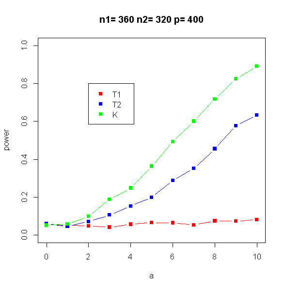
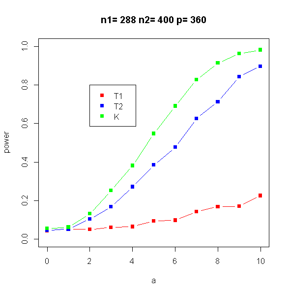
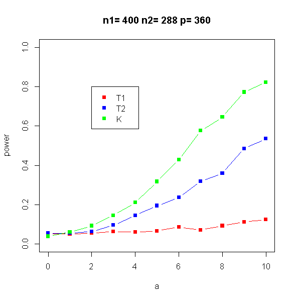
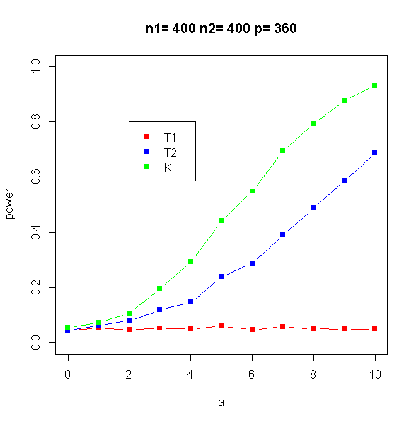
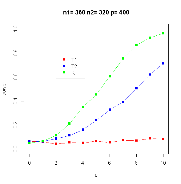
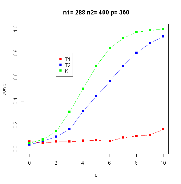
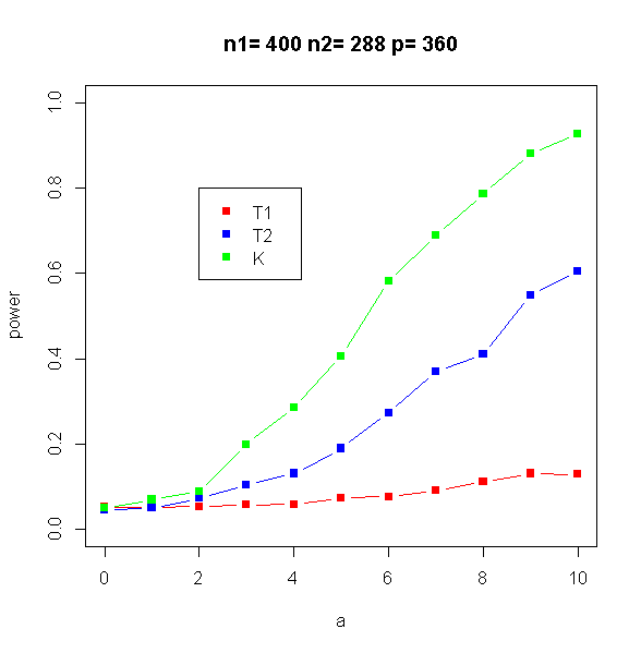
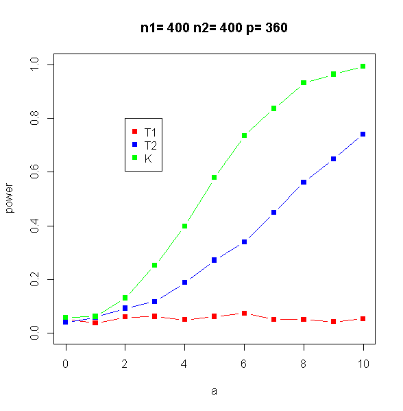
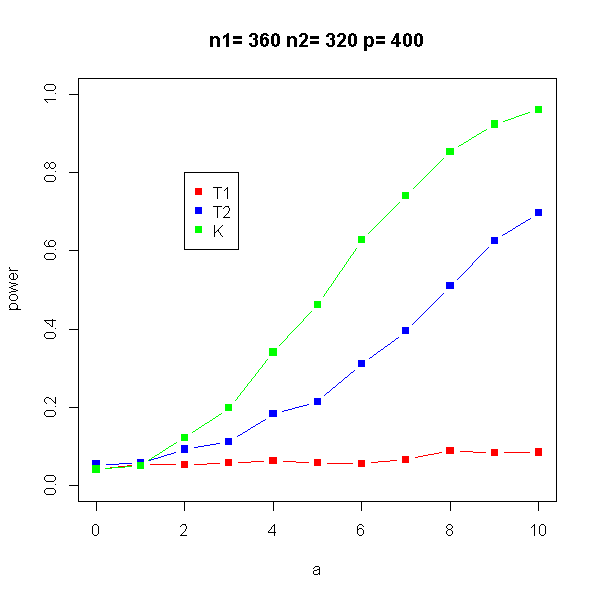
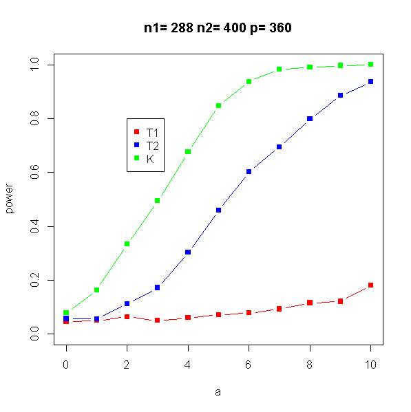
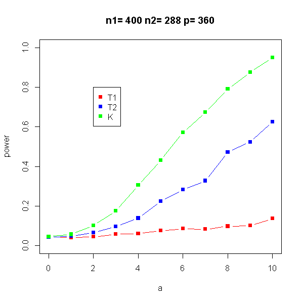
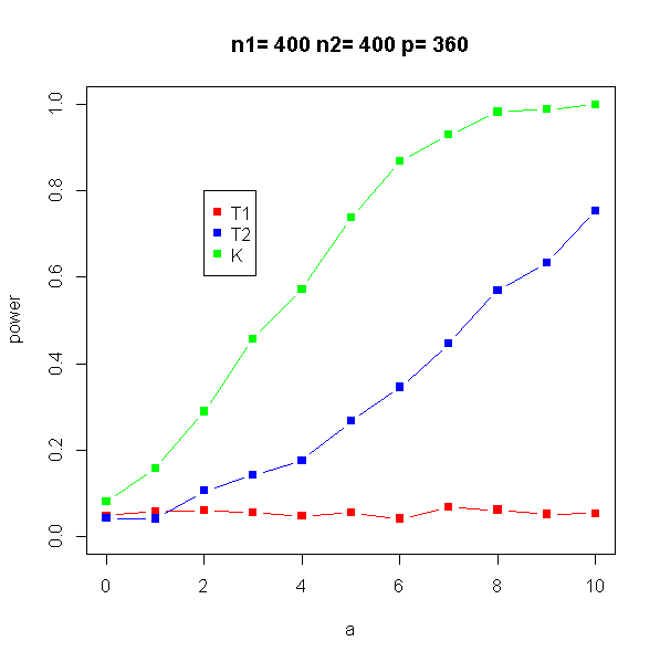
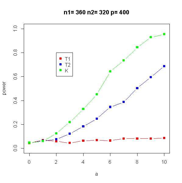
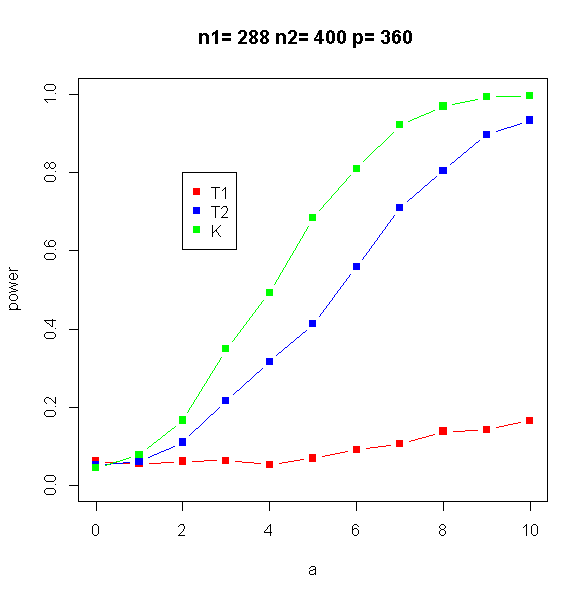
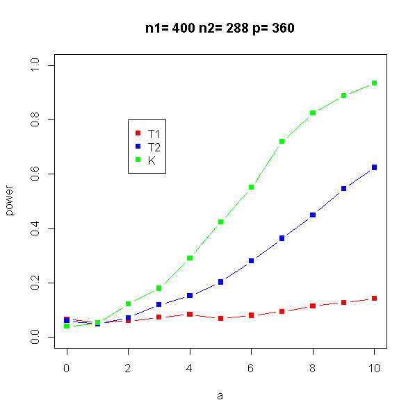
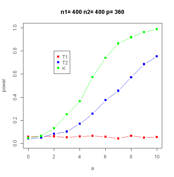
For each case, we consider 161616 choices of (n1,n2,p)subscript𝑛1subscript𝑛2𝑝(n_{1},n_{2},p), four cases are for each (y1>1,y2>1)formulae-sequencesubscript𝑦11subscript𝑦21(y_{1}>1,y_{2}>1), (y1>1,y2<1)formulae-sequencesubscript𝑦11subscript𝑦21(y_{1}>1,y_{2}<1),(y1<1,y2>1)formulae-sequencesubscript𝑦11subscript𝑦21(y_{1}<1,y_{2}>1), (y1<1,y2<1)formulae-sequencesubscript𝑦11subscript𝑦21(y_{1}<1,y_{2}<1). Four choices are considered for a𝑎a, a=0,3,7,10𝑎03710a=0,3,7,10, where a=0𝑎0a=0 is the choice of the null hypothesis. In all cases, we assume that forth moments of 𝐱(1)superscript𝐱1\mathbf{x}^{(1)} and 𝐱(2)superscript𝐱2\mathbf{x}^{(2)} are known. In case 1, Δ1=Δ2=0subscriptΔ1subscriptΔ20\Delta_{1}=\Delta_{2}=0 and in case 2,3, and 4, Δ1=Δ2=1.2subscriptΔ1subscriptΔ21.2\Delta_{1}=\Delta_{2}=-1.2. For each combination, we generate 100010001000 data sets and the powers (the sizes) are evaluated by counting the number of rejected data sets. The results are reported in Tables 1 to 4. In the tables, \mathcal{L} and ~~\tilde{\mathcal{L}} stand for two modified LRTs by Zhang et al. (2019) and 𝒦𝒦\mathcal{K} is our statistic in Theorem 1. Moreover, Figures 2 - 4 display (empirical) powers with respect to different choices of a𝑎a for the Cases 1 - 4. We find that, in all cases considered, the power of 𝒦𝒦\mathcal{K} is higher than both \mathcal{L} and ~~\tilde{\mathcal{L}}.

(i) (n1,n2,p)=(45,40,50)subscript𝑛1subscript𝑛2𝑝454050(n_{1},n_{2},p)=(45,40,50) (n1,n2,p)=(90,80,100)subscript𝑛1subscript𝑛2𝑝9080100(n_{1},n_{2},p)=(90,80,100)
a=0 a=3 a=7 a=10 a=0 a=3 a=7 a=10
\mathcal{L} 0.062 0.056(0.046) 0.058(0.044) 0.070(0.060) 0.050 0.051(0.058) 0.059(0.063) 0.069(0.072)
~~\tilde{\mathcal{L}} 0.061 0.109(0.094) 0.335(0.303) 0.555(0.506) 0.045 0.102(0.110) 0.336(0.350) 0.610(0.625)
𝒦𝒦\mathcal{K} 0.062 0.150(0.141) 0.568(0.535) 0.835(0.821) 0.054 0.129(0.117) 0.603(0.590) 0.869(0.865)
(n1,n2,p)=(180,160,200)subscript𝑛1subscript𝑛2𝑝180160200(n_{1},n_{2},p)=(180,160,200) (n1,n2,p)=(360,320,400)subscript𝑛1subscript𝑛2𝑝360320400(n_{1},n_{2},p)=(360,320,400)
a=0 a=3 a=7 a=10 a=0 a=3 a=7 a=10
\mathcal{L} 0.041 0.043(0.058) 0.063(0.085) 0.070(0.091) 0.056 0.041(0.036) 0.053(0.043) 0.080(0.074)
~~\tilde{\mathcal{L}} 0.047 0.109(0.119) 0.348(0.356) 0.620(0.639) 0.059 0.105(0.092) 0.352(0.330) 0.632(0.606)
𝒦𝒦\mathcal{K} 0.049 0.175(0.182) 0.589(0.597) 0.882(0.886) 0.051 0.188(0.188) 0.601(0.600) 0.891(0.891)
(ii) (n1,n2,p)=(36,50,45)subscript𝑛1subscript𝑛2𝑝365045(n_{1},n_{2},p)=(36,50,45) (n1,n2,p)=(72,100,90)subscript𝑛1subscript𝑛2𝑝7210090(n_{1},n_{2},p)=(72,100,90)
a=0 a=3 a=7 a=10 a=0 a=3 a=7 a=10
\mathcal{L} 0.066 0.071(0.056) 0.110(0.092) 0.227(0.188) 0.056 0.065(0.187) 0.131(0.122) 0.211(0.195)
~~\tilde{\mathcal{L}} 0.049 0.169(0.170) 0.519(0.523) 0.806(0.809) 0.042 0.158(0.187) 0.602(0.639) 0.858(0.874)
𝒦𝒦\mathcal{K} 0.060 0.216(0.187) 0.738(0.718) 0.957(0.952) 0.046 0.224(0.228) 0.807(0.814) 0.974(0.976)
(n1,n2,p)=(144,200,180)subscript𝑛1subscript𝑛2𝑝144200180(n_{1},n_{2},p)=(144,200,180) (n1,n2,p)=(288,400,360)subscript𝑛1subscript𝑛2𝑝288400360(n_{1},n_{2},p)=(288,400,360)
a=0 a=3 a=7 a=10 a=0 a=3 a=7 a=10
\mathcal{L} 0.057 0.055(0.051) 0.130(0.117) 0.209(0.195) 0.043 0.060(0.070) 0.142(0.158) 0.225(0.242)
~~\tilde{\mathcal{L}} 0.065 0.174(0.142) 0.614(0.577) 0.864(0.831) 0.046 0.167(0.175) 0.626(0.635) 0.897(0.901)
𝒦𝒦\mathcal{K} 0.060 0.234(0.209) 0.819(0.795) 0.979(0.975) 0.055 0.251(0.240) 0.827(0.821) 0.982(0.982)
(iii) (n1,n2,p)=(50,36,45)subscript𝑛1subscript𝑛2𝑝503645(n_{1},n_{2},p)=(50,36,45) (n1,n2,p)=(100,72,90)subscript𝑛1subscript𝑛2𝑝1007290(n_{1},n_{2},p)=(100,72,90)
a=0 a=3 a=7 a=10 a=0 a=3 a=7 a=10
\mathcal{L} 0.061 0.056(0.044) 0.095(0.086) 0.116(0.103) 0.061 0.074(0.046) 0.084(0.056) 0.099(0.068)
~~\tilde{\mathcal{L}} 0.060 0.083(0.063) 0.291(0.257) 0.511(0.461) 0.058 0.107(0.097) 0.293(0.276) 0.516(0.498)
𝒦𝒦\mathcal{K} 0.060 0.140(0.123) 0.494(0.473) 0.780(0.758) 0.057 0.153(0.144) 0.505(0.489) 0.822(0.808)
(n1,n2,p)=(200,144,180)subscript𝑛1subscript𝑛2𝑝200144180(n_{1},n_{2},p)=(200,144,180) (n1,n2,p)=(400,288,360)subscript𝑛1subscript𝑛2𝑝400288360(n_{1},n_{2},p)=(400,288,360)
a=0 a=3 a=7 a=10 a=0 a=3 a=7 a=10
\mathcal{L} 0.041 0.051(0.058) 0.083(0.096) 0.142(0.155) 0.053 0.063(0.062) 0.071(0.071) 0.123(0.119)
~~\tilde{\mathcal{L}} 0.042 0.086(0.094) 0.286(0.305) 0.563(0.579) 0.054 0.095(0.093) 0.318(0.312) 0.535(0.525)
𝒦𝒦\mathcal{K} 0.033 0.138(0.176) 0.505(0.565) 0.825(0.849) 0.038 0.145(0.171) 0.576(0.615) 0.822(0.848)
(iv) (n1,n2,p)=(50,50,45)subscript𝑛1subscript𝑛2𝑝505045(n_{1},n_{2},p)=(50,50,45) (n1,n2,p)=(100,100,90)subscript𝑛1subscript𝑛2𝑝10010090(n_{1},n_{2},p)=(100,100,90)
a=0 a=3 a=7 a=10 a=0 a=3 a=7 a=10
\mathcal{L} 0.061 0.059(0.042) 0.047(0.036) 0.061(0.043) 0.063 0.051(0.046) 0.387(0.384) 0.053(0.047)
~~\tilde{\mathcal{L}} 0.059 0.108(0.090) 0.345(0.314) 0.592(0.555) 0.053 0.116(0.113) 0.387(0.384) 0.636(0.632)
𝒦𝒦\mathcal{K} 0.048 0.146(0.154) 0.617(0.624) 0.892(0.896) 0.055 0.202(0.189) 0.666(0.651) 0.907(0.902)
(n1,n2,p)=(200,200,180)subscript𝑛1subscript𝑛2𝑝200200180(n_{1},n_{2},p)=(200,200,180) (n1,n2,p)=(400,400,360)subscript𝑛1subscript𝑛2𝑝400400360(n_{1},n_{2},p)=(400,400,360)
a=0 a=3 a=7 a=10 a=0 a=3 a=7 a=10
\mathcal{L} 0.042 0.060(0.069) 0.059(0.064) 0.047(0.056) 0.044 0.053(0.056) 0.058(0.064) 0.49(0.054)
~~\tilde{\mathcal{L}} 0.049 0.112(0.114) 0.403(0.406) 0.656(0.658) 0.046 0.119(0.130) 0.391(0.408) 0.686(0.700)
𝒦𝒦\mathcal{K} 0.049 0.187(0.187) 0.675(0.678) 0.917(0.917) 0.055 0.195(0.187) 0.694(0.684) 0.931(0.927)
Table 1: Case 1: Empirical sizes and powers. The results are based on the 5% significance level. The power number in small bracket indicates the size corrected power based empirical 95% quantile not asymptotic. (i) indicates the case of y1>1,y2>1formulae-sequencesubscript𝑦11subscript𝑦21y_{1}>1,y_{2}>1, (ii) does y1>1,y2<1formulae-sequencesubscript𝑦11subscript𝑦21y_{1}>1,y_{2}<1, (iii) does y1<1,y2>1formulae-sequencesubscript𝑦11subscript𝑦21y_{1}<1,y_{2}>1, and (iv) does y1<1,y2<1formulae-sequencesubscript𝑦11subscript𝑦21y_{1}<1,y_{2}<1.
(i) (n1,n2,p)=(45,40,50)subscript𝑛1subscript𝑛2𝑝454050(n_{1},n_{2},p)=(45,40,50) (n1,n2,p)=(90,80,100)subscript𝑛1subscript𝑛2𝑝9080100(n_{1},n_{2},p)=(90,80,100)
a=0 a=3 a=7 a=10 a=0 a=3 a=7 a=10
\mathcal{L} 0.060 0.055(0.041) 0.067(0.051) 0.061(0.047) 0.054 0.052(0.047) 0.084(0.075) 0.078(0.072)
~~\tilde{\mathcal{L}} 0.061 0.136(0.120) 0.371(0.328) 0.602(0.572) 0.064 0.129(0.105) 0.396(0.342) 0.666(0.623)
𝒦𝒦\mathcal{K} 0.054 0.203(0.190) 0.700(0.686) 0.917(0.913) 0.052 0.207(0.207) 0.732(0.730) 0.951(0.950)
(n1,n2,p)=(180,160,200)subscript𝑛1subscript𝑛2𝑝180160200(n_{1},n_{2},p)=(180,160,200) (n1,n2,p)=(360,320,400)subscript𝑛1subscript𝑛2𝑝360320400(n_{1},n_{2},p)=(360,320,400)
a=0 a=3 a=7 a=10 a=0 a=3 a=7 a=10
\mathcal{L} 0.045 0.050(0.068) 0.064(0.081) 0.098(0.113) 0.067 0.054(0.040) 0.072(0.056) 0.083(0.062)
~~\tilde{\mathcal{L}} 0.047 0.122(0.130) 0.399(0.410) 0.692(0.712) 0.061 0.114(0.091) 0.392(0.355) 0.711(0.683)
𝒦𝒦\mathcal{K} 0.055 0.199(0.194) 0.742(0.731) 0.953(0.943) 0.050 0.212(0.214) 0.754(0.758) 0.964(0.965)
(ii) (n1,n2,p)=(36,50,45)subscript𝑛1subscript𝑛2𝑝365045(n_{1},n_{2},p)=(36,50,45) (n1,n2,p)=(72,100,90)subscript𝑛1subscript𝑛2𝑝7210090(n_{1},n_{2},p)=(72,100,90)
a=0 a=3 a=7 a=10 a=0 a=3 a=7 a=10
\mathcal{L} 0.060 0.059(0.043) 0.132(0.116) 0.160(0.133) 0.066 0.057(0.044) 0.100(0.078) 0.169(0.129)
~~\tilde{\mathcal{L}} 0.047 0.177(0.184) 0.646(0.660) 0.857(0.858) 0.044 0.168(0.201) 0.681(0.713) 0.919(0.933)
𝒦𝒦\mathcal{K} 0.051 0.283(0.283) 0.890(0.890) 0.991(0.991) 0.048 0.308(0.327) 0.903(0.911) 0.999(0.999)
(n1,n2,p)=(144,200,180)subscript𝑛1subscript𝑛2𝑝144200180(n_{1},n_{2},p)=(144,200,180) (n1,n2,p)=(288,400,360)subscript𝑛1subscript𝑛2𝑝288400360(n_{1},n_{2},p)=(288,400,360)
a=0 a=3 a=7 a=10 a=0 a=3 a=7 a=10
\mathcal{L} 0.056 0.055(0.049) 0.110(0.096) 0.193(0.175) 0.063 0.062(0.059) 0.095(0.087) 0.164(0.148)
~~\tilde{\mathcal{L}} 0.062 0.183(0.176) 0.684(0.665) 0.932(0.919) 0.037 0.165(0.191) 0.692(0.731) 0.937(0.944)
𝒦𝒦\mathcal{K} 0.055 0.321(0.314) 0.914(0.907) 0.998(0.997) 0.050 0.310(0.310) 0.922(0.924) 0.999(0.999)
(iii) (n1,n2,p)=(50,36,45)subscript𝑛1subscript𝑛2𝑝503645(n_{1},n_{2},p)=(50,36,45) (n1,n2,p)=(100,72,90)subscript𝑛1subscript𝑛2𝑝1007290(n_{1},n_{2},p)=(100,72,90)
a=0 a=3 a=7 a=10 a=0 a=3 a=7 a=10
T𝑇T 0.057 0.066(0.057) 0.096(0.088) 0.119(0.104) 0.053 0.053(0.052) 0.104(0.103) 0.129(0.127)
T~~𝑇\tilde{T} 0.057 0.106(0.099) 0.331(0.316) 0.559(0.543) 0.059 0.090(0.079) 0.352(0.314) 0.601(0.552)
𝒦𝒦\mathcal{K} 0.048 0.162(0.176) 0.618(0.640) 0.899(0.909) 0.040 0.181(0.199) 0.667(0.688) 0.927(0.933)
(n1,n2,p)=(200,144,180)subscript𝑛1subscript𝑛2𝑝200144180(n_{1},n_{2},p)=(200,144,180) (n1,n2,p)=(400,288,360)subscript𝑛1subscript𝑛2𝑝400288360(n_{1},n_{2},p)=(400,288,360)
a=0 a=3 a=7 a=10 a=0 a=3 a=7 a=10
\mathcal{L} 0.053 0.066(0.066) 0.089(0.088) 0.129(0.127) 0.052 0.057(0.057) 0.091(0.091) 0.128(0.128)
~~\tilde{\mathcal{L}} 0.052 0.124(0.111) 0.350(0.334) 0.600(0.586) 0.046 0.104(0.109) 0.369(0.380) 0.605(0.618)
𝒦𝒦\mathcal{K} 0.039 0.190(0.214) 0.685(0.718) 0.928(0.941) 0.049 0.199(0.199) 0.689(0.691) 0.926(0.928)
(iv) (n1,n2,p)=(50,50,45)subscript𝑛1subscript𝑛2𝑝505045(n_{1},n_{2},p)=(50,50,45) (n1,n2,p)=(100,100,90)subscript𝑛1subscript𝑛2𝑝10010090(n_{1},n_{2},p)=(100,100,90)
a=0 a=3 a=7 a=10 a=0 a=3 a=7 a=10
\mathcal{L} 0.040 0.051(0.057) 0.049(0.057) 0.050(0.056) 0.048 0.053(0.054) 0.061(0.063) 0.056(0.059)
~~\tilde{\mathcal{L}} 0.046 0.133(0.133) 0.409(0.435) 0.656(0.677) 0.046 0.108(0.113) 0.421(0.434) 0.707(0.713)
𝒦𝒦\mathcal{K} 0.052 0.254(0.250) 0.807(0.806) 0.970(0.970) 0.043 0.222(0.240) 0.814(0.840) 0.981(0.983)
(n1,n2,p)=(200,200,180)subscript𝑛1subscript𝑛2𝑝200200180(n_{1},n_{2},p)=(200,200,180) (n1,n2,p)=(400,400,360)subscript𝑛1subscript𝑛2𝑝400400360(n_{1},n_{2},p)=(400,400,360)
a=0 a=3 a=7 a=10 a=0 a=3 a=7 a=10
\mathcal{L} 0.051 0.052(0.050) 0.055(0.054) 0.050(0.050) 0.050 0.061(0.062) 0.050(0.050) 0.052(0.052)
~~\tilde{\mathcal{L}} 0.050 0.130(0.133) 0.458(0.460) 0.720(0.722) 0.040 0.117(0.127) 0.448(0.462) 0.741(0.754)
𝒦𝒦\mathcal{K} 0.047 0.259(0.268) 0.833(0.846) 0.984(0.986) 0.058 0.252(0.241) 0.836(0.827) 0.994(0.992)
Table 2: Case 2: Empirical sizes and powers. The results are based on the 5% significance level. The power number in small bracket indicates the size corrected power based empirical 95% quantile not asymptotic. (i) indicates the case of y1>1,y2>1formulae-sequencesubscript𝑦11subscript𝑦21y_{1}>1,y_{2}>1, (ii) does y1>1,y2<1formulae-sequencesubscript𝑦11subscript𝑦21y_{1}>1,y_{2}<1, (iii) does y1<1,y2>1formulae-sequencesubscript𝑦11subscript𝑦21y_{1}<1,y_{2}>1, and (iv) does y1<1,y2<1formulae-sequencesubscript𝑦11subscript𝑦21y_{1}<1,y_{2}<1.
(i) (n1,n2,p)=(45,40,50)subscript𝑛1subscript𝑛2𝑝454050(n_{1},n_{2},p)=(45,40,50) (n1,n2,p)=(90,80,100)subscript𝑛1subscript𝑛2𝑝9080100(n_{1},n_{2},p)=(90,80,100)
a=0 a=3 a=7 a=10 a=0 a=3 a=7 a=10
\mathcal{L} 0.055 0.050(0.039) 0.067(0.061) 0.066(0.057) 0.053 0.061(0.059) 0.061(0.055) 0.093(0.088)
~~\tilde{\mathcal{L}} 0.060 0.112(0.102) 0.368(0.354) 0.586(0.570) 0.050 0.124(0.131) 0.372(0.379) 0.645(0.651)
𝒦𝒦\mathcal{K} 0.049 0.185(0.194) 0.717(0.740) 0.915(0.923) 0.054 0.220(0.215) 0.711(0.706) 0.947(0.945)
(n1,n2,p)=(180,160,200)subscript𝑛1subscript𝑛2𝑝180160200(n_{1},n_{2},p)=(180,160,200) (n1,n2,p)=(360,320,400)subscript𝑛1subscript𝑛2𝑝360320400(n_{1},n_{2},p)=(360,320,400)
a=0 a=3 a=7 a=10 a=0 a=3 a=7 a=10
\mathcal{L} 0.035 0.075(0.090) 0.070(0.089) 0.087(0.105) 0.039 0.057(0.072) 0.066(0.076) 0.084(0.096)
~~\tilde{\mathcal{L}} 0.043 0.113(0.122) 0.408(0.423) 0.693(0.705) 0.054 0.111(0.102) 0.394(0.378) 0.697(0.678)
𝒦𝒦\mathcal{K} 0.050 0.186(0.186) 0.738(0.738) 0.955(0.955) 0.041 0.199(0.236) 0.741(0.765) 0.961(0.967)
(ii) (n1,n2,p)=(36,50,45)subscript𝑛1subscript𝑛2𝑝365045(n_{1},n_{2},p)=(36,50,45) (n1,n2,p)=(72,100,90)subscript𝑛1subscript𝑛2𝑝7210090(n_{1},n_{2},p)=(72,100,90)
a=0 a=3 a=7 a=10 a=0 a=3 a=7 a=10
\mathcal{L} 0.070 0.054(0.043) 0.104(0.081) 0.165(0.116) 0.057 0.048(0.043) 0.108(0.099) 0.175(0.163)
~~\tilde{\mathcal{L}} 0.056 0.170(0.159) 0.631(0.619) 0.859(0.853) 0.050 0.185(0.189) 0.654(0.660) 0.921(0.921)
𝒦𝒦\mathcal{K} 0.056 0.280(0.268) 0.880(0.869) 0.979(0.979) 0.052 0.309(0.298) 0.902(0.900) 0.992(0.992)
(n1,n2,p)=(144,200,180)subscript𝑛1subscript𝑛2𝑝144200180(n_{1},n_{2},p)=(144,200,180) (n1,n2,p)=(288,400,360)subscript𝑛1subscript𝑛2𝑝288400360(n_{1},n_{2},p)=(288,400,360)
a=0 a=3 a=7 a=10 a=0 a=3 a=7 a=10
\mathcal{L} 0.054 0.062(0.054) 0.095(0.091) 0.179(0.169) 0.054 0.058(0.055) 0.105(0.103) 0.160(0.156)
~~\tilde{\mathcal{L}} 0.044 0.183(0.192) 0.691(0.700) 0.927(0.928) 0.039 0.182(0.199) 0.669(0.693) 0.934(0.947)
𝒦𝒦\mathcal{K} 0.046 0.295(0.307) 0.902(0.915) 0.999(0.999) 0.047 0.328(0.346) 0.923(0.935) 0.998(0.998)
(iii) (n1,n2,p)=(50,36,45)subscript𝑛1subscript𝑛2𝑝503645(n_{1},n_{2},p)=(50,36,45) (n1,n2,p)=(100,72,90)subscript𝑛1subscript𝑛2𝑝1007290(n_{1},n_{2},p)=(100,72,90)
a=0 a=3 a=7 a=10 a=0 a=3 a=7 a=10
\mathcal{L} 0.060 0.056(0.051) 0.088(0.079) 0.116(0.107) 0.050 0.076(0.076) 0.109(0.110) 0.116(0.116)
~~\tilde{\mathcal{L}} 0.054 0.092(0.074) 0.324(0.301) 0.558(0.541) 0.045 0.112(0.132) 0.354(0.382) 0.592(0.625)
𝒦𝒦\mathcal{K} 0.050 0.155(0.155) 0.645(0.645) 0.903(0.903) 0.044 0.167(0.187) 0.659(0.687) 0.922(0.935)
(n1,n2,p)=(200,144,180)subscript𝑛1subscript𝑛2𝑝200144180(n_{1},n_{2},p)=(200,144,180) (n1,n2,p)=(400,288,360)subscript𝑛1subscript𝑛2𝑝400288360(n_{1},n_{2},p)=(400,288,360)
a=0 a=3 a=7 a=10 a=0 a=3 a=7 a=10
\mathcal{L} 0.061 0.053(0.046) 0.079(0.065) 0.126(0.113) 0.043 0.057(0.060) 0.082(0.091) 0.136(0.147)
~~\tilde{\mathcal{L}} 0.065 0.107(0.085) 0.334(0.299) 0.605(0.565) 0.043 0.096(0.109) 0.327(0.353) 0.626(0.642)
𝒦𝒦\mathcal{K} 0.047 0.176(0.182) 0.676(0.692) 0.923(0.927) 0.045 0.175(0.185) 0.673(0.680) 0.949(0.949)
(iv) (n1,n2,p)=(50,50,45)subscript𝑛1subscript𝑛2𝑝505045(n_{1},n_{2},p)=(50,50,45) (n1,n2,p)=(100,100,90)subscript𝑛1subscript𝑛2𝑝10010090(n_{1},n_{2},p)=(100,100,90)
a=0 a=3 a=7 a=10 a=0 a=3 a=7 a=10
\mathcal{L} 0.065 0.043(0.035) 0.056(0.046) 0.066(0.056) 0.060 0.046(0.042) 0.058(0.053) 0.049(0.046)
~~\tilde{\mathcal{L}} 0.049 0.110(0.112) 0.420(0.425) 0.658(0.665) 0.059 0.135(0.113) 0.419(0.386) 0.700(0.676)
𝒦𝒦\mathcal{K} 0.044 0.223(0.236) 0.780(0.793) 0.967(0.974) 0.050 0.239(0.242) 0.814(0.817) 0.979(0.979)
(n1,n2,p)=(200,200,180)subscript𝑛1subscript𝑛2𝑝200200180(n_{1},n_{2},p)=(200,200,180) (n1,n2,p)(400,400,360)subscript𝑛1subscript𝑛2𝑝400400360(n_{1},n_{2},p)(400,400,360)
a=0 a=3 a=7 a=10 a=0 a=3 a=7 a=10
\mathcal{L} 0.049 0.045(0.046) 0.046(0.046) 0.054(0.057) 0.041 0.057(0.068) 0.047(0.064) 0.061(0.073)
~~\tilde{\mathcal{L}} 0.052 0.117(0.107) 0.419(0.413) 0.744(0.736) 0.041 0.126(0.132) 0.473(0.491) 0.752(0.760)
𝒦𝒦\mathcal{K} 0.050 0.257(0.265) 0.854(0.857) 0.989(0.989) 0.047 0.240(0.250) 0.864(0.868) 0.993(0.993)
Table 3: Case 3: Empirical sizes and powers. The results are based on the 5% significance level. The power number in small bracket indicates the size corrected power based empirical 95% quantile not asymptotic. (i) indicates the case of y1>1,y2>1formulae-sequencesubscript𝑦11subscript𝑦21y_{1}>1,y_{2}>1, (ii) does y1>1,y2<1formulae-sequencesubscript𝑦11subscript𝑦21y_{1}>1,y_{2}<1, (iii) does y1<1,y2>1formulae-sequencesubscript𝑦11subscript𝑦21y_{1}<1,y_{2}>1, and (iv) does y1<1,y2<1formulae-sequencesubscript𝑦11subscript𝑦21y_{1}<1,y_{2}<1.
(i) (n1,n2,p)=(45,40,50)subscript𝑛1subscript𝑛2𝑝454050(n_{1},n_{2},p)=(45,40,50) (n1,n2,p)=(90,80,100)subscript𝑛1subscript𝑛2𝑝9080100(n_{1},n_{2},p)=(90,80,100)
a=0 a=3 a=7 a=10 a=0 a=3 a=7 a=10
\mathcal{L} 0.055 0.069(0.060) 0.074(0.071) 0.083(0.078) 0.058 0.061(0.054) 0.064(0.055) 0.075(0.065)
~~\tilde{\mathcal{L}} 0.057 0.104(0.096) 0.359(0.347) 0.599(0.581) 0.054 0.111(0.109) 0.400(0.396) 0.663(0.659)
𝒦𝒦\mathcal{K} 0.055 0.175(0.166) 0.705(0.686) 0.937(0.933) 0.058 0.179(0.166) 0.743(0.728) 0.956(0.951)
(n1,n2,p)=(180,160,200)subscript𝑛1subscript𝑛2𝑝180160200(n_{1},n_{2},p)=(180,160,200) (n1,n2,p)=(360,320,400)subscript𝑛1subscript𝑛2𝑝360320400(n_{1},n_{2},p)=(360,320,400)
a=0 a=3 a=7 a=10 a=0 a=3 a=7 a=10
\mathcal{L} 0.054 0.061(0.055) 0.058(0.054) 0.091(0.083) 0.042 0.044(0.048) 0.081(0.099) 0.085(0.097)
~~\tilde{\mathcal{L}} 0.059 0.118(0.115) 0.374(0.361) 0.665(0.652) 0.046 0.122(0.142) 0.387(0.423) 0.687(0.722)
𝒦𝒦\mathcal{K} 0.066 0.195(0.150) 0.731(0.690) 0.953(0.943) 0.046 0.219(0.230) 0.735(0.745) 0.954(0.956)
(ii) (n1,n2,p)=(36,50,45)subscript𝑛1subscript𝑛2𝑝365045(n_{1},n_{2},p)=(36,50,45) (n1,n2,p)=(72,100,90)subscript𝑛1subscript𝑛2𝑝7210090(n_{1},n_{2},p)=(72,100,90)
a=0 a=3 a=7 a=10 a=0 a=3 a=7 a=10
\mathcal{L} 0.046 0.058(0.058) 0.119(0.125) 0.174(0.179) 0.064 0.062(0.044) 0.138(0.109) 0.162(0.128)
~~\tilde{\mathcal{L}} 0.037 0.182(0.237) 0.619(0.742) 0.872(0.902) 0.046 0.178(0.189) 0.673(0.685) 0.897(0.904)
𝒦𝒦\mathcal{K} 0.045 0.302(0.315) 0.869(0.874) 0.993(0.993) 0.052 0.295(0.289) 0.899(0.898) 0.995(0.995)
(n1,n2,p)=(144,200,180)subscript𝑛1subscript𝑛2𝑝144200180(n_{1},n_{2},p)=(144,200,180) (n1,n2,p)=(288,400,360)subscript𝑛1subscript𝑛2𝑝288400360(n_{1},n_{2},p)=(288,400,360)
a=0 a=3 a=7 a=10 a=0 a=3 a=7 a=10
\mathcal{L} 0.063 0.048(0.045) 0.108(0.096) 0.163(0.147) 0.061 0.063(0.059) 0.106(0.095) 0.165(0.144)
~~\tilde{\mathcal{L}} 0.044 0.176(0.195) 0.672(0.694) 0.936(0.941) 0.053 0.215(0.211) 0.709(0.701) 0.933(0.931)
𝒦𝒦\mathcal{K} 0.049 0.322(0.324) 0.922(0.922) 0.997(0.997) 0.045 0.349(0.378) 0.921(0.927) 0.996(0.997)
(iii) (n1,n2,p)=(50,36,45)subscript𝑛1subscript𝑛2𝑝503645(n_{1},n_{2},p)=(50,36,45) (n1,n2,p)=(100,72,90)subscript𝑛1subscript𝑛2𝑝1007290(n_{1},n_{2},p)=(100,72,90)
a=0 a=3 a=7 a=10 a=0 a=3 a=7 a=10
\mathcal{L} 0.058 0.073(0.068) 0.085(0.078) 0.125(0.116) 0.051 0.061(0.061) 0.096(0.095) 0.125(0.124)
~~\tilde{\mathcal{L}} 0.061 0.098(0.082) 0.328(0.299) 0.546(0.518) 0.056 0.096(0.088) 0.353(0.330) 0.606(0.579)
𝒦𝒦\mathcal{K} 0.064 0.155(0.143) 0.626(0.599) 0.882(0.860) 0.054 0.166(0.161) 0.666(0.654) 0.914(0.910)
(n1,n2,p)=(200,144,180)subscript𝑛1subscript𝑛2𝑝200144180(n_{1},n_{2},p)=(200,144,180) (n1,n2,p)=(400,288,360)subscript𝑛1subscript𝑛2𝑝400288360(n_{1},n_{2},p)=(400,288,360)
a=0 a=3 a=7 a=10 a=0 a=3 a=7 a=10
\mathcal{L} 0.058 0.078(0.073) 0.087(0.081) 0.114(0.102) 0.066 0.073(0.055) 0.094(0.079) 0.141(0.118)
~~\tilde{\mathcal{L}} 0.046 0.111(0.121) 0.353(0.381) 0.584(0.606) 0.059 0.118(0.103) 0.363(0.324) 0.624(0.578)
𝒦𝒦\mathcal{K} 0.044 0.193(0.213) 0.684(0.701) 0.935(0.939) 0.039 0.179(0.194) 0.720(0.744) 0.934(0.943)
(iv) (n1,n2,p)=(50,50,45)subscript𝑛1subscript𝑛2𝑝505045(n_{1},n_{2},p)=(50,50,45) (n1,n2,p)=(100,100,90)subscript𝑛1subscript𝑛2𝑝10010090(n_{1},n_{2},p)=(100,100,90)
a=0 a=3 a=7 a=10 a=0 a=3 a=7 a=10
\mathcal{L} 0.055 0.046(0.044) 0.058(0.051) 0.068(0.066) 0.064 0.064(0.052) 0.059(0.051) 0.058(0.045)
~~\tilde{\mathcal{L}} 0.059 0.122(0.103) 0.414(0.382) 0.649(0.624) 0.048 0.110(0.114) 0.451(0.456) 0.687(0.694)
𝒦𝒦\mathcal{K} 0.051 0.257(0.256) 0.777(0.774) 0.980(0.979) 0.039 0.234(0.269) 0.826(0.843) 0.983(0.986)
(n1,n2,p)=(200,200,180)subscript𝑛1subscript𝑛2𝑝200200180(n_{1},n_{2},p)=(200,200,180) (n1,n2,p)=(400,400,360)subscript𝑛1subscript𝑛2𝑝400400360(n_{1},n_{2},p)=(400,400,360)
a=0 a=3 a=7 a=10 a=0 a=3 a=7 a=10
\mathcal{L} 0.049 0.053(0.054) 0.045(0.045) 0.057(0.058) 0.058 0.053(0.043) 0.043(0.038) 0.054(0.045)
~~\tilde{\mathcal{L}} 0.050 0.126(0.128) 0.451(0.461) 0.758(0.761) 0.042 0.102(0.116) 0.455(0.477) 0.753(0.769)
𝒦𝒦\mathcal{K} 0.034 0.256(0.313) 0.828(0.874) 0.992(0.995) 0.048 0.251(0.255) 0.864(0.867) 0.988(0.988)
Table 4: Case 4: Empirical sizes and powers. The results are based on the 5% significance level. The power number in small bracket indicates the size corrected power based empirical 95% quantile not asymptotic. (i) indicates the case of y1>1,y2>1formulae-sequencesubscript𝑦11subscript𝑦21y_{1}>1,y_{2}>1, (ii) does y1>1,y2<1formulae-sequencesubscript𝑦11subscript𝑦21y_{1}>1,y_{2}<1, (iii) does y1<1,y2>1formulae-sequencesubscript𝑦11subscript𝑦21y_{1}<1,y_{2}>1, and (iv) does y1<1,y2<1formulae-sequencesubscript𝑦11subscript𝑦21y_{1}<1,y_{2}<1.
Figure 1: Power divergence in Case 1.T1,T2 stand for \mathcal{L} and ~~\tilde{\mathcal{L}} respectively. K𝐾K stands for 𝒦𝒦\mathcal{K}.
Refer to caption Refer to caption
Figure 2: Power divergence in Case 2. T1,T2 stand for \mathcal{L} and ~~\tilde{\mathcal{L}} respectively. K𝐾K stands for 𝒦𝒦\mathcal{K}.
Refer to caption Refer to caption
Figure 3: Power divergence in Case 1.T1,T2 stand for \mathcal{L} and ~~\tilde{\mathcal{L}} respectively. K𝐾K stands for 𝒦𝒦\mathcal{K}.
Refer to caption Refer to caption
Figure 4: Power divergence in Case 1.T1,T2 stand for \mathcal{L} and ~~\tilde{\mathcal{L}} respectively. K𝐾K stands for 𝒦𝒦\mathcal{K}.
Refer to caption Refer to caption

4 Conclusion

In this paper, we suggest an alternative invariant test, named as 𝒦𝒦\mathcal{K}, to two modified LRTs by Zhang et al. (2019) for the equality of two large scale covariance matrices. It is based on the sum of eigenvalues of 𝐁n=n1Sn1(n1Sn1+n2Sn2)1subscript𝐁𝑛subscript𝑛1subscript𝑆subscript𝑛1superscriptsubscript𝑛1subscript𝑆subscript𝑛1subscript𝑛2subscript𝑆subscript𝑛21\mathbf{B}_{n}=n_{1}S_{n_{1}}(n_{1}S_{n_{1}}+n_{2}S_{n_{2}})^{-1}. We find the asymptotic null distribution of 𝒦𝒦\mathcal{K}, when all n1,n2,psubscript𝑛1subscript𝑛2𝑝n_{1},n_{2},p approach \infty at the same rate. The numerical study shows the new invariant test is more powerful than the modified LRTs by Zhang et al. (2019) in all cases we consider. However, we do not claim the proposed 𝒦𝒦\mathcal{K} is the most powerful for the problem because, as we learn from lower dimensional cases, there could be more powerful one than 𝒦𝒦\mathcal{K} for some settings.

Acknowledgement

This research is supported by National Research Foundation of Korea (Grant Number: NRF-2017R1A2B 2012264).

Appendix: Proof of Theorem 1

We will use the Cauchy’s residue theorem and Lemma A.1. in Zhang et al. (2019).

Lemma 2 (Zhang et al. 2019, Lemma A.1).

In addition to the Moments Assumption and the Dimensions Assumption, we further assume that:

  • (1)

    as min{p,n1,n2}𝑝subscript𝑛1subscript𝑛2\min\{p,n_{1},n_{2}\}\rightarrow\infty, y1γ1(0,1)(1,)subscript𝑦1subscript𝛾1011y_{1}\rightarrow\gamma_{1}\in(0,1)\cup(1,\infty), y2γ2(0,1)(1,)subscript𝑦2subscript𝛾2011y_{2}\rightarrow\gamma_{2}\in(0,1)\cup(1,\infty), and αnα>0subscript𝛼𝑛𝛼0\alpha_{n}\rightarrow\alpha>0.

  • (2)

    let f1,,fksubscript𝑓1subscript𝑓𝑘f_{1},\ldots,f_{k} be the analytic functions on an open region containing the interval [al,ar]subscript𝑎𝑙subscript𝑎𝑟[a_{l},a_{r}], where al=v1(1γ1)2subscript𝑎𝑙superscript𝑣1superscript1subscript𝛾12a_{l}=v^{-1}(1-\sqrt{\gamma_{1}})^{2}, ar=1αv1(1γ2)2subscript𝑎𝑟1𝛼superscript𝑣1superscript1subscript𝛾22a_{r}=1-\alpha v^{-1}(1-\sqrt{\gamma_{2}})^{2}, and v𝑣v is defined as v=(1+γ1γ2)(1γ1γ2γ1+γ2)2𝑣1subscript𝛾1subscript𝛾2superscript1subscript𝛾1subscript𝛾2subscript𝛾1subscript𝛾22v=\left(1+\frac{\gamma_{1}}{\gamma_{2}}\right)\left(1-\sqrt{\frac{\gamma_{1}\gamma_{2}}{\gamma_{1}+\gamma_{2}}}\right)^{2}.

Then, as min{p,n1,n2}𝑝subscript𝑛1subscript𝑛2\min\{p,n_{1},n_{2}\}\rightarrow\infty, the random vector

(fi𝑑Gn)i=1,,ksubscriptsubscript𝑓𝑖differential-dsubscript𝐺𝑛𝑖1𝑘\left(\int f_{i}dG_{n}\right)_{i=1,\ldots,k}

converges weakly to a Gaussian vector (Gf1,,Gfk)subscript𝐺subscript𝑓1subscript𝐺subscript𝑓𝑘\left(G_{f_{1}},\ldots,G_{f_{k}}\right) with mean functions

𝔼Gfi=14πifi(zα+z)dlog((1γ2)m32(z)+2m3(z)+1γ1(1+m3(z))2)𝔼subscript𝐺subscript𝑓𝑖14𝜋𝑖contour-integralsubscript𝑓𝑖𝑧𝛼𝑧𝑑1subscript𝛾2superscriptsubscript𝑚32𝑧2subscript𝑚3𝑧1subscript𝛾1superscript1subscript𝑚3𝑧2\displaystyle\mathbb{E}G_{f_{i}}=\frac{1}{4\pi i}\oint f_{i}\left(\frac{z}{\alpha+z}\right)d\log\left(\frac{(1-\gamma_{2})m_{3}^{2}(z)+2m_{3}(z)+1-\gamma_{1}}{\left(1+m_{3}(z)\right)^{2}}\right)
+Δ12πiγ1fi(zα+z)(1+m3(z))3𝑑m3(z)subscriptΔ12𝜋𝑖contour-integralsubscript𝛾1subscript𝑓𝑖𝑧𝛼𝑧superscript1subscript𝑚3𝑧3differential-dsubscript𝑚3𝑧\displaystyle\quad+\frac{\Delta_{1}}{2\pi i}\oint\gamma_{1}f_{i}\left(\frac{z}{\alpha+z}\right)(1+m_{3}(z))^{-3}dm_{3}(z)
+Δ24πifi(zα+z)(1γ2m32(z)(1+m3(z))2)dlog(1γ2m32(z)(1+m3(z))2)subscriptΔ24𝜋𝑖contour-integralsubscript𝑓𝑖𝑧𝛼𝑧1subscript𝛾2superscriptsubscript𝑚32𝑧superscript1subscript𝑚3𝑧2𝑑1subscript𝛾2superscriptsubscript𝑚32𝑧superscript1subscript𝑚3𝑧2\displaystyle\quad+\frac{\Delta_{2}}{4\pi i}\oint f_{i}\left(\frac{z}{\alpha+z}\right)\left(1-\frac{\gamma_{2}m_{3}^{2}(z)}{\left(1+m_{3}(z)\right)^{2}}\right)d\log\left(1-\frac{\gamma_{2}m_{3}^{2}(z)}{\left(1+m_{3}(z)\right)^{2}}\right) (7)

and covariance functions

Cov(Gfi,Gfj)=12π2fi(z1α+z1)fj(z2α+z2)dm3(z1)dm3(z2)(m3(z1)m3(z2))2Covsubscript𝐺subscript𝑓𝑖subscript𝐺subscript𝑓𝑗12superscript𝜋2contour-integralcontour-integralsubscript𝑓𝑖subscript𝑧1𝛼subscript𝑧1subscript𝑓𝑗subscript𝑧2𝛼subscript𝑧2𝑑subscript𝑚3subscript𝑧1𝑑subscript𝑚3subscript𝑧2superscriptsubscript𝑚3subscript𝑧1subscript𝑚3subscript𝑧22\displaystyle{\rm Cov}(G_{f_{i}},G_{f_{j}})=-\frac{1}{2\pi^{2}}\oint\oint\frac{f_{i}\left(\frac{z_{1}}{\alpha+z_{1}}\right)f_{j}\left(\frac{z_{2}}{\alpha+z_{2}}\right)dm_{3}(z_{1})dm_{3}(z_{2})}{(m_{3}(z_{1})-m_{3}(z_{2}))^{2}}
γ1Δ1+γ2Δ24π2fi(z1α+z1)fj(z2α+z2)dm3(z1)dm3(z2)(m3(z1)+1)2(m3(z2)+1)2subscript𝛾1subscriptΔ1subscript𝛾2subscriptΔ24superscript𝜋2contour-integralcontour-integralsubscript𝑓𝑖subscript𝑧1𝛼subscript𝑧1subscript𝑓𝑗subscript𝑧2𝛼subscript𝑧2𝑑subscript𝑚3subscript𝑧1𝑑subscript𝑚3subscript𝑧2superscriptsubscript𝑚3subscript𝑧112superscriptsubscript𝑚3subscript𝑧212\displaystyle\quad-\frac{\gamma_{1}\Delta_{1}+\gamma_{2}\Delta_{2}}{4\pi^{2}}\oint\oint\frac{f_{i}\left(\frac{z_{1}}{\alpha+z_{1}}\right)f_{j}\left(\frac{z_{2}}{\alpha+z_{2}}\right)dm_{3}(z_{1})dm_{3}(z_{2})}{(m_{3}(z_{1})+1)^{2}(m_{3}(z_{2})+1)^{2}} (8)

where

m0(z)subscript𝑚0𝑧\displaystyle m_{0}(z) =\displaystyle= (1+γ1)(1z)αz(1γ2)2z(1z)(γ1(1z)+αzγ2)1subscript𝛾11𝑧𝛼𝑧1subscript𝛾22𝑧1𝑧subscript𝛾11𝑧𝛼𝑧subscript𝛾2\displaystyle\frac{(1+\gamma_{1})(1-z)-\alpha z(1-\gamma_{2})}{2z(1-z)(\gamma_{1}(1-z)+\alpha z\gamma_{2})}
+((1γ1)(1z)+αz(1γ2))24αz(1z)2z(1z)(γ1(1z)+αzγ2)1z,superscript1subscript𝛾11𝑧𝛼𝑧1subscript𝛾224𝛼𝑧1𝑧2𝑧1𝑧subscript𝛾11𝑧𝛼𝑧subscript𝛾21𝑧\displaystyle\quad+\frac{\sqrt{\left((1-\gamma_{1})(1-z)+\alpha z(1-\gamma_{2})\right)^{2}-4\alpha z(1-z)}}{2z(1-z)(\gamma_{1}(1-z)+\alpha z\gamma_{2})}-\frac{1}{z},
m1(z)subscript𝑚1𝑧\displaystyle m_{1}(z) =\displaystyle= α(α+z)2m0(zα+z)1α+z,𝛼superscript𝛼𝑧2subscript𝑚0𝑧𝛼𝑧1𝛼𝑧\displaystyle\frac{\alpha}{(\alpha+z)^{2}}m_{0}\left(\frac{z}{\alpha+z}\right)-\frac{1}{\alpha+z},
m2(z)subscript𝑚2𝑧\displaystyle m_{2}(z) =\displaystyle= 1γ1z+γ1m1(z),1subscript𝛾1𝑧subscript𝛾1subscript𝑚1𝑧\displaystyle-\frac{1-\gamma_{1}}{z}+\gamma_{1}m_{1}(z),
mmpγ2(z)superscriptsubscript𝑚𝑚𝑝subscript𝛾2𝑧\displaystyle m_{mp}^{\gamma_{2}}(z) =\displaystyle= 1γ2z+(z1γ2)24γ22γ2z,1subscript𝛾2𝑧superscript𝑧1subscript𝛾224subscript𝛾22subscript𝛾2𝑧\displaystyle\frac{1-\gamma_{2}-z+\sqrt{(z-1-\gamma_{2})^{2}-4\gamma_{2}}}{2\gamma_{2}z},
m3(z)subscript𝑚3𝑧\displaystyle m_{3}(z) =\displaystyle= γ2mmpγ2(m2(z))+1γ2m2(z).subscript𝛾2superscriptsubscript𝑚𝑚𝑝subscript𝛾2subscript𝑚2𝑧1subscript𝛾2subscript𝑚2𝑧\displaystyle\gamma_{2}m_{mp}^{\gamma_{2}}(-m_{2}(z))+\frac{1-\gamma_{2}}{m_{2}(z)}.

All of the above contour integrals can be evaluated on any contour enclosing the interval [αcl1cl,αcr1cr]𝛼subscript𝑐𝑙1subscript𝑐𝑙𝛼subscript𝑐𝑟1subscript𝑐𝑟\left[\frac{\alpha c_{l}}{1-c_{l}},\frac{\alpha c_{r}}{1-c_{r}}\right].

Proof of Theorem 1.

The proof of Theorem 1 consists of three parts: the proof of the limit part lnsubscript𝑙𝑛l_{n}, the proof of the limit part μnsubscript𝜇𝑛\mu_{n}, and the proof of the limit part σn2superscriptsubscript𝜎𝑛2\sigma_{n}^{2}.

Proof of the limit part lnsubscript𝑙𝑛l_{n}.

We need to calculate the following integrals:

xlxrx(αn+1)(xrx)(xxl)2πy1x(1x)𝑑xandsuperscriptsubscriptsubscript𝑥𝑙subscript𝑥𝑟𝑥subscript𝛼𝑛1subscript𝑥𝑟𝑥𝑥subscript𝑥𝑙2𝜋subscript𝑦1𝑥1𝑥differential-d𝑥and\displaystyle\int_{x_{l}}^{x_{r}}x\frac{(\alpha_{n}+1)\sqrt{(x_{r}-x)(x-x_{l})}}{2\pi y_{1}x(1-x)}dx\quad\mbox{and} (9)
xlxr(1x)(αn+1)(xrx)(xxl)2πy1x(1x)𝑑x.superscriptsubscriptsubscript𝑥𝑙subscript𝑥𝑟1𝑥subscript𝛼𝑛1subscript𝑥𝑟𝑥𝑥subscript𝑥𝑙2𝜋subscript𝑦1𝑥1𝑥differential-d𝑥\displaystyle\int_{x_{l}}^{x_{r}}(1-x)\frac{(\alpha_{n}+1)\sqrt{(x_{r}-x)(x-x_{l})}}{2\pi y_{1}x(1-x)}dx. (10)

To get these values, we choose a transformation

x=y2|y1+hξ|2(y1+y2)2.𝑥subscript𝑦2superscriptsubscript𝑦1𝜉2superscriptsubscript𝑦1subscript𝑦22x=\frac{y_{2}\left|y_{1}+h\xi\right|^{2}}{(y_{1}+y_{2})^{2}}. (11)

We can see that the integral (9) is rewritten as

(9)=y2h2i4π(y1+y2)|ξ|=1(ξ21)2ξ3|y2hξ|2𝑑ξ.italic-(9italic-)subscript𝑦2superscript2𝑖4𝜋subscript𝑦1subscript𝑦2subscriptcontour-integral𝜉1superscriptsuperscript𝜉212superscript𝜉3superscriptsubscript𝑦2𝜉2differential-d𝜉\eqref{eq:l_n1}=\frac{y_{2}h^{2}i}{4\pi(y_{1}+y_{2})}\oint_{|\xi|=1}\frac{(\xi^{2}-1)^{2}}{\xi^{3}|y_{2}-h\xi|^{2}}d\xi.

The singularities of the integrand are 0, y2hsubscript𝑦2\frac{y_{2}}{h}, and hy2subscript𝑦2\frac{h}{y_{2}}. If y2>1subscript𝑦21y_{2}>1, then y22h2=(y1+y2)(y21)>0superscriptsubscript𝑦22superscript2subscript𝑦1subscript𝑦2subscript𝑦210y_{2}^{2}-h^{2}=(y_{1}+y_{2})(y_{2}-1)>0, so y2>hsubscript𝑦2y_{2}>h. It implies that if y2>1subscript𝑦21y_{2}>1, y2hsubscript𝑦2\frac{y_{2}}{h} is not a pole, thus 00 and hy2subscript𝑦2\frac{h}{y_{2}} are only poles of the integrand. On the other hand, if y2<1subscript𝑦21y_{2}<1, then y2<hsubscript𝑦2y_{2}<h and thus 0 and y2hsubscript𝑦2\frac{y_{2}}{h} are only poles of the integrand. First, we assume y2>1subscript𝑦21y_{2}>1. Using Cauchy’s residue theorem, we get the following result:

(9)italic-(9italic-)\displaystyle\eqref{eq:l_n1} =\displaystyle= y2h2i4π(y1+y2)2πi[ddξ(ξ21)2(y2hξ)(y2ξh)|ξ=0+(ξ21)2y2ξ2(y2hξ)|ξ=hy2]subscript𝑦2superscript2𝑖4𝜋subscript𝑦1subscript𝑦22𝜋𝑖delimited-[]evaluated-at𝑑𝑑𝜉superscriptsuperscript𝜉212subscript𝑦2𝜉subscript𝑦2𝜉𝜉0evaluated-atsuperscriptsuperscript𝜉212subscript𝑦2superscript𝜉2subscript𝑦2𝜉𝜉subscript𝑦2\displaystyle\frac{y_{2}h^{2}i}{4\pi(y_{1}+y_{2})}2\pi i\left[\left.\frac{d}{d\xi}\frac{(\xi^{2}-1)^{2}}{(y_{2}-h\xi)(y_{2}\xi-h)}\right|_{\xi=0}+\left.\frac{(\xi^{2}-1)^{2}}{y_{2}\xi^{2}(y_{2}-h\xi)}\right|_{\xi=\frac{h}{y_{2}}}\right]
=\displaystyle= h2y2(y1+y2).superscript2subscript𝑦2subscript𝑦1subscript𝑦2\displaystyle\frac{h^{2}}{y_{2}(y_{1}+y_{2})}.

Next, we assume y2<1subscript𝑦21y_{2}<1. Using Cauchy’s residue theorem again, we can calculate the integral (9) as

(9)italic-(9italic-)\displaystyle\eqref{eq:l_n1} =\displaystyle= y2h2i4π(y1+y2)[ddξ(ξ21)2(y2hξ)(y2ξh)|ξ=0(ξ21)2hξ2(y2ξh)|ξ=y2h]subscript𝑦2superscript2𝑖4𝜋subscript𝑦1subscript𝑦2delimited-[]evaluated-at𝑑𝑑𝜉superscriptsuperscript𝜉212subscript𝑦2𝜉subscript𝑦2𝜉𝜉0evaluated-atsuperscriptsuperscript𝜉212superscript𝜉2subscript𝑦2𝜉𝜉subscript𝑦2\displaystyle\frac{y_{2}h^{2}i}{4\pi(y_{1}+y_{2})}\left[\left.\frac{d}{d\xi}\frac{(\xi^{2}-1)^{2}}{(y_{2}-h\xi)(y_{2}\xi-h)}\right|_{\xi=0}-\left.\frac{(\xi^{2}-1)^{2}}{h\xi^{2}(y_{2}\xi-h)}\right|_{\xi=\frac{y_{2}}{h}}\right]
=\displaystyle= y2y1+y2.subscript𝑦2subscript𝑦1subscript𝑦2\displaystyle\frac{y_{2}}{y_{1}+y_{2}}.

Now, we consider the integral (10). Using the transformation (11), the integral (10) is rewritten as

(10)=y1h2i4π(y1+y2)|ξ|=1(ξ21)2ξ3|y1+hξ|2𝑑ξ.italic-(10italic-)subscript𝑦1superscript2𝑖4𝜋subscript𝑦1subscript𝑦2subscriptcontour-integral𝜉1superscriptsuperscript𝜉212superscript𝜉3superscriptsubscript𝑦1𝜉2differential-d𝜉\eqref{eq:l_n2}=\frac{y_{1}h^{2}i}{4\pi(y_{1}+y_{2})}\oint_{|\xi|=1}\frac{(\xi^{2}-1)^{2}}{\xi^{3}|y_{1}+h\xi|^{2}}d\xi.

We note that the singularities of the integrand of (10) are 0, y1hsubscript𝑦1-\frac{y_{1}}{h}, and hy1subscript𝑦1-\frac{h}{y_{1}} of which absolute values are greater than or less than 1 depending only on the size of y1subscript𝑦1y_{1}. It implies that the value of (10) does not depend on the size of y2subscript𝑦2y_{2}. Since xlxr(αn+1)(xrx)(xxl)2πy1x(1x)𝑑x=h2y1y2superscriptsubscriptsubscript𝑥𝑙subscript𝑥𝑟subscript𝛼𝑛1subscript𝑥𝑟𝑥𝑥subscript𝑥𝑙2𝜋subscript𝑦1𝑥1𝑥differential-d𝑥superscript2subscript𝑦1subscript𝑦2\int_{x_{l}}^{x_{r}}\frac{(\alpha_{n}+1)\sqrt{(x_{r}-x)(x-x_{l})}}{2\pi y_{1}x(1-x)}dx=\frac{h^{2}}{y_{1}y_{2}} for y1,y2>1subscript𝑦1subscript𝑦21y_{1},y_{2}>1, we can easily calculate the value of (10) when y1>1subscript𝑦11y_{1}>1 as

(10)=h2y1y2h2y2(y1+y2)=h2y1(y1+y2).italic-(10italic-)superscript2subscript𝑦1subscript𝑦2superscript2subscript𝑦2subscript𝑦1subscript𝑦2superscript2subscript𝑦1subscript𝑦1subscript𝑦2\eqref{eq:l_n2}=\frac{h^{2}}{y_{1}y_{2}}-\frac{h^{2}}{y_{2}(y_{1}+y_{2})}=\frac{h^{2}}{y_{1}(y_{1}+y_{2})}.

Similarly, if y1<1subscript𝑦11y_{1}<1, then

(10)=1y2y1+y2=y1y1+y2.italic-(10italic-)1subscript𝑦2subscript𝑦1subscript𝑦2subscript𝑦1subscript𝑦1subscript𝑦2\eqref{eq:l_n2}=1-\frac{y_{2}}{y_{1}+y_{2}}=\frac{y_{1}}{y_{1}+y_{2}}.

Here, we used the fact that xlxr(αn+1)(xrx)(xxl)2πy1x(1x)𝑑x=1superscriptsubscriptsubscript𝑥𝑙subscript𝑥𝑟subscript𝛼𝑛1subscript𝑥𝑟𝑥𝑥subscript𝑥𝑙2𝜋subscript𝑦1𝑥1𝑥differential-d𝑥1\int_{x_{l}}^{x_{r}}\frac{(\alpha_{n}+1)\sqrt{(x_{r}-x)(x-x_{l})}}{2\pi y_{1}x(1-x)}dx=1 for y1,y2<1subscript𝑦1subscript𝑦21y_{1},y_{2}<1. ∎

Proof of the limit part μnsubscript𝜇𝑛\mu_{n}.

According to Lemma 5.1 in Bai et al. (2015), m3subscript𝑚3m_{3} satisfies the equation

z=m3(m3+1y1)(1y2)(m3+11y2).𝑧subscript𝑚3subscript𝑚31subscript𝑦11subscript𝑦2subscript𝑚311subscript𝑦2z=-\frac{m_{3}(m_{3}+1-y_{1})}{(1-y_{2})(m_{3}+\frac{1}{1-y_{2}})}.

As in the proof of the limit part μ~nsubscript~𝜇𝑛\tilde{\mu}_{n} of Theorem 2.5 in Zhang et al. (2019), by making an integral conversion

z=(1+hrξ)(1+hrξ)(1y2)2,𝑧1𝑟𝜉1𝑟𝜉superscript1subscript𝑦22z=\frac{(1+hr\xi)(1+\frac{h}{r\xi})}{(1-y_{2})^{2}},

where r𝑟r is a number greter than but close to 1, m3subscript𝑚3m_{3} satisfies

(1+hrξ)(1+hrξ)(1y2)2=m3(m3+1y1)(1y2)m3+1.1𝑟𝜉1𝑟𝜉superscript1subscript𝑦22subscript𝑚3subscript𝑚31subscript𝑦11subscript𝑦2subscript𝑚31\frac{(1+hr\xi)(1+\frac{h}{r\xi})}{(1-y_{2})^{2}}=-\frac{m_{3}(m_{3}+1-y_{1})}{(1-y_{2})m_{3}+1}.

By the above equation, we can obtain m3=1+hrξ1y2subscript𝑚31𝑟𝜉1subscript𝑦2m_{3}=-\frac{1+\frac{h}{r\xi}}{1-y_{2}} or m3=1+hrξ1y2subscript𝑚31𝑟𝜉1subscript𝑦2m_{3}=-\frac{1+hr\xi}{1-y_{2}}. When z𝑧z runs in the positive direction around the contour enclosing the interval [αcl1cl,αcr1cr]𝛼subscript𝑐𝑙1subscript𝑐𝑙𝛼subscript𝑐𝑟1subscript𝑐𝑟[\frac{\alpha c_{l}}{1-c_{l}},\frac{\alpha c_{r}}{1-c_{r}}], m3subscript𝑚3m_{3} runs in the opposite direction. Thus, by substituting

m3(z)={1+hrξ1y2if y2>1,1+hrξ1y2if y2<1,subscript𝑚3𝑧cases1𝑟𝜉1subscript𝑦2if subscript𝑦21missing-subexpressionmissing-subexpression1𝑟𝜉1subscript𝑦2if subscript𝑦21m_{3}(z)=\left\{\begin{array}[]{l l}\displaystyle-\frac{1+\frac{h}{r\xi}}{1-y_{2}}&\quad\mbox{if }y_{2}>1,\\ \\ \displaystyle-\frac{1+hr\xi}{1-y_{2}}&\quad\mbox{if }y_{2}<1,\end{array}\right.

where r𝑟r is a real number greater than but close to 1, we observe the followings :

zα+z=(ξ+1hr)(ξ+hr)(ξ+y2hr)(ξ+hy2r),𝑧𝛼𝑧𝜉1𝑟𝜉𝑟𝜉subscript𝑦2𝑟𝜉subscript𝑦2𝑟\displaystyle\frac{z}{\alpha+z}=\frac{\left(\xi+\frac{1}{hr}\right)\left(\xi+\frac{h}{r}\right)}{\left(\xi+\frac{y_{2}}{hr}\right)\left(\xi+\frac{h}{y_{2}r}\right)},
dlog((1y2)m32(z)+2m3(z)+1y1(1+m3(z))2)𝑑1subscript𝑦2superscriptsubscript𝑚32𝑧2subscript𝑚3𝑧1subscript𝑦1superscript1subscript𝑚3𝑧2\displaystyle d\log\left(\frac{(1-y_{2})m_{3}^{2}(z)+2m_{3}(z)+1-y_{1}}{\left(1+m_{3}(z)\right)^{2}}\right)
={(1ξ1r+1ξ+1r2ξ+hy2r)dξif y2>1,(1ξ1r+1ξ+1r2ξ+y2hr)dξif y2<1,absentcases1𝜉1𝑟1𝜉1𝑟2𝜉subscript𝑦2𝑟𝑑𝜉if subscript𝑦21missing-subexpressionmissing-subexpression1𝜉1𝑟1𝜉1𝑟2𝜉subscript𝑦2𝑟𝑑𝜉if subscript𝑦21\displaystyle\qquad\qquad=\left\{\begin{array}[]{l l}\left(\frac{1}{\xi-\frac{1}{r}}+\frac{1}{\xi+\frac{1}{r}}-\frac{2}{\xi+\frac{h}{y_{2}r}}\right)d\xi&\mbox{if }y_{2}>1,\\ \\ \left(\frac{1}{\xi-\frac{1}{r}}+\frac{1}{\xi+\frac{1}{r}}-\frac{2}{\xi+\frac{y_{2}}{hr}}\right)d\xi&\mbox{if }y_{2}<1,\end{array}\right. (15)
(1+m3(z))3dm3(z)={(1y2)2hy231(ξ+y2hr)3dξif y2>1,(1y2)2h21(ξ+y2hr)3dξif y2<1,superscript1subscript𝑚3𝑧3𝑑subscript𝑚3𝑧casessuperscript1subscript𝑦22superscriptsubscript𝑦231superscript𝜉subscript𝑦2𝑟3𝑑𝜉if subscript𝑦21missing-subexpressionmissing-subexpressionsuperscript1subscript𝑦22superscript21superscript𝜉subscript𝑦2𝑟3𝑑𝜉if subscript𝑦21\displaystyle(1+m_{3}(z))^{-3}dm_{3}(z)=\left\{\begin{array}[]{l l}\frac{(1-y_{2})^{2}h}{y_{2}^{3}}\frac{1}{(\xi+\frac{y_{2}}{hr})^{3}}d\xi&\mbox{if }y_{2}>1,\\ \\ \frac{(1-y_{2})^{2}}{h^{2}}\frac{1}{(\xi+\frac{y_{2}}{hr})^{3}}d\xi&\mbox{if }y_{2}<1,\end{array}\right. (19)
(1y2m32(z)(1+m3(z))2)dlog(1y2m32(z)(1+m3(z))2)1subscript𝑦2superscriptsubscript𝑚32𝑧superscript1subscript𝑚3𝑧2𝑑1subscript𝑦2superscriptsubscript𝑚32𝑧superscript1subscript𝑚3𝑧2\displaystyle\left(1-\frac{y_{2}m_{3}^{2}(z)}{(1+m_{3}(z))^{2}}\right)d\log\left(1-\frac{y_{2}m_{3}^{2}(z)}{(1+m_{3}(z))^{2}}\right)
={(y21)(ξ2h2y2r2)y2(ξ+hy2r)2(2ξξ2h2y2r22ξ+hy2r)dξif y2>1,(1y2)(ξ2y2h2r2)(ξ+y2hr)2(2ξξ2y2h2r22ξ+y2hr)dξif y2<1.absentcasessubscript𝑦21superscript𝜉2superscript2subscript𝑦2superscript𝑟2subscript𝑦2superscript𝜉subscript𝑦2𝑟22𝜉superscript𝜉2superscript2subscript𝑦2superscript𝑟22𝜉subscript𝑦2𝑟𝑑𝜉if subscript𝑦21missing-subexpressionmissing-subexpression1subscript𝑦2superscript𝜉2subscript𝑦2superscript2superscript𝑟2superscript𝜉subscript𝑦2𝑟22𝜉superscript𝜉2subscript𝑦2superscript2superscript𝑟22𝜉subscript𝑦2𝑟𝑑𝜉if subscript𝑦21\displaystyle\qquad\qquad=\left\{\begin{array}[]{l l}\frac{(y_{2}-1)\left(\xi^{2}-\frac{h^{2}}{y_{2}r^{2}}\right)}{y_{2}\left(\xi+\frac{h}{y_{2}r}\right)^{2}}\left(\frac{2\xi}{\xi^{2}-\frac{h^{2}}{y_{2}r^{2}}}-\frac{2}{\xi+\frac{h}{y_{2}r}}\right)d\xi&\mbox{if }y_{2}>1,\\ \\ \frac{(1-y_{2})\left(\xi^{2}-\frac{y_{2}}{h^{2}r^{2}}\right)}{\left(\xi+\frac{y_{2}}{hr}\right)^{2}}\left(\frac{2\xi}{\xi^{2}-\frac{y_{2}}{h^{2}r^{2}}}-\frac{2}{\xi+\frac{y_{2}}{hr}}\right)d\xi&\mbox{if }y_{2}<1.\end{array}\right. (23)

First, we assume y2>1subscript𝑦21y_{2}>1. Then, the mean part is same with

𝔼Gf1=limr114πi|ξ|=1zα+z(1ξ1r+1ξ+1r2ξ+hy2r)𝑑ξ𝔼subscript𝐺subscript𝑓1subscript𝑟114𝜋𝑖subscriptcontour-integral𝜉1𝑧𝛼𝑧1𝜉1𝑟1𝜉1𝑟2𝜉subscript𝑦2𝑟differential-d𝜉\displaystyle\mathbb{E}G_{f_{1}}=\lim_{r\downarrow 1}\frac{1}{4\pi i}\oint_{|\xi|=1}\frac{z}{\alpha+z}\left(\frac{1}{\xi-\frac{1}{r}}+\frac{1}{\xi+\frac{1}{r}}-\frac{2}{\xi+\frac{h}{y_{2}r}}\right)d\xi (24)
+limr1y1Δ12πi|ξ|=1zα+z(1y2)2hy23ξ(ξ+hy2r)3𝑑ξsubscript𝑟1subscript𝑦1subscriptΔ12𝜋𝑖subscriptcontour-integral𝜉1𝑧𝛼𝑧superscript1subscript𝑦22superscriptsubscript𝑦23𝜉superscript𝜉subscript𝑦2𝑟3differential-d𝜉\displaystyle\quad+\lim_{r\downarrow 1}\frac{-y_{1}\Delta_{1}}{2\pi i}\oint_{|\xi|=1}\frac{z}{\alpha+z}\frac{(1-y_{2})^{2}h}{y_{2}^{3}}\frac{\xi}{(\xi+\frac{h}{y_{2}r})^{3}}d\xi (25)
+limr1Δ24πi|ξ|=1zα+z(y21)(ξ2h2y2r2)y2(ξ+hy2r)2(2ξξ2h2y2r22ξ+hy2r)𝑑ξ.subscript𝑟1subscriptΔ24𝜋𝑖subscriptcontour-integral𝜉1𝑧𝛼𝑧subscript𝑦21superscript𝜉2superscript2subscript𝑦2superscript𝑟2subscript𝑦2superscript𝜉subscript𝑦2𝑟22𝜉superscript𝜉2superscript2subscript𝑦2superscript𝑟22𝜉subscript𝑦2𝑟differential-d𝜉\displaystyle\quad+\lim_{r\downarrow 1}\frac{\Delta_{2}}{4\pi i}\oint_{|\xi|=1}\frac{z}{\alpha+z}\frac{(y_{2}-1)(\xi^{2}-\frac{h^{2}}{y_{2}r^{2}})}{y_{2}(\xi+\frac{h}{y_{2}r})^{2}}\left(\frac{2\xi}{\xi^{2}-\frac{h^{2}}{y_{2}r^{2}}}-\frac{2}{\xi+\frac{h}{y_{2}r}}\right)d\xi. (26)

In (24), the poles are ±1rplus-or-minus1𝑟\pm\frac{1}{r} and hy2rsubscript𝑦2𝑟-\frac{h}{y_{2}r}. Hence, (24) can be calculated as

(24)=limr114πi|ξ|=1(ξ+1hr)(ξ+hr)(ξ+y2hr)(ξ+hy2r)(1ξ1r+1ξ+1r2ξ+hy2r)𝑑ξitalic-(24italic-)subscript𝑟114𝜋𝑖subscriptcontour-integral𝜉1𝜉1𝑟𝜉𝑟𝜉subscript𝑦2𝑟𝜉subscript𝑦2𝑟1𝜉1𝑟1𝜉1𝑟2𝜉subscript𝑦2𝑟differential-d𝜉\displaystyle\eqref{eq:mean_1}=\lim_{r\downarrow 1}\frac{1}{4\pi i}\oint_{|\xi|=1}\frac{\left(\xi+\frac{1}{hr}\right)\left(\xi+\frac{h}{r}\right)}{\left(\xi+\frac{y_{2}}{hr}\right)\left(\xi+\frac{h}{y_{2}r}\right)}\left(\frac{1}{\xi-\frac{1}{r}}+\frac{1}{\xi+\frac{1}{r}}-\frac{2}{\xi+\frac{h}{y_{2}r}}\right)d\xi
=12[(ξ+1hr)(ξ+hr)(ξ+y2hr)(ξ+hy2r)|ξ=1r+(ξ+1hr)(ξ+hr)(ξ+y2hr)(ξ+hy2r)|ξ=1r\displaystyle=\frac{1}{2}\left[\left.\frac{\left(\xi+\frac{1}{hr}\right)\left(\xi+\frac{h}{r}\right)}{\left(\xi+\frac{y_{2}}{hr}\right)\left(\xi+\frac{h}{y_{2}r}\right)}\right|_{\xi=\frac{1}{r}}+\left.\frac{\left(\xi+\frac{1}{hr}\right)\left(\xi+\frac{h}{r}\right)}{\left(\xi+\frac{y_{2}}{hr}\right)\left(\xi+\frac{h}{y_{2}r}\right)}\right|_{\xi=-\frac{1}{r}}\right.
+(ξ+1hr)(ξ+hr)(ξ+y2hr)(1ξ1r+1ξ+1r)|ξ=hy2r2ddξ(ξ+1hr)(ξ+hr)(ξ+y2hr)|ξ=hy2r]\displaystyle\quad\left.+\left.\frac{\left(\xi+\frac{1}{hr}\right)\left(\xi+\frac{h}{r}\right)}{\left(\xi+\frac{y_{2}}{hr}\right)}\left(\frac{1}{\xi-\frac{1}{r}}+\frac{1}{\xi+\frac{1}{r}}\right)\right|_{\xi=-\frac{h}{y_{2}r}}-2\left.\frac{d}{d\xi}\frac{\left(\xi+\frac{1}{hr}\right)\left(\xi+\frac{h}{r}\right)}{\left(\xi+\frac{y_{2}}{hr}\right)}\right|_{\xi=-\frac{h}{y_{2}r}}\right]
=0.absent0\displaystyle=0.

Here, we used the relations (y12h2)=(y1+y2)(y11)superscriptsubscript𝑦12superscript2subscript𝑦1subscript𝑦2subscript𝑦11(y_{1}^{2}-h^{2})=(y_{1}+y_{2})(y_{1}-1) and (y1h2)=y2(y11)subscript𝑦1superscript2subscript𝑦2subscript𝑦11(y_{1}-h^{2})=y_{2}(y_{1}-1). Similarly, (25) and (26) can be calculated as follows :

(25)italic-(25italic-)\displaystyle\eqref{eq:mean_2} =\displaystyle= limr1y1(1y2)2hΔ12πiy23|ξ|=1ξ(ξ+1hr)(ξ+hr)(ξ+y2hr)(ξ+hy2r)4𝑑ξsubscript𝑟1subscript𝑦1superscript1subscript𝑦22subscriptΔ12𝜋𝑖superscriptsubscript𝑦23subscriptcontour-integral𝜉1𝜉𝜉1𝑟𝜉𝑟𝜉subscript𝑦2𝑟superscript𝜉subscript𝑦2𝑟4differential-d𝜉\displaystyle\lim_{r\downarrow 1}\frac{-y_{1}(1-y_{2})^{2}h\Delta_{1}}{2\pi iy_{2}^{3}}\oint_{|\xi|=1}\frac{\xi\left(\xi+\frac{1}{hr}\right)\left(\xi+\frac{h}{r}\right)}{\left(\xi+\frac{y_{2}}{hr}\right)\left(\xi+\frac{h}{y_{2}r}\right)^{4}}d\xi
=\displaystyle= limr1y1(1y2)2hΔ1y2316d3dξ3ξ(ξ+1hr)(ξ+hr)(ξ+y2hr)|ξ=hy2revaluated-atsubscript𝑟1subscript𝑦1superscript1subscript𝑦22subscriptΔ1superscriptsubscript𝑦2316superscript𝑑3𝑑superscript𝜉3𝜉𝜉1𝑟𝜉𝑟𝜉subscript𝑦2𝑟𝜉subscript𝑦2𝑟\displaystyle\lim_{r\downarrow 1}\frac{-y_{1}(1-y_{2})^{2}h\Delta_{1}}{y_{2}^{3}}\left.\frac{1}{6}\frac{d^{3}}{d\xi^{3}}\frac{\xi\left(\xi+\frac{1}{hr}\right)\left(\xi+\frac{h}{r}\right)}{\left(\xi+\frac{y_{2}}{hr}\right)}\right|_{\xi=-\frac{h}{y_{2}r}}
=\displaystyle= Δ1h2y12y22(y1+y2)4,subscriptΔ1superscript2superscriptsubscript𝑦12superscriptsubscript𝑦22superscriptsubscript𝑦1subscript𝑦24\displaystyle-\frac{\Delta_{1}h^{2}y_{1}^{2}y_{2}^{2}}{(y_{1}+y_{2})^{4}},
(26)italic-(26italic-)\displaystyle\eqref{eq:mean_3} =\displaystyle= limr1Δ24πi|ξ|=1(ξ+1hr)(ξ+hr)(ξ+y2hr)(ξ+hy2r)(y21)(ξ2h2y2r2)y2(ξ+hy2r)2(2ξξ2h2y2r22ξ+hy2r)𝑑ξsubscript𝑟1subscriptΔ24𝜋𝑖subscriptcontour-integral𝜉1𝜉1𝑟𝜉𝑟𝜉subscript𝑦2𝑟𝜉subscript𝑦2𝑟subscript𝑦21superscript𝜉2superscript2subscript𝑦2superscript𝑟2subscript𝑦2superscript𝜉subscript𝑦2𝑟22𝜉superscript𝜉2superscript2subscript𝑦2superscript𝑟22𝜉subscript𝑦2𝑟differential-d𝜉\displaystyle\lim_{r\downarrow 1}\frac{\Delta_{2}}{4\pi i}\oint_{|\xi|=1}\frac{\left(\xi+\frac{1}{hr}\right)\left(\xi+\frac{h}{r}\right)}{\left(\xi+\frac{y_{2}}{hr}\right)\left(\xi+\frac{h}{y_{2}r}\right)}\frac{(y_{2}-1)(\xi^{2}-\frac{h^{2}}{y_{2}r^{2}})}{y_{2}(\xi+\frac{h}{y_{2}r})^{2}}\left(\frac{2\xi}{\xi^{2}-\frac{h^{2}}{y_{2}r^{2}}}-\frac{2}{\xi+\frac{h}{y_{2}r}}\right)d\xi
=\displaystyle= limr1Δ2(y21)2πiy2[|ξ|=1ξ(ξ+1hr)(ξ+hr)(ξ+y2hr)(ξ+hy2r)3dξ\displaystyle\lim_{r\downarrow 1}\frac{\Delta_{2}(y_{2}-1)}{2\pi iy_{2}}\left[\oint_{|\xi|=1}\frac{\xi\left(\xi+\frac{1}{hr}\right)\left(\xi+\frac{h}{r}\right)}{\left(\xi+\frac{y_{2}}{hr}\right)\left(\xi+\frac{h}{y_{2}r}\right)^{3}}d\xi\right.
+|ξ|=1(ξ+1hr)(ξ+hr)(ξ2h2y2r2)(ξ+y2hr)(ξ+hy2r)4dξ]\displaystyle\qquad\qquad\qquad\qquad\qquad\qquad\left.+\oint_{|\xi|=1}\frac{\left(\xi+\frac{1}{hr}\right)\left(\xi+\frac{h}{r}\right)\left(\xi^{2}-\frac{h^{2}}{y_{2}r^{2}}\right)}{\left(\xi+\frac{y_{2}}{hr}\right)\left(\xi+\frac{h}{y_{2}r}\right)^{4}}d\xi\right]
=\displaystyle= limr1Δ2(y21)y2[12d2dξ2ξ(ξ+1hr)(ξ+hr)(ξ+y2hr)\displaystyle\lim_{r\downarrow 1}\frac{\Delta_{2}(y_{2}-1)}{y_{2}}\left[\frac{1}{2}\frac{d^{2}}{d\xi^{2}}\frac{\xi\left(\xi+\frac{1}{hr}\right)\left(\xi+\frac{h}{r}\right)}{\left(\xi+\frac{y_{2}}{hr}\right)}\right.
+16d3dξ3(ξ+1hr)(ξ+hr)(ξ2h2y2r2)(ξ+y2hr)]ξ=hy2r\displaystyle\qquad\qquad\qquad\qquad\qquad\qquad\qquad\left.+\frac{1}{6}\frac{d^{3}}{d\xi^{3}}\frac{\left(\xi+\frac{1}{hr}\right)\left(\xi+\frac{h}{r}\right)\left(\xi^{2}-\frac{h^{2}}{y_{2}r^{2}}\right)}{\left(\xi+\frac{y_{2}}{hr}\right)}\right]_{\xi=-\frac{h}{y_{2}r}}
=\displaystyle= Δ2h2y12y22(y1+y2)4.subscriptΔ2superscript2superscriptsubscript𝑦12superscriptsubscript𝑦22superscriptsubscript𝑦1subscript𝑦24\displaystyle\frac{\Delta_{2}h^{2}y_{1}^{2}y_{2}^{2}}{(y_{1}+y_{2})^{4}}.

Therefore, when y2>1subscript𝑦21y_{2}>1,

𝔼Gf1=Δ1h2y12y22(y1+y2)4+Δ2h2y12y22(y1+y2)4.𝔼subscript𝐺subscript𝑓1subscriptΔ1superscript2superscriptsubscript𝑦12superscriptsubscript𝑦22superscriptsubscript𝑦1subscript𝑦24subscriptΔ2superscript2superscriptsubscript𝑦12superscriptsubscript𝑦22superscriptsubscript𝑦1subscript𝑦24\mathbb{E}G_{f_{1}}=-\frac{\Delta_{1}h^{2}y_{1}^{2}y_{2}^{2}}{(y_{1}+y_{2})^{4}}+\frac{\Delta_{2}h^{2}y_{1}^{2}y_{2}^{2}}{(y_{1}+y_{2})^{4}}.

For the case in which y2<1subscript𝑦21y_{2}<1, we observe

𝔼Gf1=limr114πi|ξ|=1zα+z(1ξ1r+1ξ+1r2ξ+y2hr)𝑑ξ𝔼subscript𝐺subscript𝑓1subscript𝑟114𝜋𝑖subscriptcontour-integral𝜉1𝑧𝛼𝑧1𝜉1𝑟1𝜉1𝑟2𝜉subscript𝑦2𝑟differential-d𝜉\displaystyle\mathbb{E}G_{f_{1}}=\lim_{r\downarrow 1}\frac{1}{4\pi i}\oint_{|\xi|=1}\frac{z}{\alpha+z}\left(\frac{1}{\xi-\frac{1}{r}}+\frac{1}{\xi+\frac{1}{r}}-\frac{2}{\xi+\frac{y_{2}}{hr}}\right)d\xi (27)
+limr1y1Δ12πi|ξ|=1zα+z(1y2)2h2ξ(ξ+y2hr)3𝑑ξsubscript𝑟1subscript𝑦1subscriptΔ12𝜋𝑖subscriptcontour-integral𝜉1𝑧𝛼𝑧superscript1subscript𝑦22superscript2𝜉superscript𝜉subscript𝑦2𝑟3differential-d𝜉\displaystyle\quad+\lim_{r\downarrow 1}\frac{-y_{1}\Delta_{1}}{2\pi i}\oint_{|\xi|=1}\frac{z}{\alpha+z}\frac{(1-y_{2})^{2}}{h^{2}}\frac{\xi}{(\xi+\frac{y_{2}}{hr})^{3}}d\xi (28)
+limr1Δ24πi|ξ|=1zα+z(1y2)(ξ2y2h2r2)(ξ+y2hr)2(2ξξ2y2h2r22ξ+y2hr)𝑑ξ.subscript𝑟1subscriptΔ24𝜋𝑖subscriptcontour-integral𝜉1𝑧𝛼𝑧1subscript𝑦2superscript𝜉2subscript𝑦2superscript2superscript𝑟2superscript𝜉subscript𝑦2𝑟22𝜉superscript𝜉2subscript𝑦2superscript2superscript𝑟22𝜉subscript𝑦2𝑟differential-d𝜉\displaystyle\quad+\lim_{r\downarrow 1}\frac{\Delta_{2}}{4\pi i}\oint_{|\xi|=1}\frac{z}{\alpha+z}\frac{(1-y_{2})(\xi^{2}-\frac{y_{2}}{h^{2}r^{2}})}{(\xi+\frac{y_{2}}{hr})^{2}}\left(\frac{2\xi}{\xi^{2}-\frac{y_{2}}{h^{2}r^{2}}}-\frac{2}{\xi+\frac{y_{2}}{hr}}\right)d\xi. (29)

Through a simple calculation similar to the above, we can show

𝔼Gf1=Δ1h2y12y22(y1+y2)4+Δ2h2y12y22(y1+y2)4.𝔼subscript𝐺subscript𝑓1subscriptΔ1superscript2superscriptsubscript𝑦12superscriptsubscript𝑦22superscriptsubscript𝑦1subscript𝑦24subscriptΔ2superscript2superscriptsubscript𝑦12superscriptsubscript𝑦22superscriptsubscript𝑦1subscript𝑦24\mathbb{E}G_{f_{1}}=-\frac{\Delta_{1}h^{2}y_{1}^{2}y_{2}^{2}}{(y_{1}+y_{2})^{4}}+\frac{\Delta_{2}h^{2}y_{1}^{2}y_{2}^{2}}{(y_{1}+y_{2})^{4}}.

when y2<1subscript𝑦21y_{2}<1. Therefore, it holds that

μn=Δ1h2y12y22(y1+y2)4+Δ2h2y12y22(y1+y2)4.subscript𝜇𝑛subscriptΔ1superscript2superscriptsubscript𝑦12superscriptsubscript𝑦22superscriptsubscript𝑦1subscript𝑦24subscriptΔ2superscript2superscriptsubscript𝑦12superscriptsubscript𝑦22superscriptsubscript𝑦1subscript𝑦24\mu_{n}=-\frac{\Delta_{1}h^{2}y_{1}^{2}y_{2}^{2}}{(y_{1}+y_{2})^{4}}+\frac{\Delta_{2}h^{2}y_{1}^{2}y_{2}^{2}}{(y_{1}+y_{2})^{4}}.

Finally, we note that according to the equation (5) the expectation of the LSS of 𝒫2subscript𝒫2\mathcal{P}_{2} is the opposite sign of that of 𝒫1subscript𝒫1\mathcal{P}_{1}. ∎

Proof of the limit part σn2superscriptsubscript𝜎𝑛2\sigma_{n}^{2}.

We need to calculate the following integral :

Var(Gf1)=12π2z1α+z1z2α+z2dm3(z1)dm3(z2)(m3(z1)m3(z2))2Varsubscript𝐺subscript𝑓112superscript𝜋2contour-integralcontour-integralsubscript𝑧1𝛼subscript𝑧1subscript𝑧2𝛼subscript𝑧2𝑑subscript𝑚3subscript𝑧1𝑑subscript𝑚3subscript𝑧2superscriptsubscript𝑚3subscript𝑧1subscript𝑚3subscript𝑧22\displaystyle{\rm Var}(G_{f_{1}})=-\frac{1}{2\pi^{2}}\oint\oint\frac{z_{1}}{\alpha+z_{1}}\frac{z_{2}}{\alpha+z_{2}}\frac{dm_{3}(z_{1})dm_{3}(z_{2})}{(m_{3}(z_{1})-m_{3}(z_{2}))^{2}}
γ1Δ1+γ2Δ24π2z1α+z1z2α+z2dm3(z1)dm3(z2)(m3(z1)+1)2(m3(z2)+1)2subscript𝛾1subscriptΔ1subscript𝛾2subscriptΔ24superscript𝜋2contour-integralcontour-integralsubscript𝑧1𝛼subscript𝑧1subscript𝑧2𝛼subscript𝑧2𝑑subscript𝑚3subscript𝑧1𝑑subscript𝑚3subscript𝑧2superscriptsubscript𝑚3subscript𝑧112superscriptsubscript𝑚3subscript𝑧212\displaystyle\quad-\frac{\gamma_{1}\Delta_{1}+\gamma_{2}\Delta_{2}}{4\pi^{2}}\oint\oint\frac{z_{1}}{\alpha+z_{1}}\frac{z_{2}}{\alpha+z_{2}}\frac{dm_{3}(z_{1})dm_{3}(z_{2})}{(m_{3}(z_{1})+1)^{2}(m_{3}(z_{2})+1)^{2}} (30)

First, we consider the case in which y2>1subscript𝑦21y_{2}>1. In this case, we observe

dm3(z1)dm3(z2)(m3(z1)m3(z2))2𝑑subscript𝑚3subscript𝑧1𝑑subscript𝑚3subscript𝑧2superscriptsubscript𝑚3subscript𝑧1subscript𝑚3subscript𝑧22\displaystyle\frac{dm_{3}(z_{1})dm_{3}(z_{2})}{(m_{3}(z_{1})-m_{3}(z_{2}))^{2}} =\displaystyle= (1y2)2(hr1ξ1hr2ξ2)2hdξ1(1y2)r1ξ12hdξ2(1y2)r2ξ22=r1r2dξ1dξ2(r1ξ1r2ξ2)2,superscript1subscript𝑦22superscriptsubscript𝑟1subscript𝜉1subscript𝑟2subscript𝜉22𝑑subscript𝜉11subscript𝑦2subscript𝑟1superscriptsubscript𝜉12𝑑subscript𝜉21subscript𝑦2subscript𝑟2superscriptsubscript𝜉22subscript𝑟1subscript𝑟2𝑑subscript𝜉1𝑑subscript𝜉2superscriptsubscript𝑟1subscript𝜉1subscript𝑟2subscript𝜉22\displaystyle\frac{(1-y_{2})^{2}}{(\frac{h}{r_{1}\xi_{1}}-\frac{h}{r_{2}\xi_{2}})^{2}}\frac{hd\xi_{1}}{(1-y_{2})r_{1}\xi_{1}^{2}}\frac{hd\xi_{2}}{(1-y_{2})r_{2}\xi_{2}^{2}}=\frac{r_{1}r_{2}d\xi_{1}d\xi_{2}}{(r_{1}\xi_{1}-r_{2}\xi_{2})^{2}},
dm3(z1)(m3(z1)+1)2𝑑subscript𝑚3subscript𝑧1superscriptsubscript𝑚3subscript𝑧112\displaystyle\frac{dm_{3}(z_{1})}{(m_{3}(z_{1})+1)^{2}} =\displaystyle= (1y2)2(y2+hr1ξ1)2hdξ1(1y2)r1ξ12=(1y2)r1hdξ1(y2r1ξ1+h)2,superscript1subscript𝑦22superscriptsubscript𝑦2subscript𝑟1subscript𝜉12𝑑subscript𝜉11subscript𝑦2subscript𝑟1superscriptsubscript𝜉121subscript𝑦2subscript𝑟1𝑑subscript𝜉1superscriptsubscript𝑦2subscript𝑟1subscript𝜉12\displaystyle\frac{(1-y_{2})^{2}}{(y_{2}+\frac{h}{r_{1}\xi_{1}})^{2}}\frac{hd\xi_{1}}{(1-y_{2})r_{1}\xi_{1}^{2}}=\frac{(1-y_{2})r_{1}hd\xi_{1}}{(y_{2}r_{1}\xi_{1}+h)^{2}},
dm3(z2)(m3(z2)+1)2𝑑subscript𝑚3subscript𝑧2superscriptsubscript𝑚3subscript𝑧212\displaystyle\frac{dm_{3}(z_{2})}{(m_{3}(z_{2})+1)^{2}} =\displaystyle= (1y2)2(y2+hr2ξ2)2hdξ2(1y2)r2ξ22=(1y2)r2hdξ2(y2r2ξ2+h)2.superscript1subscript𝑦22superscriptsubscript𝑦2subscript𝑟2subscript𝜉22𝑑subscript𝜉21subscript𝑦2subscript𝑟2superscriptsubscript𝜉221subscript𝑦2subscript𝑟2𝑑subscript𝜉2superscriptsubscript𝑦2subscript𝑟2subscript𝜉22\displaystyle\frac{(1-y_{2})^{2}}{(y_{2}+\frac{h}{r_{2}\xi_{2}})^{2}}\frac{hd\xi_{2}}{(1-y_{2})r_{2}\xi_{2}^{2}}=\frac{(1-y_{2})r_{2}hd\xi_{2}}{(y_{2}r_{2}\xi_{2}+h)^{2}}.

Assuming r1<r2subscript𝑟1subscript𝑟2r_{1}<r_{2} without loss of generality, the first term of (30) can calculated as follows.

12π2z1α+z1z2α+z2dm3(z1)dm3(z2)(m3(z1)m3(z2))212superscript𝜋2contour-integralcontour-integralsubscript𝑧1𝛼subscript𝑧1subscript𝑧2𝛼subscript𝑧2𝑑subscript𝑚3subscript𝑧1𝑑subscript𝑚3subscript𝑧2superscriptsubscript𝑚3subscript𝑧1subscript𝑚3subscript𝑧22\displaystyle-\frac{1}{2\pi^{2}}\oint\oint\frac{z_{1}}{\alpha+z_{1}}\frac{z_{2}}{\alpha+z_{2}}\frac{dm_{3}(z_{1})dm_{3}(z_{2})}{(m_{3}(z_{1})-m_{3}(z_{2}))^{2}}
=limr21limr1112π2|ξ2|=1(ξ2+1hr2)(ξ2+hr2)(ξ2+y2hr2)(ξ2+hy2r2)absentsubscriptsubscript𝑟21subscriptsubscript𝑟1112superscript𝜋2subscriptcontour-integralsubscript𝜉21subscript𝜉21subscript𝑟2subscript𝜉2subscript𝑟2subscript𝜉2subscript𝑦2subscript𝑟2subscript𝜉2subscript𝑦2subscript𝑟2\displaystyle\quad=\lim_{r_{2}\downarrow 1}\lim_{r_{1}\downarrow 1}-\frac{1}{2\pi^{2}}\oint_{\left|\xi_{2}\right|=1}\frac{\left(\xi_{2}+\frac{1}{hr_{2}}\right)\left(\xi_{2}+\frac{h}{r_{2}}\right)}{\left(\xi_{2}+\frac{y_{2}}{hr_{2}}\right)\left(\xi_{2}+\frac{h}{y_{2}r_{2}}\right)}
[|ξ1|=1(ξ1+1hr1)(ξ1+hr1)(ξ1+y2hr1)(ξ1+hy2r1)r1r2(r1ξ1r2ξ2)2𝑑ξ1]dξ2delimited-[]subscriptcontour-integralsubscript𝜉11subscript𝜉11subscript𝑟1subscript𝜉1subscript𝑟1subscript𝜉1subscript𝑦2subscript𝑟1subscript𝜉1subscript𝑦2subscript𝑟1subscript𝑟1subscript𝑟2superscriptsubscript𝑟1subscript𝜉1subscript𝑟2subscript𝜉22differential-dsubscript𝜉1𝑑subscript𝜉2\displaystyle\qquad\qquad\left[\oint_{\left|\xi_{1}\right|=1}\frac{\left(\xi_{1}+\frac{1}{hr_{1}}\right)\left(\xi_{1}+\frac{h}{r_{1}}\right)}{\left(\xi_{1}+\frac{y_{2}}{hr_{1}}\right)\left(\xi_{1}+\frac{h}{y_{2}r_{1}}\right)}\frac{r_{1}r_{2}}{(r_{1}\xi_{1}-r_{2}\xi_{2})^{2}}d\xi_{1}\right]d\xi_{2}
=limr211πi|ξ2|=1(ξ2+1hr2)(ξ2+hr2)(ξ2+y2hr2)(ξ2+hy2r2)h(y2h2)(y21)y2r2(y22h2)(ξ2+hy2r2)𝑑ξ2absentsubscriptsubscript𝑟211𝜋𝑖subscriptcontour-integralsubscript𝜉21subscript𝜉21subscript𝑟2subscript𝜉2subscript𝑟2subscript𝜉2subscript𝑦2subscript𝑟2subscript𝜉2subscript𝑦2subscript𝑟2subscript𝑦2superscript2subscript𝑦21subscript𝑦2subscript𝑟2superscriptsubscript𝑦22superscript2subscript𝜉2subscript𝑦2subscript𝑟2differential-dsubscript𝜉2\displaystyle\quad=\lim_{r_{2}\downarrow 1}\frac{1}{\pi i}\oint_{\left|\xi_{2}\right|=1}\frac{\left(\xi_{2}+\frac{1}{hr_{2}}\right)\left(\xi_{2}+\frac{h}{r_{2}}\right)}{\left(\xi_{2}+\frac{y_{2}}{hr_{2}}\right)\left(\xi_{2}+\frac{h}{y_{2}r_{2}}\right)}\frac{h(y_{2}-h^{2})(y_{2}-1)}{y_{2}r_{2}(y_{2}^{2}-h^{2})\left(\xi_{2}+\frac{h}{y_{2}r_{2}}\right)}d\xi_{2}
=2h2y12y22(y1+y2)4absent2superscript2superscriptsubscript𝑦12superscriptsubscript𝑦22superscriptsubscript𝑦1subscript𝑦24\displaystyle\quad=\frac{2h^{2}y_{1}^{2}y_{2}^{2}}{(y_{1}+y_{2})^{4}}

The second term of (30) can be expressed as

y1Δ1+y2Δ24π2z1α+z1z2α+z2dm3(z1)dm3(z2)(m3(z1)+1)2(m3(z2)+1)2subscript𝑦1subscriptΔ1subscript𝑦2subscriptΔ24superscript𝜋2contour-integralcontour-integralsubscript𝑧1𝛼subscript𝑧1subscript𝑧2𝛼subscript𝑧2𝑑subscript𝑚3subscript𝑧1𝑑subscript𝑚3subscript𝑧2superscriptsubscript𝑚3subscript𝑧112superscriptsubscript𝑚3subscript𝑧212\displaystyle-\frac{y_{1}\Delta_{1}+y_{2}\Delta_{2}}{4\pi^{2}}\oint\oint\frac{z_{1}}{\alpha+z_{1}}\frac{z_{2}}{\alpha+z_{2}}\frac{dm_{3}(z_{1})dm_{3}(z_{2})}{(m_{3}(z_{1})+1)^{2}(m_{3}(z_{2})+1)^{2}}
=y1Δ1+y2Δ24π2z1α+z1dm3(z1)(m3(z1)+1)2×z2α+z2dm3(z2)(m3(z2)+1)2absentsubscript𝑦1subscriptΔ1subscript𝑦2subscriptΔ24superscript𝜋2contour-integralsubscript𝑧1𝛼subscript𝑧1𝑑subscript𝑚3subscript𝑧1superscriptsubscript𝑚3subscript𝑧112contour-integralsubscript𝑧2𝛼subscript𝑧2𝑑subscript𝑚3subscript𝑧2superscriptsubscript𝑚3subscript𝑧212\displaystyle\quad=-\frac{y_{1}\Delta_{1}+y_{2}\Delta_{2}}{4\pi^{2}}\oint\frac{z_{1}}{\alpha+z_{1}}\frac{dm_{3}(z_{1})}{(m_{3}(z_{1})+1)^{2}}\times\oint\frac{z_{2}}{\alpha+z_{2}}\frac{dm_{3}(z_{2})}{(m_{3}(z_{2})+1)^{2}}
=(y1Δ1+y2Δ2)(h2y1y2(y1+y2)3)2=(y1Δ1+y2Δ2)h4y12y22(y1+y2)6absentsubscript𝑦1subscriptΔ1subscript𝑦2subscriptΔ2superscriptsuperscript2subscript𝑦1subscript𝑦2superscriptsubscript𝑦1subscript𝑦232subscript𝑦1subscriptΔ1subscript𝑦2subscriptΔ2superscript4superscriptsubscript𝑦12superscriptsubscript𝑦22superscriptsubscript𝑦1subscript𝑦26\displaystyle\quad=(y_{1}\Delta_{1}+y_{2}\Delta_{2})\left(-\frac{h^{2}y_{1}y_{2}}{(y_{1}+y_{2})^{3}}\right)^{2}=(y_{1}\Delta_{1}+y_{2}\Delta_{2})\frac{h^{4}y_{1}^{2}y_{2}^{2}}{(y_{1}+y_{2})^{6}}

Therefore, we get the desired result :

σn2=2h2y12y22(y1+y2)4+(y1Δ1+y2Δ2)h4y12y22(y1+y2)6superscriptsubscript𝜎𝑛22superscript2superscriptsubscript𝑦12superscriptsubscript𝑦22superscriptsubscript𝑦1subscript𝑦24subscript𝑦1subscriptΔ1subscript𝑦2subscriptΔ2superscript4superscriptsubscript𝑦12superscriptsubscript𝑦22superscriptsubscript𝑦1subscript𝑦26\sigma_{n}^{2}=\frac{2h^{2}y_{1}^{2}y_{2}^{2}}{(y_{1}+y_{2})^{4}}+(y_{1}\Delta_{1}+y_{2}\Delta_{2})\frac{h^{4}y_{1}^{2}y_{2}^{2}}{(y_{1}+y_{2})^{6}}

When y2<1subscript𝑦21y_{2}<1, by the symmetry of dm3(z1)dm3(z2)(m3(z1)m3(z2))2𝑑subscript𝑚3subscript𝑧1𝑑subscript𝑚3subscript𝑧2superscriptsubscript𝑚3subscript𝑧1subscript𝑚3subscript𝑧22\frac{dm_{3}(z_{1})dm_{3}(z_{2})}{(m_{3}(z_{1})-m_{3}(z_{2}))^{2}}, it is the same as the previous case and

dm3(z1)(m3(z1)+1)2𝑑subscript𝑚3subscript𝑧1superscriptsubscript𝑚3subscript𝑧112\displaystyle\frac{dm_{3}(z_{1})}{(m_{3}(z_{1})+1)^{2}} =\displaystyle= (1y2)2(y2+hr1ξ1)2hr1dξ1y21=(y21)r1hdξ1(hr1ξ1+y2)2superscript1subscript𝑦22superscriptsubscript𝑦2subscript𝑟1subscript𝜉12subscript𝑟1𝑑subscript𝜉1subscript𝑦21subscript𝑦21subscript𝑟1𝑑subscript𝜉1superscriptsubscript𝑟1subscript𝜉1subscript𝑦22\displaystyle\frac{(1-y_{2})^{2}}{(y_{2}+hr_{1}\xi_{1})^{2}}\frac{hr_{1}d\xi_{1}}{y_{2}-1}=\frac{(y_{2}-1)r_{1}hd\xi_{1}}{(hr_{1}\xi_{1}+y_{2})^{2}}
dm3(z2)(m3(z2)+1)2𝑑subscript𝑚3subscript𝑧2superscriptsubscript𝑚3subscript𝑧212\displaystyle\frac{dm_{3}(z_{2})}{(m_{3}(z_{2})+1)^{2}} =\displaystyle= (1y2)2(y2+hr2ξ2)2hr2dξ2y21=(y21)r2hdξ2(hr2ξ2+y2)2.superscript1subscript𝑦22superscriptsubscript𝑦2subscript𝑟2subscript𝜉22subscript𝑟2𝑑subscript𝜉2subscript𝑦21subscript𝑦21subscript𝑟2𝑑subscript𝜉2superscriptsubscript𝑟2subscript𝜉2subscript𝑦22\displaystyle\frac{(1-y_{2})^{2}}{(y_{2}+hr_{2}\xi_{2})^{2}}\frac{hr_{2}d\xi_{2}}{y_{2}-1}=\frac{(y_{2}-1)r_{2}hd\xi_{2}}{(hr_{2}\xi_{2}+y_{2})^{2}}.

Using the above relations, one can easily show that the variance of the LSS is equal to that in the case in which y2>1subscript𝑦21y_{2}>1. ∎

These complete the proof of Theorem 1. ∎

References

  • Anderson, T.W. (2003) Anderson, T.W. (2003). An Introduction to Multivariate Statistical Analysis, 3rd edition, John Wiley & Sons, New York.
  • Bai and Silverstein (2010) Bai, Z. and Silverstein, J. (2010) CLT for Linear Spectral Statistics, Springer, New York.
  • Bai et al. (2015) Bai, Z., Hu, J., Pan, G. and Zhou, W. (2015) Convergence of the empirical spectral distribution function of Beta matrices. Bernoulli, 21(3), 1538-1574.
  • Zhang et al. (2019) Zhang, Q., Hu, J. and Bai, Z. (2019) Invariant test based on the modified correction to lrt for the equality of two high-dimensional covariance matrices. Electronic Journal of Statistics, 13(1), 850-881.