Stable equilibria for the roots of the symmetric continuous Hahn and Wilson polynomials

Abstract.

We show that the gradient flows associated with a recently found family of Morse functions converge exponentially to the roots of the symmetric continuous Hahn polynomials. By symmetry reduction the rate of the exponential convergence can be improved, which is clarified by comparing with corresponding gradient flows for the roots of the Wilson polynomials.

1. Introduction

For $\alpha,\beta>-1$, the Jacobi polynomials (cf. e.g. [25, Chapter 9.8])

$$P_{n}^{(\alpha,\beta)}(x):=\frac{(\alpha+1)_{n}}{n!}\,{}_{2}F_{1}\left[\begin{array}[]{c}-n,n+\alpha+\beta\\ \alpha+1\end{array};\frac{1-x}{2}\right]$$ (1.1a)

satisfy the orthogonality relation

$$\int_{-1}^{1} (1-x)^{\alpha}(1+x)^{\beta}P_{n}^{(\alpha,\beta)}(x)P_{m}^{(\alpha,\beta)}(x)$$ (1.1b)

$$=\begin{cases}\frac{2^{\alpha+\beta+1}\Gamma(n+\alpha+1)\Gamma(n+\beta+1)}{(2n+\alpha+\beta+1)\Gamma(n+\alpha+\beta+1)n!}&\ \text{if}\ m=n,\\ 0&\ \text{if}\ m\neq n,\end{cases}$$

for $$n,m=0,1,2,\ldots$$.

Here $\Gamma(\cdot)$ refers to the gamma function, and we have adopted standard conventions for the Pochhammer symbol

$$(a)_{n}:=\prod_{0\leq k<n}(a+k),\quad(a_{1},a_{2},\ldots,a_{r})_{n}:=(a_{1})_{n}(a_{2})_{n}\cdots(a_{r})_{n},$$

and for the hypergeometric series

$${}_{r+1}F_{r}\left[\begin{array}[]{c}a_{1},\ldots,a_{r+1}\\ b_{1},\ldots,b_{r}\end{array};z\right]:=\sum_{k\geq 0}\frac{(a_{1},\ldots,a_{r+1})_{k}}{(1,b_{1},\ldots,b_{r})_{k}}z^{k}.$$

As an $n$th degree orthogonal polynomial, $P_{n}^{(\alpha,\beta)}(x)$ has $n$ simple roots inside the interval of orthogonality:

$$-1<x_{1}^{(n)}<x_{2}^{(n)}<\cdots<x_{n}^{(n)}<1.$$

In a landmark paper [36], Stieltjes demonstrated that these roots $x_{1}^{(n)},\ldots,x_{n}^{(n)}$ provide the coordinates of the minimum of the potential

$$V^{(\alpha,\beta)}(x_{1},\ldots,x_{n})= -\sum_{1\leq j<k\leq n}\log|x_{j}-x_{k}|$$ (1.2)

$$-\sum_{1\leq j\leq n}\left(\frac{\alpha+1}{2}\log|x_{j}-1|+\frac{\beta+1}{2}\log|x_{j}+1|\right)$$

in the domain $\{(x_{1},\ldots,x_{n})\in\mathbb{R}^{n}\mid-1<x_{1}<x_{2}<\cdots<x_{n}<1\}$. Since (by Gauss’ law) the strength of an electric field $E=-\nabla V$ caused by an infinite, straight, uniformly charged wire is proportional to the charge density and inversely proportional to the distance, the potential in Eq. (1.2) models the total energy of $n$ movable parallel wires with unit charge densities, aligned perpendicular to the real axis between two additional wires that are fixed at $x=1$ and $x=-1$ with positive charge densities $\frac{1}{2}(\alpha+1)$ and $\frac{1}{2}(\beta+1)$, respectively. Following Stieltjes’ footsteps, electrostatic models of this type turn out to provide a very fruitful tool for the study of the roots of classical orthogonal polynomials and their relatives, cf. e.g. [2, 13, 15, 16, 17, 18, 19, 20, 21, 22, 27, 34, 37] and references therein.

As a member of the classical (hypergeometric) orthogonal families, the Jacobi polynomials satisfy a second-order differential equation [25, Chapter 9.8]:

$$A(x)\frac{\text{d}^{2}}{\text{d}x^{2}}P_{n}^{(\alpha,\beta)}(x)+B(x)\frac{\text{d}}{\text{d}x}P_{n}^{(\alpha,\beta)}(x)=\lambda_{n}P_{n}^{(\alpha,\beta)}(x),$$ (1.3)

where $A(x)=x^{2}-1$, $B(x)=(\alpha+1)(x+1)+(\beta+1)(x-1)$, and $\lambda_{n}=n(n+\alpha+\beta+1)$. In fact, such Sturm-Liouville type differential equations play a fundamental role in the proof of Stieltjes’ electrostatic interpretation for the roots. Moreover, in recent work of Steinerberger [35] it was pointed out that the differential equations at issue also ensure that the roots can be recovered via a dynamical system of the form:

$$\frac{\text{d}x_{j}}{\text{d}t}= -B(x_{j})-A(x_{j})\sum_{\begin{subarray}{c}1\leq k\leq n\\ k\neq j\end{subarray}}\frac{2}{x_{j}-x_{k}}$$ (1.4)

$$= 2A(x_{j})\partial_{x_{j}}V^{(\alpha,\beta)}(x_{1},\ldots,x_{n})$$

($j=1,\ldots,n$). More specifically, as a special instance of [35, Theorem 2], it follows that for any initial condition $-1<x_{1}(0)<\cdots<x_{n}(0)<1$ the solution $(x_{1}(t),\ldots,x_{n}(t))$, $t\geq 0$ of the system in Eq. (1.4) converges exponentially to the roots of the Jacobi polynomial $P_{n}^{(\alpha,\beta)}(x)$:

$$|x_{j}(t)-x_{j}^{(n)}|\leq K\exp(-\kappa_{n}t)\qquad(j=1,\ldots,n),$$ (1.5)

where $\kappa_{n}=\lambda_{n}-\lambda_{n-1}=2n+\alpha+\beta$ and $K$ denotes a positive constant whose value depends on the parameters and on the initial condition.

Hypergeometric orthogonal polynomials beyond the Jacobi family generally do not fit within Stieltjes’ electrostatic framework, for instance because these often satisfy second-order difference equations rather than differential equations. Still, for key examples of such families like the (symmetric) continuous Hahn and Wilson polynomials, it was recently observed that the roots can nevertheless be retrieved from the global minimum of a smooth Morse function, which was found by drawing from ideas developed in the context of the Bethe Ansatz method for the diagonalization of quantum integrable particle models [12]. In the present work it will be shown that the gradient flows associated with the pertinent Morse functions converge again exponentially to the roots in question. The underlying gradient system turns out to conserve parity symmetry (i.e., it preserves configurations that are invariant with respect to coordinate reflection in the origin). Upon performing the corresponding symmetry reduction in the case of the gradient system for the symmetric continuous Hahn polynomial, the rate of the convergence is further improved, as becomes evident by comparing with the gradient system for the roots of the Wilson polynomial.

To avoid confusion, it is imperative to recall at this point that the roots of the (basic) hypergeometric orthogonal polynomials belonging to the Askey scheme can also be characterized alternatively in terms of the equilibria of Calogero-Moser type integrable particle models [3, 4, 5, 10, 28, 29, 30, 31]. Specifically, the particle systems relevant for the roots of the continuous Hahn and Wilson families were introduced in Refs. [7, 8], and further analyzed at the level of quantum mechanics in [9] and at the level of classical mechanics in [14, 32, 33]. Here, however, we will not pursue this connection and rather try to stick closer to the original electrostatic interpretation of Stieltjes, which—for the polynomials of the symmetric continuous Hahn, Wilson and Askey-Wilson families—turns out to be governed by the Morse functions found in Ref. [12]. A corresponding analysis of the gradient system for the roots of the Askey-Wilson polynomial has recently been carried out in Ref. [11]. A different approach to study the (extremal) roots of the continuous Hahn polynomials and other ${}_{3}F_{2}$ reductions of the Wilson polynomials—based on contiguous relations derived via Zeilberger’s algorithm—was presented in Ref. [23].

In brief, the plan of the paper is as follows. The exponential convergence of the gradient flows for the roots of the symmetric continuous Hahn polynomials and the Wilson polynomials are established in Sections 2 and 3, respectively. In Section 4 we conclude by pointing out how the convergence rate in the case of the symmetric continuous Hahn polynomials can be improved by symmetry reduction.

2. Symmetric Continuous Hahn Polynomials

2.1. Preliminaries

The monic continuous Hahn polynomial $\text{p}_{n}(x;a,b)$ [1] of degree $n$ in $x$ is, for generic parameters, given by the terminating hypergeometric series [25, Chapter 9.4]

$$\text{p}_{n}(x;a,b)= \frac{i^{n}(a+\overline{a},a+\overline{b})_{n}}{(n+a+\overline{a}+b+\overline{b}-1)_{n}}$$ (2.1)

$$\times{}_{3}F_{2}\left[\begin{array}[]{c}-n,n+a+\overline{a}+b+\overline{b}-1,a+ix\\ a+\overline{a},a+\overline{b}\end{array};1\right].$$ (2.4)

For $\text{Re}(a),\text{Re}(b)>0$, these polynomials satisfy the orthogonality relations [25, Chapter 9.4]

$$\frac{1}{2\pi}\int_{-\infty}^{\infty}\Delta(x;a,b)\text{p}_{n}(x;a,b)\text{p}_{m}(x;a,b)\text{d}x=$$ (2.5a)

$$\begin{cases}\frac{n!\Gamma(a+\overline{a}+b+\overline{b}+n-1)\Gamma(a+\overline{a}+n)\Gamma(a+\overline{b}+n)\Gamma(\overline{a}+b+n)\Gamma(b+\overline{b}+n)}{\Gamma(a+\overline{a}+b+\overline{b}+2n-1)\Gamma(a+\overline{a}+b+\overline{b}+2n)}&\ \text{if}\ m=n,\\ 0&\ \text{if}\ m\neq n,\end{cases}$$

where

$$\Delta(x;a,b)=\left|\Gamma(a+ix)\Gamma(b+ix)\right|^{2}.$$ (2.5b)

Upon assuming that possible non-real parameters $a$ and $b$ arise as a complex conjugate pair, the weight function $\Delta(x;a,b)$ is even. The corresponding orthogonal polynomials are referred to as symmetric continuous Hahn polynomials.

2.2. Morse Function

For parameter values belonging to the above orthogonality regime with possible non-real parameters $a$ and $b$ arising as a complex conjugate pair, the roots

$$x_{1}^{(n)}<x_{2}^{(n)}<\cdots<x_{n}^{(n)}$$

of the symmetric continuous Hahn polynomial $\text{p}_{n}(x;a,b)$ turn out to minimize the Morse function [12, Remarks 5.4, 5.5]

$$V(x_{1},\ldots,x_{n};a,b) =\sum_{1\leq j<k\leq n}\int_{0}^{x_{j}-x_{k}}\arctan(\theta)\text{d}\theta$$ (2.6)

$$+\sum_{1\leq j\leq n} \left(\int_{0}^{x_{j}}\arctan\left(\frac{\theta}{a}\right)+\arctan\left(\frac{\theta}{b}\right)\text{d}\theta+\frac{1}{2}\pi(n+1-2j)x_{j}\right).$$

To keep our presentation self-contained, let us briefly extract the main ingredients from the proof in [12] sustaining the claim that the coordinates of a critical point of the above Morse function are necessarily given by the roots of the symmetric continuous Hahn polynomial. To this end we first observe that at such a critical point:

$${\arctan\left(\frac{x_{j}}{a}\right)+\arctan\left(\frac{x_{j}}{b}\right)}+\sum_{\begin{subarray}{c}1\leq k\leq n\\ k\neq j\end{subarray}}\arctan(x_{j}-x_{k})={\frac{1}{2}\pi(2j-n-1)}$$

$(j=1,\ldots,n)$, which implies in particular that $x_{1}<x_{2}<\cdots<x_{n}$ in this situation. Moreover, since

$$\exp\left(2i\arctan\bigl{(}x\bigr{)}\right)=\frac{i-x}{i+x},$$

it is also clear that then

$$\frac{\bigl{(}ia+x_{j}\bigr{)}\bigl{(}ib+x_{j}\bigr{)}}{\bigl{(}ia-x_{j}\bigr{)}\bigl{(}ib-x_{j}\bigr{)}}\prod_{\begin{subarray}{c}1\leq k\leq n\\ k\neq j\end{subarray}}\frac{i+x_{j}-x_{k}}{i-x_{j}+x_{k}}=(-1)^{n+1}$$ (2.7)

for $j=1,\ldots,n$. The upshot is that the asociated polynomial

$$\text{p}_{n}(x)=(x-x_{1})(x-x_{2})\cdots(x-x_{n})$$

satisfies the following second-order difference equation for the symmetric continuous Hahn polynomials [25, Chapter 9.4]:

$$A(x;a,b)\Bigl{(}\text{p}_{n}(x+i)-\text{p}_{n}(x)\Bigr{)}+$$ (2.8)

$$A(-x;a,b)\Bigl{(}\text{p}_{n}(x-i)-\text{p}_{n}(x)\Bigr{)}=\lambda_{n}\text{p}_{n}(x),$$

where $A(x;a,b)=(x+ia)(x+ib)$ and $\lambda_{n}=-n(n+2a+2b-1)$. Indeed, the fact that the basis of symmetric continuous Hahn polynomials $\text{p}_{n}(x;a,b)$, $n=0,1,2,\ldots$ satisfies the difference equations in question confirms that the expression at the LHS of Eq. (2.8) is actually a polynomial of degree $n$ in $x$ with a leading coefficient given by $\lambda_{n}$. It thus suffices to establish the equality of both sides of the difference equation at the nodes $x_{1},\ldots,x_{n}$:

$$A(x_{j};a,b)\text{p}_{n}(x_{j}+i)+A(-x_{j};a,b)\text{p}_{n}(x_{j}-i)=0\quad(j=1,\ldots,n),$$

which amounts in turn to the relations in Eq. (2.7). Hence $\text{p}_{n}(x)=\text{p}_{n}(x;a,b)$ (by the nondegeneracy of the eigenvalues $\lambda_{n}$ at the RHS of Eq. (2.8)) and thus $x_{j}=x_{j}^{(n)}$ ($j=1,\ldots,n$).

It is manifest from the above argument that the roots of the symmetric continuous Hahn polynomial $p_{n}(x;a,b)$ satisfy the identities in (2.7), which is in fact an observation going back to [28].

2.3. Gradient Flow

The corresponding gradient flow

$$\frac{\text{d}x_{j}}{\text{d}t}+\partial_{x_{j}}V(x_{1},\ldots,x_{n};a,b)=0$$ (2.9a)

becomes of the form

$${\frac{\text{d}x_{j}}{\text{d}t}+\frac{1}{2}\pi(n+1-2j)} +{\arctan\left(\frac{x_{j}}{a}\right)+\arctan\left(\frac{x_{j}}{b}\right)}$$ (2.9b)

$$+\sum_{\begin{subarray}{c}1\leq k\leq n\\ k\neq j\end{subarray}}\arctan(x_{j}-x_{k})=0,$$

where $j=1,\ldots,n$. The following theorem affirms that the solutions of the gradient system (2.9a), (2.9b) converge exponentially to the equilibrium $\bigl{(}x_{1}^{(n)},x_{2}^{(n)},\ldots,x_{n}^{(n)}\bigr{)}$ given by the symmetric continuous Hahn roots.

Theorem 1.

Let $$\text{Re}(a),\text{Re}(b)>0 a b$$ with possible non-real parameters and arising as a complex conjugate pair.

• The unique global minimum in $\mathbb{R}^{n}$ of the strictly convex, radially unbounded, Morse function $V(x_{1},\ldots,x_{n};a,b)$ (2.6) is attained at the symmetric continuous Hahn roots $x_{j}=x_{j}^{(n)}$ ($j=1,\ldots,n$).

• Let $\bigl{(}x_{1}(t),\ldots,x_{n}(t)\bigr{)}$, $t\geq 0$ denote the unique solution of the gradient system (2.9a), (2.9b) determined by a choice for the initial condition

  $$(x_{1}(0),\ldots,x_{n}(0))\in\mathbb{R}^{n},$$

  and let us fix any $\kappa$ in the interval

  $${0<\kappa<\frac{\text{Re}(a)}{\text{Re}^{2}(a)+(R_{n}+|\text{Im}(a)|)^{2}}+\frac{\text{Re}(b)}{\text{Re}^{2}(b)+(R_{n}+|\text{Im}(b)|)^{2}}},$$ (2.10a)

  where $R_{n}:=x_{n}^{(n)}$. Then there exists a constant $K>0$ (depending on the parameter values, on the initial condition, and on $\kappa$) such that

  $$|x_{j}(t)-x_{j}^{(n)}|\leq Ke^{-\kappa t}\qquad(j=1,\ldots,n)$$ (2.10b)

  whenever $t\geq 0$.

2.4. Proof of Theorem 1

Because $V(x_{1},\ldots,x_{n};a,b)$ (2.6) is manifestly smooth on $\mathbb{R}^{n}$, the existence of a global minimum is immediate from the observation that the function under consideration is radially unbounded: $V(x_{1},\ldots,x_{n};a,b)\to+\infty$ when $x_{1}^{2}+\cdots+x_{n}^{2}\to+\infty$ (cf. [12, Section 5.1] for a detailed verification of this crucial property). The convexity reconfirms the uniqueness of the global minimum. Indeed, the relevant Hessian is of the form

$$H_{j,k}(x_{1},\ldots,x_{n};a,b)=\partial_{x_{j}}\partial_{x_{k}}V(x_{1},\ldots,x_{n};a,b)$$

$$=\begin{cases}\frac{a}{a^{2}+x_{j}^{2}}+\frac{b}{b^{2}+x_{j}^{2}}+\sum_{l\neq j}\frac{1}{1+(x_{j}-x_{l})^{2}}&\text{if $j=k$,}\\ -\frac{1}{1+(x_{j}-x_{k})^{2}}&\text{if $j\neq k$,}\\ \end{cases}$$

so

$$\sum_{1\leq j,k\leq n}y_{j}y_{k}H_{j,k}(x_{1},\ldots,x_{n};a,b)= \sum_{1\leq j\leq n}\left(\frac{a}{a^{2}+x_{j}^{2}}+\frac{b}{b^{2}+x_{j}^{2}}\right)y_{j}^{2}$$

$$+\sum_{1\leq j<k\leq n}\frac{(y_{j}-y_{k})^{2}}{1+(x_{j}-x_{k})^{2}}>0$$

when $y_{1}^{2}+\cdots+y_{n}^{2}\neq 0$. The fact that this unique global minimum is attained precisely at the roots of the symmetric continuous Hahn polynomial $\text{p}_{n}(x;a,b)$ follows via [12, Remarks 5.4, 5.5] as outlined above in Subsection 2.2, which completes the proof of part a) of the theorem.

We conclude from part a) that $(x_{1}^{(n)},\ldots,x_{n}^{(n)})$ constitutes the unique equilibrium of our gradient system (2.9a), (2.9b). Given any initial condition in $\mathbb{R}^{n}$, the smoothness of the Morse function guarantees the existence and uniqueness of the solution $(x_{1}(t),\ldots,x_{n}(t))$ locally for small $t\geq 0$. Moreover, since $V(x_{1},\ldots,x_{n};a,b)$ is radially unbounded and strictly decreasing along the gradient flow:

$$\frac{\text{d}}{\text{d}t}V\bigl{(}x_{1}(t),\ldots,x_{n}(t);a,b\bigr{)}=-\sum_{j=1}^{n}\left|(\partial_{x_{j}}V)\bigl{(}x_{1}(t),\ldots,x_{n}(t);a,b\bigr{)}\right|^{2}<0$$

(outside the equilibrium), the solution cannot escape to infinity in finite time and thus extends (uniquely) for all $t\geq 0$. In fact, the radial unboundedness of the potential $V(x_{1},\ldots,x_{n};a,b)$ (2.6) guarantees that the equilibrium $(x_{1}^{(n)},\ldots,x_{n}^{(n)})$ is globally asymptotically stable (cf. e.g. [24, Theorem 4.2]):

$$\lim_{t\to+\infty}x_{j}(t)=x_{j}^{(n)}\qquad(j=1,\ldots,n).$$ (2.11)

The rate of the convergence to the equilibrium is determined by the lowest eigenvalue $\lambda$ of the Jacobian of the linearized system at the equilibrium point. This Jacobian is given by the above Hessian. Since the weight function $\Delta(x;a,b)$ (2.5b) is even in $x$, the roots of $\text{p}_{n}(x;a,b)$ are symmetrically distributed around the origin. Hence $-R_{n}\leq x_{j}\leq R_{n}$ ($j=1,\ldots,n$) at the equilibrium, and thus

$$\text{Re}\Bigl{(}\frac{a}{a^{2}+x_{j}^{2}}\Bigr{)}= \frac{1}{2}\left(\frac{\text{Re}(a)}{\text{Re}^{2}(a)+(x_{j}+\text{Im}(a))^{2}}+\frac{\text{Re}(a)}{\text{Re}^{2}(a)+(x_{j}-\text{Im}(a))^{2}}\right)$$

$$\geq \frac{\text{Re}(a)}{\text{Re}^{2}(a)+(R_{n}+|\text{Im}(a)|)^{2}}$$

in this situation. The upshot is that

$$\sum_{1\leq j,k\leq n}y_{j}y_{k}H_{j,k}(x_{1}^{(n)},\ldots,x_{n}^{(n)};a,b)$$

$$\geq{\textstyle\left(\frac{\text{Re}(a)}{\text{Re}^{2}(a)+(R_{n}+|\text{Im}(a)|)^{2}}+\frac{\text{Re}(b)}{\text{Re}^{2}(b)+(R_{n}+|\text{Im}(b)|)^{2}}\right)(y_{1}^{2}+\cdots+y_{n}^{2})}+\sum_{1\leq j<k\leq n}\frac{(y_{j}-y_{k})^{2}}{1+4R_{n}^{2}}$$

$$\geq{\textstyle\left(\frac{\text{Re}(a)}{\text{Re}^{2}(a)+(R_{n}+|\text{Im}(a)|)^{2}}+\frac{\text{Re}(b)}{\text{Re}^{2}(b)+(R_{n}+|\text{Im}(b)|)^{2}}\right)(y_{1}^{2}+\cdots+y_{n}^{2})},$$

which entails that

$$\lambda =\min_{\begin{subarray}{c}(y_{1},\ldots,y_{n})\in\mathbb{R}^{n}\\ y_{1}^{2}+\cdots+y_{n}^{2}\neq 0\end{subarray}}\frac{\sum_{1\leq j,k\leq n}y_{j}y_{k}H_{j,k}(x_{1}^{(n)},\ldots,x_{n}^{(n)};a,b)}{y_{1}^{2}+\cdots+y_{n}^{2}}$$

$$\geq\frac{\text{Re}(a)}{\text{Re}^{2}(a)+(R+|\text{Im}(a)|)^{2}}+\frac{\text{Re}(b)}{\text{Re}^{2}(b)+(R+|\text{Im}(b)|)^{2}}>\kappa.$$

This lower bound on the eigenvalue guarantees (cf. e.g. [6, Corollary 2.78]) that there exists a neighborhood $U\subset\mathbb{R}^{n}$ around the equilibrium point $\bigl{(}x_{1}^{(n)},\ldots,x_{n}^{(n)}\bigr{)}$ and a constant $C>0$ such that

$$|x_{j}(t)-x_{j}^{(n)}|\leq C|x_{j}(t_{0})-x_{j}^{(n)}|e^{-\kappa(t-t_{0})}\qquad(j=1,\ldots,n),$$

whenever $(x_{1}(t_{0}),\ldots,x_{n}(t_{0}))\in U$ and $t\geq t_{0}$. To complete the proof of part b), it now suffices to recall that the gradient flow pulls us from any initial condition $(x_{1}(0),\ldots,x_{n}(0))\in\mathbb{R}^{n}$ into $U$ within finite time $t$ (in view of Eq. (2.11)).

2.5. Numerical Samples

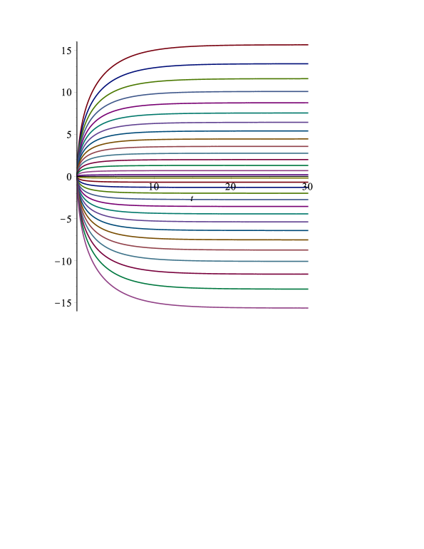
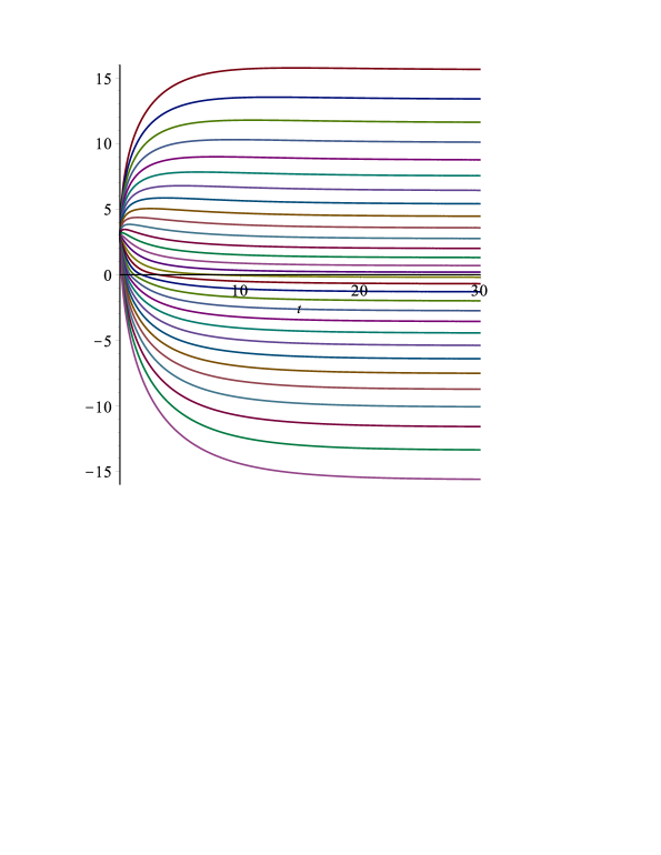
For $n=30$ with $a=10$ and $b=\frac{3}{10}$, the continuous Hahn roots become with a precision of 4 decimals:

$$\begin{matrix}x_{1}^{(30)}=-15.6230,&&x_{6}^{(30)}=-7.5285,&&x_{11}^{(30)}=-2.7503,\\ x_{2}^{(30)}=-13.3738,&&x_{7}^{(30)}=-6.4188,&&x_{12}^{(30)}=-1.9957,\\ x_{3}^{(30)}=-11.6001,&&x_{8}^{(30)}=-5.3956,&&x_{13}^{(30)}=-1.3059,\\ x_{4}^{(30)}=-10.0841,&&x_{9}^{(30)}=-4.4474,&&x_{14}^{(30)}=-0.6907,\\ x_{5}^{(30)}=-8.7415,&&x_{10}^{(30)}=-3.5671,&&x_{15}^{(30)}=-0.1919\end{matrix}$$

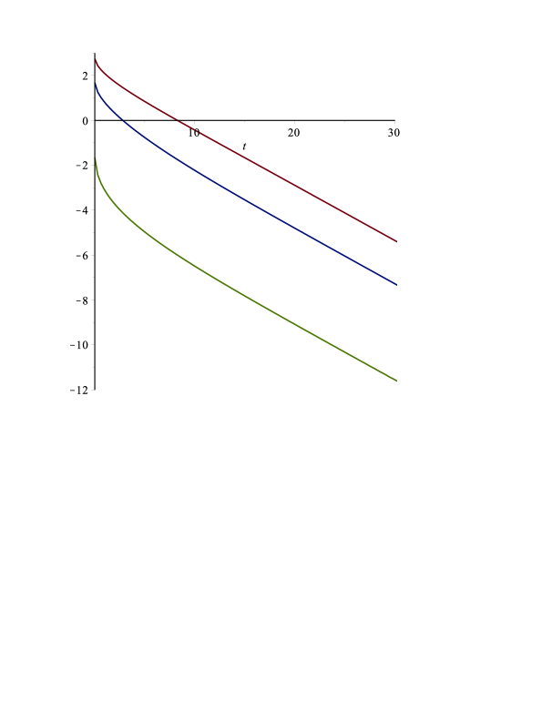
(and $x^{(30)}_{j}=-x^{(30)}_{31-j}$ for $j=16,\ldots,30$). The corresponding trajectories of $x_{j}^{(n)}(t)$ for $0\leq t\leq 30$ starting from the origin, i.e. with $x_{j}^{(n)}(0)=0$ ($j=1,\ldots,n$), are exhibited in Figure 1. The slope of the evolution of the logarithmic error $\log\bigl{|}x_{j}(t)-x_{j}^{(n)}\bigr{|}$ in Figure 2 confirms that the convergence is exponential with a decay rate that exceeds the not very sharp estimate of $\frac{a}{a^{2}+R_{n}^{2}}+\frac{b}{b^{2}+R_{n}^{2}}\approx 0.030$ guaranteed by Theorem 1.

Figure 1. Continuous Hahn trajectories $x^{(30)}_{1}(t),\ldots,x_{30}^{(30)}(t)$ corresponding to the initial condition $x_{j}^{(30)}(0)=0$ ($j=1,\ldots,30$) and the parameter values $a=10$ and $b=\frac{3}{10}$.

Figure 2. Evolution of the continuous Hahn logarithmic error $\log\bigl{|}x_{j}(t)-x_{j}^{(30)}\bigr{|}$ for $j=1$ (top), $j=8$ (middle) and $j=15$ (bottom), corresponding to the initial condition $x_{j}^{(30)}(0)=0$ ($j=1,\ldots,30$) and the parameter values $a=10$ and $b=\frac{3}{10}$.

3. Wilson Polynomials

3.1. Preliminaries

The monic Wilson polynomial $\text{p}_{n}(x^{2};a,b,c,d)$ [38] is an orthogonal polynomial of degree $n$ in $x^{2}$ that sits at the top of Askey’s hypergeometric scheme [25]. For generic parameter values it is given by the terminating hypergeometric series [25, Chapter 9.1]

$$\text{p}_{n}(x^{2};a,b,c,d)= \frac{(-1)^{n}(a+b,a+c,a+d)_{n}}{(n+a+b+c+d-1)_{n}}$$ (3.1)

$$\times{}_{4}F_{3}\left[\begin{array}[]{c}-n,n+a+b+c+d-1,a+ix,a-ix\\ a+b,a+c,a+d\end{array};1\right],$$ (3.4)

When $\text{Re}(a),\text{Re}(b),\text{Re}(c),\text{Re}(d)>0$ with possible non-real parameters arising in complex conjugate pairs, the polynomials in question satisfy the following orthogonality relations [25, Chapter 9.1]

$$\frac{1}{2\pi}\int_{0}^{\infty}\Delta(x;a,b,c,d)\text{p}_{n}(x^{2};a,b,c,d)\text{p}_{m}(x^{2};a,b,c,d)\text{d}x=$$ (3.5a)

$$\begin{cases}\frac{n!\Gamma(a+b+c+d+n-1)\Gamma(a+b+n)\Gamma(a+c+n)\Gamma(a+d+n)\Gamma(b+c+n)\Gamma(b+d+n)\Gamma(c+d+n)}{\Gamma(a+b+c+d+2n-1)\Gamma(a+b+c+d+2n)}&\ \text{if}\ m=n,\\ 0&\ \text{if}\ m\neq n,\end{cases}$$

where

$$\Delta(x;a,b,c,d)=\left|\frac{\Gamma(a+ix)\Gamma(b+ix)\Gamma(c+ix)\Gamma(d+ix)}{\Gamma(2ix)}\right|^{2}.$$ (3.5b)

3.2. Morse Function

For parameters values within the above orthogonality regime, the roots

$$0<x_{1}^{(n)}<x_{2}^{(n)}<\cdots<x_{n}^{(n)}$$

of the Wilson polynomial $\text{p}_{n}(x^{2};a,b,c,d)$ minimize the Morse function [12, Remarks 5.4, 5.5]

$$V(x_{1},\ldots,x_{n};a,b,c,d)=\sum_{1\leq j<k\leq n} \left(\int_{0}^{x_{j}+x_{k}}\arctan(\theta)\text{d}\theta+\int_{0}^{x_{j}-x_{k}}\arctan(\theta)\text{d}\theta\right)$$

$$+\sum_{1\leq j\leq n} \left(\int_{0}^{x_{j}}\arctan\left(\frac{\theta}{a}\right)+\arctan\left(\frac{\theta}{b}\right)\right.$$ (3.6)

$$\qquad\left.+\arctan\left(\frac{\theta}{c}\right)+\arctan\left(\frac{\theta}{d}\right)\text{d}\theta-\pi jx_{j}\right).$$

Indeed, we now have that at the critical points of the Morse function

$$\arctan\left(\frac{x_{j}}{a}\right) +\arctan\left(\frac{x_{j}}{b}\right)+\arctan\left(\frac{x_{j}}{c}\right)+\arctan\left(\frac{x_{j}}{d}\right)$$

$$+\sum_{\begin{subarray}{c}1\leq k\leq n\\ k\neq j\end{subarray}}\bigl{(}\arctan(x_{j}+x_{k})+\arctan(x_{j}-x_{k})\bigr{)}=\pi j$$

($j=1,\ldots,n$), so $0<x_{1}<x_{2}<\cdots<x_{n}$ and (after exponentiation)

$$\frac{\bigl{(}ia+x_{j}\bigr{)}\bigl{(}ib+x_{j}\bigr{)}\bigl{(}ic+x_{j}\bigr{)}\bigl{(}id+x_{j}\bigr{)}}{\bigl{(}ia-x_{j}\bigr{)}\bigl{(}ib-x_{k}\bigr{)}\bigl{(}ic-x_{j}\bigr{)}\bigl{(}id-x_{j}\bigr{)}}\prod_{\begin{subarray}{c}1\leq k\leq n\\ k\neq j\end{subarray}}\frac{(i+x_{j}+x_{k})(i+x_{j}-x_{k})}{(i-x_{j}-x_{k})(i-x_{j}+x_{k})}=1$$

for $j=1,\ldots,n$. Upon rewriting the latter identities in the form

$$A(x_{j};a,b,c,d)\text{p}_{n}(x_{j}+i)+A(-x_{j};a,b,c,d)\text{p}_{n}(x_{j}-i)=0\quad(j=1,\ldots,n),$$

with $A(x;a,b,c,d)=\frac{(x+ia)(x+ib)(x+ic)(x+id)}{2x(2x+i)}$ and

$$\text{p}_{n}(x)=(x^{2}-x^{2}_{1})(x^{2}-x^{2}_{2})\cdots(x^{2}-x^{2}_{n}),$$

it is deduced in the same way as before that the factorized polynomial in question satisfies the second-order difference equation for the Wilson polynomials [25, Chapter 9.1]:

$$A(x;a,b,c,d)\Bigl{(}\text{p}_{n}(x+i)-\text{p}_{n}(x)\Bigr{)}+$$

$$A(-x;a,b,c,d)\Bigl{(}\text{p}_{n}(x-i)-\text{p}_{n}(x)\Bigr{)}=\lambda_{n}\text{p}_{n}(x)$$

with $\lambda_{n}=-n(n+a+b+c+d-1)$. The upshot is that $\text{p}_{n}(x)=\text{p}_{n}(x^{2};a,b,c,d)$ (using again the nondegeneracy of the eigenvalues $\lambda_{n}$ at the RHS) and thus $x_{j}=x_{j}^{(n)}$ ($j=1,\ldots,n$).

Let us stress in this connection that the observation that the roots of Wilson polynomial $p_{n}(x^{2};a,b,c,d)$ satisfy the algebraic identities in the second equation below the Morse function (3.6) goes again back to [28] (cf. also [10] and [3]).

3.3. Gradient Flow

The corresponding gradient flow now becomes:

$${\frac{\text{d}x_{j}}{\text{d}t}-\pi j} +{\arctan\left(\frac{x_{j}}{a}\right)+\arctan\left(\frac{x_{j}}{b}\right)+\arctan\left(\frac{x_{j}}{c}\right)+\arctan\left(\frac{x_{j}}{d}\right)}$$ (3.7)

$$+\sum_{\begin{subarray}{c}1\leq k\leq n\\ k\neq j\end{subarray}}\bigl{(}\arctan(x_{j}+x_{k})+\arctan(x_{j}-x_{k})\bigr{)}=0,$$

$j=1,\ldots,n$. The following theorem affirms that the solutions of the gradient system (3.7) converge exponentially to the equilibrium $\bigl{(}x_{1}^{(n)},\ldots,x_{n}^{(n)}\bigr{)}$ given by the Wilson roots.

Theorem 2.

Let $$\text{Re}(a),\text{Re}(b),\text{Re}(c),\text{Re}(d)>0$$ with possible non-real parameters arising in complex conjugate pairs.

• The unique global minimum of the strictly convex, radially unbounded, Morse function $V(x_{1},\ldots,x_{n};a,b,c,d)$ (3.6) is attained at the Wilson roots $x_{j}=x_{j}^{(n)}$ ($j=1,\ldots,n$).

• Let $\bigl{(}x_{1}(t),\ldots,x_{n}(t)\bigr{)}$, $t\geq 0$ denote the unique solution of the gradient system (3.7) determined by a choice for the initial condition

  $$(x_{1}(0),\ldots,x_{n}(0))\in\mathbb{R}^{n},$$

  and let us fix any $\kappa$ in the interval

  $${\textstyle 0<\kappa<\frac{2(n-1)}{1+4R_{n}^{2}}+\frac{\text{Re}(a)}{\text{Re}^{2}(a)+(R_{n}+|\text{Im}(a)|)^{2}}+\frac{\text{Re}(b)}{\text{Re}^{2}(b)+(R_{n}+|\text{Im}(b)|)^{2}}}$$ (3.8a)

  $${\textstyle+\frac{\text{Re}(c)}{\text{Re}^{2}(c)+(R_{n}+|\text{Im}(c)|)^{2}}+\frac{\text{Re}(d)}{\text{Re}^{2}(d)+(R_{n}+|\text{Im}(d)|)^{2}}}$$

  where $R_{n}:=x_{n}^{(n)}$. Then there exists a constant $K>0$ (depending on the parameter values, on the initial condition, and on $\kappa$) such that

  $$|x_{j}(t)-x_{j}^{(n)}|\leq Ke^{-\kappa t}\qquad(j=1,\ldots,n)$$ (3.8b)

  whenever $t\geq 0$.

3.4. Proof of Theorem 2

The proof runs along the same lines as that of Theorem 1, so we only highlight some of the principal modifications in the corresponding computations.

As before, the first part of the theorem hinges on the considerations in [12, Remarks 5.4, 5.5] with the main points summarized above in Subsection 3.2 (cf. also the proof of [12, Proposition 4.1] for a detailed check that the present Morse function is indeed radially unbounded).

To infer the asserted estimate for the convergence rate, we must again provide the lower bound for the eigenvalues of the pertinent Jacobian evaluated at the equilibrium point. This Jacobian is given by the Hessian

$$H_{j,k}(x_{1},\ldots,x_{n};a,b,c,d)=\partial_{x_{j}}\partial_{x_{k}}V(x_{1},\ldots,x_{n};a,b,c,d)$$ (3.9)

$$=\begin{cases}\frac{a}{a^{2}+x_{j}^{2}}+\frac{b}{b^{2}+x_{j}^{2}}+\frac{c}{c^{2}+x_{j}^{2}}+\frac{d}{d^{2}+x_{j}^{2}}+\sum_{l\neq j}\bigl{(}\frac{1}{1+(x_{j}+x_{l})^{2}}+\frac{1}{1+(x_{j}-x_{l})^{2}}\bigr{)}&\text{if $j=k$,}\\ \frac{1}{1+(x_{j}+x_{l})^{2}}-\frac{1}{1+(x_{j}-x_{l})^{2}}&\text{if $j\neq k$,}\\ \end{cases}$$

which confirms the convexity:

$$\sum_{1\leq j,k\leq n}y_{j}y_{k}H_{j,k}(x_{1},\ldots,x_{n};a,b,c,d)=\sum_{1\leq j\leq n}\Bigl{(}\sum_{\epsilon\in\{a,b,c,d\}}\frac{\epsilon}{\epsilon^{2}+x_{j}^{2}}\Bigr{)}y_{j}^{2}$$

$$+\sum_{1\leq j<k\leq n}\Bigl{(}\frac{(y_{j}+y_{k})^{2}}{1+(x_{j}+x_{k})^{2}}+\frac{(y_{j}-y_{k})^{2}}{1+(x_{j}-x_{k})^{2}}\Bigr{)}.$$

Since $0<x_{j}\leq R_{n}$ ($j=1,\ldots,n$) at the equilibrium, we now see that

$$\sum_{1\leq j,k\leq n}y_{j}y_{k}H_{j,k}(x_{1}^{(n)},\ldots,x_{n}^{(n)};a,b,c,d)$$

$$\geq{\textstyle\left(\sum_{\epsilon\in\{a,b,c,d\}}\frac{\text{Re}(\epsilon)}{\text{Re}^{2}(\epsilon)+(R_{n}+|\text{Im}(\epsilon)|)^{2}}\right)(y_{1}^{2}+\cdots+y_{n}^{2})}$$

$$+\sum_{1\leq j<k\leq n}\frac{(y_{j}+y_{k})^{2}+(y_{j}-y_{k})^{2}}{1+4R_{n}^{2}}$$

$$={\textstyle\left(\sum_{\epsilon\in\{a,b,c,d\}}\frac{\text{Re}(\epsilon)}{\text{Re}^{2}(\epsilon)+(R_{n}+|\text{Im}(\epsilon)|)^{2}}+\frac{2(n-1)}{1+4R_{n}^{2}}\right)(y_{1}^{2}+\cdots+y_{n}^{2})}.$$

This entails the desired lower bound for the smallest eigenvalue:

$$\lambda =\min_{\begin{subarray}{c}(y_{1},\ldots,y_{n})\in\mathbb{R}^{n}\\ y_{1}^{2}+\cdots+y_{n}^{2}\neq 0\end{subarray}}\frac{\sum_{1\leq j,k\leq n}y_{j}y_{k}H_{j,k}(x_{1}^{(n)},\ldots,x_{n}^{(n)};a,b,c,d)}{y_{1}^{2}+\cdots+y_{n}^{2}}$$

$$\geq\sum_{\epsilon\in\{a,b,c,d\}}\frac{\text{Re}(\epsilon)}{\text{Re}^{2}(\epsilon)+(R_{n}+|\text{Im}(\epsilon)|)^{2}}+\frac{2(n-1)}{1+4R_{n}^{2}}>\kappa.$$

3.5. Numerical Samples

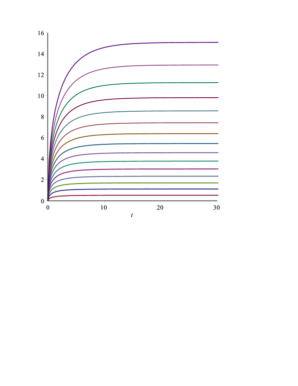
For $n=15$ with $a=\frac{17}{3}$, $b=\frac{1}{5}$, $c=1+i$, and $d=1-i$, the Wilson roots become with a precision of 4 decimals:

$$\begin{matrix}x_{1}^{(15)}=0.5274,&&x_{6}^{(15)}=3.7728,&&x_{11}^{(15)}=8.5546,\\ x_{2}^{(15)}=1.1194,&&x_{7}^{(15)}=4.5787,&&x_{12}^{(15)}=9.8143,\\ x_{3}^{(15)}=1.7050,&&x_{8}^{(15)}=5.4496,&&x_{13}^{(15)}=11.2449,\\ x_{4}^{(15)}=2.3375,&&x_{9}^{(15)}=6.3938,&&x_{14}^{(15)}=12.9284,\\ x_{5}^{(15)}=3.0266,&&x_{10}^{(15)}=7.4231,&&x_{15}^{(15)}=15.0759.\end{matrix}$$

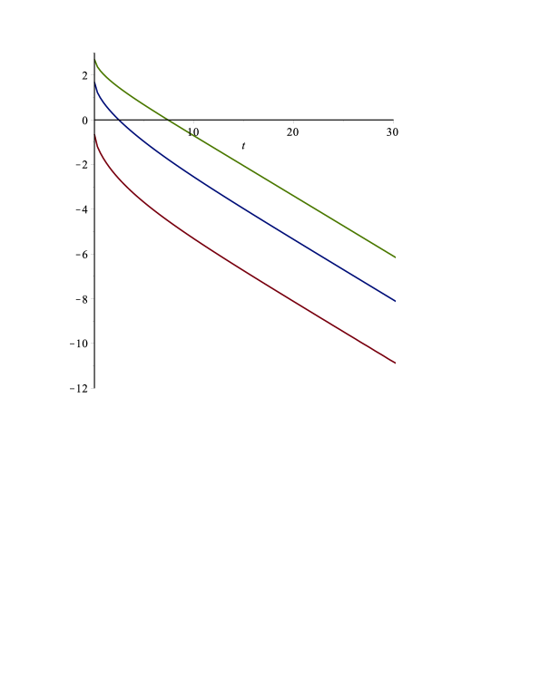
The corresponding trajectories of $x_{j}^{(n)}(t)$ for $0\leq t\leq 30$, with an initial condition of the form $x_{j}^{(n)}(0)=0$ ($j=1,\ldots,n$), are exhibited in Figure 3. The slope of the evolution of the logarithmic error $\log\bigl{|}x_{j}(t)-x_{j}^{(n)}\bigr{|}$ in Figure 4 confirms that the convergence is exponential with a decay rate that exceeds the not very sharp estimate of

$$\sum_{\epsilon\in\{a,b,c,d\}}\frac{\text{Re}(\epsilon)}{\text{Re}^{2}(\epsilon)+(R_{n}+|\text{Im}(\epsilon)|)^{2}}+\frac{2(n-1)}{1+4R_{n}^{2}}\approx 0.061$$

guaranteed by Theorem 2.

Figure 3. Wilson trajectories $x^{(15)}_{1}(t),\ldots,x_{15}^{(15)}(t)$ corresponding to the initial condition $x_{j}^{(15)}(0)=0$ ($j=1,\ldots,15$) and the parameter values $a=\frac{17}{3}$, $b=\frac{1}{5}$, $c=1+i$, and $d=1-i$.

Figure 4. Evolution of the Wilson logarithmic error $\log\bigl{|}x_{j}(t)-x_{j}^{(15)}\bigr{|}$ for $j=1$ (bottom), $j=8$ (middle) and $j=15$ (top), corresponding to the initial condition $x_{j}^{(15)}(0)=0$ ($j=1,\ldots,15$) and the parameter values $a=\frac{17}{3}$, $b=\frac{1}{5}$, $c=1+i$, and $d=1-i$.

4. Symmetry Reduction

As noticed above, the weight function $\Delta(x;a,b)$ (2.5b) is even in $x$ for our parameter regime, so the roots of the corresponding symmetric continuous Hahn polynomial $\text{p}_{n}(x;a,b)$ are symmetrically distributed around the origin:

$$x_{j}^{(n)}+x_{n+1-j}^{(n)}=0\quad\text{for}\ j=1,\ldots,n.$$ (4.1)

It is manifest from the explicit differential equations that the gradient system in Eqs. (2.9a), (2.9b) preserves this parity symmetry. More specifically, if the initial condition satisfies

$$x_{j}(0)+x_{n+1-j}(0)=0\quad\text{for}\ j=1,\ldots,n,$$ (4.2a)

then so does the corresponding gradient flow $$\bigl{(}x_{1}(t),\ldots,x_{n}(t)\bigr{)} t\geq 0$$, :

$$x_{j}(t)+x_{n+1-j}(t)=0\quad\text{for}\ j=1,\ldots,n.$$ (4.2b)

If we now perform the reduction of our gradient system to the pertinent $m:=\lfloor\frac{n}{2}\rfloor$-dimensional invariant manifold through the substitution

$$(x_{1},\ldots,x_{n})=\begin{cases}(-y_{m},\ldots,-y_{1},y_{1},\ldots,y_{m})&\text{if}\ n=2m,\\ (-y_{m},\ldots,-y_{1},0,y_{1},\ldots,y_{m})&\text{if}\ n=2m+1,\end{cases}$$ (4.3)

then we arrive at the differential equations

$${\frac{\text{d}y_{j}}{\text{d}t}-\pi(j-{\textstyle\frac{1}{2}})} +{\arctan\left(\frac{y_{j}}{a}\right)+\arctan\left(\frac{y_{j}}{b}\right)+\arctan\left(2y_{j}\right)}$$ (4.4a)

$$+\sum_{\begin{subarray}{c}1\leq k\leq m\\ k\neq j\end{subarray}}\bigl{(}\arctan(y_{j}+y_{k})+\arctan(y_{j}-y_{k})\bigr{)}=0$$

($$j=1,\ldots,m n=2m$$) when , and

$${\frac{\text{d}y_{j}}{\text{d}t}-\pi j} +{\arctan\left(\frac{y_{j}}{a}\right)+\arctan\left(\frac{y_{j}}{b}\right)+\arctan\left(2y_{j}\right)+\arctan\left(y_{j}\right)}$$ (4.4b)

$$+\sum_{\begin{subarray}{c}1\leq k\leq m\\ k\neq j\end{subarray}}\bigl{(}\arctan(y_{j}+y_{k})+\arctan(y_{j}-y_{k})\bigr{)}=0$$

($j=1,\ldots,m$) when $n=2m+1$, respectively. By comparing the latter differential equations with the gradient system for the Wilson polynomials in Eq. (3.7), it is seen that for $n=2m$ we recover the case $(a,b,c,d)\to(a,b,\frac{1}{2},0)$ and for $n=2m+1$ we recover the case $(a,b,c,d)\to(a,b,\frac{1}{2},1)$. Indeed, the symmetric continuous Hahn polynomials and the Wilson polynomials are known to be related by the following quadratic relations (cf. e.g. [26, Section 2.4]):

$$\text{p}_{n}(x;a,b)=\begin{cases}\text{p}_{m}(x^{2};a,b,\frac{1}{2},0)&\text{if}\ n=2m,\\ x\text{p}_{m}(x^{2};a,b,\frac{1}{2},1)&\text{if}\ n=2m+1.\end{cases}$$ (4.5)

The upshot is that for initial conditions respecting the parity invariance, the estimate for the rate of the exponential convergence in the second part of Theorem 1 can be improved as follows.

Theorem 3.

Let $$\text{Re}(a),\text{Re}(b)>0 a b \bigl{(}x_{1}(t),\ldots,x_{n}(t)\bigr{)} t\geq 0 (x_{1}(0),\ldots,x_{n}(0))\in\mathbb{R}^{n}$$ with possible non-real parameters and arising as a complex conjugate pair, and let , denote the unique solution of the gradient system (2.9a), (2.9b) determined by a choice for the initial condition such that

$$x_{j}(0)+x_{n+1-j}(0)=0\quad\text{for}\ j=1,\ldots,n.$$

Then for any $$\kappa$$ in the interval

$${\textstyle 0<\kappa<\frac{2\lfloor\frac{n}{2}\rfloor}{1+4R_{n}^{2}}+\frac{\text{Re}(a)}{\text{Re}^{2}(a)+(R_{n}+|\text{Im}(a)|)^{2}}+\frac{\text{Re}(b)}{\text{Re}^{2}(b)+(R_{n}+|\text{Im}(b)|)^{2}}}{\textstyle+\frac{1-(-1)^{n}}{2+2R_{n}^{2}}},$$ (4.6a)

where $$R_{n}:=x_{n}^{(n)} K>0 \kappa$$, there exists a constant (depending on the parameter values, on the initial condition, and on ) such that

$$|x_{j}(t)-x_{j}^{(n)}|\leq Ke^{-\kappa t}\qquad(j=1,\ldots,n)$$ (4.6b)

whenever $$t\geq 0$$.

For $n=2m+1$, Theorem 3 is immediate from the reduced differential equation (4.4b) and the second part of Theorem 2, upon performing the parameter specialization $(a,b,c,d)\to(a,b,\frac{1}{2},1)$. The case $n=2m$ would follow similarly via the reduced differential equation (4.4a) upon performing the parameter specialization $(a,b,c,d)\to(a,b,\frac{1}{2},0)$ in Theorem 2. However, since the parameter specialization $d\to 0$ takes us outside the Wilson parameter domain considered here, for the argument to stick rigorously one formally has to repeat the proof of Theorem 2 for the case of the gradient flow in Eq. (4.4a).

Since our numerical example in Section 2.5 corresponded to an initial condition of the form $x_{j}(0)=0$ ($j=1,\ldots,n$), the improved exponential convergence of Theorem 3 actually applies in this situation. However, if we break the parity symmetry by moving the initial condition up to $x_{j}(0)=3$ ($j=1,\ldots,n$)—while maintaining the parameter values $a=10$ and $b=\frac{3}{10}$ (cf. Figure 5)—then we see from the slopes of the logarithmic error (cf. Figure 6) that the rate of the exponential convergence indeed slows down considerably. Notice at this point that the downward peaks in the evolution of the logarithmic error reveal that the corresponding limiting values are no longer approached monotonously: the peak detects when the trajectory of $x_{j}(t)$ overshoots its limiting value $x_{j}^{(n)}$.

Figure 5. Continuous Hahn trajectories $x^{(30)}_{1}(t),\ldots,x_{30}^{(30)}(t)$ corresponding to the initial condition $x_{j}^{(30)}(0)=3$ ($j=1,\ldots,30$) and the parameter values $a=10$ and $b=\frac{3}{10}$.

Figure 6. Evolution of the continuous Hahn logarithmic error $\log\bigl{|}x_{j}(t)-x_{j}^{(30)}\bigr{|}$ for $j=1$ (top), $j=8$ (second from below), $j=23$ (bottom), and $j=30$ (second from above), where the ordering refers to that of the asymptotic tails, with the initial condition $x_{j}^{(30)}(0)=3$ ($j=1,\ldots,30$) and the parameter values $a=10$ and $b=\frac{3}{10}$.

References

- [1] Askey, R., Wilson, J.: A set of hypergeometric orthogonal polynomials. SIAM J. Math. Anal. 13, 651–655 (1982)
- [2] Beltrán, C., Marcellán, F., Martínez-Finkelshtein, A.: Some extremal properties of the roots of orthogonal polynomials. Gac. R. Soc. Mat. Esp. 21, 345–366 (2018)
- [3] Bihun, O., Calogero, F.: Properties of the zeros of the polynomials belonging to the Askey scheme. Lett. Math. Phys. 104, 1571–1588 (2014)
- [4] Bihun, O., Calogero, F.: Properties of the zeros of the polynomials belonging to the -Askey scheme. J. Math. Anal. Appl. 433, 525–542 (2016)
- [5] Calogero, F.: Equilibrium configuration of the one-dimensional -body problem with quadratic and inversely quadratic pair potentials. Lett. Nuovo Cimento (2) 20, 251–253 (1977).
- [6] Chicone, C.: Ordinary Differential Equations with Applications. Second Edition, Springer, New York (2006)
- [7] van Diejen, J.F.: Deformations of Calogero-Moser systems and finite Toda chains. Theoret. and Math. Phys. 99, 549–554 (1994)
- [8] van Diejen, J.F.: Difference Calogero-Moser systems and finite Toda chains. J. Math. Phys. 36, 1299–1323 (1995)
- [9] van Diejen, J.F.: Multivariable continuous Hahn and Wilson polynomials related to integrable difference systems. J. Phys. A 28, L369–L374 (1995)
- [10] van Diejen, J.F.: On the equilibrium configuration of the -type Ruijsenaars-Schneider system. J. Nonlinear Math. Phys. 12, suppl. 1, 689–696 (2005)
- [11] van Diejen, J.F.: Gradient system for the roots of the Askey-Wilson polynomial. Proc. Amer. Math. Soc. 147, 5239–5249 (2019)
- [12] van Diejen, J.F., Emsiz, E.: Solutions of convex Bethe Ansatz equations and the zeros of (basic) hypergeometric orthogonal polynomials. Lett. Math. Phys. 109, 89–112 (2019)
- [13] Dimitrov, D.K., Van Assche, W.: Lamé differential equations and electrostatics. Proc. Amer. Math. Soc. 128, 3621–3628 (2000)
- [14] Fehér, L., Görbe, T.F.: Duality between the trigonometric Sutherland system and a completed rational Ruijsenaars-Schneider-van Diejen system. J. Math. Phys. 55, no. 10, 102704 (2014)
- [15] Forrester, P.J., Rogers, J.B.: Electrostatics and the zeros of the classical polynomials. SIAM J. Math. Anal. 17, 461–468 (1986)
- [16] Grünbaum, F.A.: Variations on a theme of Heine and Stieltjes: an electrostatic interpretation of the zeros of certain polynomials. J. Comput. Appl. Math. 99, 189–194 (1998)
- [17] Grünbaum, F.A.: Electrostatic interpretation for the zeros of certain polynomials and the Darboux process. J. Comput. Appl. Math. 133, 397–412 (2001)
- [18] Hendriksen, E., van Rossum, H., Electrostatic interpretation of zeros. In: Orthogonal Polynomials and their Applications, pp. 241–250, Lecture Notes in Math. 1329, Springer, Berlin (1988)
- [19] Horváth, Á.P.: The electrostatic properties of zeros of exceptional Laguerre and Jacobi polynomials and stable interpolation. J. Approx. Theory 194, 87–107 (2015)
- [20] Ismail, M.E.H.: An electrostatics model for zeros of general orthogonal polynomials. Pacific J. Math. 193, 355–369 (2000)
- [21] Ismail, M.E.H.: More on electrostatic models for zeros of orthogonal polynomials. Numer. Funct. Anal. Optim. 21, 191–204 (2000)
- [22] Ismail, M.E.H.: Classical and Quantum Orthogonal Polynomials in One Variable. Cambridge University Press, Cambridge (2005)
- [23] Jooste, A., Njionou Sadjang, P., Koepf, W.: Inner bounds for the extreme zeros of hypergeometric polynomials. Integral Transforms Spec. Funct. 28, 361–373 (2017)
- [24] Khalil, H.K.: Nonlinear Systems. Third Edition, Prentice Hall, Upper Saddle River, N.J. (2002)
- [25] Koekoek, R., Lesky, P.A., Swarttouw, R.: Hypergeometric Orthogonal Polynomials and their q-Analogues. Springer, Berlin (2010)
- [26] Koornwinder, T.H.: Quadratic transformations for orthogonal polynomials in one and two variables. In: Representation Theory, Special Functions and Painlevé Equations–RIMS 2015, pp. 419–447, Adv. Stud. Pure Math. 76, Math. Soc. Japan, Tokyo (2018)
- [27] Marcellán, F., Martínez-Finkelshtein, A., Martínez-González, P.: Electrostatic models for zeros of polynomials: old, new, and some open problems. J. Comput. Appl. Math. 207, 258–272 (2007)
- [28] Odake, S., Sasaki, R.: Equilibria of ‘discrete’ integrable systems and deformation of classical orthogonal polynomials. J. Phys. A 37, 11841–11876 (2004)
- [29] Odake, S., Sasaki, R.: Equilibrium positions, shape invariance and Askey-Wilson polynomials. J. Math. Phys. 46, no. 6, 063513 (2005)
- [30] Odake, S., Sasaki, R.: Calogero-Sutherland-Moser systems, Ruijsenaars-Schneider-van Diejen systems and orthogonal polynomials. Prog. Theor. Phys. 114, 1245–1260 (2005)
- [31] Perelomov, A.M.: Equilibrium configurations and small oscillations of some dynamical systems. Ann. Inst. H. Poincaré Sect. A (N.S.) 28, 407–415 (1978)
- [32] Pusztai, B.G.: The hyperbolic Sutherland and the rational Ruijsenaars-Schneider-van Diejen models: Lax matrices and duality. Nuclear Phys. B 856, 528–551 (2012)
- [33] Pusztai, B.G.: Scattering theory of the hyperbolic Sutherland and the rational Ruijsenaars-Schneider-van Diejen models. Nuclear Phys. B 874, 647–662 (2013)
- [34] Simanek, B.: An electrostatic interpretation of the zeros of paraorthogonal polynomials on the unit circle. SIAM J. Math. Anal. 48, 2250–2268 (2016)
- [35] Steinerberger, S.: Electrostatic interpretation of zeros of orthogonal polynomials. Proc. Amer. Math. Soc. 146, 5323–5331 (2018)
- [36] Stieltjes, T.J.: Sur certains polynômes qui vérifient une équation différentielle linéaire du second ordre et sur la theorie des fonctions de Lamé. Acta Math. 6, 321–326 (1885)
- [37] Szegö, G.: Orthogonal Polynomials. Fourth Edition, American Mathematical Society, Providence, R.I. (1975)
- [38] Wilson, J.A.: Some hypergeometric orthogonal polynomials. SIAM J. Math. Anal. 11, 690–701 (1980)