Ultrafast Wave-Particle Energy Transfer in the Collapse of Standing Whistler Waves

Abstract

Efficient energy transfer from electromagnetic waves to ions has been demanded to control laboratory plasmas for various applications and could be useful to understand the nature of space and astrophysical plasmas. However, there exists a severe unsolved problem that most of the wave energy is converted quickly to electrons, but not to ions. Here, an energy conversion process to ions in overdense plasmas associated with whistler waves is investigated by numerical simulations and theoretical model. Whistler waves propagating along a magnetic field in space and laboratories often form the standing waves by the collision of counter-propagating waves or through the reflection. We find that ions in the standing whistler waves acquire a large amount of energy directly from the waves in a short timescale comparable to the wave oscillation period. Thermalized ion temperature increases in proportion to the square of the wave amplitude and becomes much higher than the electron temperature in a wide range of wave-plasma conditions. This efficient ion-heating mechanism applies to various plasma phenomena in space physics and fusion energy sciences.

I Introduction

Plasma acceleration and heating by electromagnetic waves is of great importance in many research topics such as parametric instabilities Kruer (2003), collisionless shocks and turbulence Lembege et al. (2004), planetary magnetospheres Stenzel (1999, 2016), and inertial and magnetic confinement fusion (ICF and MCF) Lindl (1995); Betti and Hurricane (2016); Stacey (2005). Among different types of waves, the whistler wave, which is a low-frequency electromagnetic wave traveling along an external magnetic field $B_{\rm ext}$, often plays a major role in the generation of energetic particles Stenzel (1999, 2016). Whistler-mode chorus waves are one of the most intense plasma waves observed in planetary magnetospheres Helliwell (1965); Tsurutani and Smith (1974); Coroniti et al. (1980); Hospodarsky et al. (2008); Artemyev et al. (2016) and expected as a promising mechanism to produce relativistic electrons Horne et al. (2005); Omura et al. (2007); Summers and Omura (2007); Thorne et al. (2013). Whistler waves are considered useful for inducing plasma currents and heating electrons in tokamak devices for MCF Stacey (2005); Prater et al. (2014) and also generated in laser plasmas of ICF experiments Mourenas (1998); Taguchi et al. (2017).

The whistler wave is a right-hand circularly polarized (CP) light permitted to exist when the electron cyclotron frequency $\omega_{ce}=eB_{\rm ext}/m_{e}$ exceeds that of the electromagnetic wave $\omega_{0}$, where $e$ is the elementary charge and $m_{e}$ is the electron mass. The critical field strength $B_{c}$ is defined by $B_{c}\equiv m_{e}\omega_{0}/e$ assuming $\omega_{0}=\omega_{ce}$. Note that the required magnetic field becomes weaker if the whistler frequency is lower or the wavelength is longer.

The whistler wave has interesting characteristics that give an advantage to plasma heating processes. The most important feature is no cutoff density for the whistler waves. Whistler waves can propagate inside of any density plasmas unless they encounter a strong density gradient so that they interact directly even with overdense plasmas Yang et al. (2015); Ma et al. (2016); Weng et al. (2017). Another critical fact is that a large electromotive potential, or an electrostatic potential, in the longitudinal direction appears in the standing wave of whistler-mode. The standing waves are naturally excited by overlapping two counter-propagating waves or by the reflection at the discontinuity of plasma density. The rapid build-up of the electrostatic potential accelerates ions. The amplitude of the potential energy is roughly given by $\psi\sim ev_{w}B_{w}\lambda_{w}/(2\pi)$, where $v_{w}$, $B_{w}$, and $\lambda_{w}$ are the amplitude of velocity, magnetic field, and wavelength of a whistler wave. The potential energy could be of the order of MeV for the relativistic whistler cases, and thus it is an attractive source for the energy transfer from the waves to plasmas. Nevertheless, the details of plasma acceleration and heating during the interaction between the standing whistler waves and overdense plasmas have not been examined yet.

In this paper, we focus on the ion-heating mechanism by standing whistler waves. The polarization direction of the electric field in whistler waves is the same as the cyclotron motion of electrons. When the wave frequency is close to the cyclotron frequency, $B_{\rm ext}\sim B_{c}$, electrons get the kinetic energy dramatically through the resonance Sano et al. (2017), and almost all the wave energy is converted to the electrons. The external magnetic field considered here is larger than the critical value, $B_{\rm ext}>B_{c}$, to avoid the electron cyclotron resonance Sano et al. (2017). In the propagation of whistler waves, the stimulated Brillouin scattering takes place, and which reduces the wave energy and drives ion-acoustic waves Nishikawa (1968); Forslund et al. (1972); Lee (1974). However, the growth rate of the parametric decay instability is usually much lower than the wave frequency. In order to concentrate only on faster processes of energy conversion, the duration of whistler waves in this analysis is limited to a few tens of the wave periods.

We find that a substantial fraction of the wave energy is transferred to ions as a result of the formation and immediate collapse of standing whistler waves. This mechanism is different from stochastic heating of underdense plasmas by a large-amplitude standing wave Hsu et al. (1979); Doveil (1981); Tran (1982). Our mechanism works only in overdense plasmas, and catalytic behavior of electron fluid is essential for the ion heating. Hereafter, we demonstrate the ultrafast ion-heating process by one-dimensional (1D) Particle-in-Cell (PIC) simulations. We also construct a theoretical model of the heating mechanism and then derive an analytical prescription of the ion temperature achieved by the standing whistler wave heating. Finally, prospective applications of our heating mechanism are discussed.

II Numerical demonstration of standing whistler wave heating

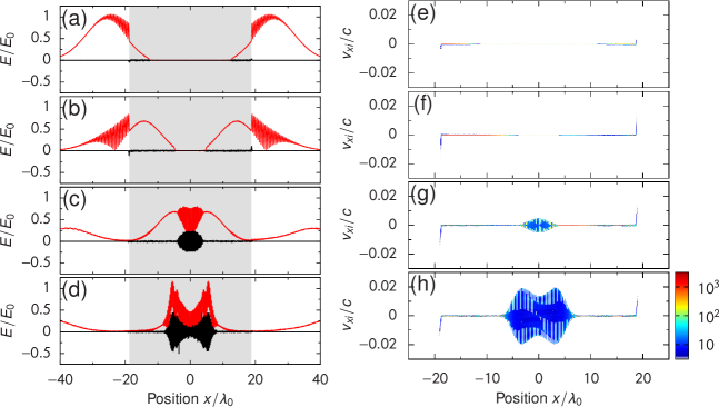
Figure 1: Snapshots of the electric fields and ion phase diagram in the 1D PIC simulation of the interaction between counter whistler waves and plasmas. (a–d) Time evolution of the electric fields during counter irradiation of circularly polarized lights. The longitudinal and tangential fields ($E_{x}$ and $|\bm{E}_{\perp}|$) are depicted by the black and red curves, respectively. Snapshot data are taken at (a) $\omega_{0}t=-4.71$, (b) 73.8, (c) 152, and (d) 192, where the origin of time $t=0$ is defined by the timing when the injected lights arrive at the target surface. The gray area stands for the inside of the target layer. (e–h) Snapshots of the position-velocity ($x$-$v_{xi}$) phase diagram for ions taken at the same timing as in (a)-(d). The color denotes the particle numbers.

A simple way to form a standing electromagnetic wave is by the use of two counter beams. Consider a thin layer of cold hydrogen plasma in the vacuum irradiated by CP lights with the same frequency $\omega_{0}$ and wavelength $\lambda_{0}$ from both sides. In the fiducial run, the thickness of the target layer is $\widetilde{L}_{x}\equiv L_{x}/\lambda_{0}=37.5$. As for the initial setup, the hydrogen plasma target is located at $|x|\leq L_{x}/2$ and the outside of the target is the vacuum region. The electron density in the target is set to be overdense $\widetilde{n}_{e0}\equiv n_{e0}/n_{c}=19.3$, where $n_{c}=\epsilon_{0}m_{e}\omega_{0}^{2}/e^{2}$ is the critical density, $\epsilon_{0}$ is the vacuum permittivity. For simplicity, the target temperature is set to be zero initially, and we ignore the existence of the pre-plasma. A uniform external magnetic field is applied in the direction of the wave propagation axis $x$ and the strength is supercritical $\widetilde{B}_{\rm ext}\equiv B_{\rm ext}/B_{c}=7.47$, which is constant in time throughout the computation in 1D situations. The light traveling in the $x$ ($-x$) direction is right-hand (left-hand) CP to the propagation direction. In other words, both have right-hand polarization in terms of the magnetic field direction, and thus they enter the overdense target as the whistler waves Luan et al. (2016). The amplitude of the incident electromagnetic wave $E_{0}$ is characterized by the normalized vector potential $a_{0}=eE_{0}/(m_{e}c\omega_{0})$ where $c$ is the speed of light. The intensity of a CP light is expressed as $I_{0}=\epsilon_{0}cE_{0}^{2}$. A relativistic intensity with $a_{0}=2.65$ is considered and the wave envelope shape is Gaussian with the duration of $\omega_{0}\tau_{0}=70.6$.

The wave-plasma interaction is solved by a PIC scheme, PICLS Sentoku and Kemp (2008), including the Coulomb collisions. The escape boundary conditions for waves and particles are adopted for both sides of the boundaries. The CP waves are injected from both boundaries of the computational domain, which is sufficiently broader than the target thickness. Then the waves propagate in the vacuum for a while and then hit the target. The transmittance and reflectivity at the target surface depends on the refractive index of the whistler-mode $N=[1+\widetilde{n}_{e0}/(\widetilde{B}_{\rm ext}-1)]^{1/2}$, which is $N=2.00$ for the fiducial parameters. Because the collision term is scale dependent, the physical parameters of this run correspond to $L_{x}=30$ $\mu$m, $n_{e0}=3.37\times 10^{22}$ cm^-3, $B_{\rm ext}=100$ kT, $I_{0}=3\times 10^{19}$ W/cm², and $\tau_{0}=30$ fs by choosing the wavelength $\lambda_{0}=0.8$ $\mu$m. Here the electromagnetic wave conditions are determined based on the typical quantities for a TW-class femtosecond laser and the target density is equivalent to the solid hydrogen.

The spatial and temporal resolution is $\Delta x=c\Delta t=\lambda_{0}/10^{3}$ and the particle number is 200 per each grid cell at the beginning. In the strongly magnetized plasmas, the time resolution $\Delta t$ should be shorter than the electron gyration time as well as the plasma oscillation time. Otherwise, the unphysical numerical heating breaks the energy conservation. In order to capture the propagation of the whistler waves and the evolution of the standing waves correctly, it would be better for the whistler wavelength to be resolved by a few hundreds of grid cells. These conditions are satisfied in all simulations shown in this paper. We have confirmed by the convergence check that the conclusions discussed in our analysis are unaffected by the numerical resolution.

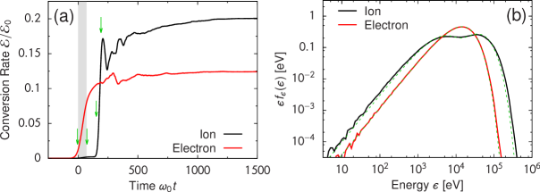
Figure 2: Energy conversion rate and energy spectra for ions and electrons in the fiducial run. (a) Time histories of the ion and electron energies normalized by the injected energy of the electromagnetic wave ${\cal{E}}_{0}$. The gray color in the figure stands for the pulse duration of the target irradiation, $0\leq\omega_{0}t\leq 70.6$. The arrows indicate the snapshot timing shown in Fig. 1. (b) Energy spectra for the ions and electrons at the end of the calculation. The vertical axis is $\epsilon f_{\epsilon}(\epsilon)$ where $f_{\epsilon}(\epsilon)$ is the probability density function for the energy $\epsilon$, so that the peak value is related to the temperature as $\epsilon_{\rm peak}=(3/2)k_{B}T$ in the Maxwell-Boltzmann distribution. The ion spectrum is fitted well by two temperature model with $T_{i}=24$ and $2.9$ keV, and the electron spectrum is almost identical to the thermal distribution of $T_{e}=9.6$ keV. The dotted curves show the fitted functions.

The PIC simulation clearly shows that ions in the overdense target are heated efficiently by the counter irradiation of CP lights. Because of the no-cutoff feature, both of the counter beams propagate inside of the target as whistler waves. When the two whistler waves pass each other, a standing whistler wave is formed in the middle of the target (Fig. 1). Right after the appearance of the standing wave, the longitudinal electric field $E_{x}$ is generated to the similar order of the transverse wave field $E_{0}$. At the same time, ions start to be accelerated by the electric field $E_{x}$. The ion velocity increases quickly up to 2% of the light speed within several wave periods. The rapid increase of ion energy can be seen in Fig. 2(a) where temporal histories of the total amount of energies for ions and electrons are depicted. When the injected wave fields step into the target layer, only electrons start to move due to the quiver motions of the whistler waves, whereas ion motion exhibits little change. However, the ion energy is jumped up at the timing when two whistler waves are overlapped at the center of the target, and ultimately the ion energy exceeds the electron energy. One-third of the wave energy is absorbed by plasmas through this interaction, where the ions gain more than 60% of the absorbed energy, i.e., the conversion efficiency from the waves to ions is $\sim$ 20%. The acquired ion energy is drastically enhanced by an order of magnitude compared with the case without the external magnetic field, or no whistler-mode case.

The energy spectrum of ions is nearly thermalized at the later stage far beyond the pulse duration, $\omega_{0}t_{\rm end}=2.78\times 10^{3}\gg\omega_{0}\tau_{0}$ [Fig. 2(b)]. The peak energy of the ion spectrum corresponds to about $T_{i}\sim 24$ keV, which is higher than the electron temperature of $T_{e}\sim 9.6$ keV. The energy density of the external magnetic field is still larger than that of the thermalized plasma. The plasma beta is about 0.02 at the end of calculation for this case.

This series of events is the ion-heating scenario by standing whistler waves in the numerical simulation. Surprisingly, thermal ion plasma over tens of keV in solid density is produced by Joule-class lasers in a rather simple geometry only if a sufficiently strong magnetic field is available.

III Theoretical modeling

Next, we will give a theoretical model of the ion-heating mechanism based on fundamental equations. The relativistic effects are neglected in the following analytical discussion. Eventually, it turns out that the ion temperature heated by counter whistler waves is described by a simple formula of the initial wave-plasma conditions.

The eigen functions of the tangential electric field $\bm{E}_{w}$, magnetic field $\bm{B}_{w}$ and electron velocity $\bm{v}_{w}$ for counter whistler waves traveling in the $\pm x$ direction with the wavenumber $k_{w}\equiv 2\pi/\lambda_{w}$ are given by

$$\bm{E}_{w}^{\pm} = E_{w}^{\pm}\exp\left[i\left(\pm k_{w}x-\omega_{0}t\right)\right](\widehat{y}+i\widehat{z})\;,$$ (1)

$$\bm{B}_{w}^{\pm} = \mp B_{w}^{\pm}\exp[i(\pm k_{w}x-\omega_{0}t)](i\widehat{y}-\widehat{z})\;,$$ (2)

$$\bm{v}_{w}^{\pm} = v_{w}^{\pm}\exp[i(\pm k_{w}x-\omega_{0}t)](i\widehat{y}-\widehat{z})\;,$$ (3)

where $B_{w}^{\pm}=({k_{w}}/{\omega_{0}})E_{w}^{\pm}$ and

$$v_{w}^{\pm}=\frac{1}{\widetilde{B}_{\rm ext}-1}\frac{e}{m_{e}\omega_{0}}E_{w}^{\pm}\;.$$ (4)

Suppose both of the injected CP lights have the same wavenumber $k_{0}$ and amplitude $a_{0}$ in the vacuum, the transmitted whistler waves will have $k_{w}=Nk_{0}$ and $a_{w}=2a_{0}/(N+1)$ Luan et al. (2016). Since $N$ is larger than unity when $B_{\rm ext}$ is supercritical, the wavelength and amplitude of the electromagnetic waves become shorter and smaller in the target. The nonrelativistic condition is then given by $a_{w}<\widetilde{B}_{\rm ext}-1$ from Eq. (4).

Let us consider the force balance for the electron fluid in the longitudinal direction. The electromotive force, $-e(\bm{v}_{e}\bm{\times}\bm{B})_{x}$, applied to the electrons is always zero, that is, $(\bm{v}_{w}^{\pm}\bm{\times}\bm{B}_{w}^{\pm})_{x}=0$ for the case of a single whistler wave. However, this term becomes finite in the standing whistler wave, $[(\bm{v}_{w}^{+}+\bm{v}_{w}^{-})\bm{\times}(\bm{B}_{w}^{+}+\bm{B}_{w}^{-})]_{x}\neq 0$, which brings curious consequence in the evolution of plasmas located at the standing wave.

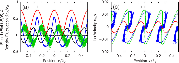
Figure 3: Detailed structures of a standing whistler wave and linearly growing velocity fluctuations of ions in the fiducial run. (a) Magnified view of the electric fields at the center of the target, $E_{x}$ (black) and $|\bm{E}_{\perp}|$ (red), taken at $\omega_{0}t=152$, which is right after the formation of the standing whistler wave. The electromotive field $(\bm{v}_{e}\bm{\times}\bm{B})_{x}$ worked on the electrons is also plotted by green dots. The blue curve denotes the electron density fluctuation $\delta n_{e}\equiv n_{e}-n_{e0}$. The length indicated in the figure corresponds to the wavelength of the whistler wave $\lambda_{w}=\lambda_{0}/N$. (b) Amplitude growth of the ion velocity in a standing wave identified from four successive snapshots at $\omega_{0}t=113$ (black), 152 (red), 192 (green), and 231 (blue). The indicated length scale is $\lambda_{w}/8$.

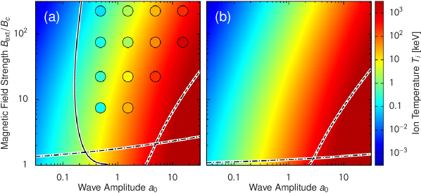
Figure 4: Dependence of the model prediction for the ion temperature on the initial parameters $a_{0}$, $B_{\rm ext}/B_{c}$, and $n_{e}/n_{c}$. (a) Predicted ion temperature given by Eq. (10) for the cases of $n_{e0}/n_{c}=19.3$. The wavelength is assumed to be $\lambda_{0}=0.8$ $\mu$m. Overplotted colored circles indicate $T_{i}$ obtained by the 1D PIC simulations with given parameters $a_{0}$ and $B_{\rm ext}/B_{c}$. In these runs, a flat-top pulse shape is used with a sufficiently long duration $\tau_{0}\gg\tau_{\rm sat}$. The valid range of the temperature prediction is within the area surrounded by three critical curves, which are obtained from the pressure-gradient condition [Eq. (14); solid curve] and the cyclotron resonance conditions [Eqs. (15) and (16); dashed and dot-dashed curves]. (b) Same diagram for the cases of $n_{e0}/n_{c}=10$ and $\lambda_{0}=1$ cm.

The force free condition, $E_{x}+(\bm{v}_{e}\bm{\times}\bm{B})_{x}\approx 0$, should be satisfied for the electron fluid, because the inertial and pressure-gradient terms in the electron equation of motion are negligible in the current situation ($\widetilde{n}_{e0}\gg 1$ and $T_{e}\sim 0$). The force balance for electrons is established distinctly in the PIC simulation [Fig. 3(a)]. The electromotive force acts as the negative ponderomotive force in this circumstance. The electrons gather periodically at the antinodes of the standing whistler waves to generate the longitudinal electric field $E_{x}$. The amplitude of $E_{x}$ is then evaluated as

$$E_{x}\approx-\left[\frac{8Na_{0}^{2}}{(N+1)^{2}(\widetilde{B}_{\rm ext}-1)}\frac{m_{e}c\omega_{0}}{e}\right]\sin(2Nk_{0}x)\;,$$ (5)

by using Eqs. (2) and (3), which has a sinusoidal distribution with the wavelength of $\lambda_{w}/2$. Interestingly, the electric field $E_{x}$ is constant in time, so that the ions are accelerated effectively by this tiny-scale steady force.

III.1 Ion temperature

The equation of motion for ions is approximately written as $\partial v_{xi}/\partial t\approx ZeE_{x}/m_{i}$, because of the slow velocity and low temperature initially ($v_{xi}\ll c$ and $T_{i}\sim 0$). Here $m_{i}$ and $Z$ are the ion mass and charge number, respectively. Since the electric force is independent of time, the amplitude of ion velocity increases linearly with time,

$$v_{xi}\approx\frac{ZeE_{x}}{m_{i}}(t-t_{s})\;,$$ (6)

where the displacement of the ion position is ignored, and $t_{s}$ is the time when the standing whistler wave appears in the target. As seen from Fig. 3(b), the constant acceleration of ion velocity is consistent with the PIC results from $\omega_{0}t\sim 120$ to 190. The ion density increases at the antinodes of the standing wave in the same manner as the electrons. Then the amplitude of the periodic density fluctuation of the electrons increases even further instantaneously to sustain the constant electric field $E_{x}$ as long as the standing waves survive. This positive feedback cycle continues to accelerate ions.

The ion acceleration will be terminated by the steepening of the waveform in the position-velocity phase diagram. Due to the huge density fluctuation caused by the localization of electrons and ions, the standing wave is no longer sustained and breaks down at the saturation time $\tau_{\rm sat}$ that is approximately estimated by

$$\int^{t_{s}+\tau_{\rm sat}}_{t_{s}}|v_{xi}|dt\sim\frac{\lambda_{w}}{8}\;,$$ (7)

where $\lambda_{w}/8$ corresponds to the acceleration length for the fastest ions, that is, a quarter of the ion wavelength [see Fig. 3(b)]. Solving this relation, the maximum amplitude is obtained as

$$\frac{v_{xi,\max}}{c}\sim\left[\frac{4\pi a_{0}^{2}}{(N+1)^{2}(\widetilde{B}_{\rm ext}-1)}\frac{Zm_{e}}{m_{i}}\right]^{1/2}\;,$$ (8)

at the time

$$\omega_{0}\tau_{\rm sat}\sim\left[\frac{\pi}{16}\frac{(N+1)^{2}(\widetilde{B}_{\rm ext}-1)}{N^{2}a_{0}^{2}}\frac{m_{i}}{Zm_{e}}\right]^{1/2}\;.$$ (9)

The solution suggests that the wave duration $\tau_{0}$ must be longer than $\tau_{\rm sat}$ in order for ions to gain the maximum energy from the standing whistler wave. The saturation time could be a few tens of the wave period or even shorter for the relativistic intensity cases $a_{0}\gtrsim 1$.

After the steepening, counter ion flows coexist at the same location, and the ions begin to thermalize through wave breaking and kinetic instabilities like ion two-stream instability Ross et al. (2013). If the accelerated ions are totally thermalized, it will give a reasonable evaluation of the maximum ion temperature, i.e.,

$$\frac{k_{B}T_{i}}{m_{e}c^{2}}\sim\frac{2\pi}{3}\frac{a_{0}^{2}Z}{(N+1)^{2}(\widetilde{B}_{\rm ext}-1)}\;,$$ (10)

where the relation $\langle v_{i}^{2}\rangle={3k_{B}T_{i}}/{m_{i}}\sim v_{xi,\max}^{2}/2$ is adopted. The PIC simulations confirm that the modeled temperature calculated from Eq. (10) is genuinely reliable to interpret the outcome of the counter CP light irradiation [see Fig. 4(a)]. According to the theoretical model, the final ion temperature is independent of the ion mass, but proportional to the charge $Z$. In the overdense limit, $\widetilde{n}_{e0}\gg\widetilde{B}_{\rm ext}>1$, the dependence of $T_{i}$ is proportional to $a_{0}^{2}Z/\widetilde{n}_{e0}$. During the collapsing regime, only ions are accelerated and heated selectively. That is why it can be regarded as a mechanism of direct ion-heating by electromagnetic waves. Note that the same phenomenon occurs by the left-hand CP lights if the plasma density is overdense and less than the L-cutoff, $1\lesssim\widetilde{n}_{e0}\lesssim\widetilde{n}_{L}\equiv\widetilde{B}_{\rm ext}+1$. The standing waves could be generated even with a single whistler wave by the reflection at the rear edge of a thin target.

III.2 Electron heating

The electron heating, on the other hand, would be dominated by the resistive heating at least in the 1D situation. The energy equation is given by

$$\frac{3}{2}\frac{\partial}{\partial t}(k_{B}T_{e})\approx m_{e}\nu_{ei}|\bm{v}_{e}-\bm{v}_{i}|^{2}\;,$$ (11)

where the relative velocity between electrons and ions is mainly caused by the quiver motion of whistler waves [Eq. (4)]. Assuming the Maxwellian-averaged collision frequency Kruer (2003); Chen (1984),

$$\nu_{ei}=\frac{\ln\Lambda}{3(2\pi)^{3/2}}\frac{Ze^{4}}{\varepsilon_{0}^{2}m_{e}^{1/2}}\frac{n_{e}}{(k_{B}T_{e})^{3/2}}\;,$$ (12)

the electron temperature is derived as

$$\frac{k_{B}T_{e}}{m_{e}c^{2}}\sim\left[\frac{40\sqrt{2\pi}\ln\Lambda}{9}\frac{a_{0}^{2}\widetilde{n}_{e0}}{(N+1)^{2}(\widetilde{B}_{\rm ext}-1)^{2}}\frac{Zr_{e}}{\lambda_{0}}\omega_{0}t\right]^{2/5}\;,$$ (13)

where $r_{e}={e^{2}}/({4\pi\varepsilon_{0}m_{e}c^{2}})$ is the electron classical radius. There is a wide parameter range where the ion temperature $T_{i}$ becomes higher than $T_{e}$.

In the PIC simulations, we neglect the initial temperature of the target. Even when the finite temperature is considered initially, the ion-heating process is found to be unchanged if the initial electron temperature is lower than the temperature given by Eq. (13).

III.3 Valid range of the model prediction

The ion temperature is now easily estimated from three initial parameters ($a_{0}$, $\widetilde{B}_{\rm ext}$, and $\widetilde{n}_{e0}$) with the help of Eq. (10). Figure 4(a) shows the predicted ion temperature for the cases of $\widetilde{n}_{e0}=19.3$ assuming a typical wavelength of high-intensity lasers $\lambda_{0}=0.8$ $\mu$m. Numerically obtained ion temperatures in the PIC simulations are overplotted by the colored circles, which show good agreement with the model prediction in a wide range from $T_{i}\sim 100$ eV to 1 MeV. The deviation from the model prediction is within a factor of 2 for the cases of $a_{0}\gtrsim 1$.

It should be noticed that there is a valid range of the theoretical model. One of the essential quantities of this heating mechanism is the longitudinal field $E_{x}$ given by Eq. (5). If the pressure-gradient term in the electron equation of motion is not negligible, the electromotive force could balance with $\nabla P_{e}$, and then the static electric field would not appear. Therefore, our model requires $\nabla P_{e}\sim 2k_{w}P_{e}\lesssim en_{e}(\bm{v}_{e}\bm{\times}\bm{B})_{x}$, which is rewritten by the initial parameters as

$$a_{0}\gtrsim\left[\frac{5\sqrt{2\pi}\ln\Lambda}{36}(N+1)^{3}(\widetilde{B}_{\rm ext}-1)^{1/2}\widetilde{n}_{e0}\frac{Zr_{e}}{\lambda_{0}}\omega_{0}t\right]^{1/3}\;,$$ (14)

where $\ln\Lambda$ is the Coulomb logarithm. This validity condition is shown by the solid curve in Fig. 4 assuming $\ln\Lambda=10$, $Z=1$, and $\omega_{0}t=300$. The pressure-gradient term is dominant for the lower intensity cases, because of the weaker dependence $\nabla P_{e}\propto T_{e}\propto a_{0}^{4/5}$ than $(\bm{v}_{e}\bm{\times}\bm{B})_{x}\propto a_{0}^{2}$.

Another requirement is to avoid the electron cyclotron resonance, which prevents whistler wave propagation by disturbing the electron quiver motion. The relativistic and Doppler effects must be considered to derive the resonance condition, $\omega_{0}-k_{w}v_{\parallel}=\omega_{ce}/\gamma$ Sano et al. (2017). Assuming $v_{\parallel}$ is of the order of the thermal velocity $v_{\rm th}$, the resonance condition is summarized as $\widetilde{B}_{\rm ext}\gtrsim\gamma$ and $\widetilde{B}_{\rm ext}\gtrsim 1+\widetilde{n}_{e0}^{1/3}(v_{\rm th}/c)^{2/3}$ in the relativistic and nonrelativistic limit, respectively. Here $\gamma\sim(1+a_{w}^{2})^{1/2}$ and $v_{\rm th}=(k_{B}T_{e}/m_{e})^{1/2}$ are the Lorentz factor and thermal velocity of electrons. By using the initial parameters, these conditions are settled in

$$a_{0}\lesssim\frac{(N+1)(\widetilde{B}_{\rm ext}^{2}-1)^{1/2}}{2}\;,$$ (15)

and

$$\widetilde{B}_{\rm ext}\gtrsim 1+\left[\frac{40\sqrt{2\pi}\ln\Lambda}{9}\frac{a_{0}^{2}\widetilde{n}_{e0}^{7/2}}{(N+1)^{2}}\frac{Zr_{e}}{\lambda_{0}}\omega_{0}t\right]^{2/19}\;,$$ (16)

which are also plotted by the dashed and dot-dashed curves in Fig. 4. In the end, the ion temperature given by Eq. (10) is applicable only within the area surrounded by these three curves.

IV Parameter dependence of ion energy increase

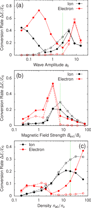
Figure 5: Parameter dependence of the energy conversion rate for ions and electrons obtained by 1D PIC simulations. (a) The conversion rate for ions (black) and electrons (red) as a function of the wave amplitude $a_{0}$. The conversion rate is evaluated at $\omega_{0}t_{\rm end}=2.78\times 10^{3}$. The filled and open circles denote the results with and without the Coulomb collision effects, respectively. The vertical dotted line indicates the fiducial parameter $a_{0}=2.65$. (b and c) Dependence on (b) the external field strength $B_{\rm ext}/B_{c}$ and (c) the plasma density of the target $n_{e0}/n_{c}$. The meanings of the marks are the same as in (a). The initial parameters are the same as in the fiducial run except for (b) $B_{\rm ext}$ and (c) $n_{e0}$. The fiducial parameters are $B_{\rm ext}/B_{c}=7.47$ and $n_{e0}/n_{c}=19.3$.

When the standing whistler wave heating sets in, the total ion energy is usually higher than the electron energy. Then the energy conversion rate will be a good indicator of the ion heating by standing whistler waves. Figure 5 shows the parameter dependence of the energy conversion rate for ions and electrons obtained from 1D PIC simulations similar to the fiducial run.

First, we investigate the effects of the incident wave amplitude. As seen from Fig. 5(a), where the initial parameters of these runs are identical to those in the fiducial run except for $a_{0}$, the ion energy is dominant when the wave amplitude is about $a_{0}\sim 1$–$5$. In other cases, the formation of standing waves is inhibited by higher electron temperature by the resistive heating or the cyclotron resonance. This is actually consistent with the validity conditions given by Eqs. (14) and (15).

The next parameter is the strength of the external magnetic field. As expected, the ion energy is dominant only when the magnetic field $B_{\rm ext}$ is sufficiently larger than the critical value $B_{c}$ [Fig. 5(b)]. The conversion efficiency decreases as the field strength increases so that the best condition for the ion heating is around $\widetilde{B}_{\rm ext}\sim$ 5–10.

As for the target density, obviously it must be overdense $\widetilde{n}_{e0}\gtrsim 2$ for efficient ion heating [Fig. 5(c)]. In the overdense limit, the electron temperature given by Eq. (13) is independent of the initial density $n_{e0}$, while the ion temperature has a dependence $T_{i}\propto n_{e0}^{-1}$. Then the energy fraction of electrons becomes predominant in this limit.

The wavelength of the incident CP lights is assumed to be $\lambda_{0}=0.8$ $\mu$m in our PIC simulations. The Coulomb collision term in the equation of motion for the charged particles has a dependence on the critical density. If the longer wavelength is selected, the relative importance of the collision effects becomes weaker. In Fig. 5, the results of collisionless simulations are also shown as a reference. When the collision effect is negligible, or the wave frequency is sufficiently high, the energy conversion to electrons is reduced significantly. Figure 4(b) indicates the ion temperature heated with the whistler wavelength of $\lambda_{0}=1$ cm assuming the target density $\widetilde{n}_{e0}=10$. The validity curves are largely different from those in the $\lambda_{0}=0.8$ $\mu$m cases. The pressure-gradient condition given by Eq. (14) is out of range in this figure ($a_{0}<0.01$). Therefore the standing whistler wave heating is realized in a broader range of the plasma parameters.

V Discussion and Conclusions

	Frequency (Wavelength)
	300 THz (1 $\mu$m)	30 THz (10 $\mu$m)	30 GHz (1 cm)	3 kHz (100 km)		Parameter	Range
Wave Amplitude (W/cm2)	$3\times 10^{18}$–$10^{20}$	$3\times 10^{16}$–$10^{18}$	$3\times 10^{10}$–$10^{12}$	$3\times 10^{-4}$–$10^{-2}$		$a_{0}$	$1$–$5$
Magnetic Field Strength (T)	$5\times 10^{4}$–$10^{5}$	$5\times 10^{3}$–$10^{4}$	$5$–$10$	$5\times 10^{-7}$–$10^{-6}$		$B_{\rm ext}/B_{c}$	$5$–$10$
Density (cm-3)	$2\times 10^{21}$–$10^{23}$	$2\times 10^{19}$–$10^{21}$	$2\times 10^{13}$–$10^{15}$	$0.2$–$10$		$n_{e0}/n_{c}$	$2$–$100$
Application	glass & TiSap laser	CO2 laser	tokamak	planetary magnetosphere

Table 1: Characteristic physical quantities for the thermal ion-plasma generation over 10 keV. The appropriate values of the wave amplitude, external magnetic field strength, and plasma density are listed for various cases of the frequency (wavelength) of electromagnetic waves. The range of each quantities in the non-dimensional parameter are also listed in the table.

The standing whistler wave heating is expected to develop various applications. For ICF, ions should be heated up to the higher temperature exceeding keV in imploded dense plasmas. Our method might give an advanced technique for an alternative ignition scheme of ICF by a completely different use of magnetic fields from the previous ideas Hohenberger et al. (2012); Perkins et al. (2013); Wang et al. (2015); Fujioka et al. (2016); Sakata et al. (2018). The keV ion plasma generated by this method could be an efficient thermal neutron source Baker et al. (2018). Since it requires the existence of a strong magnetic field larger than $B_{c}\approx 10$ kT for $\lambda_{0}=1$ $\mu$m, practically the generation of such an extreme magnetic field would be the first serious barrier to be resolved. Recently, the achievement of strong magnetic fields of kilo-Tesla order in laser experiments has been reported by several groups Yoneda et al. (2012); Fujioka et al. (2013); Goyon et al. (2017); Santos et al. (2018). Then it would be plausible in the near future to excite relativistic whistler waves from high-intensity lasers under a supercritical field condition $B_{\rm ext}>B_{c}$ Korneev et al. (2015).

The critical value $B_{c}$ can be reduced significantly by a choice of the longer wavelength. The typical quantities suitable for the standing whistler wave heating are summarized in Table 1. The carbon dioxide laser of the wavelength $\lambda_{0}=10$ $\mu$m might be a better choice for the proof-of-principle experiment of this mechanism, because the critical field strength decreases by an order of magnitude. If the wavelength is of the order of centimeter, the critical field strength goes down to $B_{c}\sim 1$ T. The situation shown in Figure 4(b) corresponds to a tokamak plasma of the density $n_{e0}=1.11\times 10^{14}$ cm^-3 ($\widetilde{n}_{e0}=10$) when the wavelength $\lambda_{0}=1$ cm is used. Based on the model prediction, the intensity $a_{0}\sim 0.5$ is needed to produce 10 keV ion plasma under a ITER-relevant magnetic field ($B_{\rm ext}\sim 5$ T) Stacey (2005). The other extreme case is $\lambda_{0}\sim 100$ km, or $\omega_{0}/(2\pi)\sim 3$ kHz, which gives $B_{c}\sim 100$ nT. These quantities are appropriate to the ion acceleration in planetary magnetospheres Bagenal (1992). It must be meaningful to pursue various applicability of this mechanism by a series of PIC simulations.

Ions and electrons are heated by the decay of whistler turbulence observed in the solar wind Alexandrova et al. (2013); Hughes et al. (2014); Gary et al. (2016). Interactions of counter-propagating waves should frequently occur in the turbulence so that it is interesting to examine the collisions of two waves with different frequencies. In this study, after the collapse of the standing whistler wave, the turbulent state of low-beta plasma is excited by ion kinetic instabilities and residual whistler waves. The gradual increase of the ion energy after the wave breaking [see Fig. 2(a)] might be caused by decaying whistler turbulence. Thus the multi-dimensional study of the turbulent stage would be applicable to the solar wind problem.

In summary, an ion-heating mechanism by the counter configuration of whistler waves has been investigated numerically and theoretically. The critical process is the collapse of standing whistler waves, which enables direct energy transfer from the electromagnetic waves to ions. The ion temperature is found to be estimated very accurately from three initial parameters that are the wave amplitude $a_{0}$, magnetic field strength $\widetilde{B}_{\rm ext}$, and plasma density $\widetilde{n}_{e0}$. Typical parameter ranges for thermal plasma generation over 10 keV are $a_{0}\sim$ 1–5, $\widetilde{B}_{\rm ext}\sim$ 5–10, and $\widetilde{n}_{e0}\sim$ 2–100. If a pair of linearly polarized lights are used instead of the counter CP lights, a part of the incident lights is converted to the whistler-mode and enters the overdense target Sano et al. (2017). Thus the same mechanism of ion heating takes place by the transmitted whistler waves, but the energy conversion efficiency is much lower than the CP cases.

Although we focus on 1D results in this paper, 2D PIC simulations, where the periodic boundary condition is imposed in another spatial direction $y$, reveals successfully that the same ion heating occurs in 2D as well (see Appendix). The only difference is observed in the higher electron temperature than the 1D counterpart when the width of the computational domain in the $y$ direction becomes comparable to the whistler wavelength. The detailed analysis in multi-dimensional cases will be an essential subject for our future work.

*

Appendix A Two-dimensional effects

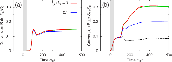
Figure 6: Time evolution of energy conversion rate for (a) ions and (b) electrons is depicted for various cases of $L_{y}/\lambda_{0}=3$ (red), 1 (green), and 0.1 (blue) of the 2D runs. The initial parameters are the same as in the 1D fiducial run except for the target thickness $L_{x}/\lambda_{0}=18.75$ and the pulse duration $\omega_{0}\tau_{0}=35.3$. The dashed curve is the result of the 1D run, that is, $L_{y}=0$.

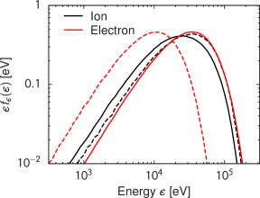
Figure 7: Energy spectrum $\epsilon f_{\epsilon}(\epsilon)$ of ions (black) and electrons (red) at the end of the calculation $\omega_{0}t_{\rm end}=1.84\times 10^{3}$ are plotted for the cases of $L_{y}/\lambda_{0}=3$ (solid) and 0 (bashed). These spectra are calculated from the particles located at the standing wave region $|x/\lambda_{0}|\leq 5$.

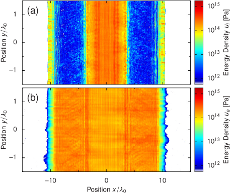
Figure 8: Spatial distributions of the energy density $u$ for (a) ions and (b) electrons in a 2D simulation. The energy density is measured in the unit of Pascal. The initial parameters are the same as in the 1D fiducial run except for the target thickness $L_{x}/\lambda_{0}=18.75$ and the pulse duration $\omega_{0}\tau_{0}=35.3$. The box size in the $y$ direction is $L_{y}/\lambda_{0}=3$. These images are taken at $\omega_{0}t=329$.

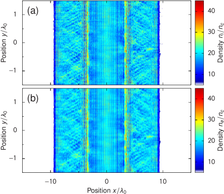
Figure 9: Spatial distribution of the density $n$ for (a) ions and (b) electrons in the 2D run. The initial parameters and snapshot timing are the same as those in the 2D run shown by Fig 9.

The ion-heating mechanism by standing whistler waves is observed in 2D PIC simulations, which are performed to compare with the 1D behavior. The initial parameters are the same as in the 1D fiducial run except for the target thickness $L_{x}/\lambda_{0}=18.75$ and the pulse duration $\omega_{0}\tau_{0}=35.3$. The resolution in 2D runs is $\Delta x=c\Delta t=\lambda_{0}/300$ and the particle number per cell is 60. The computational box size of the additional spatial direction $y$ is considered from $L_{y}/\lambda_{0}=0.1$ to 3. In the $y$ direction, the wave injection from the boundaries is uniform, and the periodic boundary condition is adopted.

Dependence of the energy conversion rate on the domain size in the $y$ direction is shown in Fig. 6. Obviously the ion evolution is independent of $L_{y}/\lambda_{0}$. The electron energy increases when $L_{y}/\lambda_{0}$ becomes comparable to the whistler wavelength, which is $\lambda_{w}/\lambda_{0}\sim 0.5$ for the fiducial parameters. However, it seems to be saturated if $L_{y}\gg\lambda_{w}$. The same trend is recognized in the comparison of the energy spectra between 1D and 2D simulations (Fig. 7). All the spectra are well fitted by the thermal distribution of a single temperature. The ion temperature estimated by the Maxwellian fitting is 22 keV for the 1D run and 18 keV for 2D so that the ion spectra are unaffected by 2D effects. The electron spectrum in 2D exhibits higher energy than that in 1D. The electron temperature is 7.2 and 23 keV for 1D and 2D runs, respectively.

The ion energy is enhanced only at the central part of the target, $|x/\lambda_{0}|\lesssim 5$, where a standing whistler wave is formed. Figure 8 shows the spatial distributions of the energy density $u$ for ions and electrons in a 2D simulation with $L_{y}/\lambda_{0}=3$. It looks almost 1D-like distribution, and thus the ion evolution is quite similar to the 1D case. On the other hand, the electron energy is nearly uniform after the passage of the injected whistler waves. Because of the transverse propagation of the electron plasma waves, the electrons absorb a larger amount of energy from the waves compared with the corresponding 1D result. The evidence of the transverse plasma waves is observed in the spatial distribution of density fluctuations during the standing whistler wave heating (Fig. 9). The initial parameters and the snapshot timing are the same as in Fig. 8. The standing whistler wave causes vertical stripes in the middle part. Small-scale fluctuations of the order of the whistler wavelength are seen in the transverse direction.

References

- Kruer (2003) W. L. Kruer, The Physics of Laser Plasma Interactions (Westview Press, Boulder, 2003).
- Lembege et al. (2004) B. Lembege, J. Giacalone, M. Scholer, T. Hada, M. Hoshino, V. Krasnoselskikh, H. Kucharek, P. Savoini, and T. Terasawa, Space Sci. Rev. 110, 161 (2004).
- Stenzel (1999) R. L. Stenzel, J. Geophys. Res. 104, 14379 (1999).
- Stenzel (2016) R. L. Stenzel, Adv. Phys. X 1, 687 (2016).
- Lindl (1995) J. Lindl, Phys. Plasmas 2, 3933 (1995).
- Betti and Hurricane (2016) R. Betti and O. A. Hurricane, Nat. Phys. 12, 435 (2016).
- Stacey (2005) W. M. Stacey, Fusion Plasma Physics (Wiley-VCH, Weinheim, 2005).
- Helliwell (1965) R. A. Helliwell, Whistlers and Related Ionospheric Phenomena (Stanford University Press, Stanford, 1965).
- Tsurutani and Smith (1974) B. T. Tsurutani and E. J. Smith, J. Geophys. Res. 79, 118 (1974).
- Coroniti et al. (1980) F. V. Coroniti, F. L. Scarf, C. F. Kennel, W. S. Kurth, and D. A. Gurnett, Geophys. Res. Lett. 7, 45 (1980).
- Hospodarsky et al. (2008) G. B. Hospodarsky, T. F. Averkamp, W. S. Kurth, D. A. Gurnett, J. D. Menietti, O. Santolik, and M. K. Dougherty, J. Geophys. Res. 113, n/a (2008).
- Artemyev et al. (2016) A. Artemyev, O. Agapitov, D. Mourenas, V. Krasnoselskikh, V. Shastun, and F. Mozer, Space Sci. Rev. 200, 261 (2016).
- Horne et al. (2005) R. B. Horne, R. M. Thorne, S. A. Glauert, J. M. Albert, N. P. Meredith, and R. R. Anderson, J. Geophys. Res. 110, A03225 (2005).
- Omura et al. (2007) Y. Omura, N. Furuya, and D. Summers, J. Geophys. Res. 112, A06236 (2007).
- Summers and Omura (2007) D. Summers and Y. Omura, Geophys. Res. Lett. 34, L24205 (2007).
- Thorne et al. (2013) R. M. Thorne, W. Li, B. Ni, Q. Ma, J. Bortnik, L. Chen, D. N. Baker, H. E. Spence, G. D. Reeves, M. G. Henderson, C. A. Kletzing, W. S. Kurth, G. B. Hospodarsky, J. B. Blake, J. F. Fennell, S. G. Claudepierre, and S. G. Kanekal, Nature 504, 411 (2013).
- Prater et al. (2014) R. Prater, C. Moeller, R. Pinsker, M. Porkolab, O. Meneghini, and V. Vdovin, Nucl. Fusion 54, 083024 (2014).
- Mourenas (1998) D. Mourenas, Phys. Plasmas 5, 243 (1998).
- Taguchi et al. (2017) T. Taguchi, T. M. Antonsen, and K. Mima, J. Plasma Phys. 83, 905830204 (2017).
- Yang et al. (2015) X. H. Yang, W. Yu, H. Xu, M. Y. Yu, Z. Y. Ge, B. B. Xu, H. B. Zhuo, Y. Y. Ma, F. Q. Shao, and M. Borghesi, Appl. Phys. Lett. 106, 224103 (2015).
- Ma et al. (2016) G. Ma, W. Yu, M. Y. Yu, S. Luan, and D. Wu, Phys. Rev. E 93, 053209 (2016).
- Weng et al. (2017) S. Weng, Q. Zhao, Z. Sheng, W. Yu, S. Luan, M. Chen, L. Yu, M. Murakami, W. B. Mori, and J. Zhang, Optica 4, 1086 (2017).
- Sano et al. (2017) T. Sano, Y. Tanaka, N. Iwata, M. Hata, K. Mima, M. Murakami, and Y. Sentoku, Phys. Rev. E 96, 043209 (2017).
- Nishikawa (1968) K. Nishikawa, J. Phys. Soc. Japan 24, 916 (1968).
- Forslund et al. (1972) D. W. Forslund, J. M. Kindel, and E. L. Lindman, Phys. Rev. Lett. 29, 249 (1972).
- Lee (1974) K. F. Lee, Phys. Fluids 17, 1343 (1974).
- Hsu et al. (1979) J. Y. Hsu, K. Matsuda, M. S. Chu, and T. H. Jensen, Phys. Rev. Lett. 43, 203 (1979).
- Doveil (1981) F. Doveil, Phys. Rev. Lett. 46, 532 (1981).
- Tran (1982) M. Q. Tran, IEEE Trans. Plasma Sci. 10, 16 (1982).
- Luan et al. (2016) S. X. Luan, W. Yu, F. Y. Li, D. Wu, Z. M. Sheng, M. Y. Yu, and J. Zhang, Phys. Rev. E 94, 053207 (2016).
- Sentoku and Kemp (2008) Y. Sentoku and A. J. Kemp, J. Comp. Phys. 227, 6846 (2008).
- Ross et al. (2013) J. S. Ross, H.-S. Park, R. Berger, L. Divol, N. L. Kugland, W. Rozmus, D. Ryutov, and S. H. Glenzer, Phys. Rev. Lett. 110, 145005 (2013).
- Chen (1984) F. F. Chen, Introduction to Plasma Physics and Controlled Fusion (Plenum Press, New York, 1984).
- Hohenberger et al. (2012) M. Hohenberger, P.-Y. Chang, G. Fiksel, J. P. Knauer, R. Betti, F. J. Marshall, D. D. Meyerhofer, F. H. Séguin, and R. D. Petrasso, Phys. Plasmas 19, 056306 (2012).
- Perkins et al. (2013) L. J. Perkins, B. G. Logan, G. B. Zimmerman, and C. J. Werner, Phys. Plasmas 20, 072708 (2013).
- Wang et al. (2015) W.-M. Wang, P. Gibbon, Z.-M. Sheng, and Y.-T. Li, Phys. Rev. Lett. 114, 015001 (2015).
- Fujioka et al. (2016) S. Fujioka, Y. Arikawa, S. Kojima, T. Johzaki, H. Nagatomo, H. Sawada, S. H. Lee, T. Shiroto, N. Ohnishi, A. Morace, X. Vaisseau, S. Sakata, Y. Abe, K. Matsuo, K. F. F. Law, S. Tosaki, A. Yogo, K. Shigemori, Y. Hironaka, Z. Zhang, A. Sunahara, T. Ozaki, H. Sakagami, K. Mima, Y. Fujimoto, K. Yamanoi, T. Norimatsu, S. Tokita, Y. Nakata, J. Kawanaka, T. Jitsuno, N. Miyanaga, M. Nakai, H. Nishimura, H. Shiraga, K. Kondo, M. Bailly-Grandvaux, C. Bellei, J. J. Santos, and H. Azechi, Phys. Plasmas 23, 056308 (2016).
- Sakata et al. (2018) S. Sakata, S. Lee, H. Morita, T. Johzaki, H. Sawada, Y. Iwasa, K. Matsuo, K. F. F. Law, A. Yao, M. Hata, A. Sunahara, S. Kojima, Y. Abe, H. Kishimoto, A. Syuhada, T. Shiroto, A. Morace, A. Yogo, N. Iwata, M. Nakai, H. Sakagami, T. Ozaki, K. Yamanoi, T. Norimatsu, Y. Nakata, S. Tokita, N. Miyanaga, J. Kawanaka, H. Shiraga, K. Mima, H. Nishimura, M. Bailly-Grandvaux, J. J. Santos, H. Nagatomo, H. Azechi, R. Kodama, Y. Arikawa, Y. Sentoku, and S. Fujioka, Nat. Comm. 9, 3937 (2018).
- Baker et al. (2018) K. L. Baker, C. A. Thomas, D. T. Casey, S. Khan, B. K. Spears, R. Nora, T. Woods, J. L. Milovich, R. L. Berger, D. Strozzi, D. Clark, M. Hohenberger, O. A. Hurricane, D. A. Callahan, O. L. Landen, B. Bachmann, R. Benedetti, R. Bionta, P. M. Celliers, D. Fittinghoff, C. Goyon, G. Grim, R. Hatarik, N. Izumi, M. Gatu Johnson, G. Kyrala, T. Ma, M. Millot, S. R. Nagel, A. Pak, P. K. Patel, D. Turnbull, P. L. Volegov, and C. Yeamans, Phys. Rev. Lett. 121, 135001 (2018).
- Yoneda et al. (2012) H. Yoneda, T. Namiki, A. Nishida, R. Kodama, Y. Sakawa, Y. Kuramitsu, T. Morita, K. Nishio, and T. Ide, Phys. Rev. Lett. 109, 125004 (2012).
- Fujioka et al. (2013) S. Fujioka, Z. Zhang, K. Ishihara, K. Shigemori, Y. Hironaka, T. Johzaki, A. Sunahara, N. Yamamoto, H. Nakashima, T. Watanabe, H. Shiraga, H. Nishimura, and H. Azechi, Sci. Rep. 3, 1170 (2013).
- Goyon et al. (2017) C. Goyon, B. B. Pollock, D. P. Turnbull, A. Hazi, L. Divol, W. A. Farmer, D. Haberberger, J. Javedani, A. J. Johnson, A. Kemp, M. C. Levy, B. Grant Logan, D. A. Mariscal, O. L. Landen, S. Patankar, J. S. Ross, A. M. Rubenchik, G. F. Swadling, G. J. Williams, S. Fujioka, K. F. F. Law, and J. D. Moody, Phys. Rev. E 95, 033208 (2017).
- Santos et al. (2018) J. J. Santos, M. Bailly-Grandvaux, M. Ehret, A. V. Arefiev, D. Batani, F. N. Beg, A. Calisti, S. Ferri, R. Florido, P. Forestier-Colleoni, S. Fujioka, M. A. Gigosos, L. Giuffrida, L. Gremillet, J. J. Honrubia, S. Kojima, P. Korneev, K. F. F. Law, J.-R. Marquès, A. Morace, C. Mossé, O. Peyrusse, S. Rose, M. Roth, S. Sakata, G. Schaumann, F. Suzuki-Vidal, V. T. Tikhonchuk, T. Toncian, N. Woolsey, and Z. Zhang, Phys. Plasmas 25, 056705 (2018).
- Korneev et al. (2015) P. Korneev, E. d’Humières, and V. Tikhonchuk, Phys. Rev. E 91, 043107 (2015).
- Bagenal (1992) F. Bagenal, Annu. Rev. Earth Planet. Sci. 20, 289 (1992).
- Alexandrova et al. (2013) O. Alexandrova, C. H. K. Chen, L. Sorriso-Valvo, T. S. Horbury, and S. D. Bale, Space Sci. Rev. 178, 101 (2013), 1306.5336 .
- Hughes et al. (2014) R. S. Hughes, S. P. Gary, and J. Wang, Geophys. Res. Lett. 41, 8681 (2014).
- Gary et al. (2016) S. P. Gary, R. S. Hughes, and J. Wang, Astrophys. J. 816, 102 (2016).