Pre-discovery Activity of New Interstellar Comet 2I/Borisov Beyond 5 AU
Abstract
Comet 2I/Borisov, the first unambiguous interstellar comet ever found, was discovered in August 2019 at au from the Sun on its inbound leg. No pre-discovery detection beyond 3 au has yet been reported, mostly due to the comet’s proximity to the Sun as seen from the Earth. Here we present a search for pre-discovery detections of comet Borisov using images taken by the Catalina Sky Survey (CSS), Pan-STARRS and Zwicky Transient Facility (ZTF), with a further comprehensive follow-up campaign being presented in Bolin et al. (2019). We identified comet Borisov in ZTF images taken in May 2019 and use these data to update its orbit. This allowed us to identify the comet in images acquired as far back as December 2018, when it was 7.8 au from the Sun. The comet was not detected in November 2018 when it was 8.6 au from the Sun, possibly implying an onset of activity around this time. This suggests that the activity of the comet is either driven by a more volatile species other than H2O, such as CO or CO2, or by exothermic crystallization of amorphous ice. We derive the radius of the nucleus to be km using the non-detection in November 2018, and estimate an area of — has been active between December 2018 and September 2019, though this number is model-dependent and is highly uncertain. The behavior of comet Borisov during its inbound leg is observationally consistent with dynamically new comets observed in our solar system, suggesting some similarities between the two.
1 Introduction
Comet 2I/Borisov111Formerly designated as C/2019 Q4 (Borisov). See Minor Planet Electronic Circular (MPEC) 2019-R106 and MPEC 2019-S72. (2I for short), discovered by G. Borisov at the Crimean Astrophysical Observatory on 2019 August 30, is the second interstellar object and the first unambiguous interstellar comet ever found. Early observations of 2I have revealed a sizeable coma (de León et al., 2019; Guzik et al., 2019; Jewitt & Luu, 2019) and the detection of the emission from CN and atomic oxygen (Fitzsimmons et al., 2019; Opitom et al., 2019; McKay et al., 2019). This makes it distinctively different from the first discovered interstellar object 1I/‘Oumuamua, which did not exhibit a detectable cometary feature such as a coma and/or a tail (Meech et al., 2017; Ye et al., 2017; ‘Oumuamua ISSI Team et al., 2019). The detection of activity is important as it provides a way to probe the composition of the nucleus, which can be done through a direct analysis of gases in the coma, and by observing how the activity responds to different levels of insolation at different heliocentric distances.
2I was discovered at a heliocentric distance au, with a brightness ( mag) that is well within the reach of modern near-Earth object (NEO) surveys. The belated discovery is primarily due to the fact that the comet was within from the Sun, within the typical solar avoidance zone for ground-based optical telescopes, from early May to early September 2019.
A detection (or non-detection) at au would better constrain the size of the nucleus (as the comet is likely less active) as well as its inbound orbit, and would be diagnostic of the comet’s volatile composition (Fitzsimmons et al., 2019), since the activity of most known (i.e., solar system) comets within –5 au is driven by water ice sublimation (e.g., Meech & Svoren, 2004). All-sky, time-domain surveys allow for serendipitous observations of objects before they are discovered. Here we present a search for pre-discovery detections of 2I in the data of several sky surveys. We will describe the search process in § 2, the procedure of photometric analysis in § 3, and will then discuss the implication of the detections and non-detections in § 4 and § 5.
2 Pre-discovery Detections
2.1 Zwicky Transient Facility
The Zwicky Transient Facility (ZTF) is a wide-field optical survey utilizing the 1.2 m Palomar Oschin Schmidt and a dedicated camera with 55 deg2 field-of-view (Bellm et al., 2019; Graham et al., 2019; Masci et al., 2019). Apart from two baseline surveys and a number of mini-surveys, ZTF executes a mini-survey (“Twilight Survey”) that observes regions with solar elongation down to (Ye et al., 2019), which is particularly suitable for the search of pre-discovery detections of 2I. The first phase of the ZTF Twilight Survey was executed from November 2018 to June 2019, fortuitously covering the period before 2I reached solar conjunction in July 2019.
By using the ZChecker comet monitoring package (Kelley et al., 2019) and JPL orbit solution #12 (the most recent JPL solution at the time that the search was conducted), we identified a total of 202 images from 2018 October 1 to the discovery date of 2I (2019 August 30) that potentially contained the comet. All images use 30 s exposure times, and were taken in a wide range of observing circumstances, with limiting magnitudes between 16–21 and seeing between –. The comet reached solar conjunction in July of 2019, and the last three sets of images acquired before that were taken in the course of the Twilight Survey on 2019 April 29, May 2 and May 5 respectively, when 2I was at –5.09 au. Prior to these Twilight Survey data, the last image was taken on 2019 April 16, when the comet was at au. The April 29 and May 5 observations were not optimal because only a few images were acquired, high sky background, and/or the comet being near image edges. The May 2 observations were particularly fortuitous as the comet was located in an overlapping strip between two fields, and thus have more images than we typically have (8 images total, instead of the typical 4 images per field). Therefore, we focused on the 2019 May 2 data for our initial search of a pre-discovery detection.
The astrometric observations available up to this point did not provide meaningful constraints on the cometary non-gravitational perturbations (e.g., Yeomans et al., 2004), which lead to different orbit solutions. To capture the ephemeris variations using different model assumptions, we fit the available astrometry as of 2019 October 3 using a gravity-only model, and two non-gravitational models that either assumed sublimation of H2O (Marsden et al., 1973) or CO (with sublimation rate )222To our best knowledge, the only CO-driven non-gravitational model published to-date is the Yabushita (1996) model. However, their elbow at au is inconsistent with both theoretical and observational results, which suggests an elbow of au (e.g. Biver et al., 1996; Gunnarsson et al., 2002; Meech & Svoren, 2004, Hui et al. in prep). Here we simply assume the sublimation rate follows , since the elbow is likely much larger than the largest in our dataset. to be the primary driver of comet activity. We then combined all 8 images from May 2 following the apparent motion of 2I. The three solutions are tabulated in Table 1 (together with the final orbit, after we have successfully identified the comet in the ZTF pre-discovery data, as we discuss below), and the combined image as well as the uncertainty ellipses of the three solutions are shown as Figure 1. Because of the short arc and the low elongation of many of the astrometric positions, we note that the estimated non-gravitational parameters could be unreliable. In particular, the parameters for the H2O-driven model appear to be too large to be credible, and are possibly caused by astrometric biases at such a small solar elongation.
| Parameter | Gravity-only | Nongrav – H2O | Nongrav – CO | Final – CO |
|---|---|---|---|---|
| (without precovery) | (without precovery) | (without precovery) | (with precovery) | |
| Epoch (TDB) | 2019 Sep 16.0 | 2019 Sep 16.0 | 2019 Sep 16.0 | 2019 Dec 20.0 |
| Perihelion time (TDB) | 2019 Dec 8.65 0.07 d | 2019 Dec 13 1 d | 2019 Dec 9.1 0.4 d | 2019 Dec 8.551 0.001 d |
| Perihelion distance (au) | ||||
| Eccentricity | ||||
| Inclination | ||||
| Long. Ascending Node | ||||
| Argument of Perihelion | ||||
| Radial accel. () | - | |||
| Transverse accel. () | - |
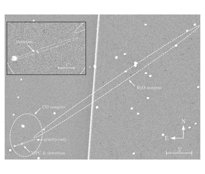
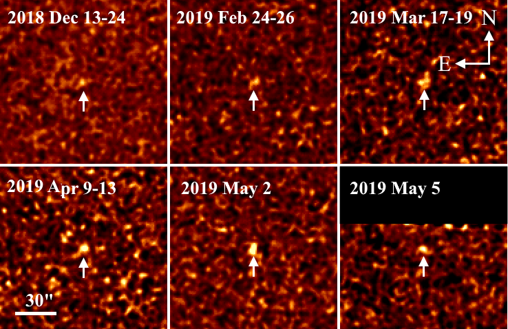
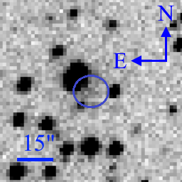
We identified a possible detection at a signal-to-noise ratio () of on the combined May 2 image (Figure 2). The detection is within the uncertainty ellipses of gravity-only and CO non-gravitational solutions, and about southeast of the predicted Minor Planet Center (MPC) position. Visually, the object is about in diameter and is largely circular in shape, with no apparent sign of a tail. The object is barely visible on individual frames (Figure 2), with a motion consistent with that of 2I.
We then examined other images in the time period in question, using the same shift-and-stack technique as outlined above. The detection on 2019 May 2, if real, would have greatly reduced the ephemeris uncertainty from a few arcminutes to a few arcseconds back to January 2019, and would enable more pre-discovery data to be found. Since the comet is extremely faint, in order to eliminate contamination due to variable sky conditions and passing background stars, we only use frames that have (1) limit of , (2) average full-width-half-maximum (FWHM) of pixels, and (3) have no background stars that are within from the predicted position of the comet.
All the pre-discovery detections and non-detections are summarized in Table 2. We were able to trace the object back to 2018 December 13. Apart from the 2019 May 2 data, the object is not visible in individual frames, and a clear detection usually requires stacking images from multiple nights. By including these astrometric positions333Published in MPEC 2019-V34 and MPEC 2019-W50. with the post-discovery astrometric measurements of 2I and considering the non-gravitational effect, we were able to get a satisfactory orbital fit with residuals of order , which is slightly above the average compared to typical ZTF astrometry (better than ). This is due to a weak systematic bias in the data, which is possibly caused by the fact that most astrometric data were taken at low solar elongation and therefore at high airmass, introducing some differential color refraction (DCR) bias (see also the discussion in § 4.4). Nevertheless, we identify the object observed from 2018 December 13 to 2019 May 5 as 2I.
| Images date | Median date (UT) | Survey | (au) | (au) | Images used | FWHM | Res. | mag |
|---|---|---|---|---|---|---|---|---|
| 2018 Oct 31 – 2018 Nov 21 | 2018 Nov 8.82 | ZTF | 8.55 | 7.90 | : 12; : 16 | – | - | |
| 2018 Dec 13 – 2018 Dec 22 | 2018 Dec 19.15 | ZTF | 7.75 | 6.99 | : 6; : 6 | – | ||
| 2019 Jan 17 | 2019 Jan 17.30 | PS1 | 7.18 | 6.58 | : 4 | – | - | - |
| 2019 Feb 24 – 2019 Feb 26 | 2019 Feb 25.18 | ZTF | 6.42 | 6.26 | : 3; : 4 | – | ||
| 2019 Mar 1 | 2019 Mar. 1.10 | CSS | 6.35 | 6.24 | Clear: 4 | |||
| 2019 Mar 16 – 2019 Mar 18 | 2019 Mar 17.18 | ZTF | 6.02 | 6.14 | : 4; : 5 | – | ||
| 2019 Apr 9 – 2019 Apr 13 | 2019 Apr 12.16 | ZTF | 5.53 | 5.97 | : 3; : 3 | – | ||
| 2019 May 2 | 2019 May 2.16 | ZTF | 5.15 | 5.79 | : 8 | – | ||
| 2019 May 5 | 2019 May 5.15 | ZTF | 5.09 | 5.76 | : 4 | – |
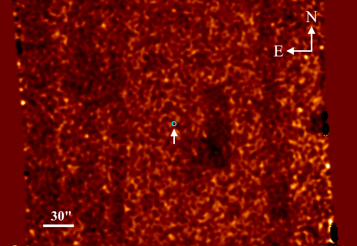
A point worth addressing is the non-detection in November 2018. The uncertainty of the position is (4 pixels) along the major axis, and the motion rate difference between different orbit solutions is less than 1/4th of a pixel over the entire time span, but no comet is detected in the stack (Figure 3). Subsequent light-curve analysis (see § 4.1) shows that 2I should be mag above than the limit of the stack.
2.2 Pan-STARRS
The Pan-STARRS survey (Chambers et al., 2016) is a wide-field asteroid survey comprised of two identical 1.8 m telescopes, the Pan-STARRS1 (PS1) and Pan-STARRS2 (PS2). The survey has an image archive extending back to 2010. Using the ZTF precovery data along with the available astrometry from the Minor Planet Center up to 2019 October 1, we generate an ephemeris covering the period from 2018 January 1 (when 2I was well below any practical ground based telescope sensitivity) until the discovery date of 2019 August 30. Four 45 second -band images taken by the PS1 system on 2019 January 17 were identified, as summarized in Table 2. The normal processing for Pan-STARRS applies masking to remove areas not optimal for photometry because of non-uniform charge transfer efficiency, and for this study, the exposures were reprocessed without this mask. They were then visually inspected carefully over a large region centered at the expected ephemeris. The predicted ephemeris and uncertainty, however, place 2I firmly into a -wide chip gap (Figure 4).
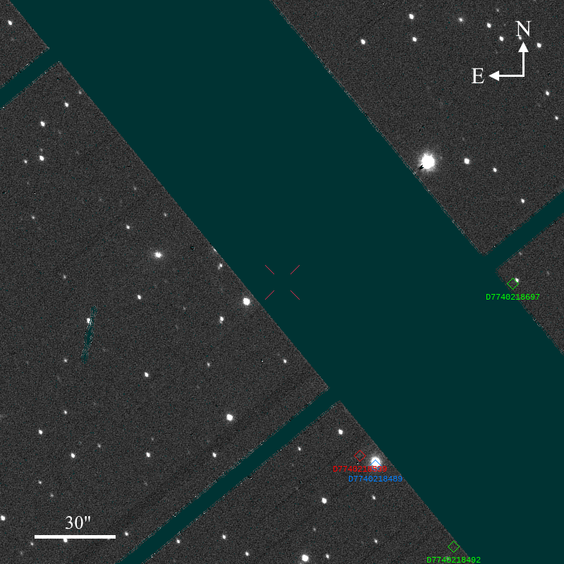
While no detections were found in the Pan-STARRS pre-discovery images, the fact that the expected location of 2I is contained within a chip gap favors the ZTF precovery positions being correct, as even a weakly active comet should have been visible otherwise given the limiting magnitude and near arcsecond seeing. The chip gap only occupies a small fraction ( based on the astrometry up to 2019 October 1) of the uncertainty ellipse, therefore there was a much larger chance of being proven wrong.
However, we note that PS1 was not operational between 2018 August 23 and December 12 due to a dome shutter failure, and between 2019 February 10 and March 27 due to loss of power after a winter storm on Haleakala where the telescope is installed.
2.3 Catalina Sky Survey
The Catalina Sky Survey (CSS; e.g. Christensen et al., 2018) operates three telescopes dedicated to the discovery and follow-up of near-Earth objects: the 0.7 m Catalina Schmidt at Mt. Bigelow, a 1.0 m telescope and a 1.5 m telescope at Mt. Lemmon, Arizona.
Following a similar strategy of the Pan-STARRS data search, we searched the archival data of all three telescopes dating back to 2018 January 1. We identified various sets of images covering the predicted ephemeris of 2I: multiple sets of images taken by the 0.7 m Catalina Schmidt, but all dated no later than 2018 December 15, and a set of four images taken by the 1.5 m telescope on 2019 March 1.
The comet was too faint ( mag beyond the limit of the image) for the December 2018 and earlier images, while the March 2019 images reached a limiting magnitude that could be compatible with a faint detection of 2I. However, the position corresponding to the ZTF detections fell on a region heavily contaminated with background field sources. In three of the four frames, the object would have overlapped the PSF of a field star. The remaining frame was also marginally affected by an even brighter nearby star, but it might show a slight enhancement that is within 1.5–2 pixels from the predicted position of 2I (Figure 5). A deeper stack of historical images obtained by Catalina with the same telescope reveals no background source at that position, down to a limiting magnitude much fainter than the individual frame. Unfortunately, the enhancement was extremely faint, and might be compatible with a noise feature enhanced by the tails of the bright star’s point-source-function (PSF), making it difficult to draw a solid conclusion.
3 Photometric Analysis
To measure the flux from 2I for each epoch specified in the 2nd column of Table 2, we scale each frame in the time range listed in the 1st column of the table with respect to a “reference” frame in this range using the following formula for frame combination:
| (1) |
where is the scale coefficient; and is the geocentric distance of the comet in the given frame and the reference frame, respectively; and is the heliocentric distance of the comet in the given frame and the reference frame, respectively444The exponent terms of and come from the classic comet brightness formula, , where and are the apparent and absolute total magnitude of the comet, and the flux of the comet is proportional to and , respectively. If we leave out these two terms, the non-detection photometry will differ by 0.5 mag compared to the values listed in Table 2. For other pre-discovery data points, the differences are within 0.05 mag. and the corrected magnitude zero-point is defined by
| (2) |
where is the magnitude zero-point and is the color coefficient derived by the ZTF Science Data System and calibrated to the PS1 photometric system (Masci et al., 2019), and is the color of the comet. We use as measured by Guzik et al. (2019), with the colors converted using the relations derived in Tonry et al. (2012). We use a fixed photometric aperture with a radius of 5 pixels, or 21000–29000 km at the comet in the interval of November 2018 and May 2019. This aperture is sufficient to include all flux from the comet in the pre-discovery data. The result is tabulated in Table 2.
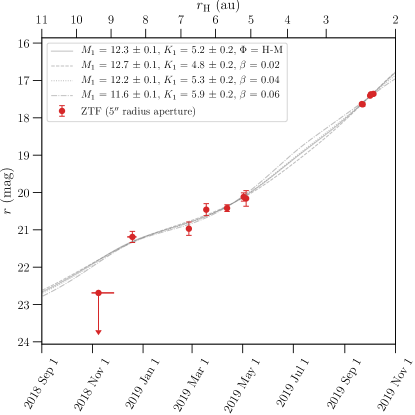
We then fit the light-curve using the classic comet light-curve equation:
| (3) |
where and are the apparent and absolute total magnitude of the comet, respectively, is the logarithmic heliocentric distance slope, and is the phase function of the comet with respect to the phase angle . We note that this process should not be confused with the image scaling process with Equation 1 as described above, as the purpose of the image scaling process was to scale a subset of data to a reference epoch (defined in the 2nd column of Table 2), while the photometry of each reference epoch is then used for the light-curve fitting described here.
We test four phase functions: the Marcus (2007) model on Halley’s Comet, as well as linear phase functions where , 0.04, and 0.06 mag deg-1 is the phase coefficient of the comet (Lamy et al., 2004). All four models yield comparable results, with varies from to , and from to , as shown in Figure 6.
4 Discussion
4.1 Driver of the Activity
The best-fit light-curve as shown in Figure 6 revealed a shallow slope, , taking a linear phase coefficient mag deg-1. A shallow slope means that the activity stays largely constant as the comet approaches the Sun. Whipple (1978) shows that shallow brightening is common on the “dynamically new” solar system comets (with orbital periods yr) which have ), but uncommon on short-period comets and other long-period comets, which have , though his dataset is dominated by small heliocentric distances with au. In this respect, 2I is analogous to dynamically new comets in the solar system.
The slope seemingly deviates from the data beyond au, preceded by what appears like a steep brightening phase, with , though additional pre-discovery observations are needed to verify it. If such steep phase is real, it might indicate the onset of sublimation of cometary volatiles. The most compatible major volatile would be CO2, which has an onset “knee” distance au. Other cometary species, such as CH3CN, HCN and CH3OH, have similar turn-on distances (Meech & Svoren, 2004), but they have low abundances in solar system comets (Cochran et al., 2015). CO, another cometary volatile commonly found on dynamically new comets in solar system that has an onset distance au, is not as compatible. However, it has been suggested for the case of ‘Oumuamua that the volatiles may be buried beneath the surface and are only activated when the comet is much closer to the Sun, due to the time lag for the heat wave to penetrate to the depth of the ice (Fitzsimmons et al., 2018; Seligman & Laughlin, 2018). Therefore, it is too early to exclude CO as the main driver of 2I’s activity.
An alternative explanation of the activity is the exothermic crystallization of amorphous water ice, a mechanism that may be responsible for the activity of distant comets (Prialnik & Bar-Nun, 1990). Amorphous ice forms below an environmental temperature of K and is capable of trapping gas as they form, a phenomenon that has been observed in laboratory experiments (Bar-Nun et al., 1987; Jenniskens & Blake, 1994), though the presence of amorphous ice is yet to be directly observed on comets. Depending on the illumination of the cometary nucleus, crystallization of amorphous ice on the surface can start around – au (Jewitt et al., 2017), consistent with the observed turn-on distance of 2I.
To gain a deeper insight into the light-curve, we tested a sublimation model (Meech & Svoren, 2004) that computes the amount of gas sublimating from an icy surface exposed to solar heating to explore the activity. The total brightness within a fixed aperture combines radiation scattered from both the nucleus and the dust dragged from the nucleus in the escaping gas flow, assuming a dust to gas mass ratio of 1. We used a nucleus radius of 0.5 km (Jewitt & Luu, 2019), assumed an albedo of 0.04 for the nucleus and a linear phase function of 0.04 mag deg-1 for the nucleus and 0.02 mag deg-1 for the coma typical of other comets (Meech & Jewitt, 1987; Krasnopolsky et al., 1987), a nucleus density of 400 kg m-3 similar to that seen for comets 9P/Tempel 1, 103P/Hartley 2 (Thomas, 2009) and 67P/Churyumov-Gerasimenko (Pätzold et al., 2016), a grain density of 800 kg m-3 (Fulle et al., 2016), and large (10–100 m) grains (Fitzsimmons et al., 2019). Unsurprisingly, our model confirmed that the activity of 2I must be driven by a species more volatile than water, since otherwise it would have been well below the detection limit of any of the surveys at au. We also found that the differences between the shape of the sublimation curves for CO and CO2 near 8 au is minimal, so it is impossible to distinguish between these volatiles without further pre-discovery observations.
4.2 Size of the Nucleus
The non-detection in November 2018 data can be used to constrain the size of the nucleus. The effective cross-section area for scattering can be calculated using
| (4) |
where is the assumed optical geometric albedo of the nucleus (Lamy et al., 2004), is the apparent -band magnitude of the Sun (Willmer, 2018), and the absolute -band magnitude (technically, the upper limit) is defined as
| (5) |
with the variables following the same definitions for Equation 3. By inserting all the numbers, we have for the non-detection in November 2018, at 8.5 au. This upper bound indicates that the radius of the nucleus is no larger than km.
4.3 Active Area on the Nucleus
The size of the active area on the nucleus can be estimated with the knowledge of the mass loss rate of the comet and the mass flux of the activity-driving volatiles. The mass loss rate of 2I can be estimated using the cross-section area of the dust and the speed of the dust flow. By using Equation 4, we derive the cross-section area of coma to be to , from March to October 2019, in which decreases from 6.4 to 2.6 au. The mass loss rate can be calculated by
| (6) |
where is the bulk density of the dust (Fulle et al., 2016), which is admittedly not yet constrained for interstellar comets, but we do not have reason to believe it is much different from solar system comets, and therefore have assumed it to be analogous to the latter, , the characteristic size of the dust, is similarly assumed based on the observation of dynamically new solar system comets (e.g., Ye & Hui, 2014; Jewitt et al., 2019), and is the timescale that a dust particle moves out of the aperture, which can be estimated by , where is the linear length of the aperture at the comet, and is the ejection speed of the dust, taking the dust speed constrained by Guzik et al. (2019) and assuming a classic dependence. By inserting all the numbers, we obtain , with the uncertainty around an order of magnitude mainly owing to the parameter (which can vary by an order of magnitude among solar system comets, cf. Fulle, 2004).
We then solve the energy balance equation for CO and CO2 ice, which are likely to be responsible for 2I’s activity following the discussion in § 4.1, at the sub-solar point on the nucleus:
| (7) |
where is the Bond albedo of the nucleus measured for 9P/Tempel 1 and 103P/Hartley 2 (Li et al., 2013b, a), is the luminosity of the Sun, is the infrared emissivity of the nucleus, is the Boltzmann constant, is the latent heat of the sublimation of the ice, and is the mass flux. We solve using the model by Cowan & A’Hearn (1979)555https://pdssbn.astro.umd.edu/SBNcgi/newiso.cgi, and obtain — from 6.4 au 2.6 au for CO, and — for the same span for CO2. The active area required to support the mass loss rate would then be
| (8) |
where is the dust-to-gas mass ratio, which is again unknown for interstellar comets. If we take based on the measurement of long-period comet C/1995 O1 (Hale-Bopp) at similar heliocentric distance (Weiler et al., 2003), we have — over the time span between December 2018 and September 2019, in line with the number derived by McKay et al. (2019) based on their observation in October 2019 (). Taking the upper limit of the size of the nucleus derived in § 4.2, the active fraction of 2I is of the nucleus. This is in line with the known solar system comets, which have fractional active area from a few 0.1% to (Tancredi et al., 2006), though we note that most of these measured comets are short-period comets with H2O as the driving species. However, we caution that the uncertainty in is about 1–2 orders of magnitude when we consider the uncertainties in and , therefore the derived and active fraction is highly uncertain.
4.4 Non-gravitational Accelerations and Implications
The inclusion of the precovery data in the orbit estimation process provides more stringent constraints on the trajectory of 2I, but also introduces challenges to correctly model the dynamics. A gravity-only model of the orbit struggles to fit the data of March 2019 and earlier. In particular, the December 2018 position is rejected as an outlier (using the outlier rejection algorithm by Carpino et al., 2003). At this stage it is not entirely clear whether this behavior is caused by systematic errors in the bulk of the astrometric data, which were taken at low solar elongation and therefore at high airmass, or by non-gravitational accelerations. We note that non-gravitational accelerations were detected in the motion of ‘Oumuamua, despite the lack of visible outgassing (Micheli et al., 2018).
Table 1 reports JPL solution 37, which fits all the precovery observations and uses non-gravitational forces assuming CO as the primary driver (§ 2.1), more consistent than H2O with the photometric data. The non-gravitational model for CO2 is not available at this point; but since both CO and CO2 are more volatile than water and that 2I was in the regime of both volatiles when it was observed, we believe that the two models should behave similarly over the fit span.
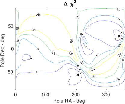
We also tested the rotation jet model (Chesley & Yeomans, 2005), which computes the non-gravitational perturbations from a discrete number of jets, whose acceleration is averaged over a nucleus rotation. For the driver of the activity we again used CO. We considered two jets, a nearly polar one at 10∘ of colatitude and a mid-latitude one on the southern hemisphere at 135∘ of colatitude. Then, we scanned a raster for the spin pole’s Right Ascension (RA) and Declination (Dec), estimating the strengths of the two jets from the fit to the astrometry.
As shown in Fig. 7, we find two minima for the pole’s RA and Dec: (, ) and (, ). Because of the larger number of parameters, the jet model provides a better fit to the data than the Marsden et al. (1973) model. However, its reliability will need to be validated by the capability of making accurate predictions. Past experience has shown that the jet model can provide more accurate comet trajectory estimates (Farnocchia et al., 2016) and therefore the jet model solutions are worth consideration, especially as the observed arc extends into late 2019 and 2020.
5 Conclusions
The pre-discovery observations of newly-discovered interstellar comet 2I/Borisov revealed a comet that is observationally quite comparable to the long-period dynamically new comets in our own solar system. We found that 2I was active at 5–7 au, indicative of the presence of accessible ices more volatile than H2O, such as CO and CO2. A subsequent comprehensive follow-up campaign, presented by Bolin et al. (2019), reinforces this conclusion. We identified a possible steep brightening at 8–9 au might indicate an onset of activity at this distance, which suggests crystallization of amorphous ice as an alternative mechanism for the activity, but more pre-discovery data, preferably from larger, multi-meter-sized telescopes, is needed to verify this behavior. We also found the nucleus to be no more than 7 km in radius, and that of the surface is currently active, both are quite typical when compared to dynamically new solar system comets occasionally discovered and observed by surveys, though the derived size of active area is highly uncertain, mainly due to the uncertainties in nucleus size and dust size distribution. The pre-discovery observations also provides stronger constraints on the inbound trajectory and non-gravitational forces of 2I. We found that a CO model provides results that are more consistent with the observations compared to H2O model.
It will be interesting to see if 2I continues to fit into the profile of dynamically new comets. For solar system comets, it is known that dynamically new comets are more likely to disintegrate than short-period comets, presumably due to their pristine state and weaker structural strength (Weissman et al., 2004). We note that independent analysis by Jewitt & Luu (2019) also suggested that 2I may be prone to disintegration based on its small nucleus size (sub-km-sized). Comets can disintegrate at large heliocentric distances, but most disintegrations seem to happen within au (Boehnhardt, 2004), a distance that 2I will reach at its perihelion in December 2019. Survived dynamically new comets also tend to fade more rapidly after perihelion (Whipple, 1978). Continued observations of 2I will enable further comparison to dynamically new comets in our solar system, and provide timely warning for any disintegration (or, as a less dramatic form, outburst) that may happen.
References
- Bar-Nun et al. (1987) Bar-Nun, A., Dror, J., Kochavi, E., & Laufer, D. 1987, Phys. Rev. B, 35, 2427, doi: 10.1103/PhysRevB.35.2427
- Bellm et al. (2019) Bellm, E. C., Kulkarni, S. R., Graham, M. J., et al. 2019, PASP, 131, 018002, doi: 10.1088/1538-3873/aaecbe
- Biver et al. (1996) Biver, N., Rauer, H., Despois, D., et al. 1996, Nature, 380, 137
- Boehnhardt (2004) Boehnhardt, H. 2004, Split comets, ed. M. C. Festou, H. U. Keller, & H. A. Weaver, 301
- Bolin et al. (2019) Bolin, B. T., Lisse, C. M., Kasliwal, M. M., et al. 2019, arXiv e-prints, arXiv:1910.14004. https://arxiv.org/abs/1910.14004
- Carpino et al. (2003) Carpino, M., Milani, A., & Chesley, S. R. 2003, Icarus, 166, 248, doi: 10.1016/S0019-1035(03)00051-4
- Chambers et al. (2016) Chambers, K. C., Magnier, E. A., Metcalfe, N., et al. 2016, arXiv e-prints, arXiv:1612.05560. https://arxiv.org/abs/1612.05560
- Chesley & Yeomans (2005) Chesley, S. R., & Yeomans, D. K. 2005, in IAU Colloq. 197: Dynamics of Populations of Planetary Systems, ed. Z. Knežević & A. Milani, 289–302
- Christensen et al. (2018) Christensen, E., Africano, B., Farneth, G., et al. 2018, in AAS/Division for Planetary Sciences Meeting Abstracts, 310.10
- Cochran et al. (2015) Cochran, A. L., Levasseur-Regourd, A.-C., Cordiner, M., et al. 2015, Space Sci. Rev., 197, 9, doi: 10.1007/s11214-015-0183-6
- Cowan & A’Hearn (1979) Cowan, J. J., & A’Hearn, M. F. 1979, Moon and Planets, 21, 155, doi: 10.1007/BF00897085
- de León et al. (2019) de León, J., Licandro, J., Serra-Ricart, M., et al. 2019, Research Notes of the American Astronomical Society, 3, 131, doi: 10.3847/2515-5172/ab449c
- Farnocchia et al. (2016) Farnocchia, D., Chesley, S. R., Micheli, M., et al. 2016, Icarus, 266, 279, doi: 10.1016/j.icarus.2015.10.035
- Fitzsimmons et al. (2018) Fitzsimmons, A., Snodgrass, C., Rozitis, B., et al. 2018, Nature Astronomy, 2, 133, doi: 10.1038/s41550-017-0361-4
- Fitzsimmons et al. (2019) Fitzsimmons, A., Hainaut, O., Meech, K., et al. 2019, arXiv e-prints, arXiv:1909.12144. https://arxiv.org/abs/1909.12144
- Fulle (2004) Fulle, M. 2004, Motion of cometary dust, ed. M. C. Festou, H. U. Keller, & H. A. Weaver, 565
- Fulle et al. (2016) Fulle, M., Altobelli, N., Buratti, B., et al. 2016, MNRAS, 462, S2, doi: 10.1093/mnras/stw1663
- Graham et al. (2019) Graham, M. J., Kulkarni, S. R., Bellm, E. C., et al. 2019, arXiv e-prints. https://arxiv.org/abs/1902.01945
- Gunnarsson et al. (2002) Gunnarsson, M., Rickman, H., Festou, M., Winnberg, A., & Tancredi, G. 2002, Icarus, 157, 309
- Guzik et al. (2019) Guzik, P., Drahus, M., Rusek, K., et al. 2019, Nature Astronomy, 467, doi: 10.1038/s41550-019-0931-8
- Jenniskens & Blake (1994) Jenniskens, P., & Blake, D. F. 1994, Science, 265, 753, doi: 10.1126/science.11539186
- Jewitt et al. (2019) Jewitt, D., Agarwal, J., Hui, M.-T., et al. 2019, AJ, 157, 65, doi: 10.3847/1538-3881/aaf38c
- Jewitt et al. (2017) Jewitt, D., Hui, M.-T., Mutchler, M., et al. 2017, ApJ, 847, L19, doi: 10.3847/2041-8213/aa88b4
- Jewitt & Luu (2019) Jewitt, D., & Luu, J. 2019, arXiv e-prints, arXiv:1910.02547. https://arxiv.org/abs/1910.02547
- Kelley et al. (2019) Kelley, M. S. P., Bodewits, D., Ye, Q., et al. 2019, in ASP Conf. Ser., Vol. 471, ADASS XXVIII, ed. P. J. Teuben, M. W. Pound, B. A. Thomas, & E. M. Warner, 305
- Krasnopolsky et al. (1987) Krasnopolsky, V. A., Moroz, V., Krysko, A., Tkachuk, A. Y., & Moreels, G. 1987, A&A, 187, 707
- Lamy et al. (2004) Lamy, P. L., Toth, I., Fernandez, Y. R., & Weaver, H. A. 2004, The sizes, shapes, albedos, and colors of cometary nuclei, ed. M. C. Festou, H. U. Keller, & H. A. Weaver, 223
- Li et al. (2013a) Li, J.-Y., A’Hearn, M. F., Belton, M. J. S., et al. 2013a, Icarus, 222, 467, doi: 10.1016/j.icarus.2012.02.011
- Li et al. (2013b) Li, J.-Y., Besse, S., A’Hearn, M. F., et al. 2013b, Icarus, 222, 559, doi: 10.1016/j.icarus.2012.11.001
- Marcus (2007) Marcus, J. N. 2007, International Comet Quarterly, 29, 39
- Marsden et al. (1973) Marsden, B. G., Sekanina, Z., & Yeomans, D. K. 1973, AJ, 78, 211, doi: 10.1086/111402
- Masci et al. (2019) Masci, F. J., Laher, R. R., Rusholme, B., et al. 2019, 131, 018003, doi: 10.1088/1538-3873/aae8ac
- McKay et al. (2019) McKay, A. J., Cochran, A. L., Dello Russo, N., & DiSanti, M. 2019, arXiv e-prints, arXiv:1910.12785. https://arxiv.org/abs/1910.12785
- Meech & Jewitt (1987) Meech, K. J., & Jewitt, D. C. 1987, A&A, 187, 585
- Meech & Svoren (2004) Meech, K. J., & Svoren, J. 2004, Using cometary activity to trace the physical and chemical evolution of cometary nuclei, ed. M. C. Festou, H. U. Keller, & H. A. Weaver, 317
- Meech et al. (2017) Meech, K. J., Weryk, R., Micheli, M., et al. 2017, Nature, 552, 378, doi: 10.1038/nature25020
- Micheli et al. (2018) Micheli, M., Farnocchia, D., Meech, K. J., et al. 2018, Nature, 559, 223, doi: 10.1038/s41586-018-0254-4
- Opitom et al. (2019) Opitom, C., Fitzsimmons, A., Jehin, E., et al. 2019, arXiv e-prints, arXiv:1910.09078. https://arxiv.org/abs/1910.09078
- ‘Oumuamua ISSI Team et al. (2019) ‘Oumuamua ISSI Team, Bannister, M. T., Bhand are, A., et al. 2019, Nature Astronomy, 3, 594, doi: 10.1038/s41550-019-0816-x
- Pätzold et al. (2016) Pätzold, M., Andert, T., Hahn, M., et al. 2016, Nature, 530, 63, doi: 10.1038/nature16535
- Prialnik & Bar-Nun (1990) Prialnik, D., & Bar-Nun, A. 1990, ApJ, 363, 274, doi: 10.1086/169339
- Seligman & Laughlin (2018) Seligman, D., & Laughlin, G. 2018, AJ, 155, 217, doi: 10.3847/1538-3881/aabd37
- Tancredi et al. (2006) Tancredi, G., Fernández, J. A., Rickman, H., & Licandro, J. 2006, Icarus, 182, 527, doi: 10.1016/j.icarus.2006.01.007
- Thomas (2009) Thomas, N. 2009, Planet. Space Sci., 57, 1106, doi: 10.1016/j.pss.2009.03.006
- Tonry et al. (2012) Tonry, J. L., Stubbs, C. W., Lykke, K. R., et al. 2012, ApJ, 750, 99, doi: 10.1088/0004-637X/750/2/99
- Weiler et al. (2003) Weiler, M., Rauer, H., Knollenberg, J., Jorda, L., & Helbert, J. 2003, A&A, 403, 313, doi: 10.1051/0004-6361:20030289
- Weissman et al. (2004) Weissman, P. R., Asphaug, E., & Lowry, S. C. 2004, Structure and density of cometary nuclei, ed. M. C. Festou, H. U. Keller, & H. A. Weaver, 337
- Whipple (1978) Whipple, F. L. 1978, Moon and Planets, 18, 343, doi: 10.1007/BF00896489
- Willmer (2018) Willmer, C. N. A. 2018, ApJS, 236, 47, doi: 10.3847/1538-4365/aabfdf
- Yabushita (1996) Yabushita, S. 1996, MNRAS, 283, 347, doi: 10.1093/mnras/283.1.347
- Ye et al. (2019) Ye, Q., Masci, F. J., Ip, W.-H., et al. 2019, arXiv e-prints, arXiv:1912.06109. https://arxiv.org/abs/1912.06109
- Ye & Hui (2014) Ye, Q.-Z., & Hui, M.-T. 2014, ApJ, 787, 115, doi: 10.1088/0004-637X/787/2/115
- Ye et al. (2017) Ye, Q.-Z., Zhang, Q., Kelley, M. S. P., & Brown, P. G. 2017, ApJ, 851, L5, doi: 10.3847/2041-8213/aa9a34
- Yeomans et al. (2004) Yeomans, D., Chodas, P., Sitarski, G., Szutowicz, S., & Królikowska, M. 2004, Comets II, 1, 137