TASTE: Temporal and Static Tensor Factorization for Phenotyping Electronic Health Records

Abstract

Phenotyping electronic health records (EHR) focuses on defining meaningful patient groups (e.g., heart failure group and diabetes group) and identifying the temporal evolution of patients in those groups. Tensor factorization has been an effective tool for phenotyping. Most of the existing works assume either a static patient representation with aggregate data or only model temporal data. However, real EHR data contain both temporal (e.g., longitudinal clinical visits) and static information (e.g., patient demographics), which are difficult to model simultaneously. In this paper, we propose Temporal And Static TEnsor factorization (TASTE) that jointly models both static and temporal information to extract phenotypes. TASTE combines the PARAFAC2 model with non-negative matrix factorization to model a temporal and a static tensor. To fit the proposed model, we transform the original problem into simpler ones which are optimally solved in an alternating fashion. For each of the sub-problems, our proposed mathematical re-formulations lead to efficient sub-problem solvers. Comprehensive experiments on large EHR data from a heart failure (HF) study confirmed that TASTE is up to $14\times$ faster than several baselines and the resulting phenotypes were confirmed to be clinically meaningful by a cardiologist. Using 80 phenotypes extracted by TASTE, a simple logistic regression can achieve the same level of area under the curve (AUC) for HF prediction compared to a deep learning model using recurrent neural networks (RNN) with 345 features.

1 Introduction

Phenotyping is about identifying patient groups sharing similar clinically-meaningful characteristics and is essential for treatment development and management [1]. However, the complexity and heterogeneity of the underlying patient information render a manual phenotyping impractical for large populations or complex conditions. Unsupervised EHR-based phenotyping based on tensor factorization, e.g.,  [2, 3, 4], provides effective alternatives. However, existing unsupervised phenotyping methods are unable to handle both static and dynamically-evolving information, which is the focus of this work.

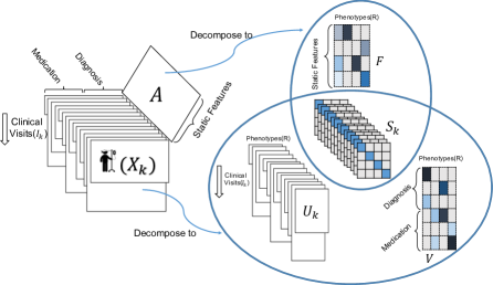
Figure 1: TASTE applied on dynamically-evolving structured EHR data and static patient information. Each $\bm{X_{k}}$ represents the medical features recorded for different clinical visits for patient k. Matrix $\bm{A}$ includes the static information (e.g., race, gender) of patients. TASTE decomposes $\{\bm{X_{k}}\}$ into three parts: $\{\bm{U_{k}}\}$, $\{\bm{S_{k}}\}$, and $\bm{V}$. Static matrix $\bm{A}$ is decomposed into two parts: $\{\bm{S_{k}}\}$ and $\bm{F}$. Note that $\{\bm{S_{k}}\}$ (personalized phenotype scores) is shared between static and dynamically-evolving features.

Traditional tensor factorization models [5, 6, 7] assume the same dimensionality along with each tensor mode. However, in practice one mode such as time can be irregular, e.g., different patients may vary by the number of clinical visits over time. To handle such longitudinal datasets, [8] and [9] propose algorithms fitting the PARAFAC2 model [10] which are faster and more scalable for handling irregular and sparse data. However, these PARAFAC2 approaches only focus on modeling the dynamically-evolving features for every patient (e.g., the structured codes recorded for every visit). Static features (such as race and gender) which do not evolve are completely neglected; yet, they are among important information in phenotyping analyses (e.g., some diseases have the higher prevalence in a certain race).

To address this problem, we propose a scalable method called TASTE which is able to jointly model both temporal and static features by combining the PARAFAC2 model with non-negative matrix factorization as shown in Figure 1. We reformulate the original non-convex problem into simpler sub-problems (i.e., orthogonal Procrustes, least square and non-negativity constrained least square) and solve each of them efficiently by avoiding unnecessary computations (e.g., expensive Khatri-Rao products).

We summarize our contributions below:

• Temporal and Static Tensor Factorization: We formulate a new technique which jointly models static and dynamic features from EHR data as nonnegative factor matrices.

• Fast and Accurate Algorithm: Our proposed fitting algorithm is up to $14\leavevmode\nobreak\ \times$ faster than the state of the art baseline. At the same time, TASTE preserves model constraints which promote model uniqueness better than baselines while maintaining interpretability.

• Case Study on Heart Failure Phenotyping: We demonstrate the practical impact of TASTE through a case study on heart failure (HF) phenotyping. We identified clinically-meaningful phenotypes confirmed by a cardiologist. Using phenotypes extracted by TASTE, simple logistic regression can achieve comparable predictive accuracy with deep learning techniques such as RNNs.

2 Background & Related Work

Table 1 summarizes the notations used in this paper.

Table 1: Notations

Symbol	Definition
*	Element-wise Multiplication
$\odot$	Khatri Rao Product
$\bm{Y},\bm{y}$	matrix, vector
$\bm{Y(i,:)}$	the $i$-th row of $\bm{Y}$
$\bm{Y(:,r)}$	the $r$-th column of $\bm{Y}$
$\bm{Y(i,r)}$	element (i,r) of $\bm{Y}$
$\bm{X_{k}}$	Feature matrix of patient $k$
$\text{diag}(\bm{Y})$	Extract the diagonal of matrix $\bm{Y}$
$\text{vec}(\bm{Y})$	Vectorizing matrix $\bm{Y}$
$\text{svd}(\bm{Y})$	Singular value decomposition on $\bm{Y}$
$||\cdot||_{F}^{2}$	Frobenius Norm
$\text{max}(0,\bm{Y})$	max operator replaces negative values in $\bm{Y}$ with 0
$\bm{Y}\geq 0$	All elements in $\bm{Y}$ are non-negative

2.1 PARAFAC2 Model

The PARAFAC2 model [11], has the following objective function:

$$\underset{\{\bm{U_{k}}\},\{\bm{S_{k}}\},\bm{V}}{\text{minimize}} \sum_{k=1}^{K}\frac{1}{2}||\bm{X_{k}}-\bm{U_{k}}\bm{S_{k}}\bm{V^{T}}||_{F}^{2}$$ (1)

subject to $$\bm{U_{k}}=\bm{Q_{k}}\bm{H},\quad\bm{Q_{k}^{T}}\bm{Q_{k}}=\bm{I},$$

where ${\small\bm{X_{k}}\in\mathbb{R}^{I_{k}\times J}}$ is the input matrix, factor matrix $\bm{U_{k}}\in\mathbb{R}^{I_{k}\times R}$, diagonal matrix $\bm{S_{k}}\in\mathbb{R}^{R\times R}$ , and factor matrix $\bm{V}\in\mathbb{R}^{J\times R}$ are output matrices. Factor matrix $\bm{Q_{k}}\in\mathbb{R}^{I_{k}\times R}$ is an orthogonal matrix, and $\bm{H}\in\mathbb{R}^{R\times R}$ where $\bm{U_{k}}=\bm{Q_{k}}\bm{H}$. SPARTan [8] is a method to fit this model for sparse datasets, as well as COPA [9] incorporates different constraints such as temporal smoothness and sparsity to the model factors to produce more meaningful results.

Uniqueness property ensures that a decomposition is pursuing the true latent factors, rather than an arbitrary rotation of them. The unconstrained version of PARAFAC2 in (1) (without constraints $\bm{U_{k}}$=$\bm{Q_{k}}$ $\bm{H}$ and $\bm{Q_{k}^{T}}$ $\bm{Q_{k}}$=$\bm{I}$ ) is not unique. Assume $\bm{B}$ as an invertible $R\times R$ matrix and $\{\bm{Z_{k}}\}$ as $R\times R$ diagonal matrices. Then, we can transform $\bm{U_{k}}\bm{S_{k}}\bm{V^{T}}$ as:

$$\bm{U_{k}}\bm{S_{k}}\bm{V^{T}}=\underbrace{(\bm{U_{k}}\bm{S_{k}}\bm{B^{-1}}\bm{Z_{k}^{-1}})}_{\bm{G_{k}}}\bm{Z_{k}}\underbrace{(\bm{B}\bm{V^{T}})}_{\bm{E^{T}}}$$

which is another valid solution achieving the same approximation error [11] - this is problematic in terms of the interpretability of the result. To promote uniqueness, Harshman [10] introduced the cross-product invariance constraint, which dictates that $\bm{U_{k}^{T}}\bm{U_{k}}$ should be constant $\forall k\in\{1,\dots,K\}$. To achieve that, the following constraint is added: $\bm{U_{k}}=\bm{Q_{k}}\bm{H}$ where $\bm{Q}_{k}^{T}\bm{Q}_{k}=\bm{I}$, so that: $\bm{U_{k}^{T}}\bm{U_{k}}=\bm{H^{T}}\bm{Q_{k}^{T}}\bm{Q_{k}}\bm{H}=\bm{H^{T}}\bm{H}=\Phi$.

2.2 Unsupervised Computational Phenotyping

A wide range of approaches applies tensor factorization techniques to extract phenotypes. [12, 2, 13, 3, 14, 15, 16] incorporate various constraints (e.g., sparsity, non-negativity, integer) into regular tensor factorization to produce more clinically-meaningful phenotypes. [8, 9] identify phenotypes and their temporal trends by using irregular tensor factorization based on PARAFAC2 [10]; yet, those approaches cannot model both dynamic and static features for meaningful phenotype extraction. As part of our experimental evaluation, we demonstrate that naively adjusting such PARAFAC2-based approaches to incorporate static information results in biased and less interpretable phenotypes. The authors of [4] proposed a collective non-negative tensor factorization for phenotyping purposes. However, the method is not able to jointly incorporate static information such as demographics with temporal features. Also they do not employ the orthogonality constraint on the temporal dimension, a strategy known to produce non-unique solutions [10, 11].

3 The TASTE framework

3.1 Intuition

We will explain the intuition of TASTE in the context of phenotyping application.

Input data include both temporal and static features for all $K$ patients:

• Temporal features ($\bm{X_{k}}$); For patient $k$, we record the medical features for different clinical visits in matrix $\bm{X_{k}}\in\mathbb{R}^{I_{k}\times J}$ where $I_{k}$ is the number of clinical visits and $J$ is the total number of medical features. Note that $I_{k}$ can be different for different patients.

• Static features ($\bm{A}$): The static features like gender, race, body mass index (BMI), smoking status are recorded in $\bm{A}\in\mathbb{R}^{K\times P}$ where $K$ is the total number of patients and $P$ is the number of static features. In particular, $\bm{A}(k,:)$ is the static features for $k^{th}$ patient.

Phenotyping process maps input data into a set of phenotypes, which involves the definition of phenotypes and temporal evolution. Figure 1 illustrates the following model interpretation. First, phenotype definitions are shared by factor matrices $\bm{V}$ and $\bm{F}$ for temporal and static features, respectively. In particular, $\bm{V(:,r)}$ or $\bm{F(:,r)}$ are the $r^{th}$ column of factor matrix $\bm{V}$ or $\bm{F}$ which indicates the participation of temporal or static features in the $r^{th}$ phenotype. Second, personalized phenotype scores for patient $k$ are provided in the diagonal matrix $\bm{S_{k}}$ where its diagonal element $\bm{S_{k}(r,r)}$ indicates the overall importance of the $r^{th}$ phenotype for patient $k$. Finally, temporal phenotype evolution for patient $k$ is specified in factor matrix $\bm{U_{k}}$ where its $r^{th}$ column $\bm{U_{k}(:,r)}$ indicates the temporal evolution of phenotype $r$ over all clinical visits of patient $k$.

3.2 Objective function and challenges

We introduce the following objective:

$$\underset{\begin{subarray}{c}\{\bm{U_{k}}\},\{\bm{Q_{k}}\},\\ \bm{H},\{\bm{S_{k}}\},\bm{V},\bm{F}\end{subarray}}{\text{minimize}} \underbrace{\sum_{k=1}^{K}\Big{(}\frac{1}{2}||\bm{X_{k}}-\bm{U_{k}}\bm{S_{k}}\bm{V^{T}}||_{F}^{2}}_{\text{PARAFAC2 (1) }}\Big{)}+\underbrace{\frac{\lambda}{2}||\bm{A}-\bm{W}\bm{F^{T}}||_{F}^{2}}_{\text{Coupled Matrix (2)}}+\underbrace{\sum_{k=1}^{K}\Big{(}\frac{\mu_{k}}{2}||\bm{U_{k}}-\bm{Q_{k}}\bm{H}||_{F}^{2}}_{\text{Uniqueness (3)}}\Big{)}$$ (2)

subject to $$\bm{Q_{k}^{T}}\bm{Q_{k}}=\bm{I},\quad\bm{U_{k}}\geq 0,\quad\bm{S_{k}}\geq 0,\quad\text{for all k=1,...,K}$$

$$\bm{W(k,:)}=\text{diag}(\bm{S_{k}})\quad\text{for all k=1,...,K}$$

$$\bm{V}\geq 0,\quad\bm{F}\geq 0$$

Objective function has three main parts as follows:

1. The first part is related to fitting a PARAFAC2 model that factorizes a set of temporal feature matrices $\bm{X_{k}}\in\mathbb{R}^{I_{k}\times J}$ into $\bm{U_{k}}\in\mathbb{R}^{I_{k}\times R}$, diagonal matrix $\bm{S_{k}}\in\mathbb{R}^{R\times R}$, and $\bm{V}\in\mathbb{R}^{J\times R}$.

2. The second part is for optimizing the static feature matrix $\bm{A}$ where ${\small\bm{A}\in\mathbb{R}^{K\times P}}$, $\bm{W}\in\mathbb{R}^{K\times R}$ and $\bm{F}\in\mathbb{R}^{P\times R}$. $\lambda$ also is the weight parameter. Common factor matrices $\{\bm{S_{k}}\}$ are shared between static and temporal features by setting $\bm{W(k,:)}$=diag($\bm{S_{k}}$).

3. The third part enforces both non-negativity of the $\bm{U_{k}}$ factor and also minimizes its difference to $\bm{Q_{k}}\bm{H}$. Due to the constraint $\bm{Q}_{k}^{T}\bm{Q}_{k}=I$, minimizing $||\bm{U}_{k}-\bm{Q}_{k}H||_{F}^{2}$ is encouraging that $\bm{U_{k}^{T}}\bm{U_{k}}$ is constant over K subjects, which is a desirable property from PARAFAC2 that promotes uniqueness, and thus enhancing interpretability [11].

4. $\lambda$ and $\mu_{k}$ are weighting parameters which all set by user. For simplicity, we set $\mu_{1}=\mu_{2}=\cdots=\mu_{K}=\mu$.

The challenge in solving the above optimization problem lies in: 1) addressing all the non-negative constraints especially on $\bm{U_{k}}$, 2) trying to make $\bm{U_{k}^{T}}$$\bm{U_{k}}$ constant over $K$ subjects by making non-negative $\bm{U_{k}}$ as close as possible to $\bm{Q_{k}}$$\bm{H}$ while $\bm{Q_{k}}$$\bm{H}$ can contain negative values, and 3) estimating all factor matrices in order to best approximate both temporal and static input matrices.

3.3 Algorithm

To optimize the objective function (2), we need to update $\{\bm{Q_{k}}\},\bm{H},\{\bm{U_{k}}\},\bm{V},$ $\{\bm{S_{k}}\},$ and $\bm{F}$ iteratively. Although the original problem in Equation 2 is non-convex, our algorithm utilizes the Block Coordinate Descent framework [17] to mathematically reformulate the objective function (2) into simpler sub-problems. In each iteration, we update $\{\bm{Q_{k}}\}$ based on Orthogonal Procrustes problem [18] which ensures an orthogonal solution for each $\bm{Q_{k}}$. Factor matrix $\bm{H}$ can be solved efficiently by least square solvers. For factor matrices $\{\bm{U_{k}}\},\bm{V},\{\bm{S_{k}}\},\bm{F}$ we reformulate objective function (2) so that the factor matrices are instances of the non-negativity constrained least squares (NNLS) problem. Each NNLS sub-problem is a convex problem and the optimal solution can be found easily. We use block principal pivoting method [19] to solve each NNLS sub-problem. The block principal pivoting method achieved state-of-the-art performance on NNLS problems compared to other optimization techniques [19]. We provide the details about NNLS problems in the supplementary material section. We also exploit structure in the underlying computations (e.g., involving Khatri-Rao products) so that each one of the sub-problems is solved efficiently. Next, we summarize the solution for each factor matrix.

3.3.1 Solution for factor matrix $\bm{Q_{k}}$

We can reformulate objective function 2 with respect to $\bm{Q_{k}}$ as follows :

$$\underset{\bm{Q_{k}}}{\text{minimize}} \mu_{k}\left\lVert\bm{U_{k}}\bm{H}^{T}-\bm{Q_{k}}\right\rVert_{F}^{2}$$ (3)

subject to $$\bm{Q_{k}^{T}}\bm{Q_{k}}=\bm{I}$$

More mathematical details about converting Equation 2 to 3 are provided in supplementary material section. The optimal value of $\bm{Q_{k}}$ can be computed via Orthogonal Procrustes problem [18] which has the closed form solution $\bm{Q_{k}}=\bm{B_{k}}\bm{C_{k}}^{T}$ where $\bm{B_{k}}\in R^{I_{k}\times R}$ and $\bm{C_{k}}\in R^{R\times R}$ are the right and left singular vectors of $\mu_{k}\bm{U_{k}}\bm{H}^{T}$. Note that each $\bm{Q_{k}}$ can contain negative values.

3.3.2 Solution for factor matrix $\bm{H}$

The objective function with respect to $\bm{H}$ can be rewritten as:

$$\underset{\bm{H}}{\text{minimize}} \sum_{k=1}^{K}\frac{\mu_{k}}{2}\left\lVert\bm{Q_{k}}^{T}\bm{U_{k}}-\bm{H}\right\rVert_{F}^{2}$$ (4)

without any constraint. The details about updating factor matrix $\bm{H}$ are provided in supplementary material section. The value of $\bm{H}$ that minimizes Equation 4 also minimizes Equation 2. The update rule for factor matrix $\bm{H}$ has the following form:

$$\bm{H}=\frac{\sum_{k=1}^{K}\mu_{k}\bm{Q_{k}}^{T}\bm{U_{k}}}{\sum_{k=1}^{K}\mu_{k}}.$$

3.3.3 Solution for phenotype evolution matrix $\bm{U_{k}}$

After updating the factor matrices $\bm{Q_{k}}$, $\bm{H}$, we focus on solving for $\bm{U_{k}}$. In classic PARAFAC2 [10, 11], this factor is retrieved through the simple multiplication $\bm{U}_{k}=\bm{Q_{k}}\bm{H}$. However, due to interpretability concern, we prefer temporal factor matrix $\bm{U}_{k}$ to be non-negative because the temporal phenotype evolution for patient k ($\bm{U_{k}}$) should never be negative. As shown in the next section, a naive enforcement of non-negativity ($max(0,\bm{Q}_{k}\leavevmode\nobreak\ \bm{H})$) violates the important uniqueness property of PARAFAC2 (the model constraints). Therefore, we consider $\bm{U_{k}}$ as an additional factor matrix, constrain it to be non-negative and minimize its difference to $\bm{Q}_{k}\bm{H}$.

The objective function with respect to $\bm{U_{k}}$ can be combined into the following NNLS form:

$$\underset{\bm{U_{k}}}{\text{minimize}} \frac{1}{2}\left\lVert\begin{bmatrix}\bm{V}\bm{S_{k}}\\ \sqrt{\mu_{k}}\bm{I}\end{bmatrix}\bm{U_{k}}^{T}-\begin{bmatrix}\bm{X_{k}}^{T}\\ \sqrt{\mu_{k}}\bm{H}^{T}\bm{Q_{k}}^{T}\end{bmatrix}\right\rVert_{F}^{2}$$ (5)

subject to $$\bm{U_{k}}\geq 0$$

As we mentioned earlier, we update factor matrix $\bm{U_{k}}$ based on block principal pivoting method.

3.3.4 Solution for temporal phenotype definition $\bm{V}$

Factor matrix $\bm{V}$ defines the participation of temporal features in different phenotypes. By considering Equation 2, factor matrix $\bm{V}$ participates in the PARAFAC2 part with non-negativity constraint. Therefore, the objective function for factor matrix $\bm{V}$ have the following form:

$$\underset{\bm{V}}{\text{minimize}} \frac{1}{2}\left\lVert\begin{bmatrix}\bm{U_{1}}\bm{S_{1}}\\ \bm{U_{2}}\bm{S_{2}}\\ .\\ \bm{U_{K}}\bm{S_{K}}\end{bmatrix}\bm{V}^{T}-\begin{bmatrix}\bm{X}_{1}\\ \bm{X}_{2}\\ .\\ \bm{X}_{K}\end{bmatrix}\right\rVert_{F}^{2}$$ (6)

subject to $$\bm{V}\geq 0$$

In order to update $\bm{V}$ based on block principal pivoting, we need to calculate $(\bm{U_{k}}\bm{S_{k}})^{T}(\bm{U_{k}}\bm{S_{k}})$ and $\bm{U_{k}}\bm{S_{k}}\bm{X_{k}}$ for all $K$ samples which can be calculated in parallel.

3.3.5 Solution for factor matrix $\bm{W}$ or $\{\bm{S}_{k}$}

The objective function with respect to $\bm{W}$ yields the following format:

$$\underset{\bm{S_{k}}}{\text{minimize}} \sum_{k=1}^{K}\Big{(}\frac{1}{2}||\bm{X_{k}}-\bm{U_{k}}\bm{S_{k}}\bm{V^{T}}||_{F}^{2}\Big{)}+\frac{\lambda}{2}||\bm{A}-\bm{W}\bm{F^{T}}||_{F}^{2}$$ (7)

subject to $$\bm{S_{k}}\geq 0$$

$$\bm{W(k,:)}=\text{diag}(\bm{S_{k}})\quad\text{for all k=1,...,K}$$

As we mentioned earlier, factor matrices $\{\bm{S_{k}}\}$ is shared between PARAFAC2 input and matrix $\bm{A}$ where $\bm{W(k,:)}$=diag($\bm{S_{k}}$). By knowing $\text{vec}(\bm{U_{k}}\bm{S_{k}}\bm{V}^{T})=(V\odot\bm{U_{k}})\bm{W(k,:)}^{T}$, Equation 7 can be rewritten as:

$$\underset{\bm{S_{k}}}{\text{minimize}} \frac{1}{2}\left\lVert\begin{bmatrix}\bm{V}\odot\bm{U_{k}}\\ \sqrt{\lambda}\bm{F}\end{bmatrix}\bm{W(k,:)}^{T}-\begin{bmatrix}\text{vec}(\bm{X_{k}})\\ \sqrt{\lambda}\bm{A(k,:)}^{T}\end{bmatrix}\right\rVert_{F}^{2}$$ (8)

subject to $$\bm{W(k,:)}\geq 0$$

where $\odot$ denotes Khatri-Rao product. We can solve the rows of factor matrix $\bm{W}$ ($\bm{W(k,:)}$ or diag($\bm{S_{k}}$)) separately and in parallel. To update each factor matrix $\bm{S_{k}}$ we need to compute two time-consuming operations: 1)$(\bm{V}\odot\bm{U_{k}})^{T}(\bm{V}\odot\bm{U_{k}})$ and 2)$(\bm{V}\odot\bm{U_{k}})^{T}\text{vec}(\bm{X_{k}})$. The first operation can be replaced with $\bm{V}^{T}\bm{V}*\bm{U_{k}}^{T}\bm{U_{k}}$ where * denotes element-wise(hadamard) product [20]. The second operation also can be replaced with $diag(\bm{U_{k}}\bm{X_{k}}\bm{V}^{T})$ [20]. Therefore, the time-consuming Khatri-Rao Product doesn’t need to be explicitly formed. Each row of W can be efficiently updated via block principal pivoting.

3.3.6 Solution for static phenotype definition $\bm{F}$

Finally, factor matrix $\bm{F}$ represents the participation of static features for the phenotypes. The objective function for factor matrix $\bm{F}$ have the following form:

$$\underset{\bm{F}}{\text{minimize}} \frac{\lambda}{2}\left\lVert\bm{W}\bm{F^{T}}-\bm{A}\right\rVert_{F}^{2}$$ (9)

subject to $$\bm{F}\geq 0$$

which can be easily updated via block principal pivoting.

3.4 Phenotype inference on new data

Given phenotype definition ($\bm{V},\bm{F}$) and factor matrix $\bm{H}$ for some training set, TASTE can project data of new unseen patients into the existing low-rank space. This is useful because healthcare provider may want to fix the phenotype definition while score new patients with those existing definitions. Moreover, such a methodology enables using the low-rank representation of patients such as ($\bm{S_{k}}$) as feature vectors for a predictive modeling task.

Suppose, $\{\bm{X_{1}},\bm{X_{2}},...,\bm{X}_{N^{{}^{\prime}}}\}$ represents the temporal information of unseen patients $\{1,2,...,N^{{}^{\prime}}\}$ and $\bm{A}^{{}^{\prime}}\in\mathbb{R}^{N^{{}^{\prime}}\times P}$ indicated their static information. TASTE is able to project the new patient’s information into the existing low-rank space ($\bm{H}$, $\bm{V}$, and $\bm{F}$) by optimizing {$\bm{Q_{n}}$}, $\{\bm{U_{n}}\}$ and $\{\bm{S_{n}}\}$ for the following objective function:

$$\underset{\begin{subarray}{c}\{\bm{Q_{n}}\},\{\bm{U_{n}}\},\\ \{\bm{S_{n}}\}\end{subarray}}{\text{minimize}} \sum_{n=1}^{N^{\prime}}\Big{(}\frac{1}{2}||\bm{X_{n}}-\bm{U_{n}}\bm{S_{n}}\bm{V^{T}}||_{F}^{2}\Big{)}+\frac{\lambda}{2}||\bm{A^{{}^{\prime}}}-\bm{W}\bm{F^{T}}||_{F}^{2}$$ (10)

$$+\sum_{n=1}^{N^{\prime}}\Big{(}\frac{\mu_{n}}{2}||\bm{U_{n}}-\bm{Q_{n}}\bm{H}||_{F}^{2}\Big{)}$$

subject to $$\bm{Q_{n}^{T}}\bm{Q_{n}}=\bm{I},\quad\text{for all }n=1,...,N^{\prime}$$

$$\bm{U_{n}}\geq 0,\quad\bm{S_{n}}\geq 0\quad\text{for all }n=1,...,N^{\prime}$$

Updating factor matrices $\{\bm{Q_{n}}\}$ is based on Equation 3. $\{\bm{U_{n}}\}$ can be minimized based on Equation 5. Finally, $\bm{W}$ can be updated based on Equation 8 where $diag(\bm{S_{n}})=W(n,:)$. Factor matrix $\bm{W}$ represents the personalized phenotype scores of all patients.

4 Experimental Results

We focus on answering the following:

1. Does TASTE preserve accuracy and the uniqueness-promoting constraint, while being fast to compute?

2. How does TASTE scale for increasing number of patients ($K$)?

3. Does the static information added in TASTE improve predictive performance for detecting heart failure?

4. Are the heart failure phenotypes produced by TASTE meaningful to an expert cardiologist?

4.1 Data Set Description

Table 2 summarizes the statistics of data sets.

Table 2: Summary statistics of two real data sets.

Dataset	# Patients	# Temporal Features	Mean($I_{k}$)	# Static Features
Sutter	59,480	1164	29	22
CMS	151,349	284	50	30

Sutter: The data set contains the EHRs for patients with new onset of heart failure and matched controls (matched by encounter time, and age). It includes 5912 cases and 59300 controls. For all patients, encounter features (e.g., medication orders, diagnosis) were extracted from the electronic health records. We use standard medical concept groupers to convert the available ICD-9 or ICD-10 codes of diagnosis to Clinical Classification Software (CCS level 3)  [21]. We also group the normalized drug names based on unique therapeutic sub-classes using the Anatomical Therapeutic Chemical (ATC) Classification System. Static information of patients includes their gender, age, race, smoking status, alcohol status and BMI.

Centers for Medicare and Medicaid (CMS): The next data set is CMS 2008-2010 Data Entrepreneurs’ Synthetic Public Use File (DE-SynPUF). The goal of CMS data set is to provide a set of realistic data by protecting the privacy of Medicare beneficiaries by using 5% of real data to synthetically construct the whole dataset. We extract the ICD-9 diagnosis codes and convert them to CCS diagnostic categories as in the case of Sutter dataset.

4.2 Evaluation metrics:

• RMSE: Accuracy is evaluated as the Root Mean Square Error (RMSE) which is a standard measure used in coupled matrix-tensor factorization literature [22, 23]. Given input collection of matrices $\bm{X_{k}}\in\mathbb{R}^{I_{k}\times J},\forall k=1,...,K$ and static input matrix $\bm{A}\in\mathbb{R}^{K\times P}$, we define

  $$\text{RMSE}=\sqrt{\frac{\sum\limits_{k=1}^{K}\sum\limits_{i=1}^{I_{k}}\sum\limits_{j=1}^{J}(\bm{X_{k}}(i,j)-\bm{\hat{X}_{k}}(i,j))^{2}+\frac{\lambda}{2}\sum\limits_{k=1}^{K}\sum\limits_{j=1}^{P}(\bm{A}(i,j)-\bm{\hat{A}}(i,j))^{2}}{\sum_{k=1}^{K}(I_{k}\times J)+K\times P}}$$ (11)

  $\bm{X_{k}}(i,j)$ denotes the $(i,j)$ element of input matrix $\bm{X_{k}}$ and $\bm{\hat{X}_{k}}(i,j)$ its approximation through a model’s factors (the $(i,j)$ element of the product $\bm{U_{k}}\bm{S_{k}}\bm{V^{T}}$ in the case of TASTE). Similarly, $\bm{A}(i,j)$ is the $(i,j)$ element of input matrix $\bm{A}$ and $\bm{\hat{A}}(i,j)$ is its approximation (in TASTE, this is the $(i,j)$ element of $\bm{W}\bm{F}^{T}$).

• Cross-Product Invariance (CPI): We use CPI to assess the solution’s uniqueness, since this is the core constraint promoting it [11]. In particular we check whether $\bm{U}_{k}^{T}\bm{U}_{k}$ is close to constant ($\bm{H^{T}}\bm{H}$) $\forall k\in\{1,\dots,K\}$). The cross-product invariance measure is defined as:

  $$\text{CPI}=1-\frac{\sum_{k=1}^{K}||\bm{U_{k}^{T}}\bm{U_{k}}-\bm{H^{T}}\bm{H}||^{2}_{F}}{\sum_{k=1}^{K}||\bm{H^{T}}\bm{H}||^{2}_{F}}.$$

  
  

  The range of cross-product invariance is between $[-\infty,1]$, with values close to 1 indicating unique solutions ($\bm{U}_{k}^{T}\bm{U}_{k}$ is close to constant).

• Area Under the ROC Curve (AUC): Examines classification model’s performance when the data is imbalance by comparing the actual and estimated labels. We use AUC on the test set to evaluate predictive model performance.

4.3 Q1. TASTE is fast, accurate and preserves uniqueness-promoting constraints

4.3.1 Baseline Approaches:

In this section, we compare TASTE with methods that incorporate non-negativity constraint on all factor matrices. Note that SPARTan [8] and COPA [9] are not able to incorporate non-negativity constraint on factor matrices $\{\bm{U_{k}}\}$.

• Cohen+ [24]: Cohen et al. proposed a PARAFAC2 framework which imposes non-negativity constraints on all factor matrices based on non-negative least squares algorithm [17]. We modified this method to handle the situation where static matrix $\bm{A}$ is coupled with PARAFAC2 input based on Figure 1. To do so, we add $\frac{\lambda}{2}||\bm{A}-\bm{W}\bm{F^{T}}||_{F}^{2}$ to their objective function and updated both factor matrices $\bm{W}$ and $\bm{F}$ in an Alternating Least Squares manner, similar to how the rest of the factors are updated in [24].

• COPA+: One simple and fast way to enforce non-negativity constraint on factor matrix $\bm{U_{k}}$ is to compute $\bm{U_{k}}$ as: $\bm{U_{k}}:=max(0,\bm{Q_{k}}\bm{H})$, where $max()$ is taken element-wise to ensure non-negative results. Therefore, we modify the implementation in [9] to handle both the PARAFAC2 input and the static matrix $\bm{A}$ and then apply the simple heuristic to make $\{\bm{U_{k}}\}$ non-negative. We will show in the experimental results section that how this heuristic method no longer guarantees unique solutions (violates model constraints).

We provide the details about tuning hyperparameters in the supplementary material section.

4.3.2 Results:

Apart from purely evaluating the RMSE and the computational time achieved, we assess to what extent the cross-product invariance constraint is satisfied  [11]. Therefore, in Figure 2 we present the average and standard deviation of RMSE, CPI, and the computational time for the approaches under comparison for Sutter and CMS data sets for four different target ranks ($R\in\{5,10,20,40\}$). In Figures  2(a), 2(b), we compare the RMSE for all three methods. We remark that all methods achieve comparable RMSE values for two different data sets. On the other hand, Figures 2(c), 2(d) show the cross-product invariance (CPI) for Sutter and CMS respectively. COPA+ achieves poor values of CPI for both data sets. This indicates that the output factors violate model constraints and would not satisfy uniqueness properties [11]. Also TASTE outperforms Cohen significantly on CPI in Figures 2(c) and 2(d). Finally, Figures 2(e), 2(f) show the running time comparison for all three methods on where TASTE is up to $4.5\times$ and $2\times$ faster than Cohen on Sutter and CMS data sets. Therefore, our approach is the only one that achieves a fast and accurate solution (in terms of RMSE) and preserves model uniqueness (in terms of CPI).

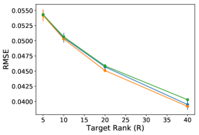
(a) RMSE for Sutter

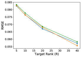
(b) RMSE for CMS

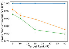
(c) CPI for Sutter

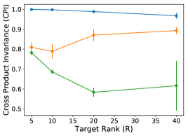
(d) CPI for CMS

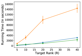
(e) Running Time for Sutter

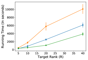
(f) Running Time for CMS

Figure 2: The average and standard deviation of RMSE (lower is better), CPI (higher is better), and total running time (in seconds) (lower is better) for different approaches and for different target ranks ($R=\{5,10,20,40\}$) related to 5 different random initialization for Sutter and CMS data sets.

4.4 Q2. TASTE is scalable

Apart from assessing the time needed for increasing values of target rank (i.e., number of phenotypes), we evaluate the approaches by comparison in terms of time needed for increasing load of input patients. Each method runs for $5$ times and the convergence threshold is set to $1e-4$ for all of them. Figure 3 compares the average and standard deviation of total running time for 125K, 250K, 500K, and 1 Million patients for $R=40$. TASTE is up to $14\times$ faster than Cohen’s baseline for $R=40$. While COPA+ is a fast approach, this baseline suffers from not satisfying model constraints which promote uniqueness.

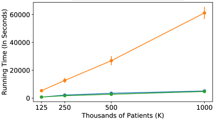
Figure 3: The average and standard deviation of running time (in seconds) for $R=40$ and for 5 random initialization by varying number of patients from 125K to 1 million for CMS data set. TASTE is upto $14\times$ faster than Cohen.

4.5 Q3. Static features in TASTE improve predictive power

We measure the performance of TASTE indirectly on the performance of classification. So we predict whether a patient will be diagnosed with heart failure (HF) or not. Our objective is to assess whether static features in the way handled by TASTE boost predictive performance by using personalized phenotype scores for all patients ($\bm{W}$) as features.

4.5.1 Cohort Construction:

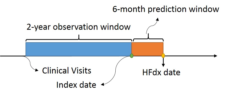
Figure 5: The arrow represents the encounter visits of a patient. We extract diagnosis and medications from a 2-year observation window by setting prediction window length to 6 months.

After applying the preprocessing steps (i.e. removing sparse features and eliminating patients with less than 5 clinical visits), we create a data set with 35113 patients where 3244 of them are cases and 31869 related to controls (9.2 % are cases). For case patients, we know the date that they are diagnosed with heart failure (HF dx). Control patients also have the same index dates as their corresponding cases. We extract 145 medications and 178 diagnosis codes from a 2-year observation window and set prediction window length to 6 months. Figure 5 in the supplementary material section depicts the observation and prediction windows in more detail.

4.5.2 Baselines:

We assess the performance of TASTE with 6 different baselines.

• RNN-regularized CNTF: CNTF [4] feeds the temporal phenotype evolution matrices ($\{\bm{U_{k}}\}$) into an LSTM model for HF prediction. This baseline only uses temporal medical features.

• RNN Baseline: We use the GRU model for HF prediction implemented in [25]. The one-hot vector format is used to represent all dynamic and static features for different clinical visits.

• Logistic regression with raw dynamic: We create a binary matrix where the rows are the number of patients and columns are the total number of medical features (323). Row $k$ of this matrix is created by aggregating over all clinical visits of matrix $\bm{X_{k}}$.

• Logistic regression with raw static+dynamic: Same as the previous approach, we create a binary matrix where the rows are number of patients and columns are the total number of temporal and static features (345) by appending matrix $\bm{A}$ to raw dynamic baseline matrix.

• COPA Personalized Score Matrix: We use the implementation of pure PARAFAC2 from [9] which learn the low-rank representation of phenotypes ($\bm{V_{copa}}$) from training set and then projecting all the new patients onto the learned phenotypic low-rank space.

• COPA (+static) Personalized Score Matrix: This is same as previous baseline, however, we incorporate the static features into PARAFAC2 matrix by repeating the value of static features of a particular patient for all encounter visits.

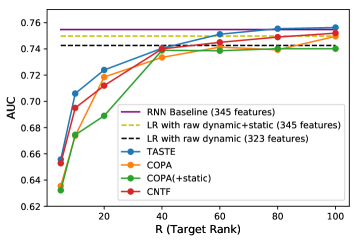
Figure 4: The average of AUC score for varying number of phenotypes (R) for TASTE and 3 other tensor baselines on the test set. The AUC score for a baseline with raw dynamic features (323) is 0.7426, for the raw dynamic+static baseline (345) is 0.7498 and for RNN baseline is 0.7547.

Results:

Figure 4 shows the average of AUC for all baselines and TASTE. For COPA, COPA(+static), CNTF and TASTE we report the AUC score for different values of R ({5,10,20,40,60,80,100}). TASTE improves the AUC score over a simple non-negative PARAFAC2 model (COPA and COPA(+static)) and CNTF which suggests: 1) incorporating static features with dynamic ones will increase the predictive power (comparison of TASTE with COPA and CNTF). 2) incorporating static features in the way we do in TASTE improves predictive power (comparison of TASTE and COPA(+static)). TASTE with R=80 (AUC=$0.7554$) performs slightly better than the RNN model. Training details are provided in the supplementary material section.

4.6 Q4. Heart Failure Phenotype Discovery

Heart failure (HF) is a complex, heterogeneous disease and is the leading cause of hospitalization in people older than 65 . However, there are no well-defined phenotypes other than the simple categorization of ejection fraction of the heart (i.e., preserved or reduced ejection fraction). With the comprehensive collection of available longitudinal EHR data, now we have the opportunity to computationally tackle the challenge of phenotyping HF patients.

4.6.1 Cohort Construction:

We select the patients diagnosed with HF from the EHRs in Sutter dataset. We extract 145 medications and 178 diagnosis codes from a 2-year observation window which ends 6 months before the heart failure diagnosis date (HFdx). The total number of patients (K) is 3,244 (the HF case patients of Sutter dataset).

4.6.2 Findings of HF Phenotypes

TASTE extracted 5 phenotypes which are all confirmed and annotated by an expert cardiologist . The clinical description of all phenotype are provided by the cardiologist:

1. Atrial Fibrillation (AF): This phenotype represents patients with irregular heartbeat and AF predisposes to HF. Medications are related to managing AF and preventing strokes. This phenotype is usually more prevalent in male and old patients (i.e. 80 years or older).

2. Hypertensive Heart Failure: This is a classic and dominant heart failure phenotype, representing a subgroup of patients with long history of hypertension, and cardiac performance declines over time. Anti-hypertensive medications are spelled out as to indicate the treatment to hypertension.

3. Obese Induced Heart Failure: This phenotype is featured by severe obesity (BMI>35) and obesity induced orthopedic condition.

4. Cardiometablic Driving Heart Failure: This phenotype is featured by diabetes and cardiometabolic conditions (i.e. hyperlipidemia, hypertension). Diabetes is a well known risk factor for cardiovascular complications (i.e. stroke, myocardial infaction, etc.), and increases the risk for heart failure.

5. Coronary Heart Disease Phenotype: This phenotype is associated with a greater deterioration of left ventricle function and a worse prognosis. This phenotype is also more prevalent in male and white population.

More detail about all phenotypes is provided in the supplementary material section.

5 Conclusions

TASTE jointly models temporal and static information from electronic health records to extract clinically meaningful phenotypes. We demonstrate the computational efficiency of our model on extensive experiments that showcase its ability to preserve important properties underpinning the model’s uniqueness, while maintaining interpretability. TASTE not only identifies clinically meaningful heart failure phenotypes validated by a cardiologist but the phenotypes also retain predictive power for predicting heart failure.

6 Acknowledgements

This work was in part supported by the National Science Foundation award IIS-1418511, CCF-1533768 and IIS-1838042, the National Institute of Health award 1R01MD011682-01 and R56HL138415.

7 Supplementary Material

7.1 Non-Negativity constrained Least Squares (NNLS)

NNLS problem has the following form:

$$\underset{\bm{C}}{\text{minimize}} \left\lVert\bm{B}\bm{C^{T}}-\bm{A}\right\rVert_{F}^{2}$$ (12)

subject to $$\bm{C}\geq 0$$

Here, $\bm{A}\in\mathbb{R}^{M\times N}$, $\bm{B}\in\mathbb{R}^{M\times R}$ and $\bm{C}\in\mathbb{R}^{N\times R}$ where $R\ll min(M,N)$. NNLS is a convex problem and the optimal solution of 12 can be easily found. In this paper, we use the block principal pivoting method [19] to solve NNLS problems. Authors showed block principal pivoting method has the state-of-the-art performance.

7.2 More details on TASTE framework

7.2.1 Updating factor matrix $\bm{Q_{k}}$

We can rewrite objective function 2 with respect to $\bm{Q_{k}}$ based on trace properties [26] as:

$$\underset{\bm{Q_{k}}}{\text{minimize}} \underbrace{\frac{\mu_{k}}{2}\text{Trace}(\bm{U_{k}}^{T}\bm{U_{k}})}_{\text{constant}}-\mu_{k}\text{Trace}(\bm{U_{k}}^{T}\bm{Q_{k}}\bm{H})$$ (13)

$$+\underbrace{\frac{\mu_{k}}{2}\text{Trace}(\bm{H}^{T}\bm{Q_{k}}^{T}\bm{Q_{k}}\bm{H})}_{\text{constant}}$$

subject to $$\bm{Q_{k}^{T}}\bm{Q_{k}}=\bm{I}$$

After removing the constant terms and applying $\text{Trace}(\bm{ABC})=\text{Trace}(\bm{CAB})$, we have:

$$\underset{\bm{Q_{k}}}{\text{minimize}} \mu_{k}\left\lVert\bm{U_{k}}\bm{H}^{T}-\bm{Q_{k}}\right\rVert_{F}^{2}$$ (14)

subject to $$\bm{Q_{k}^{T}}\bm{Q_{k}}=\bm{I}$$

7.2.2 Updating factor matrix $\bm{H}$

$\bm{Q_{k}}\in\mathbb{R}^{I_{k}\times R}$ is a rectangular orthogonal matrix ($\bm{Q_{k}}^{T}\bm{Q_{k}}=\bm{I}\in\mathbb{R}^{R\times R}$). We also introduce $\widetilde{\bm{Q_{k}}}\in\mathbb{R}^{I_{k}\times I_{k}-R}$ where $\widetilde{\bm{Q_{k}}}^{T}\widetilde{\bm{Q_{k}}}=\bm{I}\in\mathbb{R}^{I_{k}-R\times I_{k}-R}$ and $\widetilde{\bm{Q_{k}}}^{T}\bm{Q_{k}}=\bm{0}$. Now $[\bm{Q_{k}}\quad\widetilde{\bm{Q_{k}}}]$ is a square orthogonal matrix as follows:

$$\begin{bmatrix}\bm{Q_{k}}^{T}\\ \widetilde{\bm{Q_{k}}}^{T}\end{bmatrix}\begin{bmatrix}\bm{Q_{k}}\quad\widetilde{\bm{Q_{k}}}\end{bmatrix}$$ (15)

$$=\begin{bmatrix}[l]\bm{Q_{k}}^{T}\bm{Q_{k}}&\bm{Q_{k}}^{T}\widetilde{\bm{Q_{k}}}\\ \widetilde{\bm{Q_{k}}}^{T}\bm{Q_{k}}&\widetilde{\bm{Q_{k}}}^{T}\widetilde{\bm{Q_{k}}}\end{bmatrix}$$

$$=\begin{bmatrix}[l]\bm{I}_{R\times R}&0\\ 0&\bm{I}_{(I_{k}-R)\times(I_{k}-R)}\end{bmatrix}=\bm{I}_{I_{k}\times I_{k}}$$

Now we multiply $[\bm{Q_{k}}\quad\widetilde{\bm{Q_{k}}}]$ with equation LABEL:H_equation as follow:

$$\sum_{k=1}^{K}\frac{\mu_{k}}{2}\left\lVert\bm{Q_{k}}\bm{H}-\bm{U_{k}}\right\rVert_{F}^{2}$$ (16)

$$=\sum_{k=1}^{K}\frac{\mu_{k}}{2}\left\lVert[\bm{Q_{k}}\quad\widetilde{\bm{Q_{k}}}]^{T}\Big{(}\bm{Q_{k}}\bm{H}-\bm{U_{k}}\Big{)}\right\rVert_{F}^{2}$$

$$=\sum_{k=1}^{K}\frac{\mu_{k}}{2}\left\lVert\begin{bmatrix}\bm{Q_{k}}^{T}\\ \widetilde{\bm{Q_{k}}}^{T}\end{bmatrix}\Big{(}\bm{Q_{k}}\bm{H}-\bm{U_{k}}\Big{)}\right\rVert_{F}^{2}$$

$$=\sum_{k=1}^{K}\frac{\mu_{k}}{2}\left\lVert\begin{bmatrix}\bm{Q_{k}}^{T}\bm{Q_{k}}\\ \widetilde{\bm{Q_{k}}}^{T}\bm{Q_{k}}\end{bmatrix}\bm{H}-\begin{bmatrix}\bm{Q_{k}}^{T}\bm{U_{k}}\\ \widetilde{\bm{Q_{k}}}^{T}\bm{U_{k}}\end{bmatrix}\right\rVert_{F}^{2}$$

$$=\sum_{k=1}^{K}\Big{(}\frac{\mu_{k}}{2}\left\lVert\bm{H}-\bm{Q_{k}}^{T}\bm{U_{k}}\right\rVert_{F}^{2}+\overbrace{\left\lVert\widetilde{\bm{Q_{k}}}^{T}\bm{U_{k}}\right\rVert_{F}^{2}}^{\text{constant}}\Big{)}$$

where $\sum_{k=1}^{K}\left\lVert\widetilde{\bm{Q_{k}}}^{T}\bm{U_{k}}\right\rVert_{F}^{2}$ is a constant and independent of the parameter under minimization. Therefore, the value of $\bm{H}$ that minimizes $\sum_{k=1}^{K}\frac{\mu_{k}}{2}\left\lVert\bm{Q_{k}}\bm{H}-\bm{U_{k}}\right\rVert_{F}^{2}$ also minimizes $\sum_{k=1}^{K}\frac{\mu_{k}}{2}\left\lVert\bm{H}-\bm{Q_{k}}^{T}\bm{U_{k}}\right\rVert_{F}^{2}$

7.3 Implementation details

TASTE is implemented in MATLAB. To enable reproducibility of our work, we attached a zip file containing TASTE code. All the approaches (including the baselines) are evaluated on MatlabR2017b. We utilize the capabilities of Parallel Computing Toolbox of Matlab by activating parallel pool for all methods. For Sutter and CMS dataset, we used 12 workers. For the prediction task, we use the implementation of regularized logistic regression from Scikit-learn machine learning library of python 3.6.

Table 3: TASTE extracted 5 phenotypes from the HF dataset. Red indicates the static features; $Dx\_$ indicates diagnoses; $Rx\_$ indicates medication; The phenotype names are provided by the cardiologist.

P1. Atrial Fibrillation (AF)	Weight
Dx_Cardiac dysrhythmias [106.]	1
Rx_Coumarin Anticoagulants	0.79597
Dx_Heart valve disorders [96.]	0.57526
Dx_Coronary atherosclerosis and other heart disease [101.]	0.465406
Rx_Beta Blockers Cardio-Selective	0.348005
Dx_Conduction disorders [105.]	0.246467
Static_white	0.270443
Static_age_greater_80	0.245424
Static_Non_Hispanic	0.245373
Static_male	0.200464
Static_Alchohol_yes	0.197431
Static_Smk_Quit	0.167838
P2. Hypertensive Heart Failure:	Weight
Dx_Essential hypertension [98.]	0.705933
Rx_Calcium Channel Blockers	0.684211
Rx_ACE Inhibitors	0.578426
Rx_Beta Blockers Cardio-Selective	0.564413
Rx_Angiotensin II Receptor Antagonists	0.250883
Dx_Chronic kidney disease [158.]	0.14528
Rx_Thiazides and Thiazide-Like Diuretics	0.134521
Static_Non_Hispanic	0.536399
Static_female	0.390343
Static_Smk_NO	0.363068
Static_Alchohol_No	0.360158
Static_white	0.345942
Static_Alchohol_yes	0.264664
Static_age_between_70_79	0.26237
Static_Severely_obese	0.252981
P3. Obese Induced Heart Failure:	Weight
Dx_Other back problems	0.438879
Rx_Opioid Combinations	0.414518
Dx_Other connective tissue disease [211.]	0.304155
Dx_Other non-traumatic joint disorders [204.]	0.269159
Dx_Osteoarthritis [203.]	0.190075
Rx_Opioid Agonists	0.185262
Dx_Intervertebral disc disorders	0.156421
Rx_Benzodiazepines	0.150865
Static_female	0.548758
Static_Non_Hispanic	0.52183
Static_white	0.474545
Static_Alchohol_No	0.404191
Static_Smk_Quit	0.273576
Static_Severely_obese	0.226485
Static_age_between_70_79	0.180683
Static_age_between_60_69	0.180006
P4. Cardiometablic Driving Heart Failure:	Weight
Dx_Diabetes mellitus without complication [49.]	0.712628
Dx_Disorders of lipid metabolism [53.]	0.507946
Rx_Biguanides	0.48821
Dx_Immunizations and screening for infectious disease [10.]	0.358349
Rx_Diagnostic Tests	0.353441
Static_Alchohol_No	0.247165
Static_Non_Hispanic	0.190547
Static_Smk_NO	0.184782
Static_male	0.164795
Static_white	0.15693
Static_age_between_60_69	0.131118
P5. Coronary Heart Disease Phenotype:	Weight
Dx_Disorders of lipid metabolism [53.]	0.984987
Rx_HMG CoA Reductase Inhibitors	0.442637
Dx_Coronary atherosclerosis and other heart disease [101.]	0.265414
Dx_Diabetes with renal manifestations	0.229549
Dx_Chronic kidney disease [158.]	0.203386
Dx_Other thyroid disorders	0.101615
Static_Non_Hispanic	1
Static_white	0.998604
Static_male	0.957132
Static_Smk_Quit	0.773904
Static_Alchohol_yes	0.604641

7.4 More details on Q1. TASTE is fast, accurate and preserves uniqueness-promoting constraints

7.4.1 Setting hyper-parameters:

We perform a grid search for $\lambda\in\{0.01,0.1,1\}$ and $\mu_{1}=\dots=\mu_{K}=\mu\in\{0.01,0.1,1\}$ for TASTE and Cohen+ for different target ranks ($R=\{5,10,20,40\}$) and we run each method with specific parameter for 5 random initialization and pick the best values of $\lambda$ and $\mu$ based on the lowest average RMSE value. For COPA+, we just search for the best value of $\lambda\in\{0.1,1,10\}$ since it does not require $\mu$ parameter.

7.5 More details on Q3. Static features in TASTE improve predictive power

7.5.1 Training Details:

We train a Lasso Logistic Regression for all the baselines under comparison. We divide the patient records into training ($75\%$), validation ($10\%$), and test sets ($15\%$) and use them to evaluate all baselines. Lasso Logistic Regression has regularization parameter ($C=[1e-2,1e-1,1,10,100,1000,10000]$). For all 6 baselines, we just need to tune parameter $C$. However, for TASTE we need to perform a 3-D grid search over $\lambda\in\{0.01,0.1,1\}$ and $\mu_{1}=\mu_{2}=\dots=\mu_{K}=\mu=\in\{0.01,0.1,1\}$ and $C$. We first train TASTE on training set and learn the phenotype low-rank representation ($\bm{V}$, $\bm{F}$) and then train Lasso Logistic Regression classifier based on patient low-rank representation ($\bm{W_{train}}$) and corresponding labels. Then we project the patients in validation set on phenotype low-rank representation and learn their personalized phenotype scores $\bm{W_{val}}$. Next, we feed $\bm{W_{val}}$ into a Lasso Logistic Regression and calculate the AUC score. Finally, we pick the best parameters based on the highest AUC score on validation set and report the AUC on test data. The training phase for COPA, COPA(+static) and CNTF is same as TASTE.

7.6 More details on Q4. Heart Failure Phenotype Discovery

7.6.1 Hyper-parameter search:

The optimal number of phenotypes (R), $\lambda$, and $\mu$ need to be tuned. So, We perform a 3-D grid search for $R=\{3,4,5,...,20\}$, $\lambda\in\{0.01,0.1,1\}$ and $\mu_{1}=\mu_{2}=\cdots=\mu_{K}=\mu=\in\{0.01,0.1,1\}$ based on the stability-driven metric provided in [27]. Stability-driven metric calculates the dissimilarity between a pair of factor matrices from two different initialization ($\bm{V}$,$\bm{V}$’) using the cross-correlation matrix (C) as follows: $diss(\bm{V},\bm{V}^{\prime})=\frac{1}{2R}\Big{(}2R-\sum_{i=1}^{R}\underset{1\leq j\leq R}{\max}C_{ij}-\sum_{j=1}^{R}\underset{1\leq i\leq R}{\max}C_{ij}\Big{)}$ where diss($\bm{V}$,$\bm{V}$’) denotes the dissimilarity between factor matrices $\bm{V}$,$\bm{V}$’. Also cross-correlation matrix ($\bm{C}\in\mathbb{R}^{R\times R}$) computes the cosine similarity between all columns of $\bm{V}$,$\bm{V}$’. We run TASTE model for 10 different random initialization and compute the average dissimilarity for each value of $R$, $\lambda$, and $\mu$. Figure 6 shows the best value of stability-driven metric for different values for R. The best solution corresponding to $R=5,\lambda=0.1,\mu=0.1$ were chosen as the one achieving the lowest average dissimilarity. Then, for fixed $R=5,\lambda=0.1,\mu=0.1$ we present the phenotypes of the model achieving the lowest RMSE among the 10 different runs.

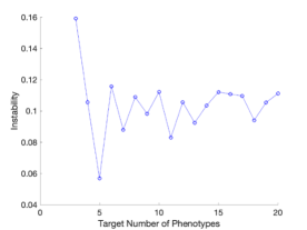
Figure 6: Stability-driven metric for different values of phenotypes($R=\{3,4,...,20\}$). The optimal value of phenotypes corresponds to the minimum value of stability-driven metric ($R=5$).

7.6.2 Phenotype definition:

We provide the details of all 5 phenotypes discovered by TASTE in Table 3.

7.6.3 Pure PARAFAC2 cannot handle static feature integration.

In this Section, we illustrate the fact that a naive way of incorporating static feature information into a simpler PARAFAC2-based framework [9] would result in poor, less interpretable phenotypes. We incorporate the static features into PARAFAC2 input by repeating the value of static features on all clinical visits of the patients same as what we did for COPA(+static). For instance, if the male feature of patient k has value 1, we repeat the value 1 for all the clinical visits of that patient. Then we compare the phenotype definitions discovered by TASTE (matrices $\bm{V}$, $\bm{F}$) and by COPA (matrix $\bm{V}$). Table 4 contains two sample phenotypes discovered by this baseline, using the same truncation threshold that we use throughout this work (we only consider features with values greater than $0.1$). We observe that the static features introduce a significant amount of bias into the resulting phenotypes: the phenotype definitions are essentially dominated by static features, while the values of weights corresponding to dynamic features are closer to $0$. This suggests that pure PARAFAC2-based models such as the work in [9] are unable to produce meaningful phenotypes that handle both static and dynamic features. Such a conclusion extends to other PARAFAC2-based work which does not explicitly model side information [11, 8, 24].

Table 4: Two sample phenotypes discovered by COPA(+static) baseline by naively integrating static features into a simpler PARAFAC2-based model [9] .

Phenotype 1	weight
Static_Alcohol_yes	0.3860
Static_White	0.2160
Static_Non_Hispanic	0.2064
Static_Smk_Quit	0.1743
Static_male	0.1508
Static_moderately_obese	0.1025
Phenotype 2	weight
Static_age_between_70_79	1
Static_Non_Hispanic	0.8233
Static_White	0.7502
Static_Alcohol_No	0.6905
Static_moderately_obese	0.2098
Static_male	0.2026
Static_Smk_No	0.1614

7.7 Recovery of true factor matrices

In this section, we assess to what extent the original factor matrices can be recovered through synthetic data experiments . We demonstrate that: a) TASTE recovers the true latent factors more accurately than baselines for noisy data; and b) the baseline (COPA+) which does not preserve a high CPI measure (which is known to be theoretically linked to uniqueness [11] ) fails to match TASTE in terms of latent factor recovery, despite achieving similar RMSE.

7.7.1 Evaluation Metric:

Similarity between two factor matrices: We define the cosine similarity between two vectors $\bm{x_{i}}$, $\bm{y_{j}}$ as $C_{ij}$ =$\frac{\bm{x_{i}}^{T}\bm{y_{j}}}{||x_{i}||||y_{j}||}$. Then the similarity between two factor matrices $\bm{X}\in\mathbb{R}^{I\times R}$, $\bm{Y}\in\mathbb{R}^{I\times R}$ can be computed as (similar to [11]):

$$\text{Sim}(\bm{X},\bm{Y})=\frac{\sum\limits_{i=1}^{R}\underset{1\leq j\leq R}{\max}C_{ij}}{R}$$

The range of $Sim$ is between [0,1] and the values near 1 indicate higher similarity.

7.7.2 Synthetic Data Construction:

We construct the ground-truth factor matrices $\bm{\tilde{H}}\in\mathbb{R}^{R\times R}$, $\bm{\tilde{V}}\in\mathbb{R}^{J\times R}$, $\bm{\tilde{W}}\in\mathbb{R}^{K\times R}$, $\bm{\tilde{F}}\in\mathbb{R}^{P\times R}$ by drawing a number uniformly at random between (0,1) to each element of each matrix. For each factor matrix $\bm{\tilde{Q}_{k}}$, we create a binary non-negative matrix such that $\bm{\tilde{Q}_{k}}^{T}\bm{\tilde{Q}_{k}}=I$ and then compute $\bm{\tilde{U}_{k}}$=$\bm{\tilde{Q}_{k}}$$\bm{\tilde{H}}$. After constructing all factor matrices, we compute the input based on $\bm{X_{k}=\bm{\tilde{U}_{k}}diag(\tilde{W}(k,:))\bm{\tilde{V}}^{T}}$ and $\bm{A}=\bm{\tilde{W}}\bm{\tilde{F}}^{T}$. We set $K=100,J=30,P=20,I_{k}=100$, and $R=4$. We then add Gaussian normal noise to varying percentages of randomly-drawn elements ($\{5\%,10\%,15\%,20\%,25\%,30\%,35\%,40\%\}$) of $\bm{X}_{k},\forall k=1,\dots,K$ and $\bm{A}$ input matrices.

7.7.3 Results:

For all approaches under comparison, all three methods achieve same value for RMSE, therefore, we skip ploting RMSE vs different noise levels. We assess the similarity measure between each ground truth latent factor and its corresponding estimated one (e.g., $Sim(\bm{\tilde{V}},\bm{V})$), and consider the average $Sim(\cdot,\cdot)$ measure across all output factors as shown in Figure 7(a). We also measure CPI and provide the results in 7(b) for different levels of noise . We observe that despite achieving comparable RMSE, COPA+ scores the lowest on the similarity between the true and the estimated factors. On the other hand, TASTE achieves the highest amount of recovery, in accordance to the fact that it achieves the highest CPI among all approaches. Overall, we demonstrate how promoting uniqueness (by enforcing the CPI measure to be preserved [11]) leads to more accurate parameter recovery, as suggested by prior work [11, 28].

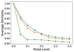
(a) Average Similarity vs Noise Level

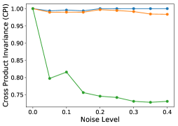
(b) CPI vs Noise Level

Figure 7: Figure 7(a) provides total average similarity between the estimated and the true factor matrices for different noise levels ($\{5\%,10\%,15\%,20\%,25\%,30\%,35\%,40\%\}$) on synthetic data. Figure 7(b) provides the CPI of three methods for different levels of noise for a synthetic data with K=100, J=30, P=20, $I_{k}=100$, R=4. All points in the figures is computed as an average of 5 random initialization. All three algorithms achieve similar values for RMSE.

References

- [1] Rachel L Richesson, Jimeng Sun, Jyotishman Pathak, Abel N Kho, and Joshua C Denny. Clinical phenotyping in selected national networks: demonstrating the need for high-throughput, portable, and computational methods. Artificial intelligence in medicine, 71:57–61, 2016.
- [2] Joyce C Ho, Joydeep Ghosh, and Jimeng Sun. Marble: high-throughput phenotyping from electronic health records via sparse nonnegative tensor factorization. In KDD, pages 115–124. ACM, 2014.
- [3] Ioakeim Perros, Evangelos E. Papalexakis, Haesun Park, Richard Vuduc, Xiaowei Yan, Christopher Defilippi, Walter F. Stewart, and Jimeng Sun. Sustain: Scalable unsupervised scoring for tensors and its application to phenotyping. In Proceedings of the 24th ACM SIGKDD International Conference on Knowledge Discovery & Data Mining, KDD ’18, pages 2080–2089, New York, NY, USA, 2018. ACM.
- [4] K. Yin, D. Qian, W. K. Cheung, B. C. M. Fung, and J. Poon. Learning phenotypes and dynamic patient representations via rnn regularized collective non-negative tensor factorization. In AAAI, Honolulu, HI, January 2019.
- [5] J Douglas Carroll and Jih-Jie Chang. Analysis of individual differences in multidimensional scaling via an n-way generalization of “eckart-young” decomposition. Psychometrika, 35(3):283–319, 1970.
- [6] Frank L Hitchcock. The expression of a tensor or a polyadic as a sum of products. Journal of Mathematics and Physics, 6(1-4):164–189, 1927.
- [7] Richard A Harshman. Foundations of the parafac procedure: Models and conditions for an" explanatory" multimodal factor analysis. 1970.
- [8] Ioakeim Perros, Evangelos E Papalexakis, Fei Wang, Richard Vuduc, Elizabeth Searles, Michael Thompson, and Jimeng Sun. SPARTan: Scalable PARAFAC2 for large & sparse data. In KDD, KDD ’17, pages 375–384. ACM, 2017.
- [9] Ardavan Afshar, Ioakeim Perros, Evangelos E. Papalexakis, Elizabeth Searles, Joyce Ho, and Jimeng Sun. COPA: Constrained parafac2 for sparse & large datasets. CIKM ’18, pages 793–802, New York, NY, USA, 2018. ACM.
- [10] R. A. Harshman. PARAFAC2: Mathematical and technical notes. UCLA Working Papers in Phonetics, 22:30–44, 1972.
- [11] Henk AL Kiers, Jos MF Ten Berge, and Rasmus Bro. Parafac2-part i. a direct fitting algorithm for the parafac2 model. Journal of Chemometrics, 13(3-4):275–294, 1999.
- [12] Joyce C Ho, Joydeep Ghosh, Steve R Steinhubl, Walter F Stewart, Joshua C Denny, Bradley A Malin, and Jimeng Sun. Limestone: High-throughput candidate phenotype generation via tensor factorization. Journal of biomedical informatics, 52:199–211, 2014.
- [13] Jette Henderson, Joyce C Ho, Abel N Kho, Joshua C Denny, Bradley A Malin, Jimeng Sun, and Joydeep Ghosh. Granite: Diversified, sparse tensor factorization for electronic health record-based phenotyping. In (ICHI), 2017, pages 214–223. IEEE, 2017.
- [14] Juan Zhao, Yun Zhang, David J Schlueter, Patrick Wu, Vern Eric Kerchberger, S Trent Rosenbloom, Quinn S Wells, QiPing Feng, Joshua C Denny, and Wei-Qi Wei. Detecting time-evolving phenotypic topics via tensor factorization on electronic health records: Cardiovascular disease case study. Journal of biomedical informatics, 98:103270, 2019.
- [15] Juan Zhao, QiPing Feng, Patrick Wu, Jeremy L Warner, Joshua C Denny, and Wei-Qi Wei. Using topic modeling via non-negative matrix factorization to identify relationships between genetic variants and disease phenotypes: A case study of lipoprotein (a)(lpa). PloS one, 14(2):e0212112, 2019.
- [16] Xiaoqian Jiang, Samden Lhatoo, Guo-Qiang Zhang, Luyao Chen, and Yejin Kim. Combining representation learning with tensor factorization for risk factor analysis-an application to epilepsy and alzheimer’s disease. arXiv preprint arXiv:1905.05830, 2019.
- [17] Jingu Kim, Yunlong He, and Haesun Park. Algorithms for nonnegative matrix and tensor factorizations: A unified view based on block coordinate descent framework. Journal of Global Optimization, 58(2):285–319, 2014.
- [18] Peter H Schönemann. A generalized solution of the orthogonal procrustes problem. Psychometrika, 31(1):1–10, 1966.
- [19] Jingu Kim and Haesun Park. Fast nonnegative matrix factorization: An active-set-like method and comparisons. SIAM Journal on Scientific Computing, 33(6):3261–3281, 2011.
- [20] Charles F Van Loan. The ubiquitous kronecker product. Journal of computational and applied mathematics, 123(1-2):85–100, 2000.
- [21] Vergil N Slee. The international classification of diseases: ninth revision (icd-9). Annals of internal medicine, 88(3):424–426, 1978.
- [22] Dongjin Choi, Jun-Gi Jang, and U Kang. Fast, accurate, and scalable method for sparse coupled matrix-tensor factorization. arXiv preprint arXiv:1708.08640, 2017.
- [23] Alex Beutel, Partha Pratim Talukdar, Abhimanu Kumar, Christos Faloutsos, Evangelos E Papalexakis, and Eric P Xing. Flexifact: Scalable flexible factorization of coupled tensors on hadoop. In Proceedings of the 2014 SIAM International Conference on Data Mining, pages 109–117. SIAM, 2014.
- [24] Jeremy E Cohen and Rasmus Bro. Nonnegative parafac2: a flexible coupling approach. In International Conference on Latent Variable Analysis and Signal Separation, pages 89–98. Springer, 2018.
- [25] Edward Choi, Andy Schuetz, Walter F Stewart, and Jimeng Sun. Using recurrent neural network models for early detection of heart failure onset. Journal of the American Medical Informatics Association, 24(2):361–370, 2016.
- [26] Kaare Brandt Petersen, Michael Syskind Pedersen, et al. The matrix cookbook. Technical University of Denmark, 7(15):510, 2008.
- [27] Siqi Wu, Antony Joseph, Ann S Hammonds, Susan E Celniker, Bin Yu, and Erwin Frise. Stability-driven nonnegative matrix factorization to interpret spatial gene expression and build local gene networks. Proceedings of the National Academy of Sciences, 113(16):4290–4295, 2016.
- [28] Alex H Williams, Tony Hyun Kim, Forea Wang, Saurabh Vyas, Stephen I Ryu, Krishna V Shenoy, Mark Schnitzer, Tamara G Kolda, and Surya Ganguli. Unsupervised discovery of demixed, low-dimensional neural dynamics across multiple timescales through tensor component analysis. Neuron, 2018.