∎
22email: beattie@vt.edu 33institutetext: Z. Drmač 44institutetext: Faculty of Science, Department of Mathematics, University of Zagreb, Zagreb, 10000, Croatia
44email: drmac@math.hr 55institutetext: S. Gugercin 66institutetext: Department of Mathematics and Division of Computational Modeling and Data Analytics, Virginia Tech, Blacksburg, VA, 24061, USA
66email: gugercin@vt.edu
Revisiting IRKA:
Connections with pole placement and backward stability††thanks: The work of Beattie was supported in parts by NSF through Grant DMS-1819110.
The work of Drmač was supported in parts by the the DARPA Contract HR0011-16-C-0116 “On a Data-Driven, Operator-Theoretic Framework for Space-Time Analysis of Process Dynamics” and the DARPA Contract HR0011-18-9-0033 “The Physics of Artificial Intelligence”.
The work of Gugercin was supported in parts by NSF through Grant DMS-1720257 and DMS-1819110.
Abstract
The iterative rational Krylov algorithm (IRKA) is a popular approach for producing locally optimal reduced-order -approximations to linear time-invariant (LTI) dynamical systems. Overall, IRKA has seen significant practical success in computing high fidelity (locally) optimal reduced models and has been successfully applied in a variety of large-scale settings. Moreover, IRKA has provided a foundation for recent extensions to the systematic model reduction of bilinear and nonlinear dynamical systems.
Convergence of the basic IRKA iteration is generally observed to be rapid — but not always; and despite the simplicity of the iteration, its convergence behavior is remarkably complex and not well understood aside from a few special cases. The overall effectiveness and computational robustness of the basic IRKA iteration is surprising since its algorithmic goals are very similar to a pole assignment problem, which can be notoriously ill-conditioned. We investigate this connection here and discuss a variety of nice properties of the IRKA iteration that are revealed when the iteration is framed with respect to a primitive basis. We find that the connection with pole assignment suggests refinements to the basic algorithm that can improve convergence behavior, leading also to new choices for termination criteria that assure backward stability.
Keywords:
Interpolation Model Reduction -optimality Pole placement Backward stability1 Introduction
The iterative rational Krylov algorithm (IRKA) was introduced in Gugercin_Antoulas_Beattie:2008:IRKA as an approach for producing locally optimal reduced-order -approximations to linear time-invariant (LTI) dynamical systems given, say, as
| (1) |
where , and . We will assume that the dynamical system is stable, i.e., all the eigenvalues of have negative real parts. The cases of interest will be when is very large, and we seek a substantially lower order dynamical system, say,
| (2) |
with , and . One seeks a realization (2) so that the reduced system order and the reduced system output uniformly well over all inputs with .
Projection-based model reduction is a common framework to obtain reduced models: Given the full model (1), construct two model reduction bases with invertible. Then the reduced model quantities in (2) are given by
| (3) |
The following question arises: How to choose and so that the reduced model is a high-fidelity approximation to the original one? There are many different ways to construct and , and we refer the reader to antoulas2005approximation ; AntBG20 ; MORBook for detailed descriptions of such methods for linear dynamical systems. Here we focus on constructing optimal interpolatory reduced models.
To discuss interpolation and optimality, we first need to define the concept of transfer function. Let , , and denote the Laplace transforms of , , and , respectively. Taking the Laplace transforms of (1) and (2) yields
| (4) | ||||
| (5) |
The rational functions and are the transfer functions associated with the full model (1) and the reduced model (2). While is a degree- rational function, is of degree-.
Interpolatory model reduction aims to construct an that interpolates at selected points in the complex plane. Indeed, we will focus on Hermite interpolation, as this will be tied to optimality later. Suppose we are given mutually distinct interpolation points (also called shifts), , in the complex plane. We will assume that the shifts have positive real parts and that are closed (as a set) under conjugation, i.e., there exists an index permutation such that .
Given , construct the model reduction bases and such that
| (6) | ||||
| (7) |
Then, the reduced model (2) constructed as in (3) satisfies
| (8) |
In other words, is a rational Hermite interpolant to at the specified interpolation points. However, this construction requires knowing the interpolation points. How should one choose them to guarantee a high-fidelity reduced model?
We will measure fidelity using the norm: The norm of a dynamical system with transfer function is defined as
For the full model (1) and the reduced model (2), the output error satisfies
where and . So, a reduced model that minimizes the distance is guaranteed to yield uniformly good approximations over finite energy inputs. Therefore, it is desirable to find a reduced model with transfer function that minimizes the distance, i.e., to find such that
at least locally in a neighborhood of . This is a heavily studied topic; see, e.g., wilson1970optimum ; hyland1985theoptimal ; zigic1993contragredient ; spanos1992anewalgorithm ; benner_sylvester for Sylvester-equation formulation and meieriii1967approximation ; Gugercin_Antoulas_Beattie:2008:IRKA ; vandooren2008hom ; bunse-gerstner2009hom ; beattie2012realization ; krajewski1995program ; xu2010optimal for interpolation formulation. Indeed, these two formulations are equivalent as shown in Gugercin_Antoulas_Beattie:2008:IRKA and we focus on the interpolatory formulation.
How does the optimality relate to Hermite interpolation? Let be the eigenvalues of , assumed simple. If is an -optimal approximation to , then it is a Hermite interpolant to at the points , i.e.,
| (9) |
These conditions are known as Meier-Luenberger conditions for optimality meieriii1967approximation . However, one cannot simply use in constructing and in (6)-(7) since s are not known a priori. This requires an iteratively corrected algorithm. The iterative rational Krylov algorithm IRKA Gugercin_Antoulas_Beattie:2008:IRKA as outlined in Algorithm 1 precisely achieves this task. It reflects the intermediate interpolation points until the required optimality criterion, i.e., is met. Upon convergence, the reduced model is a locally optimal -approximation to (2). IRKA has been successful in producing locally optimal reduced models at a modest cost and many variants have been proposed; see, e.g., beattie2007kbm ; beattie2009trm ; beattie2012realization ; panzer2013 ; HokMag2018 ; poussot2011iterative ; vuillemin2013h2 ; breiten2013near ; gugercin2008isk ; goyal2019time . Moreover, it has been successfully extended to model reduction of bilinear breiten12 ; flagg15 and quadratic-bilinear systems benner2018h2 , two important classes of structured nonlinear systems.
Our goal in this paper is not to compare model reduction techniques, nor is it to illustrate effectiveness of IRKA and its variants. Refer to sources cited above for such analyses. Our main goal here is to revisit IRKA in its original form and reveal new connections to the pole placement problem (Section 3) by a thorough analysis of the quantities involved in a special basis (Section 2). This will lead to a backward stability formulation relating then to new stopping criteria (Section 4).
2 Structure in the primitive bases
In Steps 3 and 4 of IRKA as laid out in Algorithm 1 above, the matrices and are each chosen as bases for a pair of rational Krylov subspaces. The reduced model is independent of the particular bases chosen and one usually constructs them to be orthonormal. We consider a different choice in this section, and show that if and are chosen instead as primitive bases, i.e., if
| (10) |
then the state-space realization of the reduced model exhibits an important structure which forms the foundation of our analysis that follows in Sections 3 and 4. Therefore, in the rest of the paper, we use primitive bases for and as given in (10). We emphasize that this does not change the reduced model ; it is simply a change of basis that reveals nontrivial structure that can be exploited both in the theoretical analysis of the algorithm and for its efficient software implementation.
It is easy to check that (Gugercin_Antoulas_Beattie:2008:IRKA ), for and as primitive bases (10), the matrices and are symmetric; but not necessarily Hermitian. Moreover, one may directly verify that (abg10 ), is the Loewner matrix whose th entry, for , is given by
| (11) |
with the convention that .
Lemma 1
Let be the nodal polynomial associated with the shifts . For any monic polynomial , define the vector
and the matrix with . Then and
| (12) | |||||
| (13) |
Proof
Pick any index and consider . Evidently, and so the Lagrange interpolant on is exact:
Divide by and rearrange to obtain
| (14) |
Let be a Jordan curve that separates into two open, simply-connected sets, with containing all the eigenvalues of and containing both the point at and the shifts . For any function that is analytic in a compact set containing , can be defined as Applying this to (14) gives
Postmultiplication by provides the column of (12), while premultiplication by (and since commutes with ) provides the row of (13).
To compute the characteristic polynomial of , we use the alternative factorizations111For the reader’s convenience, here we actually reproduce the proof of the Sherman–Morrison determinant formula.,
where . Then we have that
where the last equality follows by observing that the penultimate expression describes a monic polynomial of degree that interpolates at .
Lemma 1, and more specifically (12) and (13), reveal the rational Krylov structure arising from the choice of and in (10). At first, connection of the involved quantities such as the vector to IRKA quantities might not be clear. In the following result, we make these connections precise.
Lemma 2
Let the reduced model be obtained by projection as in (3) using the primitive bases and in (10). Let
Then (12) and (13) hold with . In particular, and . Moreover, if is an eigenvalue of , then
| (16) |
is an associated (right) eigenvector of for . Similarly, the vector
| (17) |
is an associated left eigenvector of , for , with , and is the residue of at , i.e., .
Proof
Now, choose a monic polynomial so that . Then (12) and (13) hold with an associated as given in Lemma 1. But then applying to (12) yields . This in turn implies .
Suppose that is an eigenvalue of . Directly substitute and use (2) with to obtain
Thus, is a right eigenvector for associated with . Note that also solves the generalized eigenvalue problems:
| (18) |
(18a) is immediate from the definition of . (18b) is obtained by transposition of (18a) and using the facts that and are symmetric. Notice that (18b) shows that is a left eigenvector for associated with . On the other hand, direct substitution also shows that
so is also a left eigenvector of associated with . We must have then
for some scalar which we now determine. Using (11) and (16), the component of each side of the equation can be expressed as
| (19) |
Define the function . It is easily checked that is a polynomial of degree and so Lagrange interpolation on is exact:
Now evaluate this expression at :
where we observe that . Comparing this expression to (19) we find .
Lemma 2 illustrates that if the primitive bases and in (10) are employed in IRKA, then the reduced matrix at every iteration step is a rank- perturbation of the diagonal matrix of shifts. This matrix is known as the generalized companion matrix. This special structure allows explicit computation of the left and right eigenvectors of as well. The next corollary gives further details about the spectral decomposition of .
Corollary 1
Consider the setup in Lemma 2. Define the Cauchy matrix as
| (20) |
and the diagonal matrix Then has the spectral decomposition
| (21) |
Moreover, and its spectral decomposition is
| (22) |
Proof
The spectral decomposition of in (21) directly follows from (16) by observing that Therefore, the eigenvector matrix can be written as , proving (21). The spectral decomposition of in (22) can be proved similarly using (17), i.e., the fact that is an eigenvector of . Finally, since both and are diagonal. Moreover, it follows from the definition of that and , thus completing the proof.
3 A pole placement connection
The main goal of this paper is to reveal the structure of the iterations in Algorithm 1, and in particular to study the limiting behaviour of the sequence of the shifts , . In this section, we explore an intriguing idea to recast the computation of the shifts in Algorithm 1 in a pole placement framework, and then to examine its potential for improving the convergence.
As Lemma 2 illustrates, if the primitive bases (10) are employed in IRKA, then at every step of IRKA, we have . Then, in the –th step, we start with the shifts and use them to build the matrix
| (23) |
where the vector (the reduced input in step ) ensures that the Hermite interpolation conditions are fulfilled, see (8). If is real, then is real as well; if for some , then . As a consequence, is similar to a real matrix and its eigenvalues will remain closed under complex conjugation. Further, if some , then the corresponding is an eigenvalue of ; thus, if we assume that the shifts are in the open right half-plane and that is stable, then for all . Then, the new set of shifts is defined as
| (24) |
where is a numerical algorithm that computes the eigenvalues and returns them in some order.222Since the matrix is a rank one perturbation of the diagonal matrix, all eigenvalues can be computed in operations by specially tailored algorithms. In the limit as the shifts should satisfy (8) and (9).
3.1 Measuring numerical convergence
Numerical convergence in an implementation of Algorithm 1 is declared if , where the distance between two consecutive sets of shifts is measured using the optimal matching333The shifts (eigenvalues) are naturally considered as equivalence classes in .
In an implementation, it is convenient to use the easier to compute Hausdorff distance
for which , so the stopping criterion (Line 9. in Algorithm 1) must be first satisfied in the Hausdorff metric.
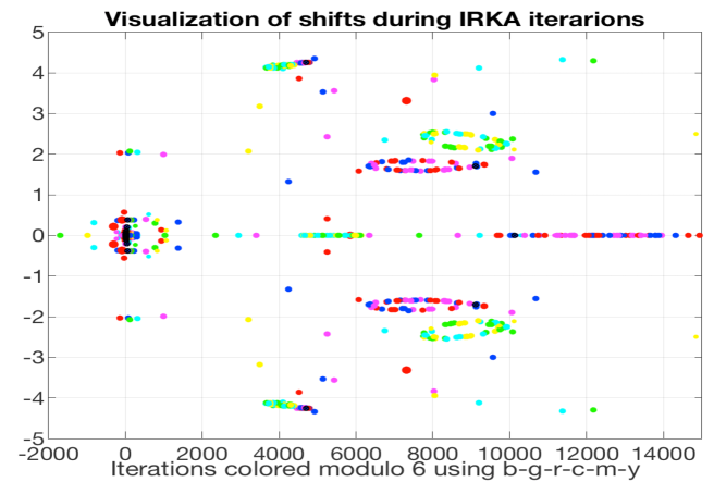
Numerical evidence shows that many scenarios are possible during the iterations in Algorithm 1 – from swift to slow convergence. Characterizing the limit behavior in general is an open problem; in the case of symmetric system local convergence is established in FLAGG2012688 . Moreover, we have also encountered miss–convergence in form of the existence of at least two accumulation points that seem to indicate existence of periodic points of the mapping (24). This is illustrated in the following example.
Example 1
We take the matrix from the CD player benchmark example ChaV2005 ; DraSB92 from the NICONET benchmark collection NICONET and set . With a particular set of initial shifts, we obtained separate behaviours for the odd and the even iterates, as shown in Figure 1.
Hence, it is of both theoretical and practical interest to explore possibilities for improving the convergence. Supplying good initial shift is certainly beneficial, and in DGB-VF-Q-1 ; DGB-VF-Q-2 we show that the less expensive Vector Fitting algorithm can be used for preprocessing/preconditioning to generate good shifts that are then forwarded to IRKA to advance them to a local optimum.
An alternative course of action is to deploy an additional control in the iterations which will keep steering the shifts toward the desired positions. In fact, an example of such an intervention has been already used in the numerical implementation of Algorithm 1. Namely, it can happen that in some steps the matrix (23) is not stable and some of its eigenvalues (24) are in the right half-plane. To correct this situation, the unstable ones (real or complex-conjugate pair(s)) are flipped across the imaginary axis, so that the new shifts stay in the right-half plane.
This is an explicit (brute force) post-festum reassignment of the eigenvalues to correct for stability. In DGB-VF-Q-1 , we showed that such a step (in the framework of Vector Fitting) can be recast as pole placement. Now that we have resorted (implicitly) to the pole placement mechanism, we can think of using it as a proactive strategy for improving convergence. In the rest of this section, we explore this idea and discover interesting connections with some variations of IRKA.
3.2 Reduced input-to-state vector as a pole placement feedback vector
Motivated by the above discussion, we reinterpret (a posteriori) the vector in (23) as the feedback vector that reallocates the eigenvalues444We tacitly assume that throughout the iterations all shifts are simple. of into ; in other words we view (23) as a pole-placement problem. Then we can use the uniqueness argument and write explicitly as (see mehrmann1996app , mehrmann1998cps )
| (25) |
On the other hand, for the fulfillment of the necessary conditions for optimality, besides the Hermite interpolation built in (25), the additional fixed point condition should hold:
| (26) |
The latter is what we hope to reach with the equality in the limit as , and in practice up to a reasonable tolerance, see §4.1. If we consider the condition (26) as an eigenvalue assignment problem, and think of the vector in (23) simply as the feedback vector, then (26) can be satisfied in one step, provided we drop the interpolation condition and use an appropriate feedback vector instead of . The feedback can be constructed explicitly (see mehrmann1996app ; mehrmann1998cps ) as
| (27) |
Of course, the above formula is a special case of (25), where we reflect the poles. However, if at a particular step some of the eigenvalues are unstable, we should not reflect the corresponding shifts. This means that in an implementation, we may apply only partial pole placement. Hence, altogether, it would make sense to interweave interpolation and eigenvalue assignment by combining and using an appropriately chosen parameter , and thus obtain a modified iteration step, as outlined in Algorithm 2. To incorporate this new shift-updating scheme into IRKA, Algorithm 2 should replace Step 8 in Algorithm 1.
Proposition 1
For the real LTI system (1), and closed under complex conjugation, the matrix is similar to a real matrix and, thus, remains closed under complex conjugation.
Proof
From (27), we conclude that is real if is real. Further, if for some , then . We have already concluded that has an analogous structure. Since is real, is similar to a real matrix.
It remains an open problem how to chose the coefficients adaptively and turn Algorithm 2 into a robust black-box scheme. We now show an interesting connection that might provide some guidelines.
3.3 Connection to the Krajewski–Viaro scheme
Improving the convergence of fixed point iterations is an important topic. In general, the fixed point problem can be equivalently solved as the problem
where the parameter is used, e.g., to modify eigenvalues of the corresponding Jacobian. This is a well–known technique (Mann iteration), with many variations. In the context of model reduction, this scheme has been successfully applied by Ferrante, Krajewski, Lepschy and Viarro Ferrante_Krajewski…:1999:Convergent_alg_L2 , and Krajewski and Viaro Krajewski_Viaro:2009:Iterative_Interpolation__alg_L2 . Concretely, Krajewski and Viaro (Krajewski_Viaro:2009:Iterative_Interpolation__alg_L2, , Algorithm 4.) propose a modified step for the IRKA procedure, outlined in Algorithm 3:
| (28) |
Krajewski and Viaro Krajewski_Viaro:2009:Iterative_Interpolation__alg_L2 do not elaborate the details of computing the coefficients of the characteristic polynomials of the reduced matrix . From a numerical point of view, this is not feasible, not even for moderate dimensions. Computing coefficients of the characteristic polynomial by, e.g., the classical Faddeev-Leverrier trace formulas is both too expensive () and too ill-conditioned. A modern approach would reduce the matrix to a Schur or Hessenberg form and then exploit the triangular or, respectively, Hessenberg structure. However, after completing all those (tedious) tasks, the zeros of in Line 4 are best computed by transforming the problem into an eigenvalue computation for an appropriate companion matrix. Ultimately, this approach is only conceptually interesting as a technique for improving convergence, and in this form it is applicable only for small values of .
We now show that when represented in a proper basis, this computation involving characteristic polynomials becomes rather elegant and simple, and further provides interesting insights. In particular, in this proper basis, Algorithm 3 is equivalent to Algorithm 2.
Theorem 3.1
In the Lagrange basis of , the Krajewski–Viaro iteration is equivalent to the “IRKA + pole placement” iteration of Algorithm 2.
Proof
Note that by Lemma 1 we can write , where , , and is the characteristic polynomial of . Further, using Lemma 1, we can write as
If we consider the monic polynomials of degree as the linear manifold , and fix in the Lagrange basis with the nodes , , then
where we used that , and that the feedback vector (27) can be written as
Hence, is the characteristic polynomial of , and we have further
| (29) | |||||
| (30) | |||||
| (31) |
which implies that is the characteristic polynomial of the matrix , represented by the vector from Lines 3 and 4 of Algorithm 2. This follows from the proof of Lemma 1.
Krajewski and Viaro Krajewski_Viaro:2009:Iterative_Interpolation__alg_L2 use a fixed value of the parameter , and show that different (fixed) values may lead to quite different convergence behavior. This modification can turn a non-convergent process into a convergent one, but it can also slow down already convergent one.555We should point out here that the dimensions and are rather small in all reported numerical experiments in Krajewski_Viaro:2009:Iterative_Interpolation__alg_L2 . Following the discussion from Ferrante_Krajewski…:1999:Convergent_alg_L2 , is best chosen to move the smallest eigenvalue of the Jacobian of (evaluated at the fixed point of ) into the interval . This does not seem to be a simple task as it requires estimates of the eigenvalues of the (estimated) Jacobian. Another option is to try different values of in an iterative reduced order model design.
This equivalence of the schemes in Algorithm 2 and in Algorithm 3 reveals a problem that is not easily seen in the framework of Algorithm 3. Now we may clearly see that part of the “energy” in Algorithm 3 is put into reflecting the shifts, and this, at least in some situations, may be wasted effort. Although the optimal reduced order model is guaranteed to be stable, the iterates, generally, are not. This means that some shifts may be in the left–half plane, and the component of the modified will tend to reflect them to the right–half plane. This in turn forces the new reduced matrix to have some eigenvalues in the right–half plane, thus creating a vicious circle. Hence, in the first step (Line 1), one should correct , if necessary.
Remark 1
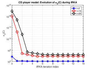
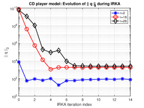
The facts that pole placement may be extremely ill-conditioned he:ppp , where (depending on the distribution of the target values) plenty may be even as small as , and that IRKA is actually doing pole placement in disguise, open many nontrivial issues. For instance, what is a reasonable threshold for the stopping criterion? Will we be able to actually test it (and detect convergence) in finite precision computation? What are relevant condition numbers in the overall process? Do IRKA iterations drive the shifts to well-conditioned configurations for which the feedback vector (the reduced input) is reasonably small (in norm, as illustrated in the right panels of Figure 2 and Figure 3 in Example 2 below) and successful in achieving numerical convergence? If yes, what is the underlying principle/driving mechanism? In the next section, we touch upon some of these issues.
4 Perturbation effects and backward stability in IRKA
We turn our attention now to numerical considerations in the implementation of IRKA. We focus on two issues: (i) What are the perturbative effects of finite-precision arithmetic in terms of system-theoretic quantities? (ii) What are the effects of “numerical convergence” on the reduced model?
4.1 Limitations of finite precision arithmetic
Suppose that we are given magic shifts so that the eigenvalues of are exactly , or up to a small tolerance . However, in floating point computations, the vector is computed up to an error , and therefore instead of , we have . In practice, the source of is twofold: First, in large-scale settings, the primitive Krylov bases and are usually computed by an iterative method which uses restricted information from suitably chosen subspaces and thus generates a truncation error; see, e.g., beattie2012inexact ; ahuja2012recycling ; ahuja2015recycling . In addition, computation is polluted by omnipresent rounding errors of finite precision arithmetic. How the size of influences the other components of the IRKA is a relevant information that we investigate in this subsection.
Assume for the moment that is the only perturbation in one step of IRKA. We want to understand how the eigenvalues of and differ as a function of . In particular, we want to reveal the relevant condition numbers that play a role in this perturbation analysis.
Theorem 4.1
Let and be diagonalizable, where . Let and have the spectral decompositions and , where , and the eigenvector matrices and as described in Corollary 1. Then there exists a permutation such that
| (32) |
Proof
Note that we can equivalently compare the spectra of and . From (17), we know that the spectral decomposition of is given by
| (33) |
Similarly for , we obtain
| (34) |
Next we employ the perturbation results of Elsner and Friedland elsner1995svd , and Eisenstat and Ipsen eisenstat1998tap , while taking into account the special structure of both matrices. Write , where . Using the spectral decompositions (22) and (34), the matrix can be transformed into
| (35) |
Set and take the absolute value of , an arbitrary entry of at the th position, to obtain
Hence
where the Hadamard product matrix is entry–wise bounded by
where is a doubly–stochastic matrix; see elsner1995svd . Hence
| (36) |
The expression on the left–hand side of (36) can be considered as a function defined on the convex polyhedral set of doubly–stochastic matrices, whose extreme points are the permutation matrices. Thus, for some permutation , we obtain
Then, using (22), the spectral decomposition of , and the definition of complete the proof.
Remark 2
One can write (35) as and conclude that there exists a permutation such that (see elsner1995svd )
Remark 3
The right–hand side in relation (32) can also be bounded by
From the numerical point of view, Theorem 4.1 cannot be good news – Cauchy matrices can be ill–conditioned. A few random trials will quickly produce a Cauchy matrix with condition number greater than . The most notorious example is the Hilbert matrix, which at the dimension has a condition number larger than . No function of the matrix that is influenced by that condition number of the eigenvectors can be satisfactorily computed in bit machine arithmetic. The bit double precision allows only slightly larger dimensions before the condition number takes over the machine double precision.
On the other hand, we note that our goal is not to place the shifts at any predefined locations in the complex plane. Instead, we are willing to let them go wherever they want, under the condition that they remain closed under conjugation and stationary at those positions. It should also be noted that the distribution of the shifts obviously plays a role in this considerations. The following example will illustrate this; especially the impact of the optimal interpolation points.
Example 2
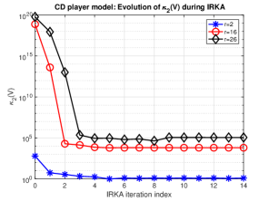
As in Example 1, we first take the CD player model ChaV2005 ; DraSB92 of order and apply IRKA as in Algorithm 1 for , , and . In each case, IRKA is initialized by randomly assigned shifts. The condition numbers of for each case, recorded throughout the iterations, are shown on the left panel of Figure 2. IRKA drastically reduces the condition number of throughout the iteration, more than order of magnitudes for and cases. Therefore, IRKA keeps assigning shifts in such a way that becomes better and better conditioned; thus in affect limiting the perturbation effects predicted by Theorem 4.1. Moreover, we can observe that the reduced input vectors , which act also as feedback vectors that steer the shifts, diminish in norm over the iterations; see the right panel of Figure 2.
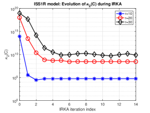
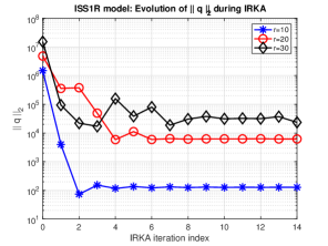
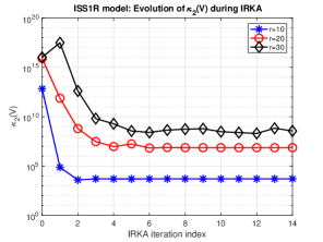
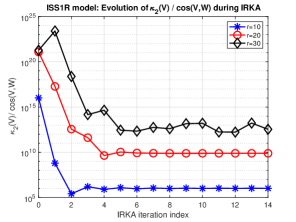
We have observed the same effect in all the examples we have tried. For brevity, we include only one more such result using the International Space Station 1R Module morGugAB01 ; antoulas2001asurvey of order . As for the CD Player model, we reduce this model with IRKA using random initial shifts and this time chose reduced orders of , , and . The results depicted in Figure 3 reveal the same behavior: The condition number is reduced significantly during IRKA as shifts converge to the optimal shifts; the same holds for the reduced input norms . These observation raises intriguing theoretical questions about the distribution of the -optimal shifts, as their impact mimics that of Chebyshev points (as opposed to linearly spaced ones) in polynomial interpolation. These issues will not be studied here and are left to future papers.
4.2 Stopping criterion and backward stability
Analytically, optimality is satisfied when . However, in practice Algorithm 1 will be terminated once a numerical convergence threshold is met. In this section, we will investigate the impact of numerical convergence on the resulting reduced model. The pole-placement connection we established in Section 3 will play a fundamental role in answering this question.
Suppose that in Algorithm 1 a numerical stopping (convergence) criterion has been satisfied, i.e., the eigenvalues of are close to the reflected shifts. Both the shifts and the computed eigenvalues are unordered –tuples of complex numbers, and we measure their distance using optimal matching, see §3.1. Hence, we define the indexing of so that
Recall that the shifts are closed under conjugation, with strictly positive real parts, and all assumed to be simple. The eigenvalues are assumed also simple, and they are obviously closed under conjugation. With this setup, we write
| (37) |
where we note that the ’s are closed under conjugation as well. Our goal is to relate the ’s and the quality of the computed reduced order model identified by the triplet in the sense of backward error. In particular, we need a yardstick to determine when an is small.
There is a caveat here: for given shifts , the vector consists of the computed eigenvalues, thus possibly highly ill–conditioned and computed with large errors. Our analysis here considers the computed eigenvalues as exact but for a slightly changed input data,666This is the classical backward error interpretation. and we focus on the stopping criterion and how to justify it through a backward stability statement. This means that we want to interpret the computed reduced order model as an exact reduced order model for an LTI close to the original one (1).
The representation of the reduced order model in the primitive basis presented in Section 2 yields an elegant structure and provides theoretical insights. On the other hand, having numerical computation in mind, the same structure gives reasons to exercise caution. This caution is particularly justified because, as we showed in Section 3, the ultimate step of the iteration is an eigenvalue assignment problem: find the shifts such that the eigenvalues of are the reflected shifts.
Using (25), (37), and Lemma 1, we know that the vector satisfies
| (38) |
We now do the following Gedankenexperiment. Consider the true reflections of the shifts, . Since the pair is controllable777Let and . Then, the pair is called controllable if , there exists such that the eigenvalues of are precisely . In fact, by the formula (27), the feedback is explicitly given as
| (39) |
Comparing (38) and (39), we see that our computed vector satisfies
| (40) |
Since all the shifts are in the right–half–plane, is bounded from below by . We find it desirable to have our actually computed close to , because does exactly what we would like the computed to achieve in the limit. This indicates one possible stopping criterion for the iterations – the maximal allowed distance between the new and the old shifts should guarantee small for all .
If we define , then its eigenvalues are the reflections of the shifts. Comparing this outcome with the actually computed , we obtain the following result.
Proposition 2
Let Algorithm 1 be stopped with computed , and let the eigenvalues of be , . Let
| (41) |
Then there exists with eigenvalues , and such that ; , ; and
| (42) |
Proof
Define using (39) and write . Write the actually computed reduced matrix as
| (43) |
Note that . Further, using and taking the norm we get
and thus the norm of can be estimated as
completing the proof.
Remark 4
We conclude that in the vicinity of our computed data (reduced quantities) and , there exist and that satisfy the stopping criterion exactly. Both and are estimated by the size of . But there is a subtlety here: we cannot use as the stopping criterion. In other words, if we compute and conclude that is small, it does not mean that the ’s are close to the reflections of the ’s. There is difference between continuity and forward stability.
Our next goal is to interpret and as the results of backward perturbations in the initial data , .
Theorem 4.2
Under the assumptions of Proposition 2, there exist backward perturbations and such that the reduced order system
corresponds to exact model reduction of the perturbed full-order model described by the triplet of matrices and has its poles at the reflected shifts. Let and denote the transfer functions of this reduced order system, and the backward perturbed original system, respectively. Then, , . The backward perturbations satisfy
| (44) |
and
| (45) |
where and .
Proof
First, recall that , where . Since has full row–rank, we can determine such that . (The unique of minimal Euclidean norm is .) Using (43) and we can write then
| (46) |
where . Since we can express as with smallest possible , we obtain
| (47) |
Set and note that . From Proposition 2, under the mild assumption that , we conclude that
Since and , we have
Further, it holds that
and this implicitly enforces the interpolation conditions.
Remark 5
To claim Hermite interpolation, the only freedom left is to change into to guarantee that for . In other words, with some matrix , we should have
If commutes with , then . We can take and instead of the equality (which is not possible to to obtain), we can choose , which is the least squares approximation. Even though this least-squares construction might provide a near-Hermite interpolation, a more elaborate construction is needed to obtain exact Hermite interpolation for a backward perturbed system. The framework that Beattie et al. beattie2012inexact provided for Hermite interpolation of a backward perturbed system in the special case of inexact solves might prove helpful in this direction.
Our analysis in Section 4.1, specifically Theorem 4.1, illustrated that the condition number of the Cauchy matrix plays a crucial role in the perturbation analysis. And the numerical examples showed that despite Cauchy matrices are known to be extremely ill-conditioned, the IRKA iterations drastically reduced these conditions numbers as the shifts converge to the optimal ones, i.e., as IRKA converges. Our analysis in this section now reveals another important quantity measure: . Next, we will repeat the same numerical examples of Section 4.1 and inspect how and vary during IRKA.
Example 3
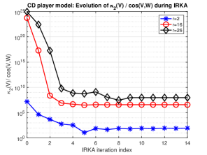
We use the same models and experiments from Example 2. During the reduction of the CD player model to , , and via IRKA, we record the evolution of and . The results depicted in Figure 4 show a similar story: Both quantities are drastically reduced during the iteration and thus leading to significantly smaller backward errors and in Theorem 4.2.
We repeat the same experiments for the ISS 1R model and the results are shown in Figure 5. The conclusion is the same: and are reduced ten orders of magnitudes during IRKA.
5 Conclusions
By employing primitive rational Krylov bases, we have provided here an analysis for the structure of reduced order quantities appearing in IRKA that reveals a deep connection to the classic pole-placement problem. We exploited this connection to motivate algorithmic modifications to IRKA and developed a complementary backward stability analysis. Several numerical examples demonstrate IRKA’s remarkable tendency to realign shifts (interpolation points) in a way that drastically reduces the condition numbers of the quantities involved, thus minimizing perturbative effects and accounting in some measure for IRKA’s observed robustness.
References
- (1) Ahuja, K., Benner, P., de Sturler, E., Feng, L.: Recycling bicgstab with an application to parametric model order reduction. SIAM Journal on Scientific Computing 37(5), S429–S446 (2015)
- (2) Ahuja, K., de Sturler, E., Gugercin, S., Chang, E.: Recycling BiCG with an application to model reduction. SIAM Journal on Scientific Computing 34(4), A1925–A1949 (2012)
- (3) Antoulas, A., , Beattie, C., Gugercin, S.: Interpolatory Methods for Model Reduction. Society for Industrial and Applied Mathematics, to appear (2020)
- (4) Antoulas, A.: Approximation of Large-Scale Dynamical Systems (Advances in Design and Control). Society for Industrial and Applied Mathematics, Philadelphia, PA, USA (2005)
- (5) Antoulas, A.C., Beattie, C.A., Gugercin, S.: Interpolatory model reduction of large-scale dynamical systems. In: J. Mohammadpour, K. Grigoriadis (eds.) Efficient Modeling and Control of Large-Scale Systems, pp. 2–58. Springer-Verlag (2010)
- (6) Antoulas, A.C., Sorensen, D.C., Gugercin, S.: A survey of model reduction methods for large-scale systems. Contemporary Mathematics 280, 193–219 (2001)
- (7) Beattie, C., Gugercin, S.: Krylov-based minimization for optimal model reduction. In: Proceedings of 46th IEEE Conference on Decision and Control, pp. 4385–4390 (2007)
- (8) Beattie, C., Gugercin, S.: A trust region method for optimal model reduction. In: Proceedings of 48th IEEE Conference on Decision and Control, pp. 5370–5375 (2009)
- (9) Beattie, C., Gugercin, S.: Realization-independent -approximation. In: Proceedings of 51st IEEE Conference on Decision and Control, pp. 4953 – 4958 (2012)
- (10) Beattie, C., Gugercin, S., Wyatt, S.: Inexact solves in interpolatory model reduction. Linear Algebra and its Applications 436(8), 2916–2943 (2012)
- (11) Benner, P., Breiten, T.: Interpolation-based -model reduction of bilinear control systems. SIAM J. Matrix Anal. Appl. 33, 859–885 (2012)
- (12) Benner, P., Goyal, P., Gugercin, S.: -quasi-optimal model order reduction for quadratic-bilinear control systems. SIAM Journal on Matrix Analysis and Applications 39(2), 983–1032 (2018)
- (13) Benner, P., Köhler, M., Saak, J.: Sparse-dense Sylvester equations in -model order reduction. Tech. Rep. MPIMD/11-11, Max Planck Institute Magdeburg Preprints (2011)
- (14) Benner, P., Ohlberger, M., Cohen, A., Willcox, K.: Model Reduction and Approximation. Society for Industrial and Applied Mathematics, Philadelphia, PA (2017). DOI 10.1137/1.9781611974829. URL https://epubs.siam.org/doi/abs/10.1137/1.9781611974829
- (15) Breiten, T., Beattie, C., Gugercin, S.: Near-optimal frequency-weighted interpolatory model reduction. Systems & Control Letters 78, 8–18 (2015)
- (16) Bunse-Gerstner, A., Kubalinska, D., Vossen, G., Wilczek, D.: -optimal model reduction for large scale discrete dynamical MIMO systems. Journal of Computational and Applied Mathematics (2009). Doi:10.1016/j.cam.2008.12.029
- (17) Chahlaoui, Y., Dooren, P.V.: A collection of benchmark examples for model reduction of linear time invariant dynamical systems. Tech. rep., SLICOT Working Note 2002-2 (2002)
- (18) Chahlaoui, Y., Van Dooren, P.: Benchmark examples for model reduction of linear time-invariant dynamical systems. In: P. Benner, D. Sorensen, V. Mehrmann (eds.) Dimension Reduction of Large-Scale Systems, pp. 379–392. Springer Berlin Heidelberg, Berlin, Heidelberg (2005)
- (19) Draijer, W., Steinbuch, M., Bosgra, O.: Adaptive control of the radial servo system of a compact disc player. Automatica 28(3), 455–462 (1992). DOI 10.1016/0005-1098(92)90171-B
- (20) Drmač, Z., Gugercin, S., Beattie, C.: Quadrature-based vector fitting for discretized approximation. SIAM Journal on Scientific Computing 37(2), A625–A652 (2015). DOI 10.1137/140961511. URL https://doi.org/10.1137/140961511
- (21) Drmač, Z., Gugercin, S., Beattie, C.: Vector fitting for matrix-valued rational approximation. SIAM Journal on Scientific Computing 37(5), A2346–A2379 (2015). DOI 10.1137/15M1010774. URL https://doi.org/10.1137/15M1010774
- (22) Eisenstat, S., Ipsen, I.: Three Absolute Perturbation Bounds for Matrix Eigenvalues Imply Relative Bounds. SIAM J. Matrix Anal. Appl. 20, 149 (1998)
- (23) Elsner, L., Friedland, S.: Singular Values Doubly Stochastic Matrices and Applications. Linear Algebra and its Applications 220(1), 161–170 (1995)
- (24) Ferrante, A., Krajewski, W., Lepschy, A., Viaro, U.: Convergent algorithm for model reduction. Automatica 35, 75–79 (1999)
- (25) Flagg, G., C., B., Gugercin, S.: Convergence of the iterative rational krylov algorithm. Systems & Control Letters 61(6), 688 – 691 (2012). DOI https://doi.org/10.1016/j.sysconle.2012.03.005. URL http://www.sciencedirect.com/science/article/pii/S0167691112000576
- (26) Flagg, G., Gugercin, S.: Multipoint Volterra series interpolation and optimal model reduction of bilinear systems. SIAM Journal on Matrix Analysis and Applications 36, 549–579 (2015)
- (27) Goyal, P., Redmann, M.: Time-limited h2-optimal model order reduction. Applied Mathematics and Computation 355, 184–197 (2019)
- (28) Gugercin, S.: An iterative SVD-Krylov based method for model reduction of large-scale dynamical systems. Linear Algebra and Its Applications 428(8-9), 1964–1986 (2008)
- (29) Gugercin, S., Antoulas, A.C., Beattie, C.: model reduction for large-scale linear dynamical systems. SIAM J. Matrix Anal. Appl. 30, 609–638 (2008). DOI 10.1137/060666123. URL http://portal.acm.org/citation.cfm?id=1461865.1461876
- (30) Gugercin, S., Antoulas, A.C., Bedrossian, M.: Approximation of the international space station 1r and 12a flex models. In: Proceedings of the IEEE Conference on Decision and Control, pp. 1515–1516 (2001). DOI 10.1109/CDC.2001.981109
- (31) He, C., Laub, A., Mehrmann, V.: Placing plenty of poles is pretty preposterous. Tech. rep., Preprint SPC 95-17, Forschergruppe Scientific Parallel Computing, Fakultät für Mathematik, TU Chemnitz-Zwickau http://www.tu-chemnitz.de/sfb393/Files/AFS/spc95_17.ps.Z (1995)
- (32) Hokanson, J., Magruder, C.: -optimal model reduction using projected nonlinear least squares (1811.11962) (2018). URL https://arxiv.org/abs/1811.11962
- (33) Hyland, D., Bernstein, D.: The optimal projection equations for model reduction and the relationships among the methods of Wilson, Skelton, and Moore. IEEE Transactions on Automatic Control, 30(12), 1201–1211 (1985)
- (34) Krajewski, W., Lepschy, A., Redivo-Zaglia, M., Viaro, U.: A program for solving the reduced-order model problem with fixed denominator degree. Numerical Algorithms 9(2), 355–377 (1995)
- (35) Krajewski, W., Viaro, U.: Iterative–interpolation algorithms for model reduction. Control and Cybernetics 38(2), 543–554 (2009)
- (36) Mehrmann, V., Xu, H.: An analysis of the pole placement problem. I. the single-input case. Electronic Transactions on Numerical Analysis 4, 89–105 (1996)
- (37) Mehrmann, V., Xu, H.: Choosing poles so that the single-input pole placement problem is well conditioned. SIAM J. Matrix Anal. Appl. 19(3), 664–681 (1998)
- (38) Meier III, L., Luenberger, D.: Approximation of linear constant systems. Automatic Control, IEEE Transactions on 12(5), 585–588 (1967)
- (39) Panzer, H., Jaensch, S., Wolf, T., Lohmann, B.: A greedy rational Krylov method for -pseudooptimal model order reduction with preservation of stability. In: American Control Conference, 2013, pp. 5512–5517 (2013)
- (40) Poussot-Vassal, C.: An iterative svd-tangential interpolation method for medium-scale mimo systems approximation with application on flexible aircraft. In: 2011 50th IEEE Conference on Decision and Control and European Control Conference, pp. 7117–7122. IEEE (2011)
- (41) Spanos, J., Milman, M., Mingori, D.: A new algorithm for optimal model reduction. Automatica 28(5), 897–909 (1992)
- (42) Van Dooren, P., Gallivan, K., Absil, P.: -optimal model reduction of MIMO systems. Applied Mathematics Letters 21(12), 1267–1273 (2008)
- (43) Vuillemin, P., Poussot-Vassal, C., Alazard, D.: optimal and frequency limited approximation methods for large-scale LTI dynamical systems. IFAC Proceedings Volumes 46(2), 719–724 (2013)
- (44) Žigić, D., Watson, L., Beattie, C.: Contragredient transformations applied to the optimal projection equations. Linear Algebra and Its Applications 188, 665–676 (1993)
- (45) Wilson, D.: Optimum solution of model-reduction problem. Proc. IEE 117(6), 1161–1165 (1970)
- (46) Xu, Y., Zeng, T.: Optimal model reduction for large scale MIMO systems via tangential interpolation. International Journal of Numerical Analysis and Modeling 8(1), 174–188 (2011)