AI-optimized detector design for the future
Electron-Ion Collider: the dual-radiator RICH case
Abstract
Advanced detector R&D requires performing computationally intensive and detailed simulations as part of the detector-design optimization process. We propose a general approach to this process based on Bayesian optimization and machine learning that encodes detector requirements. As a case study, we focus on the design of the dual-radiator Ring Imaging Cherenkov (dRICH) detector under development as a potential component of the particle-identification system at the future Electron-Ion Collider (EIC). The EIC is a US-led frontier accelerator project for nuclear physics, which has been proposed to further explore the structure and interactions of nuclear matter at the scale of sea quarks and gluons. We show that the detector design obtained with our automated and highly parallelized framework outperforms the baseline dRICH design within the assumptions of the current model. Our approach can be applied to any detector R&D, provided that realistic simulations are available.
1 Introduction
Applications of methods based on Artificial Intelligence (AI) are becoming ubiquitous in all areas of our society; in particle and nuclear physics in particular, detector Research and Development (R&D) can certainly benefit from AI and this manuscript provides an explicit example of its usefulness.
In this paper we propose a general approach based on Bayesian optimization (BO) [1, 2] to optimize the design of any detector starting from its R&D phase. BO is particularly useful for global optimization of black-box functions that can be noisy and non-differentiable. The BO approach allows to encode detector requirements like mechanical and geometrical constraints and efficiently maximize a suitable figure of merit used to improve the detector design. We apply this general method to a specific use-case: the design of the dual-radiator Ring Imaging Cherenkov (dRICH) detector within the current Electron-Ion Collider (EIC) large scale initiative.
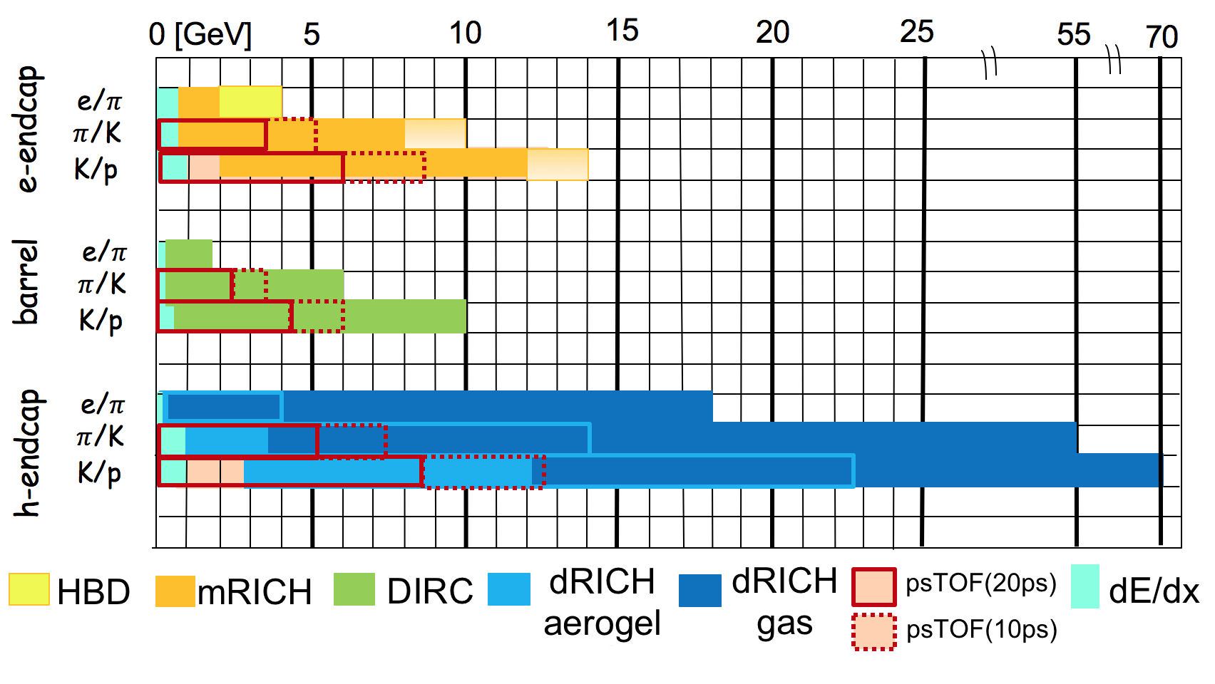
The future EIC [3, 4] will be a unique experimental facility that will open up new frontiers for exploring Quantum Chromodynamics (QCD), e.g. the 3D structure of nucleons and nuclei in terms of quarks and gluons, and the behaviour of nuclear matter at unprecedented saturated gluon densities. A key challenge for EIC detectors involves particle identification (PID)—especially hadron identification—which is required for studying many of the most important experimental processes at the EIC. For example, the simulated phase space for pions and kaons in deep inelastic scattering (DIS) processes shows the need for hadronic PID over a momentum range up to 50 GeV/c in the hadron endcap, up to 10 GeV/c in the electron endcap, and up to 5–7 GeV/c in the central barrel [5].
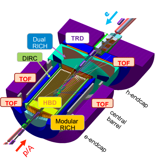
The purpose of the EIC-PID consortium is to develop an integrated PID system that satisfies the requirements imposed by the EIC science program. The current baseline design of the EIC-PID system, shown in Fig. 1, includes the dRICH and a modular-aerogel RICH (mRICH) that uses a Fresnel lens placed in the electron endcap [6, 7]. In addition, the Detection of Internally Reflected Cherenkov light (DIRC) detector [8] is located in the barrel region, where a fast time-of-flight (TOF) system is foreseen to provide PID for low-momenta particles.
In what follows we show that the new dRICH detector design obtained with our automated and highly parallelized framework based on BO outperforms the baseline dRICH design within the assumptions of the present simulated model.111Throughout this article, we refer to the dRICH design prior to this work [6], as the baseline design.
2 Dual-radiator RICH
The goal of the dRICH detector is to provide full hadron identification (/K/p better than apart) from a few GeV/c up to 50 GeV/c in the (outgoing) ion-side endcap of the EIC detector (see Fig. 1), covering polar angles up to 25 degrees; it will also offer e/ separation up to about 15 GeV/c as a byproduct [6]. The dRICH concept was inspired by the HERMES [10] and LHCb (RICH1 in Run 1) [11, 12] dual-radiator RICH detectors. The baseline design (see Fig. 2) consists of a large conical-trunk tank (160 cm height, 180220 cm radii) divided into 6 identical, open, sectors (petals); the tank contains an aerogel radiator at the entrance and is filled by C2F6 gas acting as a second radiator. The photons from both radiators share the same outward-focusing spherical mirror and highly segmented (3 mm2 pixel size) photosensors located outside of the charged-particle acceptance. The baseline configuration is the result of simulation analyses taking into account the geometrical and physical constraints; it can be summarized by the following key parameters: i) maximum device length 1.65 m; ii) aerogel radiator refractive index n(400 nm) = 1.02 and thickness 4 cm; iii) C2F6 gas tank length 1.6 m; iv) polar angle coverage ; v) mirror radius 2.9 m.
In this study, we benefited from the experience of several groups that have built similar devices in the past [10, 12, 13, 14], and also from the CLAS12 RICH work which is in progress [15]. The dRICH baseline detector (see Fig. 2) has been simulated within a Geant4/GEMC framework [16]. The Geant4 simulation is based on realistic optical properties of aerogels tested and characterized by the CLAS12 RICH collaboration [15, 17]. Absorption length and Rayleigh scattering are included in the simulation, the latter being one of the main sources of background, along with optical dispersion; the spectrum of the Rayleigh scattering is , hence this contribution becomes relevant for photon wavelengths below nm.222The 300 nm value is the safe, approximate, cut-off coming out from the HERMES [10] and LHCb [11] studies for their dual-radiator RICHes, where 290 nm and 300 nm have been adopted respectively. The choice of the cut-off is also influenced by the specific dispersion relation of the aerogel; its final value in dRICH will depend from the prototyping outcomes, the aerogel characterization, and likely the application of the optimization method described here.
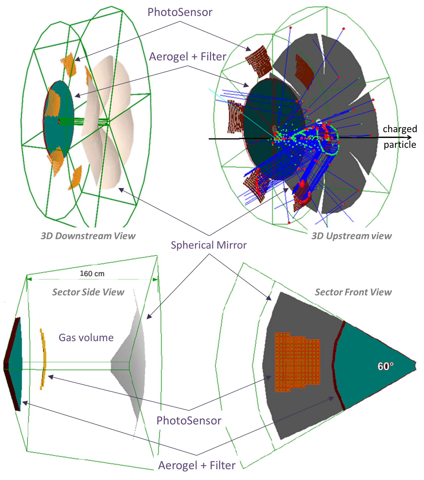
Photons produced in the aerogel with wavelengths below 300 nm are removed, imitating the effects of an acrylic filter that will separate the aerogel from the gas, for both filtering and avoiding chemical degradation of the aerogel. The mirror reflectivity is assumed to be 95% and uniform. The dRICH is in a non-negligible magnetic field and the charged-particle tracks are bending as they pass through the Cherenkov radiators, providing an additional source of uncertainty in the Cherenkov ring reconstruction. The size of this effect is proportional to the path length within the Cherenkov radiators, and therefore, it is important for gas radiator. The magnetic field used in the simulation is that of the JLab detector design at 3T central field.333The solenoid is still under development and its central magnetic field is now expected to be smaller than 3 T. This value is, therefore, conservative for the dRICH simulation results. The impact of the magnetic field is confined to the gas angular resolution at large polar angle (right plot of Fig. 3). Our proposed optimization method and its applicability do not depend on the strength of the magnetic field. The optical sensor area in such a mirror-focusing design can be rather compact, and can be placed in the shadow of a barrel calorimeter, outside of the radiator acceptance. The pixel size of the photosensors has been assumed to be 3 mm; the quantum efficiency curve of the multi-anode PMT Hamamatsu-H12700-03 [18] has also been assumed, which is similar to that of any potential photosensor suitable for sustaining both relatively high magnetic field and irradiation expected in the dRICH detection region.
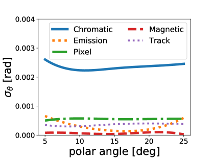
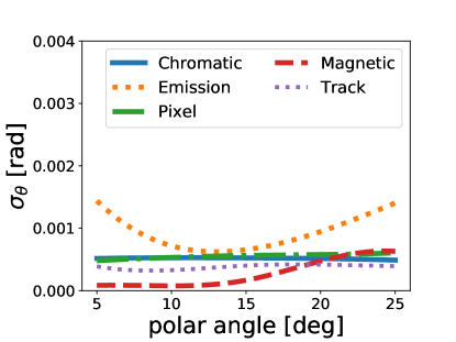
The reconstruction of the Cherenkov angles from either aerogel or gas photons coming from the single particle simulated per event is based on the Inverse Ray Tracing algorithm used by the HERMES experiment (see Ref. [10] for details on the algorithm).444The large separation of the Cherenkov photon emission angles in aerogel (12 deg) and gas (2 deg) makes in practice straightforward the association of the photons hits to the correct radiator. Figure 3 shows the main error contributions to the single photoelectron (p.e.) angular resolution of the two radiators as a function of the charged particle polar angle, see also appendix A and Ref. [6].
In addition to the angular error, the ring reconstruction is affected by the level of noise, whose main sources are: i) the aforementioned aerogel scattered photons which are largely suppressed by a high-pass wavelength filter assumed at 300 nm; this is included in the simulation; ii) the intrinsic noise of the sensors and electronics which is simulated as random uniform noise (30 hit/event) in the whole detector area;555The dRICH sensor and electronics are not defined yet; one can estimate their impact assuming typical performance of current state of the art systems. With 1 kHz sensor dark count rate, in a conventional 100 ns gated triggered electronics (recent, higher performance, solutions such as streaming readout are expected to be adopted in the final design, the EIC-eRD23 [19] is devoted to this specific topic) we expect a modest 5 random noisy hit/event/sector, that corresponds to about 3 noisy hits in the aerogel ring area. iii) the physics background related to the event particle multiplicity which is related to the wide EIC physics phenomenology, and is not included in the current simulation.666The current dRICH development stage is focused on the physical-optical properties of the detector which mainly depend on the expected average phase space of the hadrons. In 2019 the dRICH R&D entered the prototyping phase that, in the coming years, will validate the above described Monte Carlo model and eventually fine-tune the implemented simulator.
3 Methodology and Analysis
Determining how much space to allocate for various detector components, what kind of sensors to use, and which configuration provides the best performance, are often dilemmas that need to be resolved without increasing costs. In addition, for multipurpose experiments like the EIC, optimizing the detector design requires performing large-scale simulations of many important physics processes. Therefore, learning algorithms (e.g., AI-based) can potentially produce better designs while using less resources. Nowadays there are many AI-based global optimization procedures (e.g. reinforcement learning, evolutionary algorithm). Among these learning algorithms, the above mentioned BOs have become popular as they are able to perform global optimization of black-box functions, which can be noisy and non-differentiable. These features make BOs particularly well suited for optimizing the EIC detector design, and, in general, BOs could potentially be deployed for a variety of critical R&D efforts in the near future.
BOs search for the global optimum over a bounded domain of black-box functions, formally expressed as .777Here, we assume one is searching for a global minimum. The aim of a BO is to keep the number of iterations required to identify the optimal value relatively small. The BO approach has been applied to solve a wide range of problems in different areas from robotics to deep learning [20, 21, 22, 23, 24, 25, 26]. For example, in experimental particle physics it has been used to tune the parameters of Monte Carlo generators [27]. When applied to detector design, each point explored corresponds to a different detector configuration (design point). The function can be thought of as a figure of merit that has to be optimized (e.g., a proxy of the PID performance). Typically Gaussian processes [28] (GP) are used to build a surrogate model of , but other regression methods, such as decision trees, can also be used. For example, Gradient Boosted Regression Trees (GBRT) is a flexible non-parametric statistical learning technique used to model very-expensive-to-evaluate functions. The model is improved by sequentially evaluating the expensive function at the next candidate detector configurations, thereby finding the minimum with as few evaluations as possible. A cheap utility function is considered, called the acquisition function, that guides the process of deciding the next points to evaluate. The utility function should balance the trade-off of exploiting the regions near the current optimal solution, and exploring regions where the probabilistic model is highly uncertain.
We have explored the use of BOs in the optimization of the design of the dRICH. Each point in the parameter space corresponds to a different detector design, and consists of a vector of values for the parameters in the Table 1. Running the Geant4 simulation and subsequent analysis of a single detector design point takes about 10 minutes on a single physical core.888Model name: Intel(R) Xeon(R) CPU E5-2697 v4 @ 2.30GHz, two threads are run per core. A grid search with just 8 dimensions even run on 50 cores in parallel looks unfeasible due to the “curse of dimensionality” [29]. Several open-source tools are available for Bayesian optimization (see, e.g., Ref. [2]); the results shown in the following are based on the scikit-learn package [30].
In this work, eight parameters are considered when optimizing the dRICH design, inspired by the previous studies done in Ref. [6]: the refractive index and thickness of the aerogel radiator; the focusing mirror radius, its longitudinal (which determines the effective thickness of the gas along the beam direction) and radial positions (corresponding to the axis going in the radial direction in each of the six mirror sectors, see Fig. 2); and the 3D shifts of the photon sensor tiles with respect to the mirror center on a spherical surface, which contribute to determine the sensor area and orientation relative to the mirror.999 The Cartesian reference frame of the tile shifts has the origin in the center of a dRICH conical-trunk sector (see Fig. 2), is along the beam, along the sector radii, and derived accordingly; the single sector detector is then replicated six times to build the whole detector (namely, a standard Geant4 procedure).
These parameters, reported in Table 1, cover rather exhaustively the two major components of the dRICH: its radiators and optics.
They have been chosen to improve the dRICH PID performance,
under the constraint that it is possible to implement any values resulting from the optimization with (at worst) only minor hardware issues to solve. We assume 100 as the minimum feasible tolerance on each spatial alignment parameter, whereas for the aerogel, we assume 1 on the thickness and 0.2% on the refractive index.
A relevant parameter has been essentially neglected in the optimization: the gas refractive index, whose tuning would require a pressurized detector making this choice hardly convenient.
We also postpone the optimization of the TOF-aerogel transition region, since at the moment these are two separate detectors with different simulation frameworks.
The parameter space can be extended once detailed results from prototyping and tests will be available.
| parameter | description | range [units] | tolerance [units] |
|---|---|---|---|
| R | mirror radius | [290,300] [cm] | 100 [m] |
| pos r | radial position of mirror center | [125,140] [cm] | 100 [m] |
| pos l | longitudinal position of mirror center | [-305,-295] [cm] | 100 [m] |
| tiles x | shift along x of tiles center | [-5,5] [cm] | 100 [m] |
| tiles y | shift along y of tiles center | [-5,5] [cm] | 100 [m] |
| tiles z | shift along z of tiles center | [-105,-95] [cm] | 100 [m] |
| n | aerogel refractive index | [1.015,1.030] | 0.2% |
| t | aerogel thickness | [3.0,6.0] [cm] | 1 [mm] |
Since the aim of the design optimization is to maximize the PID performance of the dRICH, it is natural to build the objective function using the separation power between pions and kaons, defined as
| (3.1) |
where and are the mean Cherenkov angles for kaons and pions, respectively, obtained from the angular distributions reconstructed by Inverse Ray Tracing [10]. Here, is the mean number of detected photo-electrons and the single photo-electron angular resolution; the reconstructed angles are approximately Gaussian distributed, hence corresponds to the averaged RMS of the above mean angles, i.e. the ring angular resolution.
In order to simultaneously optimize the combined PID performance of both the aerogel and gas parts in the dRICH, two working points have been chosen based on the performance of the baseline design. In particular, we chose one momentum value with separation each for the aerogel and the gas: 14 GeV/c and 60 GeV/c, each close to the end of the curves reported in Fig. 3 for the aerogel and gas, respectively. The goal here is to optimize the quantities ()1,2 corresponding to the working points and . One choice of the figure of merit which proved to be effective is the harmonic mean
| (3.2) |
The harmonic mean tends to favor the case where the PID performance (i.e. ) is high in both parts of the detector.
The optimization consists of finding the maximum of the figure of merit (FoM), as defined in (3.2).101010BOs in skopt search for a minimum, hence we change the sign of (3.2).
Samples of pions and kaons have been produced with Geant4 [16] using particle guns with central values of the momentum corresponding to 14 and 60 GeV/c.
In order to cover a larger region of the phase-space in the forward sector of the detector, the polar angles have been spanned uniformly from 5 to 15 degrees.
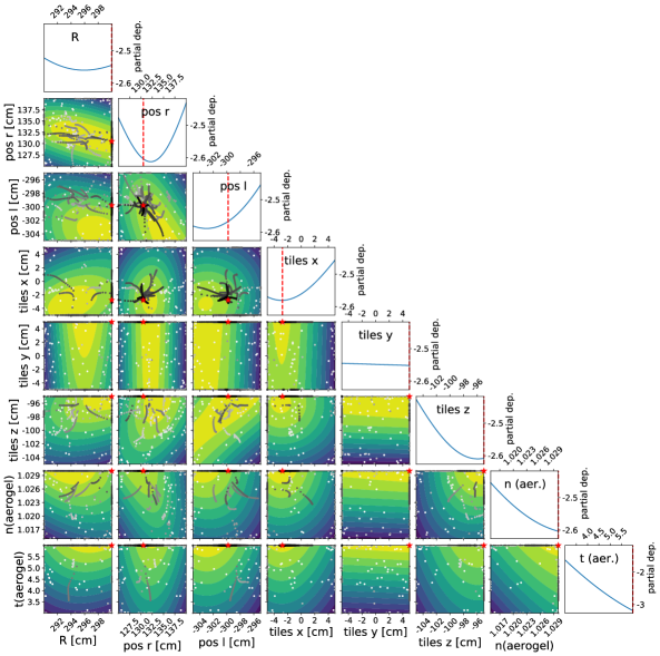
Figure 4 shows the posterior distribution after calls projected in 2-dimensional subspaces of the design parameter space. These plots illustrate the possible correlations among the parameters. The optimal point in each subspace is marked with a red star. Notice that the black points, corresponding to the points evaluated by the BO in its ask-and-tell procedure, tend to form basins of attraction around the minimum. Recall that the black-box function we are optimizing is noisy in the Geant4 simulation (see also Appendix B for a detailed study on statistical uncertainties). Plots of the partial dependence of the objective function on each parameter are displayed in Fig. 4. Given a function of variables, the partial dependence of on the -th variable is defined as [31]
| (3.3) |
The above sum runs over a set of random points from the search space, and the partial dependence can be considered as a method for interpreting the influence of the input feature on after averaging out the influence of the other variables.
The search for the optimal FoM with the BO is compared to a standard random search (RS) in Fig. 5 (left). A simple optimization technique like random search can be fast but as pointed out by Ref. [32] sequential model-based optimization methods—particularly Bayesian optimization methods—are more promising because they offer principled approaches to weighting the importance of each dimension. Figure 5 (right) shows a comparison of the CPU time required for the two procedures.
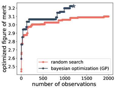
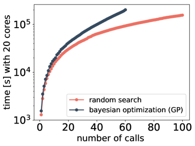
In both cases, to make a comparison using the same computing resources, the exploration of the parameter space at each call has been distributed among (=20) physical cores each evaluating a different point of the design space.111111It should be obvious that the duration of each call for a random search is independent of the number of simulations running in parallel on different cores. As the well known main drawback of the BO is that it scales cubically with the number of explorations, which is mainly due to the regression of the objective function through GPs (in Sec. 4, we discuss an improved strategy). Despite this, it typically converges to the optimum in a smaller number of iterations (and as the number of observations increase, it remains in the basin of attraction). A list of hyperparameters used in this framework can be found in Table 2.
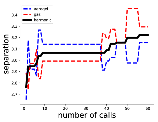
Table 3 summarizes the results of the optimization procedure based on the figure of merit in Eq. (3.2). Figure 6 shows the trade-off between the two regions in terms of PID performance found during the optimization process, where initially both aerogel and gas increase in separation power, and eventually after a certain number of calls a gain in the performance of the gas corresponds to a loss in the performance of the aerogel part. Another interesting feature is suggested by the results of Fig. 4: we can increase the refractive index of the aerogel only if we increase its thickness and maintain a sufficiently high enough yield of Cherenkov photons.121212The objective function (Eq. 3.1) at a given momentum is a trade-off between larger angular separation of two particle species (corresponding to lower refractive index) and larger number of photons (larger index of refraction and longer radiator). The number of produced photons will reach a plateau at some thickness value, due to the optical absorption length of the radiator material. It is also relevant the fact that some of the geometrically constrained parameters, as well as the aerogel related ones, reached their range boundaries; the dRICH development shall take into account these results.
| symbol | description | value |
|---|---|---|
| T | maximum number of calls | 100 |
| M | design points generated in parallel | 20 |
| N | pions (and kaons) per sample | 200 |
| kappa | controls variance in predicted values | 1.96 |
| xi | controls improvement over previous best values | 0.01 |
| noise | expected noise (relative) | 2.5% |
| FoM (h) | @ 14 GeV/c | @ 60 GeV/c | |
|---|---|---|---|
| BO | 3.23 | 3.16 | 3.30 |
| legacy | 2.9 | 3.0 | 2.8 |
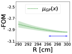
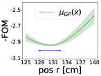
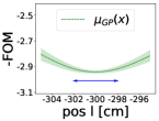
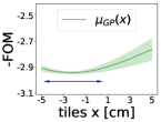
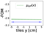
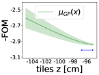
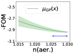
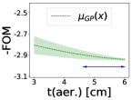
Since BO provides a model of how the FoM depends on the parameters, it is possible to use the posterior to define a tolerance on the parameters. Domain knowledge is required to decide how large of a change in the FoM is irrelevant, then the FoM space can be scanned to define how much each parameter can vary before seeing a relevant change. To this end, we use the proxy , where and are the expected value and standard deviation on the FoM as a function of provided by the model, and, in particular, is the optimal value found by the BO for the considered parameter. The tolerance interval is defined as the region where , this condition meaning a variation which is not statistically significant. The tolerance region of each parameter is drawn in Fig. 7 as a two-headed blue arrow on top of the corresponding marginalized posterior distribution obtained with BO. The values reported in Table 4 are obtained following the above strategy.
| parameter | results | tolerance region |
|---|---|---|
| R | 300.0 | (296.2,300.0) [cm] |
| pos r | 130.5 | (127.8,132.7) [cm] |
| pos l | -299.8 | (-302.0,-298.0) [cm] |
| tiles x | -2.8 | (-4.7,0.4) [cm] |
| tiles y | 5.0 | (-5.0,5.0) [cm] |
| tiles z | -95.00 | (-96.85,-95.00) [cm] |
| naerogel | 1.030 | (1.025, 1.030) |
| taerogel | 6.0 | (4.6, 6.0) [cm] |
The results discussed in the previous sections for the dRICH are very promising: Fig. 8 summarizes the overall improvement in PID performance over a wide range of momentum obtained with the Bayesian optimization compared to the baseline curve based on [6].
At least 3 separation is achieved in the aerogel region for GeV/c (compared to the baseline 12.5 GeV/c), whereas in the gas region the same separation is obtained for GeV/c (compared to 58 GeV/c).
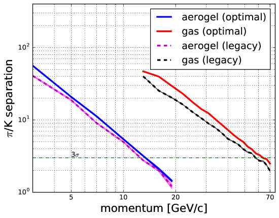
Both the baseline and the optimized curves have been calculated using charged tracks in the angular region (5,15) deg. As expected, once the optical properties of the aerogel are fixed (i.e. the refractive index dispersion curve, strictly connected with the single photon chromatic error), there is less room for a purely geometrical optimization of the system compared to the gas where the emission error is the dominant one and it is instead purely geometric.
4 Conclusions and Future Directions
We present for the first time an implementation of BO to improve the design of future EIC detectors, and we provide a detailed procedure to do this in a highly parallelized and automated way. We show in this case study that the PID capabilities of the current modeled dRICH detector can be substantially improved using our approach. In addition, the BO offers interesting hints on the relevance and correlation of the different parameters and it is possible to estimate the expected tolerances, within which any variation of the parameters does not alter the detector performance. We expect that the proposed BO method can provide improvements and hints for the future R&D of the dRICH, when results from prototype tests will validate and consolidate the current simulated model. More generally, real-world costs of the components could be included in the optimization process, either by extending the FoM or by exploring a Pareto optimization with multiple objective functions [33].
Currently, there are many ongoing efforts to simulate and analyse EIC detector designs, and the approach developed here—being completely general—can be employed for any such study. There are a variety of ways in which this study could be improved, which will be investigated in the near future. For example, in Appendix C, we introduce criteria for determining when to stop the optimization procedure, to avoid wasting resources if a suitable optimum has already been found. This work does not take into account the possible interplay between the dRICH and the other detectors. There is work ongoing on designing the TOF detector at very good timing resolution, and this will have an impact on the PID performance at low momentum. Therefore, a multi-detector design optimization is a possible future direction of this work. Another important aspect involves the choice of optimizing all the parameters together versus in blocks. For example, in the Pythia BO tune [27], better precision was obtained by optimizing the parameters in 3 blocks rather than all of them together. This worked because many observables were unaffected by several Pythia parameters. Once multi-detector optimizations are considered, it may be prudent to adopt a similar approach here. In addition, one can certainly test different figures of merit; however, the figure of merit defined in Eq. (3.2) is well suited to optimizing the dRICH design, see Appendix A. Novel Python frameworks for Bayesian optimizations like GPflowOpt [34] could improve the timing performance. This package is based on the popular GPflow library for Gaussian processes, leveraging the benefits of TensorFlow [35] including parallelization. Recently, optimization packages have been developed to rely on accelerated CUDA/GPU implementations. For example, Deep Networks for Global Optimization (DNGO) [36], where neural networks (NNs) are used as an alternative to GPs resulting in an improved scalability from cubic to linear as a function of the number of observations needed to explore the objective-function. The choice of hyperparameters of the NN is not defined a priori and in principle this could also be optimized with BO techniques to maximize the validation accuracy and inference time.
In conclusion, AI-based tools have been introduced and tested for the optimization of the dRICH configuration; the preliminary results clearly show a substantial improvement in performance and may provide useful hints on the relevance of different features of the detector. These same tools can be extended and applied to other detectors and possibly to the entire experiment, making the EIC R&D one of the first programs to systematically exploit AI in the detector-design phase.
Acknowledgments
We thank R. Yoshida for encouraging this work. This material is based upon work supported by the U.S. Department of Energy, Office of Science, Office of Nuclear Physics under contracts DE-AC05-06OR23177, DE-FG02-94ER40818. For this work, CF was supported by the EIC fellowship award at Jefferson Lab.
Appendix A Angular dispersion in RICH detectors
The error on the Cherenkov angle is given by several contributions, ; the error on the measured Cherenkov angle of a single photon is given by the quadratic sum of all the relevant contributions:
| (A.1) |
The single terms in the sum that we consider are the typical relevant contributions taken into account for similar dual-radiator RICHes in spherical reflecting mirror configuration (see [37, 38] for a compendium). The reconstruction of the Cherenkov angle in Fig. 3 is based on the GEMC simulation and the indirect ray tracing algorithm used by the HERMES experiment (see [10] for details on the algorithm). The following contributions are taken into account in the simulation.
Chromatic error:
The most important aspect in the choice of a Cherenkov radiator for a RICH detector is the index of refraction of the material and its characteristic optical dispersion. Namely, one of the terms in A.1 is due to the variation of the refractive index of the materials traveled by the photon of a given energy (or wavelenght ). In the case of a dual-radiator (let us assume aerogel and gas) this error consists of two contributions for the first radiator: the uncertainty on the photon emission wavelength depending on the dispersion relation () and the uncertainty on the refraction between aerogel and gas surface (). Therefore we have:
| (A.2) |
where
| (A.3) |
with the refractive index of the considered radiator. //For the emission contribution to the chromatic error, we have
| (A.4) |
and
| (A.5) |
The above can be also found in [37] using instead of . Notice that the variation of the refractive index of the aerogel, namely , can be inferred by recent measurements on the latest generation aerogel (i.e. the one tested by the CLAS12 RICH collaboration [15]). The uncertainty due to the refraction of the photons between the two materials, , is in general one order of magnitude lower than the chromatic aberration; nevertheless it has to be considered and somehow corrected in any kind of geometric reconstruction algorithm. For the second radiator (the gas in this case) only the first contribution is present. The chromatic error curves have been obtained using the following optical parameters:
-
•
aerogel and transmittance: the detailed study of the CLAS12 RICH collaboration has been used to infer the optical properties of recently manufactured aerogel [15]. Also the scattering length, and the related Rayleigh scattering have been introduced in the GEMC simulation. The photons with wavelength below 300 nm have been filtered simulating a thin acrylic slab placed between aerogel and the gas tank, for both shielding and avoiding aerogel chemical degradation;
-
•
properties from [39];
-
•
the mirror reflectance has been assumed the same of CLAS12 HTCC RICH mirrors (this is the GEMC mirror reference [16], the reflectance varies in the range of wavelength between 190 and 650 nm, consistent with the photon sensor quantum efficiency);
-
•
the quantum efficiency curve of the multi-anode PMT Hamamatsu-H12700-03 [18].
Emission error:
The focal plane shape has been chosen to be spherically-tessellated (about 4500 cm2 per sector, cm2 each tile). Due to the spherical aberrations the real focal plane for a spherical mirror is no longer a naive sphere. Therefore, the real shape of the focal surface will depend, point by point, on the angle (with respect to the optical axis) of incidence of the photon track on the mirror. Namely, this angle is known only statistically due to the fact that the emission point of each photon in the radiators is unknown.
Pixel-size error:
This corresponds to the uncertainty due to the granularity of the pixel detector, namely 3 mm pixel size in dRICH case.
Magnetic field error:
The dRICH is immersed in a non negligible magnetic field and the charged hadron tracks are bending as they pass through the Cherenkov radiators (and expecially the much longer gas). This introduces an additional source of error in the Cherenkov angle. The effect is proportional to the path length within the Cherenkov radiators, and therefore it becomes particularly important for the gas radiator at large polar angle.
Track error:
An angular track smearing of 0.5 mrad (1 mm over 2 m) has been assumed with very safe margin of technical feasibility.
Appendix B Noise Studies
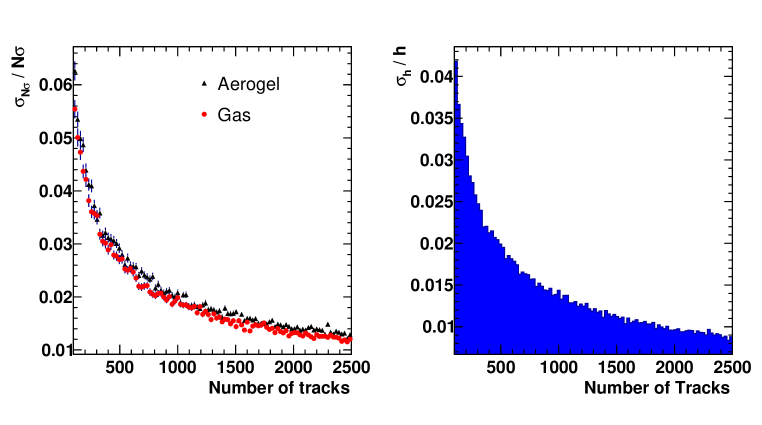
We investigated and characterized the statistical noise present on the objective function during the optimization process. Notice that Bayesian optimization takes into account this noise as an external parameter, e.g. skopt [30] allows to deal with this noise in different ways, for example by adding it (assumed to be ideal gaussian) to the Matérn kernel [28]. From simulations we have been able to determine the relative uncertainty on the figure of merit, which as expected scales (e.g. 2% if ).
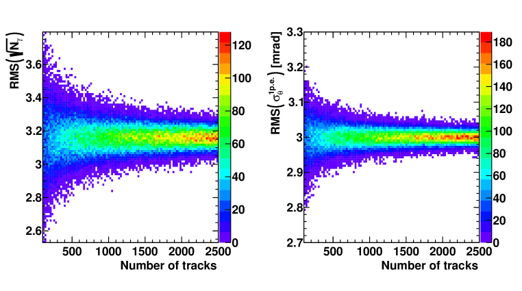
The relative fluctuations of the terms and (Fig. 9) contribute roughly equally in Eq. (3.2) as one can expect from the statistical errors propagation; these fluctuations are largely independent on the absolute values of the above terms (as demonstrated by the left plot in Fig. 10) and therefore on the charged particle momenta (as long as they are above Cherenkov threshold).
In the results shown in Fig. 9 and 10, we neglected the uncertainty on the difference between the mean angles, which is smaller than the uncertainty on and .
Appendix C Early stopping criteria
Each call is characterized by design points (generated in parallel), each being a vector in the parameters space defined in Tab. 1, with -dimensions. At each call , we can calculate the average point (vector) from the vectors (where ), as:
| (C.1) |
For a large number of calls (after a burn-in period chosen to be equal to 10 calls), the design point expressed by Eq. (C.1) tends to a global optimum steered by the BO.
In the following we will use the notation to express the element of the point, where and . At each call, we can also define the sample variance on each component of Eq. (C.1), in the following way:
| (C.2) |
Pre-processing of data consists in masking for each component the outliers distant by more than 3 from the average component. They correspond to very large explorations in the optimization process. Therefore, the effective number of points for each component and at each call becomes . and we can redefine the masked average and variance expressed in Eq. (C.1) (C.2) after removing these outliers. To simplify the notation, we will dub the masked mean and variance on every component as and .131313Standard deviations smaller than tolerances are replaced with the latter in Eqs. (C.3),(C.5).
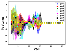
This allows to define the standardized variable:
| (C.3) |
Notice that Eq. (C.3) is defined comparing the values in the previous () and current () calls.141414Rigorously if 40 typically one refers to small sampling theory and a t-distibution should be considered. The stopping criteria have been implemented in a flexible way that allows to use either a standardized Z or t-distribution depending on the number of physical cores available. Now at each call and for each component, we can test the null hypothesis that and belong to a population with same mean , that is they are converging in the component to the same value. We do two-tailed p-value tests at 0.3% significance level (corresponding approximately to 3) for each component () in the parameter space.
| (C.4) |
The -functions in Eq. (C.4) represent boolean operators, that is each is 1 when the null is confirmed on the component. In addition, it is possible to build a Fisher statistic,
| (C.5) |
which can be used to determine whether or not the variance is significantly larger than at a certain significance level, e.g., 1%. This is done for all the components, similarly to what already discussed for (C.3), and enters as a multiplicative condition in (C.4). If all of them are 1 then the overall function becomes 1 too (in that case meaning the x stopper is activated). The stopping criteria on at the call corresponds to p-value tests all confirming the hypothesis as well. In order to stop the BO, the other condition (y stopper is activated) has to be satisfied along with Eq. (C.4).
| (C.6) |
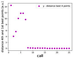
As for the value of the figure of merit , we consider at each call the best optimal values (e.g. ) obtained up to that call, and calculate the difference between the worst (largest) and the best (smallest) as151515In a minimization problem the lowest of the minima is considered the best value.
| (C.7) |
The statistic Eq. (C.7) vary typically rather smoothly if q5, and we can apply a cut on the relative variation between two successive calls, requiring
| (C.8) |
where is the arithmetic mean between and . The threshold values used to activate the above booleans have been chosen based on a toy model with the same number of parameters to tune. In conclusion, when the two conditions (C.4) and (C.8) are both activated or the maximum number of calls reached then the search is stopped. It should be clear that the empirical stopping criteria expressed in Eq. (C.4) and (C.8) are not sufficient to exclude the presence of a local optimum. Nevertheless Bayesian optimization is one of the most suitable tools to find a global optimum in a bounded region and we made dedicated studies in Appendix B to check the consistency of the values of our cuts when the stoppers are triggered with the expectations (e.g.,we know that the relative statistical uncertainty on the harmonic mean for a number of tracks equal to 400 is about 2%). We can also compare the results obtained using a regressor other than GP (e.g. GBRT, extra trees (ET), random forest (RF) regressors etc. [30]), as explained in the text. A simple random search is fast enough to run and can provide useful hints if the candidate point is far from the optimum.
Notice that (C.3) could produce potential issues if the RMS in the denominator is large compared to numerator. The following combined requirements prevent from these issues: (a) minimum number of burn-in calls, (b) all the booleans are true in Eqs. (C.6) and (C.8), (c) additional request that the above conditions (a) and (c) are true for a call and check that this holds in the successive call before activate the early stopping.
Another parameter to define is the maximum number of calls that stops the search in case the other stopping criteria did not trigger. We consider the heuristic formula determined by [27] as a possible lower bound.161616An hand-waving estimate for the number of calls needed when running simulations in parallel is obtained by scaling that number by . Clearly the total number of calls can be set to any larger value provided enough computing/time resources.
References
- [1] D. R. Jones, M. Schonlau, W. J. Welch, Efficient global optimization of expensive black-box functions, J. Global Optim. 13 (4) (1998) 455–492. doi:10.1023/A:1008306431147.
- [2] J. Snoek, H. Larochelle, R. P. Adams, Practical bayesian optimization of machine learning algorithms, in: Adv. Neural Inf. Process. Syst., (2012), pp. 2951–2959. arXiv:1206.2944.
- [3] A. Accardi, et al., Electron-Ion Collider: The next QCD frontier, Eur. Phys. J. A 52 (9) (2016) 268. arXiv:1212.1701, doi:10.1140/epja/i2016-16268-9.
- [4] National Academies of Sciences, Engineering, and Medicine, An Assessment of U.S.-Based Electron-Ion Collider Science. (2018). doi:10.17226/25171.
- [5] E. Aschenauer, et al., Electron-Ion Collider Detector Requirements and R&D Handbook (Version 1.1) (2019).
- [6] A. Del Dotto, et al., Design and R&D of RICH detectors for EIC experiments, Nucl. Instrum. Meth. A 876 (2017) 237–240. doi:10.1016/j.nima.2017.03.032.
- [7] C. Wong, et al., Modular focusing ring imaging Cherenkov detector for electron-ion collider experiments, Nucl. Instrum. Meth. A 871 (2017) 13–19. doi:10.1016/j.nima.2017.07.001.
- [8] G. Kalicy et al., High-performance DIRC detector for the future Electron Ion Collider experiment, J. Instrum. 13 (4) (2018) C04018. doi:10.1088/1748-0221/13/04/C04018.
- [9] D. Romanov, JLEIC Detector and Simulation (Jefferson Lab 2019 Users Organization), www.jlab.org/user_resources/meetings/JLUO_6_19/Romanov.pptx (2019).
- [10] N. Akopov, et al., The HERMES Dual-Radiator Ring Imaging Cherenkov Detector, Nucl. Instrum. Meth. A 479 (2) (2002) 511–530. arXiv:0104033, doi:10.1016/S0168-9002(01)00932-9.
- [11] The LHCb Collaboration, A. Alves Jr, et al., The LHCb Detector at the LHC, J. Instrum. 3 (2008) S08005. doi:10.1088/1748-0221/3/08/S08005.
- [12] The LHCb Collaboration, M. Adinolfi, et al., Performance of the LHCb RICH detector at the LHC, Eur. Phys. J. C 73 (5) (2013) 1–17. doi:10.1140/epjc/s10052-013-2431-9.
- [13] The LHCb Collaboration, A. Alves Jr, et al., The LHCb detector at the LHC, J. Instrum. 3 (08) (2008) S08005. doi:10.1088/1748-0221/3/08/S08005.
- [14] The LHCb Collaboration, R. A. Nobrega, et al., LHCb reoptimized detector design and performance: Technical Design Report, Tech. Rep. No. CERN-LHCC-2003-030; LHCb-TDR-9 (2003).
- [15] S. Pereira, et al., Test of the CLAS12 RICH large-scale prototype in the direct proximity focusing configuration, Eur. Phys. J. A 52 (2) (2016) 1–15. arXiv:1509.02818, doi:10.1140/epja/i2016-16023-4.
-
[16]
M. Ungaro, et al., Geant4 Monte Carlo (GEMC).
URL http://gemc.jlab.org - [17] M. Contalbrigo, et al., Aerogel mass production for the CLAS12 RICH: Novel characterization methods and optical performance, Nuc. Instrum. Meth. A 876 (2017) 168–172. doi:https://doi.org/10.1016/j.nima.2017.02.068.
- [18] Hamamatsu, Datasheet: Flat Panel Type Multianode PMT Assembly H12700 SERIES / H14220 SERIES, https://www.hamamatsu.com/resources/pdf/etd/H12700_H14220_TPMH1379E.pdf.
- [19] 16th Electron Ion Detector R&D Meeting, https://wiki.bnl.gov/conferences/index.php/Reports-January2019 (2019).
- [20] E. Brochu, V. M. Cora, N. De Freitas, A Tutorial on Bayesian Optimization of Expensive Cost Functions, with Application to Active User Modeling and Hierarchical Reinforcement Learning (2010). arXiv:1012.2599v1.
-
[21]
B. Eric, N. D. Freitas, A. Ghosh,
Active
preference learning with discrete choice data, in: J. C. Platt, D. Koller,
Y. Singer, S. T. Roweis (Eds.), Adv. Neural Inf. Process Syst., Curran
Associates, Inc., (2008), pp. 409–416.
URL http://papers.nips.cc/paper/3219-active-preference-learning-with-discrete-choice-data.pdf -
[22]
E. Brochu, T. Brochu, N. de Freitas,
A Bayesian
Interactive Optimization Approach to Procedural Animation Design, in:
Proceedings of the 2010 ACM SIGGRAPH/Eurographics Symposium on Computer
Animation, SCA ’10, Eurographics Association, Goslar Germany, Germany,
(2010), pp. 103–112.
URL http://dl.acm.org/citation.cfm?id=1921427.1921443 - [23] D. J. Lizotte, T. Wang, M. H. Bowling, D. Schuurmans, Automatic Gait Optimization with Gaussian Process Regression., in: IJCAI, Vol. 7, (2007), pp. 944–949.
- [24] N. Srinivas, A. Krause, S. M. Kakade, M. W. Seeger, Information-theoretic regret bounds for gaussian process optimization in the bandit setting, IEEE T. Inform. Theory 58 (5) (2012) 3250–3265. doi:10.1109/TIT.2011.2182033.
- [25] F. Hutter, H. H. Hoos, K. Leyton-Brown, Sequential model-based optimization for general algorithm configuration, in: International Conference on Learning and Intelligent Optimization, Springer, (2011), pp. 507–523. doi:10.1007/978-3-642-25566-3_40.
-
[26]
J. Bergstra, D. Yamins, D. D. Cox,
Hyperopt:
A python library for optimizing the hyperparameters of machine learning
algorithms, in: Proceedings of the 12th Python in science conference,
Citeseer, (2013), pp. 13–20.
URL http://citeseerx.ist.psu.edu/viewdoc/summary?doi=10.1.1.704.3494 - [27] P. Ilten, M. Williams, Y. Yang, Event generator tuning using Bayesian optimization, Journ. of Instrum. 12 (04) (2017) P04028. arXiv:1610.08328, doi:10.1088/1748-0221/12/04/P04028.
- [28] C. K. Williams, C. E. Rasmussen, Gaussian processes for machine learning, Vol. 2, MIT press Cambridge, MA, (2006). doi:10.1007/978-3-540-28650-9_4.
- [29] R. Bellman, Dynamic Programming, Rand Corporation research study, Princeton University Press, (1957). doi:10.1073/pnas.38.8.716.
- [30] T. Head, et al., scikit-optimize/scikit-optimize: v0.5.2 (Version v0.5.2), Zenodo. http://doi.org/10.5281/zenodo.1207017, march 25 (2018).
- [31] J. H. Friedman, Greedy function approximation: a gradient boosting machine, Annals of statistics (2001) 1189–1232.
-
[32]
J. Bergstra, Y. Bengio,
Random
search for hyper-parameter optimization, J. Mach. Learn. Res. 13 (Feb)
(2012) 281–305.
URL http://jmlr.csail.mit.edu/papers/volume13/bergstra12a/bergstra12a.pdf - [33] P. Ngatchou, A. Zarei, A. El-Sharkawi, Pareto multi objective optimization, in: Proceedings of the 13th International Conference on, Intelligent Systems Application to Power Systems, IEEE, (2005), pp. 84–91. doi:10.1109/ISAP.2005.1599245.
- [34] N. Knudde, J. van der Herten, T. Dhaene, I. Couckuyt, GPflowopt: A Bayesian optimization library using tensorflow, (2017). arXiv:1711.03845.
- [35] M. Abadi, et al., Tensorflow: Large-scale machine learning on heterogeneous distributed systems, (2016). arXiv:1603.04467.
- [36] J. Snoek, et al., Scalable bayesian optimization using deep neural networks, in: International conference on machine learning, (2015), pp. 2171–2180. arXiv:1502.05700.
- [37] E. Nappi, J. Seguinot, Ring Imaging Cherenkov Detectors: The state of the art and perspectives, Riv. Nuovo Cimento 28 (8-9) (2005) 1–130. doi:10.1393/ncr/i2006-10004-6.
- [38] T. Ypsilantis, J. Séguinot, Theory of ring imaging Cherenkov counters, Nuclear Instruments and Methods in Physics Research Section A: Accelerators, Spectrometers, Detectors and Associated Equipment 343 (1) (1994) 30–51. doi:10.1016/0168-9002(94)90532-0.
- [39] R. Abjean, A. Bideau-Mehu, Y. Guern, Refractive index of hexafluoroethane (C2F6) in the 300-150 nm wavelength range, Nucl. Instrum. Methods Phys. Res. A 354 (2-3) (1995) 417–418. doi:10.1016/0168-9002(94)01006-4.