A scalable weakly-synchronous algorithm for solving partial differential equations

Abstract

Synchronization overheads pose a major challenge as applications advance towards extreme scales. In current large-scale algorithms, synchronization as well as data communication delay the parallel computations at each time step in a time-dependent partial differential equation (PDE) solver. This creates a new scaling wall when moving towards exascale. We present a weakly-synchronous algorithm based on novel asynchrony-tolerant (AT) finite-difference schemes that relax synchronization at a mathematical level. We utilize remote memory access programming schemes that have been shown to provide significant speedup on modern supercomputers, to efficiently implement communications suitable for AT schemes, and compare to two-sided communications that are state-of-practice. We present results from simulations of Burgers’ equation as a model of multi-scale strongly non-linear dynamical systems. Our algorithm demonstrate excellent scalability of the new AT schemes for large-scale computing, with a speedup of up to $3.3$x in communication time and $2.19$x in total runtime. We expect that such schemes can form the basis for exascale PDE algorithms.

1 Introduction

Numerical simulations are an important tool in the pursuit of understanding critical problems in science and engineering. Many natural phenomena and engineered systems are described using highly non-linear partial differential equations (PDEs). At the conditions of practical interest, non-linearity in the equations results in a multi-scale phenomena which demands massive computations at extreme levels of parallelism. Current state-of-the-art simulations are routinely being carried out on hundreds of thousands of processing elements (PEs) [1, 2, 3, 4]. It has been observed at large scale that data synchronizations between PEs and communications result in poor scalability of applications. On future exascale machines, which will consist of millions of PEs, the scalability of applications is expected to be further compromised. There are several efforts at various levels of the stack (hardware, software and algorithms) to relax the data synchronization and avoid communication [5, 6, 7].

In time-dependent PDE solvers, the governing equations are approximated with spatial and temporal schemes which result in algebraic equations. These equations are solved at each grid point in a discrete computational domain (e.g., see Figure 1 (a)), for given initial and boundary conditions, to obtain the solution of a function at a time instant or level. This process is repeated in a time-marching or iterative manner to arrive at a time evolved solution. Typically, computations at a generic point $i$ depend on the value of the function at its neighbors. The extent of the neighborhood is determined by the spatial schemes, which is referred to as a stencil. To parallelize the computations in a solver, the set of grid points in a domain is decomposed into $P$ subsets that are then distributed to $P$ compute processes, as illustrated in Figure 1 (b). If not all the stencil points for a grid point $i$ are in the same subset (i.e., $i$ is a process boundary point), then the function values of the missing points have to be communicated to the owner process of point $i$, before the computations are advanced. This communication is often facilitated through the so called buffer or halo points, which can be understood as a local cache of the remote values. These buffers can also be seen as the special case of a one-time producer-consumer queue: at each iteration producers communicate new values into the buffer and consumers wait until the data becomes available. We call PDE algorithms that rely on synchronized buffer data to advance computations from a time level $n$ to $n+1$ as synchronous algorithms.

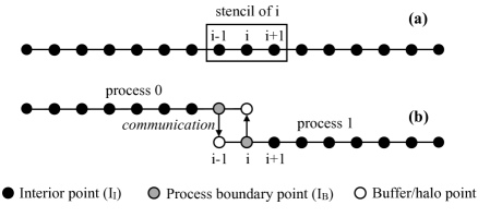
Figure 1: Schematic of discretized one-dimensional domain decomposed into two processes ($P=2$).

In simple synchronous algorithms, both receivers have to wait for senders and senders may have to wait for receivers. The latter synchronization can be relaxed either implicitly with message buffering [8], which is feasible only for small messages, or explicitly with multi-version variables that expose the buffer as a producer-consumer queue with multiple entries [9]. Yet, the receiver still has to wait for the sender to guarantee consistent data in the buffer. Due to the iterative nature of PDE computations, this synchronization prevents two processes from running more than one iteration apart in real-time—a very stringent requirement for large-scale systems where delays are normal and propagate quickly [10].

With increasing degree of parallelism, the size of the point set per process shrinks and, relatively more stencil points are at remote processes. Thus, the communication and synchronization overhead grows steadily while the iteration compute time per process shrinks. On future exascale systems, it can be expected that the communication time is equivalent or higher than the computation time, thus, the smallest process delays will lead to high synchronization overheads. In addition, future large-scale systems are expected to exhibit a higher performance variability than today’s systems [11], further aggravating the overheads due to process synchronization.

This work presents a method to relax the synchronization further such that the receiver does not wait for the sender and computations at process boundary points are performed with potentially outdated values. The concept and mathematical feasibility of such an asynchronous computational approach for PDEs has been studied [12, 13], and is summarized in Section 2. New asynchrony-tolerant (AT) finite-difference schemes [13] will be used to design a novel and accurate weakly-synchronous algorithm for PDE solvers, which can proceed with computations of $L$ time level advancements in an asynchronous fashion (data at halo points can be up to $L$ iterations apart). The performance of the algorithm will be compared with commonly used synchronous algorithm to demonstrate the scalability of weakly-synchronous (WS) algorithm at large scales. Two different communication models, one-sided remote memory access and two-sided message passing, are used to evaluate the effect of different parallel programming models.

The rest of the paper is organized as follows. The mathematical background of asynchronous computing for PDEs is described in Section 2. Simulation details of a benchmark problem are presented in Section 3. The parallel programming models to implement data communication are described in Section 4. section 5 illustrates the synchronous and weakly-synchronous algorithms and their implementation. Results on numerical accuracy and computational performance are reported in Section 6. Related work and conclusions are discussed in sections 7 and 8, respectively.

2 Mathematical Background

In a PDE solver, the basic requirement of data synchronization between PEs is imposed by the numerical method, and in particular, computation of the spatial derivatives. When this is relaxed at a mathematical level, other synchronizations in the computing algorithm can also be relaxed. To understand this in a mathematical perspective, consider the computations at the grid point $i$ in Figure 1 (b), which assumes a three point stencil. Let $f$ be a function whose solution is advanced from a time level $n$ to $n+1$ in an iteration. As the owner process of $i-1$ is different from $i$, the value of $f$ at $i-1$ is communicated into the halo point at each iteration. We refer to these communications as halo exchanges. In synchronous algorithms, computations at $i$ cannot proceed unless $f$ at the buffer point $i-1$ is at time level $n$. As mentioned earlier, this is ensured by explicit synchronization. The spatial derivatives in synchronous algorithms are computed with uniform time level of the function at all the points in a stencil. For explicit-in-time schemes, the function will be at the time level $n$. We refer to such computations as synchronous computations.

In the asynchronous computing approach [14, 12], values of $f$ are communicated in halo exchanges at each time iteration, however the synchronization is not imposed. This means that the value of $f$ in the halo points may not be at time level $n$. Depending on the speed of communication, the time level can be from one of the $n$, $n-1$, $n-2$, $\dots$ levels. Let $\tilde{n}=n-{\tilde{k}}$ denote the latest time level of $f$ available at a halo point, where ${\tilde{k}}$ indicates the delay in terms of number of levels. If $\tilde{n}=n$ or ${\tilde{k}}=0$, then the time level of $f$ at a halo point is synchronous. Otherwise, if $\tilde{n}<n$ or ${\tilde{k}}>0$, then $f$ is at an asynchronous or delayed time level. As the delay cannot be indefinite, we restrict the maximum allowable delay to $L$ time levels, which means $\tilde{n}\in\{n,n-1,\dots,n-L+1\}$. If the delay at a halo point exceeds $L$, then a synchronization of messages has to be imposed to reduce the delay value to be less than $L$. For this reason, we refer to the algorithm for the asynchronous computing approach as a weakly-synchronous algorithm.

Considering a non-zero probability of having an asynchronous value of $f$ at halo points, let us examine the nature of computations carried out at grid points in the domain. For interior points (see Figure 1 (b)), all the points in their stencil are computed in the same process, and the function values will be at a time level $n$. Hence, computations at these points are synchronous. On the other hand, some of the points in the stencil of a process boundary point are halo points, and the time level $\tilde{n}$ of $f$ at the halo points can be synchronous or asynchronous. The computations at process boundary points are synchronous if $\tilde{n}=n$ (i.e., $f$ is synchronous). Otherwise, the time level of $f$ at different points in the stencil is non-uniform and we refer to these computations at process boundary points as asynchronous computations. Clearly, the nature of computations at process boundary points depends on how fast the messages are delivered.

An analysis based on the finite-difference method [12] showed that numerical properties of standard schemes, when computations are performed in an asynchronous fashion, will not only depend on numerical parameters like the grid resolution ($\Delta x$) and time step ($\Delta t$), but also on simulation parameters like the number of processes ($P$) used in a simulation and the characteristics of communication or the delay (${\tilde{k}}$). It has also been demonstrated that while standard schemes are able to maintain stability as well as consistency, their accuracy is significantly affected. The reduced accuracy is attributed to terms in the truncation error of schemes that appear due to asynchrony. In a subsequent study [13], new asynchrony-tolerant (AT) schemes with arbitrary order of accuracy have been derived. These schemes use a wider stencil to eliminate the low order asynchrony terms in the truncation error and result in a higher order accuracy. The wider stencil of AT schemes, relative to standard schemes, can be obtained either by adding more points in space or by using multiple time levels of the function at each stencil point. The former leads to larger message sizes and the latter increases the memory requirements of a process. The AT schemes used in this paper are shown below. The expressions for the schemes evaluated at a grid point $i$ and time level $n$ are, for a delay on the left side of the stencil,

$$\left.\dfrac{\partial{f}}{\partial{x}}\right|_{i}^{n} = \frac{f_{i+1}^{n}-({\tilde{k}}+1)f_{i-1}^{n-{\tilde{k}}}+{\tilde{k}}f_{i-1}^{n-{\tilde{k}}-1}}{2\Delta x}+\mathcal{O}\left(\Delta x^{2}\right)$$

$$\left.\frac{\partial^{2}f}{\partial x^{2}}\right|_{i}^{n} = \frac{f_{i+1}^{n}-2f_{i}^{n}+({\tilde{k}}+1)f_{i-1}^{n-{\tilde{k}}}-{\tilde{k}}f_{i-1}^{n-{\tilde{k}}-1}}{\Delta x^{2}}$$ (1)

$$+\mathcal{O}\left({{\tilde{k}}({\tilde{k}}+1)}{\Delta t^{2}}/{\Delta x^{2}},\Delta x^{2}\right).$$

And, for a delay on the right side of the stencil,

$$\left.\dfrac{\partial{f}}{\partial{x}}\right|_{i}^{n} = \frac{({\tilde{k}}+1)f_{i+1}^{n-{\tilde{k}}}-{\tilde{k}}f_{i+1}^{n-{\tilde{k}}-1}-f_{i-1}^{n}}{2\Delta x}+\mathcal{O}\left(\Delta x^{2}\right)$$

$$\left.\frac{\partial^{2}f}{\partial x^{2}}\right|_{i}^{n} = \frac{({\tilde{k}}+1)f_{i+1}^{n-{\tilde{k}}}-{\tilde{k}}f_{i+1}^{n-{\tilde{k}}-1}-2f_{i}^{n}+f_{i-1}^{n}}{\Delta x^{2}}$$ (2)

$$+\mathcal{O}\left({{\tilde{k}}({\tilde{k}}+1)}{\Delta t^{2}}/{\Delta x^{2}},\Delta x^{2}\right).$$

Here, the second term on the right hand side of each expression represents the truncation error with leading order terms shown in the parenthesis. These schemes are second order accurate in space when the time step in the simulations varies as $\Delta t\sim\Delta x^{2}$. It can be shown [13] that, to leading order, the average error ($\langle E\rangle$) due to asynchronous computations for these schemes is

$$\langle E\rangle\sim\frac{P}{N}\Delta x^{2}\left(\overline{{\tilde{k}}^{2}}+\overline{{\tilde{k}}}\right),$$ (3)

where, $N$ is the number of grid points in the domain, and $\overline{{\tilde{k}}^{2}}$ and $\overline{{\tilde{k}}}$ are moments of the delay ${\tilde{k}}$ measured during the course of the simulation. This equation shows that the error scales linearly with an increase in the number of processes, and goes up with an increase in the degree of asynchrony. However, these affects are diminished by the term $\Delta x^{2}$, which provides a control parameter to obtain solutions of desired accuracy.

3 Simulation Details

To demonstrate the implementation of the weakly-synchronous algorithm, we choose a problem of high relevance in practical applications. This section describes the problem definition and the governing PDEs, the numerical method, and the choice of programming model for communications between the processes.

3.1 Problem Definition

The viscous Burgers’ equation provides a rich model to understand the multi-scale phenomena in fluid flows. We simulate Burgers’ turbulence in a three-dimensional domain as a benchmark problem in this paper. In addition to the equations governing the velocity field, we also solve scalar advection-diffusion equations to replicate the computational complexities in many fluid flow solvers. Scalars are often used in simulations of turbulence to understand its mixing properties [2]. In reacting flow solvers [15], which are used to simulate combustion processes, scalars are transported representing different species in a chemical mechanism. The governing equations of the problem are

$$\frac{\partial u_{i}}{\partial t}+u_{j}\dfrac{\partial{u_{i}}}{\partial{x_{j}}} = \nu\frac{\partial^{2}u_{i}}{\partial x_{j}^{2}}\hskip 14.22636pt\text{ for $j=1,2,3$ and}$$

$$\frac{\partial\phi_{k}}{\partial t}+u_{j}\dfrac{\partial{\phi_{k}}}{\partial{x_{j}}} = \alpha_{k}\frac{\partial^{2}\phi_{k}}{\partial x_{j}^{2}},$$ (4)

where $u_{i}$ ($i=1,2,3$) represents the velocity component in the $i$th direction and $\nu$ is the kinematic viscosity of the fluid. $\phi_{k}$ and $\alpha_{k}$ are the concentration and diffusivity of the $k$th scalar, respectively. The equations are solved in a periodic domain with equal sides. Initial conditions are derived from a multi-scale sinusoidal function.

3.2 Numerical Method

Figure 2: Graph of average error convergence with increase in grid points. In the graph: (blue-circle line) configuration with synchronous algorithm and standard schemes, (red-triangle line) configuration with weakly-synchronous algorithm and standard schemes, (green-square line) configuration with weakly-synchronous algorithm which uses standard schemes for synchronous computations and AT schemes for weakly-synchronous computations, (black line) a reference line with slope equal to $-2$. Simulations are done with $P=8$.

The PDEs in Eq. 4 are solved using the finite difference method. To aid the description of numerical schemes for synchronous and weakly-synchronous algorithms, we define different subsets of grid points in a process. Let $I$ denote the set of points where the solution of $u_{i}$ and $\phi_{k}$ is computed. The set $I$ is further divided into ${I_{I}}$ and ${I_{B}}$. ${I_{I}}$ is the set of interior points whose computations do not depend on communication between processes. The points near process boundaries belong to set ${I_{B}}$, and their computations depend on communications.

Time integration is performed with the Euler scheme that is first order accurate in time and with a stability condition based on viscous/diffusive process ($\Delta t\sim\Delta x^{2}$), which results in second order accuracy in space. The spatial derivatives at a grid point $i\in{I_{I}}$ are computed using standard second order accurate central difference schemes. At process boundary points, i.e., $i\in{I_{B}}$, the stencil computations are asynchronous when there is a delay in communication. We use AT schemes in Eqs. (1) and (2) to compute the spatial derivatives. Note that for ${\tilde{k}}=0$, these AT schemes reduce to the standard central difference schemes used at interior points. This helps in homogenizing the error in the domain and lower the overall error in the solution [13].

Before proceeding to the next section, the affect of asynchrony on the accuracy of standard central difference schemes and the role of AT schemes used for computations in the set ${I_{B}}$ are demonstrated. Numerical simulations of a one-dimensional linear advection-diffusion equation are used for this purpose. The numerical schemes and initial and boundary conditions are the same as the one described above for the Burgers’ turbulence problem. The advection-diffusion equation has a simple analytical solution for this setup, which is used to compute the exact error in the computed solution and to provide a verification for the accuracy of algorithms. The simulations are performed in three different configurations. The first configuration computes with a synchronous algorithm using standard schemes. The second configuration computes with the weakly-synchronous algorithm using standard central difference schemes for points in sets ${I_{I}}$ and ${I_{B}}$. In the third configuration, the weakly-synchronous algorithm with standard schemes for points in ${I_{I}}$ and AT schemes for points in ${I_{B}}$ are used. Figure 2 shows how the error in the solution varies with an increase in the number of grid points. For the first configuration (blue-circle line), which uses the synchronous algorithm, the error decreases with a slope equal $-2$. This is expected since the schemes used are second order accurate. When the standard schemes are used in a weakly-synchronous algorithm (red-triangle line), due to the asynchronous computations at process boundaries the accuracy reduces drastically. However, this loss in accuracy of the weakly-synchronous algorithm is recovered by using AT schemes at ${I_{B}}$, as indicated by the green-square line in the figure which has a slope equal to $-2$. Aditya et al. [13] present a more detailed analysis for arbitrary order of accuracy.

4 Parallel Programming Models

The asynchronous computing approach imposes three requirements that parallel programming models should facilitate. First, they should enable communication without explicit synchronization at each time step. Second, they should store data from multiple time levels. And third, they should have knowledge of time level associated with each message. In terms of performance, the communication speed between process, which depends on the parallel programming model, not only effects the scalability, but also the numerical accuracy of the solution (e.g., as shown in Eq. 3). Hence, it is important to choose a fast, low-overhead parallel programming model that fulfills the above mentioned requirements in developing the weakly-synchronous algorithm.

4.1 Two-sided MPI

Two-sided MPI is the dominant parallel programming model in high-performance computing. To move data between the processes running on a distributed memory machine, the source and target processes call the MPI library to send and receive the data via the network. The popularity of two-sided MPI may be attributed to its performance and ease of use when developing bulk synchronous applications that alternate between computation and communication. However, every data transfer using two-sided MPI entails target interactions, such as the receive buffer address resolution, that prevent an efficient implementation of weak synchronization. The non-blocking interface suggests the possibility of overlapping communication and asynchronous computation. Yet, the limited hardware support necessitates periodic calls to the MPI library to guarantee asynchronous progress, which affects complexity and performance of a possible implementation [16]. We use the non-blocking interface to implement baseline variants of our communication algorithms.

4.2 Notified Remote Memory Access

One-sided MPI exploits the RDMA (Remote Memory Direct Access) capabilities of modern network interconnects to guarantee asynchronous progress. Using one-sided MPI, only the source process calls the MPI library and provides all information necessary to move the data directly to the target memory. This direct access enables hardware acceleration and avoids target interactions, such as the receive buffer address resolution. Moreover, the source and target processes are able to progress independently, which is key for an efficient implementation of weak synchronization.

Like most RMA (Remote Memory Access) implementations, one-sided MPI explicitly differentiates data movement and synchronization. This separation enhances the expressiveness and flexibility of the programming model at the cost of additional synchronization overheads. To avoid this performance penalty, the foMPI-NA [17] programming model introduces notified RMA. With foMPI-NA, the source process attaches a notification to the RMA. After completion of the data transfer, the network interconnect pushes the notification to a queue in the target memory. To synchronize, the target process queries the queue for incoming notifications. This mechanism enables efficient one-way synchronization using existing MPI design concepts. The MPI_Win_allocate method allocates memory segments called windows that provide hardware supported RMA. The processes call the method collectively and use the window to address the remote memory. The MPI_Put_notify method writes to remote memory and after completion notifies the target with the given tag. The method uses the window and displacement parameters to address the remote memory of the target process. The MPI_Win_flush_all method waits for the remote completion of pending accesses on the window. The MPI_Notify_init method implements notification matching based on persistent requests. The method parameters specify after how many notifications the matching completes. The matching filters notifications according to their tag and source process information. The MPI_Start method resets the persistent requests and starts the notification matching. The MPI_Test and MPI_Wait methods test and wait for the completion of the notification matching.

We implement the main variant of our communication algorithms with foMPI-NA since the programming model best fits the requirements of weak synchronization. The RMA semantics enables transferring data without target interaction and the notification queue enables querying the synchronization status without source interaction. As a result, the source and target processes can progress independently enabling maximum asynchrony.

5 Implementation

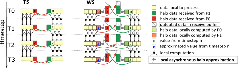
Figure 3: The TS algorithm synchronizes the processes after every time step, while the WS algorithm avoids synchronization if the process asynchrony stays within given bounds.

At scale, communication costs in PDE solvers are likely to dominate the overall runtime. This can be clearly observed in strong scaling a problem, which reduces the computational effort per process and significantly increases the number of communications. Also, the communication costs are often affected by system noise, which increase the costs further. Hence, recent advances in solver algorithms have a paradigm shift away from optimizing computations towards more efficient communication algorithms. These issues are addressed in the asynchronous computing approach, which naturally overlaps computations and communications, hiding the communication costs and reducing the impact of noise. In our weakly-synchronous algorithm, we exploit the benefits of the mathematical framework by designing an implementation with minimal compute and synchronization overheads.

We evaluate performance and scalability of the weakly-synchronous (WS) algorithm compared to the traditional synchronous (TS) algorithm. Figure 3 explains the halo exchange communication performed by the two algorithms that otherwise share the time loop which besides the communication implements the stencil computations to advance the solution to the next time step. The TS algorithm always exchanges the halo points of the current time step, which synchronizes the execution of the neighboring processes. The WS algorithm always sends the halo points of the current time step and immediately advances the solution using the latest available halo points. The algorithm employs circular buffers to store the halo points of multiple time levels and updates the boundary points using the AT schemes discussed in Section 3.2. This approach avoids synchronization at the cost of few additional computations at comparable numerical accuracy.

name	description
N	number of neighbors to communicate with
T	number of entries in the circular buffers
L	maximal allowable delay
sbuf/rbuf	send/receive buffers
sbnd/rbnd	bounds of the halo/boundary zones
roff	offset of the receive buffers in the target window
nbr	identifiers of the neighbor processes
rqst	notification matching requests
data	data array for local computations
$t_{s}$	send time step of the outgoing data
$t_{r}$	receive time step of the last incoming data
$t_{c}$	time step constraint (synchronize if $t_{c}>t_{r}$)
$h_{s}$	send head pointing to the buffer entry of $t_{s}$
$h_{r}$	receive head pointing to the buffer entry of $t_{r}$

Table 1: Main variables of our implementation

We implement the two algorithms with the one-sided foMPI-NA programming model (NA) discussed in Section 4.2 and for comparison provide variants based on the non-blocking interface of two-sided MPI (NB). We allocate one send-receive buffer pair per neighbor to communicate the data along all six faces of the cuboidal sub-domains. When running the WS algorithm, we allocate additional receive buffers that store the halo points of the last $L$ time levels and use tags to distinguish incoming notifications and messages from the different time levels. All notified access implementations place the send and receive buffers at different offsets within one window, move the data with notified RMA, and synchronize the execution using one notification per direction and time step. All two-sided implementations pre-post non-blocking receives for the next time levels, move the data using non-blocking sends, and wait for the completion of the receive requests to synchronize the execution. Pre-posting the receives is the only algorithmic difference when switching from one-sided to two-sided. The synchronous (TS-NB) algorithm pre-posts the receives for the next time level while the weakly-synchronous (TS-NB) algorithm pre-posts receives for maximal allowable delay L time levels. Apart from this difference, the two-sided variants are equal to the notified access based variants of the weakly-synchronous (WS-NA) and synchronous (TS-NA) algorithm next discussed in detail.

5.1 Traditional Synchronous Algorithm (TS-NA)

The TS algorithm exchanges the halo points of the current time level after every time step and synchronizes computation and communication. The algorithm overlaps the communications to the neighbor process but waits for their completion before proceeding with the next time step. Although this blocking design prevents any overlap of computation and communication, the TS algorithm is widely used in today’s PDE solvers. This ubiquity originates from the simplicity and maturity of the algorithm that enables high compute and communication throughput.

1

// send boundary points

2 for $i\leftarrow 1$ to N do

3       sbuf[:,$i$] $\leftarrow$ data[sbnd[$i$]];

4       MPI_Put_notify(sbuf[:,$i$],nbr[$i$],win,roff[$i$]);

5      

6 end for

7 MPI_Win_flush_all(win);

// receive halo points

8 for $i\leftarrow 1$ to N do

9       MPI_Start(rqst[$i$]);

10       MPI_Wait(rqst[$i$]);

11       data[rbnd[$i$]] $\leftarrow$ rbuf[:,$i$];

12      

13 end for

Algorithm 1 Synchronous halo exchange

Algorithm 1 shows the synchronous halo exchange (TS-NA). The algorithm supports a configurable number of neighbors N. The arrays sbuf and rbuf contain one send and receive buffer per neighbor. The arrays sbnd and rbnd store the index ranges that locate the boundary and halo points in the data array. The nbr array stores the process identifiers that in combination with the window provide access to the neighbor memories. The roff array stores the receive buffer offsets per neighbor. The offsets are relative with respect to the window. The rqst array stores one request per neighbor that matches one notification sent by the particular neighbor. We initialize the persistent requests at program startup and call the start method to reset them during the program execution.

On lines 1–1, we send the boundary points to all neighboring processes. We first pack the boundary points to the send buffer and then call the notified put method. We address the remote memory by combining process identifier, window, and receive buffer offset. After the send phase, we call the flush method to guarantee the completion of the sends.

On lines 1–1, we receive the halo points of all neighboring processes. We call the start and wait methods to match the incoming notifications. Once the data is available, we unpack the receive buffer to the halo points.

// communicate boundary

1 MPI_Win_flush_all(win);

$t_{s}\leftarrow t_{s}+1$;

  // update send time

$h_{s}\leftarrow\textnormal{{$t_{s}$}}\mod{\textnormal{{T}}}$;

  // map to circular buffer offset

2 for $i\leftarrow 1$ to N do

3       sbuf[:,$i$] $\leftarrow$ data[sbnd[$i$]];

4       $d\leftarrow\textnormal{{roff[}}\textnormal{\emph{$i$}}\textnormal{{]}}+h_{s}\times|\textnormal{{sbuf[}}\textnormal{\emph{:,i}}\textnormal{{]}}|$;

5       MPI_Put_notify(sbuf[:,$i$],nbr[$i$],win,$d$,$h_{s}$);

6      

7 end for

// consume notifications

8 if $\textnormal{{$t_{s}$}}\leq\textnormal{{T}}$ then

       $\textnormal{{$t_{c}$}}\leftarrow\textnormal{{$t_{s}$}}$;

        // enforce synchrony during init

9       MPI_Win_flush_all(win);

10      

11else

       $\textnormal{{$t_{c}$}}\leftarrow\textnormal{{$t_{s}$}}-\textnormal{{L}}$;

        // enable asynchrony

12      

13 end if

14 for $i\leftarrow 1$ to N do

       $f\leftarrow true$;

        // test flag

15       while $f\land\textnormal{{$t_{s}$}}>\textnormal{{$t_{r}$[}}\textnormal{\emph{i}}\textnormal{{]}}$  do

             $h_{r}\leftarrow(\textnormal{{$t_{r}$[}}\textnormal{\emph{i}}\textnormal{{]}}+1)\mod{\textnormal{{T}}}$;

              // next request offset

16             MPI_Start(rqst[$h_{r}$,$i$]);

17             MPI_Test(rqst[$h_{r}$,$i$],$f$);

18             if $f$ then

                   $\textnormal{{$t_{r}$[}}\textnormal{\emph{i}}\textnormal{{]}}\leftarrow\textnormal{{$t_{r}$[}}\textnormal{\emph{i}}\textnormal{{]}}+1$;

                    // increment receive time

19                  

20             end if

21            

22       end while

23       while $t_{c}>\textnormal{{$t_{r}$[}}\textnormal{\emph{i}}\textnormal{{]}}$  do

             $h_{r}\leftarrow(\textnormal{{$t_{r}$[}}\textnormal{\emph{i}}\textnormal{{]}}+1)\mod{\textnormal{{T}}}$;

              // next request offset

24             MPI_Start(rqst[$h_{r}$,$i$]);

25             MPI_Wait(rqst[$h_{r}$,$i$]);

             $\textnormal{{$t_{r}$[}}\textnormal{\emph{i}}\textnormal{{]}}\leftarrow\textnormal{{$t_{r}$[}}\textnormal{\emph{i}}\textnormal{{]}}+1$;

              // increment receive time

26            

27       end while

28      

29 end for

// approximate the halo points

30 for $i\leftarrow 1$ to N do

31       data[rbnd[i]] $\leftarrow$ approximate(rbuf[:,:,$i$],$t_{s}$,$t_{r}$[i]);

32      

33 end for

Algorithm 2 Weakly-synchronous halo exchange

To further tune our implementations, we hoist the pack and unpack logic to separate OpenMP parallel loops that enable threading. However, we do not overlap the communication with the computation on an inner domain. This optimization divides the innermost loops in three separate loops which impairs the strong scaling performance. For example, the memory access patterns become more complex and the vectorization overheads increase.

5.2 Weakly-synchronous Algorithm (WS-NA)

The WS algorithm sends the halo points of the current time level after every time step. But the algorithm does not wait for the incoming data of the current time step, and instead employs AT schemes that update the boundary points using past time levels. This non-blocking design enables efficient overlap of computation and communication and avoids synchronization to the point. The algorithm synchronizes the communications only when the halo point delay exceeds the maximal allowable value. This is required to ensure sufficient numerical accuracy.

The implementation of the WS algorithm allocates circular buffers to store the halo points of the most recent time levels. The neighbors write to the circular buffers using the displacement associated with the current time step and tag the notified access with the corresponding circular buffer offsets. Moreover, the AT schemes apply synchronization dependent stencils at the sub-domain boundary, which complicates the code and potentially impairs performance. We therefore split the AT schemes into the synchronization dependent halo point approximation and the stencil computation. The approximation phase updates the halo points using the most recent circular buffer entries, while the stencil computation remains unchanged with respect to the TS algorithm. This approach maintains the memory access patterns of the TS algorithm except for the halo point approximation that may consume multiple time levels.

Algorithm 2 shows the weakly-synchronous halo exchange (WS-NA). The algorithm uses the same arrays as the synchronous algorithm but extends the receive buffer array rbuf and the notification requests array rqst to circular buffers for all T time levels. The variables $h_{s}$ and $h_{r}$ point to the send and receive head of the circular buffers. To compute the head pointers, the variable $t_{s}$ and the array $t_{r}$ keep track of the current send and receive time steps. The variable $t_{c}$ limits the difference of the send and receive time steps to the maximal allowable approximation delay L. The variable $d$ defines the displacement in the target window. We set the circular buffer size T to twice the maximal allowable delay L plus the number of time levels accessed by the stencil.

On lines 2–2, we send the boundary points to all neighboring processes. We start the communication by calling the flush method to complete the sends of the previous time step. This late flush is possible since the WS algorithm cannot deadlock due to missing data from the current time step. We next increment the send time step and assign its value modulo array size to the send head. The displacement in the target window then corresponds to the product of the send head and the send buffer size plus the receive buffer array offset. To communicate the data, we pack the boundary points to the send buffer and call the notified put method with the tag set to the send head.

On lines 2–2, we define the synchronization target of the halo point approximation. At the beginning of the program execution we synchronize the execution after every time step to initialize the circular buffers. We thus set the time step constraint to the send time step and call the flush method to complete the data transfers. After the initialization, we relax the synchronization by subtracting the maximal allowable approximation delay from the send time step.

On lines 2–2, we update the receive time step for all neighboring processes. We first increment the receive time step by matching incoming notifications one-by-one in chronological order. To query the next notification, we increment the receive time step modulo array size and wait for the associated notification request. The receive time step update happens in two phases.

On lines 2–2, we perform the non-blocking update of the receive time step using the test method that returns true in case the notification matching request completed and false otherwise. The non-blocking update either advances the receive time step up to the first pending notification request or stops at the send time step.

On lines 2–2, we perform the blocking update of the receive time step using the wait method that blocks until the notification matching request completed. The blocking update ensures that the receive time step does not fall behind the time step constraint.

On lines 2–2, we approximate the halo points using the most recent receive buffer entries.

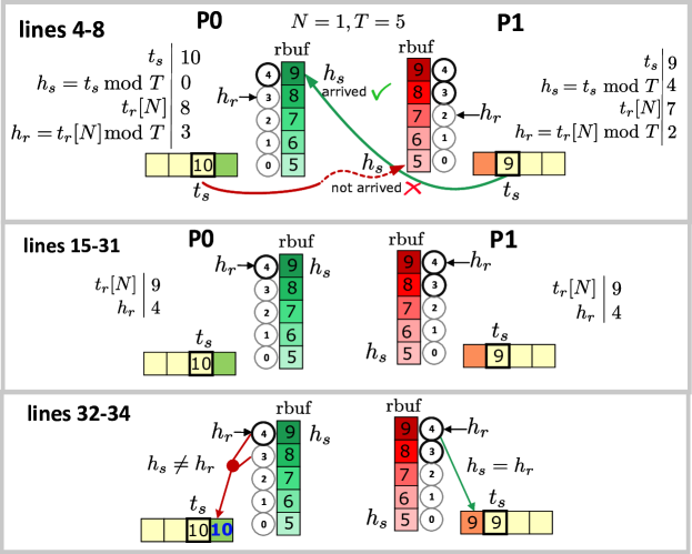
Figure 4: The processes P0 and P1 communicate using the weakly-synchronous halo exchange algorithm: the write of P1 completes while P0 just starts writing (lines 4-8), both P0 and P1 consume the notifications and advance the receive heads (lines 15-31), and finally P0 and P1 update the halo points using the latest available data (lines 32-34).

Figure 4 illustrates halo exchange communication. The processes P0 and P1 execute the time steps 10 and 9 which are composed of three main phases: 1) the processes write the halo points of the current time level to the corresponding entry in the circular buffer of the neighbor process, 2) the processes P0 and P1 consume the notifications and advance the receive heads accordingly, and 3) the processes P0 and P1 update the halo points using the data at the receive head. The process P1 copies the up-to-date data, while the process P0 approximates the halo points using two time levels.

We again tune the performance by hoisting the pack and approximation logic to OpenMP parallel loops. We also vary the start direction of the send and synchronization loops in round-robin fashion to avoid directional synchronization bias.

6 Results

In this section, we evaluate performance of the proposed weakly-synchronous (WS) algorithm against the traditional-synchronous (TS) algorithm. Before presenting the results on numerical accuracy and computational performance, we will briefly describe the simulation parameters and methodology used to obtain the results.

6.1 Setup and Methodology

To benchmark the algorithms, we developed a mini-application that solves the governing equations. The code is written in Fortran90 and parallelized with a hybrid OpenMP-MPI model. The experimental evaluation was performed on the GPU partition of the Piz Daint supercomputer at the Swiss National Supercomputing Center CSCS. The Cray XC50 connects 4400 nodes each with 1 Xeon E5-2690 v3 CPU and 1 Tesla P100 GPU using an Aries network interconnect with Dragonfly topology. All experiments launch 1 MPI process and 12 OpenMP threads per node, which fully utilizes the 12-core CPU while the GPU remains idle. We compile our code with gfortran 6.2 and use the foMPI-NA-0.2.4 (NA) and mpich2-1.2.1 (NB) libraries to implement the communication.

For the evaluation of numerical accuracy, simulations at different grid resolution are computed to a same end time of the solution. Unlike TS algorithm, which result in a unique solution for a given set of numerical and simulation parameters, the accuracy in the case of the WS algorithm is expected to vary with repetitions of the same experiment. This is due to the variability in the function time delay at halo points. Hence, we repeat each experiment 15 times in different allocations. A constant maximum allowable delay of $L=10$ has been used in the simulations of the WS algorithm.

For the computational performance experiments, we first execute 30 warm-up time steps and then 1000 time steps in a steady state for the measurements. The warm-up steps are required to populate the circular buffers of the WS algorithm. Again, a constant maximum allowable delay of $L=10$ is used in the case of WS algorithm simulations. As compute and communication times are commonly affected by system noise, we repeat each experiment 15 times in different allocations, as performed in the numerical accuracy experiments. We report median values and visualize the lower and upper quartiles using error bars.

6.2 Numerical Accuracy

In Figure 2 and Section 3.2, we have demonstrated the formal accuracy of the numerical method by showing the convergence of error in the computed solution obtained from the simulations of the linear advection-diffusion equation. Due to non-linearity in the advection term, the equations governing Burgers’ turbulence do not possess a simple analytical solution to compute the error. We, therefore, evaluate the numerical accuracy of the WS algorithm by comparing its solutions against the TS algorithm solution.

The asynchronous computations can introduce large errors at the process boundaries due to delayed function values in the stencil. However, the use of AT schemes at the process boundaries improves the numerical properties and restricts the error to remain within the order of accuracy. To examine the affects of asynchrony, instantaneous contours of the velocity component $u_{1}$ in a 2D plane obtained from the two algorithms using notified access communications are shown in Figure 5. The grid resolution is ${N}^{3}={120}^{3}$ and 3 MPI processes along each dimension have been used in the simulations. The multi-scale nature of the solution is evident from the contours. In comparison with the TS algorithm solution, the WS algorithm solution does not exhibit any noticeable aberrations either at the process boundaries, where the error due to asynchrony is introduced, or in the interior regions of the sub-domains, where the asynchrony error is expected to propagate with time.

Figure 5: Instantaneous conoturs of velocity component $u_{1}$ obtained from simulations using the (a) TS and (b) WS algorithms. The dashed black lines represent the process boundaries associated with the domain decomposition.

Figure 6: Variation of second central moment of (a) velocity component $u_{1}$ and (b) velocity-gradients component $\partial u_{1}/\partial x_{1}$ with grid count $N$. Blue-squares and red-circles are obtained from TS and WS algorithms, respectively. The error bars in red-circles represent the variability in values among different runs.

A grid convergence study is performed, which is a common practice in computational fluid dynamics, is performed to qualitatively assess the numerical accuracy. In such a study, values of key quantities of interest are computed at different grid counts. For a stable and an accurate numerical method, the error in the numerical solution decreases with an increase in the grid count. This results in the values of key quantities to asymptote to a constant value. In our experiments, we compute the convergence of moments of velocity and velocity gradients to study the effects of asynchrony on the accuracy of the WS algorithm. Figure 6 (a) and (b) show the grid convergence of the second moment of velocity component $u_{1}$ and its longitudinal gradient $\partial u_{1}/\partial x_{1}$, respectively. In the graphs, $N$ is the number of grid points in a given direction. With an increase in $N$ from $48$ to $240$, the number of hardware nodes have been increased from $1$ to $125$ in the simulations, which corresponds to a weak scaling of the problem with ${48}^{3}$ grid points per process. We observe that the moments in both the graphs converge to an asymptotic value for both TS (blue squares) as well as WS (red circles) algorithms. At the highest grid count the difference between the values from the two algorithms is less than $0.005\%$. The confidence intervals are shown for the moments from WS algorithm to show the effect of varying asynchrony among different simulation runs. The intervals show a very narrow spread at higher grid counts, which demonstrates that for a grid converged solution the results are insensitive to the degree of asynchrony. In these experiments, we have used a small set of simulation parameters ($L=10$, $P$ from $1$ to $125$) to evaluate the accuracy. It is very likely that the error in the solution would change for other simulation parameters. With an increase in $L$, the AT schemes at process boundaries will keep the error bounded as long as the overall numerical method remains stable [12, 13]. This study demonstrates that the WS algorithm provides an accurate solution for relaxed synchronization between processes.

6.3 Computational Performance

To study the performance and scalability, we evaluate the weakly-synchronous algorithm (WS) for different process/node counts and domain sizes, and compare its execution times to the traditional synchronous (TS) algorithm. Two sets of experiments examine strong and weak scaling for configurations relevant on future exascale systems and for setups that are commonly used today. The configurations scale the sub-domain size down to ${12}^{3}$ and ${24}^{3}$ grid points per process and compute on up to ${120}^{3}$ and ${240}^{3}$ grid points in total. The smallest configuration assigns $12^{2}$ grid points to every thread. As shown in Figure 7, this extreme scaling has comparable computation and communication times, and therefore fully utilizes the costly interconnect and compute hardware.

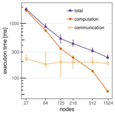
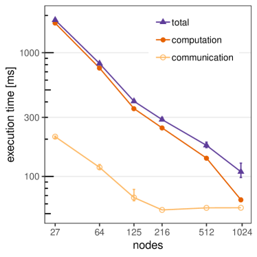
Figure 7: Scaling of computation, communication and total simulation times for (a) TS algorithm and (b) WS algorithm using notified access communication model in a strong scaling exercise with a problem size of ${120}^{3}$.

First, we present results from the strong scaling experiments. Figure 7 shows the computation, communication and total simulation times for a problem size of ${120}^{3}$. The runs decompose the domain evenly along all dimensions, resulting in cubical sub-domains. The process count is increased from $27$ to $1000$. Part (a) of the figure is obtained from the TS-NA algorithm. As the process count increases, the number of grid points per process decreases, and hence the computation time steadily reduces. Although the communication volume per process also decreases with the process count, the communication time remains nearly constant due to increasing synchronization cost and overwhelms the computation time above $250$ processes. A significant contribution to the total time is observed starting from $125$ processes, resulting in a poor scalability. The error bars in the graph indicate a substantial variability in communication time due to system noise among different runs, particularly at intermediate process counts. This variability also propagates into the total time, however to a lesser extent. Results from the WS algorithm are shown in Figure 7 (b). As the computational part of the code remains the same, the measured computation time remains unchanged compared to the TS algorithm. On the other hand, the communication time is significantly lower for the WS algorithm, with a speedup of 3.3x at the extreme scale. This is due to the relaxed synchronization that also dampens the performance variability. As a result, the bandwidth rather than the latency of the interconnect limits the communication performance of the WS algorithm. As the communication time does not exceed the computation time, a significant improvement in the scaling of the total time is observed.

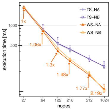
Figure 8: Strong scaling of ${120}^{3}$ problem size. TS: traditional-synchronous algorithm, WS: weakly-synchronous algorithm, NA: one-sided notified access communication model, NB: two-sided non-blocking communication model.

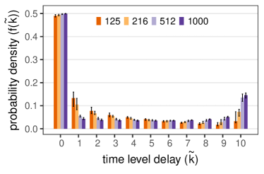
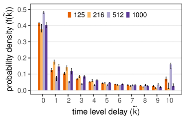
Figure 9: Distribution of delay in time level (${\tilde{k}}$) in WS algorithm simulations for a problem size of ${120}^{3}$ at different node counts. (a) WS algorithm with one-sided notified access communication model, (b) WS algorithm with two-sided non-blocking communication model.

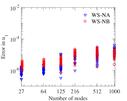
Figure 10: Average error in $u_{1}$ component of velocity from the weakly-synchronous (WS) algorithm computed against the synchronous solution for different runs in the strong scaling experiments of ${120}^{3}$ grid points problem size. Triangles and circles are from the simulations with one-sided notified access (NA) and two-sided non-blocking (NB) communication models, respectively.

The overall strong scaling of the two algorithms in combination with the two communication models for ${120}^{3}$ grid problem size is shown in Figure 8. Clearly, the WS algorithm outperforms the TS algorithm with a maximum speed up of $2.19$x at the extreme scale. The one-sided notified access communication model provides an additional minor improvement in the scaling. For the WS algorithm, the distribution of time delay in the function value experienced at the buffer points (${\tilde{k}}$) for the two communication models is presented in Figure 9. As discussed earlier, moments of the distribution of ${\tilde{k}}$ effect the accuracy of simulations. The figure shows that a better distribution with lower mean and variance is obtained with the NA communication model. Also the spread in the distributions across different runs is also lower for the NA communication model. To further assess the accuracy of solution, we compute the error in each of the WS algorithm runs by comparing its solution with the synchronous solution. Figure 10 shows the average error in the $u_{1}$ component of velocity for the runs at different node counts. It can be inferred that the NA communication model, due to a better distribution of the delays, provides relatively lower error values.

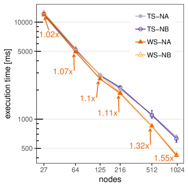
Figure 11: Strong scaling of ${240}^{3}$ problem size. TS: traditional-synchronous algorithm, WS: weakly-synchronous algorithm, NA: one-sided notified access communication model, NB: two-sided non-blocking communication model.

The strong scaling of a larger problem size with a grid of ${240}^{3}$ is illustrated in Figure 11. The WS algorithm continues to outperform the TS algorithm. However, the speed up at the extreme scale decreases to $1.55$x. This can be attributed to the increase in computational effort per process, and nearly the communication. A marginal gain is observed due to the NA communication model.

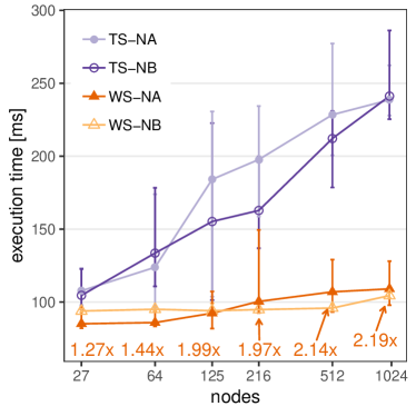
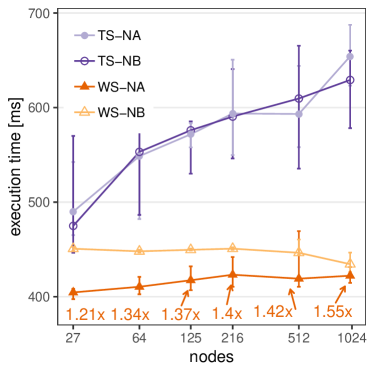
Figure 12: Weak scaling of (a) ${12}^{3}$ and (b) ${24}^{3}$ grid points per process. TS: traditional-synchronous algorithm, WS: weakly-synchronous algorithm, NA: one-sided notified access communication model, NB: two-sided non-blocking communication model.

The results from the weak scaling for ${12}^{3}$ and ${24}^{3}$ grid points per process are shown in Figure 12. The runs again decompose the domain evenly along all dimensions, which expands the overall compute domain from ${36}^{3}$ to ${120}^{3}$ and from ${72}^{3}$ to ${240}^{3}$ for the two configurations. The execution time for the WS algorithm remains nearly constant, while it significantly increases for the TS algorithm. This shows that WS algorithm is able to fully overlap the communications with computations. A speed up from $1.27$x to $2.19$x and $1.21$x to $1.55$x are observed in the ${12}^{3}$ and ${24}^{3}$ grid points per process configurations, respectively. The weak scaling also shows that the WS algorithm possess a lesser spread in the execution times among different runs. This demonstrates the robustness of the algorithm to system noise, consistent with our finding in the strong scaling.

7 Related Work

This work describes an asynchronous computing approach for solving PDEs, which uses an explicit time discretization for time derivatives. This relieves the need to solve a system of linear algebraic equations. However, certain classes of problems are governed by PDEs that are stiff in nature. Such PDEs are commonly solved with implicit time integration schemes, which result in linear system of equations that have to be solved at each time advancement.

Asynchronous iterative solvers, which do not require synchronization at each iteration, are available in the literature for linear systems [18, 19]. In the context of solving PDEs, these methods are useful only when time-implicit schemes are used. Even in such cases computations of linear systems within a time step can proceed asynchronously, but it is still necessary to communicate the data and synchronize at the end of each step. This issue can be resolved by coupling the asynchronous solvers with the the weakly-synchronous algorithm for PDEs.

Asynchronous methods for PDEs have been earlier proposed in Amitai at al. [20, 21], but their treatment is restricted to parabolic PDEs. They use corrections based on Green’s function to account for the asynchrony at process boundaries. In more recent works [22, 23], relieving the affects of asynchrony in communication have been addressed by modifying the governing PDEs instead of the numerical method. They demonstrated mathematical feasibility of their method using simple PDEs, but did not evaluate the computational performance. Also, extending their work to complex equations seems to be difficult. Methods that address other issues like resiliency to system faults and noise have been proposed in [24, 25].

Multiple works discuss the technology aspects of implementing efficient halo exchange communication. Kjolstad et al. [26] avoid synchronization using the non-blocking interface of two-sided MPI. Gropp et al. [27] demonstrate the benefits of one-sided MPI on platforms with native hardware support. Szpindler [28] compares the performance of different one-sided and two-sided implementations and obtains promising results for the foMPI-NA based version.

8 Conclusions

At extreme scales, data communication and synchronization between PEs significantly affect the scalability of parallel solvers. On future exascale machines which would be comprised of millions of PEs, these issues will certainly amplify further, and are likely to pose a bottleneck in designing scalable solvers. In an effort to relax synchronization and minimize communication costs in PDE solvers, we proposed a novel weakly-synchronous (WS) algorithm based on a mathematically asynchronous numerical method, where computations at processes can advance regardless of the status of communications. The numerical method uses new asynchrony-tolerant (AT) schemes that maintain the accuracy of the computed solution in presence of data asynchrony. However, these schemes pose three algorithmic requirements, namely: (a) synchronize communications between processes only when the delay between them is greater than the maximum allowable delay, (b) storage of data from multiple time levels or iterations at buffer points, and (c) knowledge of the time level associated with each communication. The WS algorithm addresses these requirements with minimal computation and communication overhead. The algorithm uses an efficient notified remote memory access programming model to implement communication between processes. The relaxed synchronization between processes naturally leads to a computation-communication overlap and has the potential to relieve the effects of system noise.

The performance of the WS algorithm is shown in comparison with traditional synchronous (TS) algorithm. We have developed a mini-application that simulates the multi-scale Burgers’ turbulence phenomena for the benchmark experiments. We use numerical schemes that provide an overall second order accuracy of solution in space. The algorithm implementation would remain similar for higher order accurate methods. The results from the numerical experiments show that the accuracy of the solution in WS algorithm are marginally affected due to data asynchrony. The WS algorithm provides a significant speed up over the synchronous algorithm. A speed up of 2.19x has been observed at extreme scales. The WS algorithm is also shown to be more robust to system noise. The performance evaluation of the WS algorithm clearly exhibits the potential for designing highly scalable PDE solvers for future exascale machines.

References

- Donzis and Jagannathan [2013] D. A. Donzis, S. Jagannathan, Fluctuations of thermodynamic variables in stationary compressible turbulence, J. Fluid Mech. 733 (2013) 221–244.
- Donzis et al. [2014] D. A. Donzis, K. Aditya, K. R. Sreenivasan, P. K. Yeung, The turbulent schmidt number, J. Fluids Eng. 136 (2014) 060912–060912.
- Minamoto and Chen [2016] Y. Minamoto, J. H. Chen, DNS of a turbulent lifted DME jet flame, Combustion and Flame 169 (2016) 38 – 50.
- Lee et al. [2013] M. Lee, N. Malaya, R. D. Moser, Petascale direct numerical simulation of turbulent channel flow on up to 786k cores, in: Proceedings of the International Conference on High Performance Computing, Networking, Storage and Analysis, SC ’13, ACM, New York, NY, USA, 2013, pp. 61:1–61:11.
- Ballard et al. [2010] G. Ballard, J. Demmel, O. Holtz, O. Schwartz, Communication-optimal parallel and sequential cholesky decomposition, SIAM Journal on Scientific Computing 32 (2010) 3495–3523.
- Grigori et al. [2008] L. Grigori, J. W. Demmel, H. Xiang, Communication avoiding gaussian elimination, in: Proceedings of the 2008 ACM/IEEE Conference on Supercomputing, SC ’08, IEEE Press, Piscataway, NJ, USA, 2008, pp. 29:1–29:12.
- Donfack et al. [2014] S. Donfack, S. Tomov, J. Dongarra, Dynamically balanced synchronization-avoiding lu factorization with multicore and gpus, in: Proceedings of the 2014 IEEE International Parallel & Distributed Processing Symposium Workshops, IPDPSW ’14, IEEE Computer Society, Washington, DC, USA, 2014, pp. 958–965.
- MPI Forum [????] MPI Forum, MPI: A message-passing interface standard. version 3, ????
- Dotsenko [2007] Y. Dotsenko, Expressiveness, programmability and portable high performance of global address space languages, ProQuest, 2007.
- Hoefler et al. [2010] T. Hoefler, T. Schneider, A. Lumsdaine, Characterizing the Influence of System Noise on Large-Scale Applications by Simulation, in: International Conference for High Performance Computing, Networking, Storage and Analysis (SC’10).
- Shalf et al. [2011] J. Shalf, S. Dosanjh, J. Morrison, Exascale computing technology challenges, in: Proceedings of the 9th International Conference on High Performance Computing for Computational Science, VECPAR’10, Springer-Verlag, Berlin, Heidelberg, 2011, pp. 1–25.
- Donzis and Aditya [2014] D. A. Donzis, K. Aditya, Asynchronous finite-difference schemes for partial differential equations, J. Comp. Phys. 274 (2014) 370 – 392.
- Aditya and Donzis [2017] K. Aditya, D. A. Donzis, High-order asynchrony-tolerant finite difference schemes for partial differential equations, Journal of Computational Physics 350 (2017) 550 – 572.
- Aditya and Donzis [2012] K. Aditya, D. A. Donzis, Poster: Asynchronous computing for partial differential equations at extreme scales, in: Proceedings of the 2012 SC Companion: High Performance Computing, Networking Storage and Analysis, SCC ’12, IEEE Computer Society, Washington, DC, USA, 2012, p. 1444.
- Aditya et al. [2018] K. Aditya, A. Gruber, C. Xu, T. Lu, A. Krisman, M. R. Bothien, J. H. Chen, Direct numerical simulation of flame stabilization assisted by autoignition in a reheat gas turbine combustor, Proceedings of the Combustion Institute (2018).
- Hoefler and Lumsdaine [2008] T. Hoefler, A. Lumsdaine, Message progression in parallel computing-to thread or not to thread?, in: Cluster Computing, 2008 IEEE International Conference on, IEEE, pp. 213–222.
- Belli and Hoefler [2015] R. Belli, T. Hoefler, Notified Access: Extending Remote Memory Access Programming Models for Producer-Consumer Synchronization, in: Proceedings of the 29th IEEE International Parallel & Distributed Processing Symposium (IPDPS’15), IEEE, 2015.
- Bertsekas and Tsitsiklis [1989] D. P. Bertsekas, J. N. Tsitsiklis, Parallel and distributed computation, 1989.
- Frommer and Szyld [2000] A. Frommer, D. B. Szyld, On asynchronous iterations, Journal of computational and applied mathematics 123 (2000) 201–216.
- Amitai et al. [1996] D. Amitai, A. Averbuch, M. Israeli, S. Itzikowitz, On parallel asynchronous high-order solutions of parabolic PDEs, Numer. Algorithms 12 (1996) 159–192.
- Amitai et al. [1998] D. Amitai, A. Averbuch, M. Israeli, S. Itzikowitz, Implicit-explicit parallel asynchronous solver of parabolic PDEs, SIAM J. Sci. Comput. 19 (1998) 1366–1404.
- Mudigere et al. [2014] D. Mudigere, S. D. Sherlekar, S. Ansumali, Delayed difference scheme for large scale scientific simulations, Physical review letters 113 (2014) 218701.
- Mittal and Girimaji [2016] A. Mittal, S. Girimaji, ’proxy-equation’paradigm-a novel strategy for massively-parallel asynchronous computations, arXiv preprint arXiv:1611.04985 (2016).
- Sargsyan et al. [2015] K. Sargsyan, F. Rizzi, P. Mycek, C. Safta, K. Morris, H. Najm, O. L. Maître, O. Knio, B. Debusschere, Fault resilient domain decomposition preconditioner for PDEs, SIAM Journal on Scientific Computing 37 (2015) A2317–A2345.
- Grout et al. [2015] R. W. Grout, H. Kolla, M. L. Minion, J. B. Bell, Achieving algorithmic resilience for temporal integration through spectral deferred corrections, arXiv preprint arXiv:1504.01329 (2015).
- Kjolstad and Snir [2010] F. B. Kjolstad, M. Snir, Ghost cell pattern (2010).
- Gropp and Thakur [2007] W. D. Gropp, R. Thakur, Revealing the performance of MPI RMA implementations, in: European Parallel Virtual Machine/Message Passing Interface Users’ Group Meeting, Springer, pp. 272–280.
- Szpindler [2016] M. Szpindler, Scalable remote memory access halo exchange with reduced synchronization cost, in: Proceedings of Cray User Group (CUG) Conference.