Integer Programming Approaches to
Balanced Connected $k$-Partition

Abstract

We address the problem of partitioning a vertex-weighted connected graph into $k$ connected subgraphs that have similar weights, for a fixed integer $k\geq 2$. This problem, known as the balanced connected $k$-partition problem ($\textsc{BCP}_{k}$), is defined as follows. Given a connected graph $G$ with nonnegative weights on the vertices, find a partition $\{V_{i}\}_{i=1}^{k}$ of $V(G)$ such that each class $V_{i}$ induces a connected subgraph of $G$, and the weight of a class with the minimum weight is as large as possible. It is known that $\textsc{BCP}_{k}$ is ${NP}$-hard even on bipartite graphs and on interval graphs. It has been largely investigated under different approaches and perspectives. On the practical side, $\textsc{BCP}_{k}$ is used to model many applications arising in police patrolling, image processing, cluster analysis, operating systems and robotics. We propose three integer linear programming formulations for the balanced connected $k$-partition problem. The first one contains only binary variables and a potentially large number of constraints that are separable in polynomial time. Some polyhedral results on this formulation, when all vertices have unit weight, are also presented. The other formulations are based on flows and have a polynomial number of constraints and variables. Preliminary computational experiments have shown that the proposed formulations outperform the other formulations presented in the literature.

Keywords: connected partition, mixed integer linear programming, polyhedra, facet.

1 Introduction

The graphs considered here are simple, connected and undirected. If $G$ is a graph, then $V(G)$ denotes its vertex set and $E(G)$ denotes its edge set. Later, for some formulations, we shall refer to directed graphs (or simply, digraphs) $D$, with vertex set $V(D)$ and arc set $A(D)$. For an integer $k\geq 1$, as usual, the symbol $[k]$ denotes the set $\{1,2,\dots,k\}$. Throughout this text, $k$ denotes a positive integer number.

Let $G$ be a connected graph. A $k$-partition of $G$ is a collection $\{V_{i}\}_{i\in[k]}$ of nonempty subsets of $V(G)$ such that $\bigcup_{i=1}^{k}V_{i}=V(G)$, and $V_{i}\cap V_{j}=\emptyset$ for all $i,j\in[k]$, $i\neq j$. We refer to each set $V_{i}$ as a class of the partition. In this context, we assume that $|V(G)|\geq k$, otherwise $G$ does not admit a $k$-partition. We say that a $k$-partition $\{V_{i}\}_{i\in[k]}$ of $G$ is connected if $G[V_{i}]$, the subgraph of $G$ induced by $V_{i}$, is connected for each $i\in[k]$. Let $w\colon V(G)\to\mathbb{Q}_{>}$ be a function that assigns weights to the vertices of $G$. For every subset $V^{\prime}\subseteq V(G)$, we define $w(V^{\prime})=\sum_{v\in V^{\prime}}w(v)$. To simplify notation, we write $w(H)=w(V(H))$ when $H$ is a graph. In the balanced connected $k$-partition problem ($\textsc{BCP}_{k}$), we are given a vertex-weighted connected graph, and we seek a connected $k$-partition such that the weight of a lightest class of this partition is maximized. A more formal definition of this problem is given below, as well as an example of an instance for $\textsc{BCP}_{2}$ (see Figure 1). For some fixed positive integer $k$, each input of $\textsc{BCP}_{k}$ is given by a pair $(G,w)$. We denote by $\operatorname{\rm{OPT}}_{k}(G,w)$ the weight of a lightest set in an optimal connected $k$-partition of $V(G)$; but write simply $\operatorname{\rm{OPT}}(G,w)$ when $k$ is clear from the context. Furthermore, we simply denote by $G$ the instance in which $w$ is an assignment of a constant value to all vertices (which we may assume to be $1$).

Problem 1.

Balanced Connected $k$-Partition ($\textsc{BCP}_{k}$)
Instance: a connected graph $G$ and a vertex-weight function $w\colon V(G)\to\mathbb{Q}_{>}$.
Find: a connected $k$-partition $\{V_{i}\}_{i\in[k]}$ of $V(G)$.
Goal: maximize $\min_{i\in[k]}(w(V_{i}))$.

(a) A vertex-weighted graph.

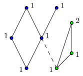
(b) Optimal solution of cost 4. The dashed edge links vertices of different classes.

Figure 1: An instance for $\textsc{BCP}_{2}$ and its optimal solution

There are several problems in police patrolling, image processing, data base, operating systems, cluster analysis, education and robotics that can be modeled as a balanced connected partition problem [2, 14, 15, 16, 17, 22]. These different real-world applications indicate the importance of designing algorithms for $\textsc{BCP}_{k}$, and reporting on the computational experiments with their implementations. Not less important are the theoretical studies of the rich and diverse mathematical formulations and the polyhedral investigations $\textsc{BCP}_{k}$ leads to.

Let us denote by $\textsc{1-BCP}_{k}$ the restricted version of $\textsc{BCP}_{k}$ in which all vertices have unit weight. One may easily check that $\textsc{1-BCP}_{2}$ on 2-connected graphs can be solved in polynomial time. This problem also admits polynomial-time algorithms on graphs such that each block has at most two articulation vertices [1, 5, 10, 11]. Dyer and Frieze [8] showed that, for every $k\geq 2$,  $\textsc{1-BCP}_{k}$ is ${NP}$-hard on bipartite graphs. Wu [21] proved that $\textsc{BCP}_{k}$ is ${NP}$-hard even on interval graphs, for all $k\geq 2$.

For the $\textsc{BCP}_{2}$ (weighted version), Chlebíková [5] showed that this problem is ${NP}$-hard to approximate within an absolute error guarantee of $|V(G)|^{1-\varepsilon}$, for all $\varepsilon>0$. In that same paper, Chlebíková designed a $4/3$-approximation algorithm for that problem. For $\textsc{BCP}_{3}$ and $\textsc{BCP}_{4}$ on $3$-connected and $4$-connected graphs, respectively, there exist $2$-approximation algorithms proposed by Chataigner et al. [4].

Wu [21] showed the first pseudo-polynomial algorithm for $\textsc{BCP}_{2}$ restricted to interval graphs. Based on this algorithm and using a scaling technique, Wu obtained a $(1+\varepsilon)$-approximation with running time $\mathcal{O}((1+1/\varepsilon)n^{3})$, where $n$ is the number of vertices of the input graph.

Borndörfer et al. [3] designed a $\Delta$-approximation for $\textsc{BCP}_{k}$, where $\Delta$ is the maximum degree of an arbitrary spanning tree of the given graph. This is the first known approximation algorithm on general graphs.

Mixed integer linear programming (MILP) formulations were proposed for $\textsc{BCP}_{2}$ by Matic [18] and for $\textsc{BCP}_{k}$ by Zhou et al. [22]. Additionally, Matic presented an heuristic algorithm based on a variable neighborhood search (VNS) technique for $\textsc{BCP}_{2}$, and Zhou et al. devised a genetic algorithm for $\textsc{BCP}_{k}$. In both works, the authors showed results of computational experiments to illustrate the quality of the solutions constructed by the proposed heuristics and their running times compared to the exact algorithms based on the MILP formulations. No polyhedral study of their formulations was reported.

This paper is organized as follows. In Section 2, we present a natural cut formulation for $\textsc{BCP}_{k}$ and also two stronger valid inequalities for this formulation. A further polyhedral study of this formulation, when all vertices have unit weight, is presented in Section 3. Two of the inequalities in the formulation are shown to define facets, and one of them is characterized when it is facet-defining. In Section 4, we present a flow and a multicommodity flow based formulations for $\textsc{BCP}_{k}$. In Section 5, we report on the computational experiments with our formulations and also with those presented by Matic [18] and Zhou et al. [22]. We summarize our theoretical and practical contributions for $\textsc{BCP}_{k}$ in Section 6.

2 Cut formulation

In this section, the following concept will be useful. Let $u$ and $v$ be two non-adjacent vertices in a graph $G$. We say that a set $S\subseteq V(G)\setminus\{u,v\}$ is a $(u,v)$-separator if $u$ and $v$ belong to different components of $G-S$. We define $\Gamma(u,v)$ as the collection of all minimal $(u,v)$-separators in $G$.

Let $(G,w)$ be an input for $\textsc{BCP}_{k}$. We propose the following natural integer linear programming formulation $\mathcal{C}_{k}(G,w)$ for $\textsc{BCP}_{k}$. For that, for every vertex $v\in V(G)$ and $i\in[k]$, we define a binary variable $x_{v,i}$ representing that $v$ belongs to the $i$-th class if and only if $x_{v,i}=1$. In this formulation, to get hold of a class with the smallest weight, we impose an ordering of the classes, according to their weights, so that the first class becomes the one whose weight we want to minimize.

$$\max\> \sum_{v\in V(G)}w(v)\>x_{v,1}$$

s.t. $$\sum_{v\in V(G)}w(v)\>x_{v,i}\leq\sum_{v\in V(G)}w(v)\>x_{v,i+1} \!\!\!\!\!\!\forall v\in V(G),i\in[k-1],$$ (1)

$$\sum_{i\in[k]}x_{v,i}\leq 1 \!\!\!\!\!\!\forall v\in V(G),$$ (2)

$$x_{u,i}+x_{v,i}-\sum_{z\in S}x_{z,i}\leq 1 \!\!\!\!\!\!\forall uv\notin E(G),S\in\Gamma(u,v),i\in[k],$$ (3)

$$x_{v,i}\in\{0,1\} \!\!\!\!\!\!\forall v\in V(G)\text{ and }i\in[k].$$ (4)

Inequalities (1) imply a non-decreasing weight ordering of the classes. Inequalities (2) impose that every vertex is assigned to at most one class. Inequalities (3) guarantee that every class induces a connected subgraph. The objective function maximizes the weight of the first class. Thus, in an optimal solution no class will be empty, and therefore it will always correspond to a connected $k$-partition of $G$.

We observe that the separation problem associated with inequalities (3) can be solved in polynomial time by reducing it to the minimum cut problem. Thus, the linear relaxation of $\mathcal{C}_{k}$ can be solved in polynomial time because of the equivalence of separation and optimization (see [12]).

Since the feasible solutions of the formulation above may have empty classes, to refer to these solutions we introduce the following concept. A connected $k$-subpartition of $G$ is a connected $k$-partition of a subgraph (not necessarily proper) of $G$. Henceforth, we assume that if  $\mathcal{V}=\{V_{i}\}_{i=1}^{k}$ is a connected $k$-subpartition of $G$, then $w(V_{i})\leq w(V_{i+1})$ for all $i\in[k-1]$. For such a $k$-subpartition $\mathcal{V}$, we denote by $\xi(\mathcal{V})\in\mathbb{B}^{nk}$ the binary vector such that its non-null entries are precisely $\xi(\mathcal{V})_{v,i}=1$ for all $i\in[k]$ and $v\in V_{i}$ (that is, $\xi(\mathcal{V})$ denotes the incidence vector of $\mathcal{V}$).

We next show that the previous formulation correctly models $\textsc{BCP}_{k}$. For that, let $\mathcal{P}_{k}(G,w)$ be the polytope associated with that formulation, that is,

$$\mathcal{P}_{k}(G,w)=\operatorname{\rm{convex-hull}}\{x\in\mathbb{B}^{nk}\colon x\text{ satisfies inequalities }\eqref{ineq:asymetric}-\eqref{ineq:cut}\text{ of }\mathcal{C}_{k}(G,w)\}.$$

In the next proposition we show that $\mathcal{P}_{k}(G,w)$ is the convex hull of the incidence vectors of connected $k$-subpartitions of $G$.

Proposition 1.

Let $(G,w)$ be an input for $\textsc{BCP}_{k}$. Then, the following holds.

$$\mathcal{P}_{k}(G,w)=\operatorname{\rm{convex-hull}}\{\xi(\mathcal{V})\in\mathbb{B}^{nk}\colon\mathcal{V}\text{ is a connected $k$-subpartition of }G\}.$$

Proof.

Consider first an extreme point $x\in\mathcal{P}_{k}(G,w)$. For each $i\in[k]$, we define the set of vertices $U_{i}=\{v\in V(G)\colon x_{v,i}=1\}$. It follows from inequalities (1) and (2) that $\mathcal{U}:=\{U_{i}\}_{i=1}^{k}$ is a $k$-subpartition of $G$ such that $w(U_{i})\leq w(U_{i+1})$ for all $i\in[k-1]$.

To prove that $\mathcal{U}$ is a connected $k$-subpartition, we suppose to the contrary that there exists $i\in[k]$ such that $G[U_{i}]$ is not connected. Hence, there exist vertices $u$ and $v$ belonging to two different components of $G[U_{i}]$. Moreover, there is a minimal set of vertices $S$ that separates $u$ and $v$ and such that $S\cap U_{i}=\emptyset$. This implies that $x_{v,i}+x_{u,i}-\sum_{z\in S}x_{z,i}=x_{v,i}+x_{u,i}=2$, a contradiction to the fact that  $x$ satisfies inequalities (3). Therefore, $\mathcal{U}$ is a connected $k$-subpartition of $G$.

To show the converse, consider now a connected $k$-subpartition $\mathcal{V}=\{V_{i}\}_{i=1}^{k}$ of $G$. By the definition of $\xi(\mathcal{V})$, it is clear that this vector satisfies inequalities (1) and (2). Take a fixed $i\in[k]$. For every pair  $u$,$v$ of non-adjacent vertices in $V_{i}$, and every $(u,v)$-separator $S$ in $G$, it holds that $S\cap V_{i}\neq\emptyset$, because  $G[V_{i}]$ is connected. Therefore, $\xi(\mathcal{V})$ satisfies inequalities (3). Consequently, $\xi(\mathcal{V})$ belongs to $\mathcal{P}_{k}(G,w)$. ∎

In the remainder of this section we present two further classes of valid inequalities for $\mathcal{P}_{k}(G,w)$ that strenghten the formulation $\mathcal{C}_{k}(G,w)$. We start showing a class that dominates the class of inequalities (3).

Proposition 2.

Let $(G,w)$ be an input for $\textsc{BCP}_{k}$. Let $u$ and $v$ be two non-adjacent vertices of $G$, and let $S$ be a minimal $(u,v)$-separator. Let $L=\left\{z\in S\colon w(P_{z})>\frac{w(G)}{k-i+1}\right\}$, where $P_{z}$ is a minimum-weight path between $u$ and $v$ in $G$ that contains $z$. For every $i\in[k]$, the following inequality is valid for $\mathcal{P}_{k}(G,w)$:

$$x_{u,i}+x_{v,i}-\sum_{z\in S\setminus L}x_{z,i}\leq 1.$$ (5)

Proof.

Consider an extreme point $x$ of $\mathcal{P}(G,w)$, and define $V_{i}=\{v\in V(G)\colon x_{v,i}=1\}$ for each $i\in[k]$. Suppose to the contrary that there is $j\in[k]$ such that $w(V_{j})>\frac{w(G)}{k-j+1}$. Since $x$ satisfies inequalities (1), it holds that $\sum_{i\in[k]\setminus[j-1]}w(V_{i})>w(G)$, a contradiction. Thus, if $u$ and $v$ belong to $V_{i}$, then there exists a vertex $z\in S\setminus L$ such that $z$ also belongs to $V_{i}$. Therefore, $x$ satisfies inequality (5). ∎

Inspired by the inequalities devised by de Aragão and Uchoa [6] for a connected assignment problem, we propose the following class of inequalities for $\mathcal{P}_{k}(G,w)$.

Proposition 3.

Let $(G,w)$ be an input for $\textsc{BCP}_{k}$, and $q\geq 2$ be an integer. Let $S$ be a subset of $V(G)$, $N(S)$ the set of neighbors of $S$, and  $S^{\prime}$ a subset of $S$ containing $q$ distinct pair of vertices $\{s_{i},t_{i}\}$, $s_{i}\neq t_{i}$, $i\in[q]$. Moreover, let $\sigma\colon[q]\to[k]$ be an injective function, and let $I$ denote the image of $\sigma$, that is, $I=\{\sigma(i)\in[k]\colon i\in[q]\}$. If there is no collection of $q$ vertex-disjoint $(s_{i},t_{i})$-paths in $G[S]$, then the following inequality is valid for $\mathcal{P}_{k}(G,w)$:

$$\sum_{i\in[q]}\left(x_{s_{i},\sigma(i)}+x_{t_{i},\sigma(i)}\right)+\sum_{v\in N(S)}\sum_{i\in[k]\setminus I}x_{v,i}\leq 2q+|N(S)|-1\enspace.$$ (6)

Proof.

Suppose, to the contrary, that there exists an extreme point $x$ of $\mathcal{P}_{k}(G,w)$ that violates inequality (6). Let $A=\sum_{i\in[q]}\left(x_{s_{i},\sigma(i)}+x_{t_{i},\sigma(i)}\right)$ and $B=\sum_{v\in N(S)}\sum_{i\in[k]\setminus I}x_{v,i}$. From inequalities (2), we have that $A\leq 2q$. Since $x$ violates (6), it follows that $B>|N(S)|-1$. Thus $B=|N(S)|$ (because $x$ satisfies inequalities (2)). Hence, every vertex in $N(S)$ belongs to a class that is different from those indexed by $I$. This implies that every class indexed by $I$ contains precisely one of the $q$ distinct pairs $\{s_{i},t_{i}\}$. Therefore, there exists a collection of $q$ vertex-disjoint $(s_{i},t_{i})$-paths in $G[S]$, a contradiction. ∎

Kawarabayashi et al. [13] proved that, given an $n$-vertex graph $G$ and a set of $q$ pairs of terminals in $G$, the problem of deciding whether $G$ contains $q$ vertex-disjoint paths linking the given pairs of terminals can be solved in time $\mathcal{O}(n^{2})$. Hence, inequalities (6) can be separated in polynomial time when $S=V(G)$.

3 Polyhedral results for $\textsc{1-BCP}_{k}$

In this section we focus on $\textsc{1-BCP}_{k}$, the special case of $\textsc{BCP}_{k}$ in which all vertices have unit weight. In this case, instead of $\mathcal{P}_{k}(G,w)$, we simply write $\mathcal{P}_{k}(G)$, the polytope defined as the convex hull of $\{x\in\mathbb{B}^{kn}:x\text{ satisfies }\eqref{ineq:asymetric}\text{ - }\eqref{ineq:cut}\}$.

Note that, if the input graph $G$ has no matching of size $k$, then $G$ has no feasible connected $k$-subpartition $\{V_{i}\}_{i\in[k]}$ such that $|V_{i}|\geq 2$ for all $i\in[k]$, and thus $\operatorname{\rm{OPT}}(G)=1$, and it is easy to find an optimal solution. Thus, we assume from now on that $G$ has a matching of size $k$ (a property that can be checked in polynomial time [9]), and that $n\geq 2k$, where $n:=|V(G)|$.

For each  $v\in V(G)$ and $i\in[k]$ we shall construct a binary vector $\chi(v,i)$ that belongs to $\mathcal{P}_{k}(G)$. Let us denote by $e(v,i)\in\mathbb{B}^{nk}$ the unit vector such that its single non-null entry is indexed by $v$ and $i$. Now consider any set $S\subseteq V(G)\setminus\{v\}$, $|S|=k-i$, and a bijective function $\nu\colon S\to[k]\setminus[i]$. Since $n\geq 2k$, such a set $S$ exists. Fix a pair $(S,\nu)$, where $S$ and $\nu$ are as previously defined. Let $\chi(v,i)\in\mathbb{B}^{nk}$ be the vector $e(v,i)+\sum_{u\in S}e(u,\nu(u))$. Note that $\chi(v,i)$ belongs to $\mathcal{P}_{k}(G)$, it is the incidence vector of a $k$-subpartition, say ${\mathcal{S}}_{i}=\{S_{i},\ldots,S_{k}\}$ of $G$, in which $v$ belongs to the class $S_{i}$, and each vertex of $S\subseteq V(G)\setminus\{v\}$ belongs to one of the classes $S_{i+1},\ldots,S_{k}$, all of which are singletons.

To be rigorous, we should write $\chi^{s,\nu}(v,i)$ as different choices of $S$ and $\nu$ give rise to different vectors, but we simply write $\chi(v,i)$ with the understanding that it refers to some $S$ and bijection $\nu$.

Proposition 4.

$\mathcal{P}_{k}(G)$ is full-dimensional, that is, $\dim(\mathcal{P}_{k}(G))=kn$.

Proof.

Let $X$ be the set of $kn$ vectors previously defined, that is,  $X=\{\chi(v,i)\in\mathbb{B}^{nk}\colon v\in V(G)\text{ and }i\in[k]\}$. Assume that $V(G)=\{v_{1},\ldots,v_{n}\}$. We suppose, with no loss of generality, that the indices of a vector $x$ in $X$ are ordered as $(x_{v_{1},1},\ldots,x_{v_{n},1},\ldots,x_{v_{1},k},\ldots,x_{v_{n},k})$.

Let $M$ be the matrix whose columns are precisely the $nk$ vectors in $X$ (in the following order): $\chi(v_{1},1),\ldots,\chi(v_{n},1),\ldots,\chi(v_{1},k),\ldots,\chi(v_{n},k)$. One may easily check that $M$ is a lower triangular square matrix of dimension $kn$. Note that the columns of $M$ are precisely the vectors in $X$. Hence the vectors in $X$ are linearly independent. Since $X\subseteq\mathcal{P}_{k}(G)$, we conclude that $\dim(\mathcal{P}_{k}(G))=nk$, that is, $\mathcal{P}_{k}(G)$ is full-dimensional. ∎

In the forthcoming proofs, we have to refer to some connected $k$-subpartitions of $G$, defined (not uniquely) in terms of distinct vertices $u$, $v$ of $G$, and specific classes $i$, $j$, where $i<j$. For that, we define a short notation to represent the incidence vectors of these connected $k$-subpartitions. Given such $u$, $v$, and $i$, $j$, choose two set of vertices $S$ and $\hat{S}$ in $G$, both of cardinality $k-i+1$, and bijections $\pi\colon S\to\{i,\ldots,k\}$ and $\hat{\pi}\colon\hat{S}\to\{i,\ldots,k\}$ such that

1. $u\in S\cap\hat{S}$ and $v\in S\setminus\hat{S}$;

2. $\pi(u)=\hat{\pi}(u)=i$ and $\pi(v)=j$.

Let $\phi(u,i,v,j)$ and $\psi(u,i,v)$ be vectors in $\{0,1\}^{nk}$ such that their non-null entries are precisely: $\phi(u,i,v,j)_{z,\pi(z)}=1$ for every $z\in S$, and $\psi(u,i,v)_{z,\hat{\pi}(z)}=1$ for every $z\in\hat{S}$. The vectors $\phi(u,i,v,j)$ and $\psi(u,i,v)$ clearly belong to $\mathcal{P}_{k}(G)$. Moreover, note that $\phi(u,i,v,j)_{u,i}=\phi(u,i,v,j)_{v,j}=\psi(u,i,v)_{u,i}=1$ and $\psi(u,i,v)_{v,\ell}=0$ for all $\ell\in[k]$.

Proposition 5.

For every $v\in V(G)$ and $i\in[k]$, the inequality $x_{v,i}\geq 0$ induces a facet of $\mathcal{P}_{k}(G)$.

Proof.

Similarly to the proof of Proposition 4, let $X_{1}=\{\chi(v,j)\in\mathbb{B}^{nk}\colon j\in[k]\setminus\{i\}\}$. Additionally, we define $X_{2}=\{\psi(u,j,v)\in\mathbb{B}^{nk}\colon u\in V(G)\setminus\{v\}\text{ and }j\in[k]\}$. Note that $|X_{1}\cup X_{2}|=nk-1$. Since the null vector and all vectors in $X_{1}\cup X_{2}$ are all affinely independent, and they all belong to the face $\{x\in\mathbb{B}^{nk}\colon x_{v,i}=0\}$, we conclude that the inequality $x_{v,i}\geq 0$ induces a facet of $\mathcal{P}_{k}(G)$. ∎

In what follows, considering that the polytope $\mathcal{P}_{k}(G)$ is full-dimensional, to prove that a face $\hat{F}=\{x\in\mathcal{P}_{k}(G)\colon\hat{\lambda}x=\hat{\lambda}_{0}\}$ is a facet of $\mathcal{P}_{k}(G)$, we show that if a nontrivial face $F=\{x\in\mathcal{P}_{k}(G)\colon\lambda x=\lambda_{0}\}$ of $\mathcal{P}_{k}(G)$ contains $\hat{F}$, then there exists a real positive constant $c$ such that $\lambda=c\hat{\lambda}$ and $\lambda_{0}=c\hat{\lambda}_{0}$.

Proposition 6.

For every $v\in V(G)$, the inequality $\sum_{i\in[k]}x_{v,i}\leq 1$ induces a facet of $\mathcal{P}_{k}(G)$.

Proof.

Fix a vertex $v\in V(G)$. Let $\hat{F}_{v}=\{x\in\mathcal{P}_{k}(G)\colon\hat{\lambda}x=\hat{\lambda}_{0}\}$, where $\hat{\lambda}x\leq\hat{\lambda}_{0}$ corresponds to $\sum_{i\in[k]}x_{v,i}\leq 1$. Let $F=\{x\in\mathcal{P}_{k}(G)\colon\lambda x=\lambda_{0}\}$ be a nontrivial face of $\mathcal{P}_{k}(G)$ such that $\hat{F}_{v}\subseteq F$. We shall prove that $\lambda_{v,i}=\lambda_{0}$ and $\lambda_{u,i}=0$ for every $u\in V(G)\setminus\{v\}$ and $i\in[k]$.

Since $G$ is nontrivial and connected, it is easy to see that $G$ has a set of $n$ nested connected subgraphs $G_{1},G_{2},\ldots,G_{n}$ such that $G_{1}$ consists solely of the vertex $v$, each $G_{j}\subset G_{j+1}$ for $j=2,\ldots n-1$, and $G_{n}=G$. (It suffices to consider a spanning tree in $G$, and starting from $v$, define the subsequent subgraphs by adding at each step an appropriate edge and vertex from this spanning tree.)

Consider the set of vectors $A=\{e(G_{j},k)\}_{j\in[n]}$, where $e(G_{j},k)=\sum_{u\in V(G_{j})}e(u,k)$ for every $j\in[n]$. Since $v\in V(G_{j})$ for all $j\in[n]$, it follows that $A\subseteq\hat{F}_{v}$. As a consequence, $\lambda_{u,k}=0$ for all $u\in V(G)\setminus\{v\}$. Additionally, $\lambda_{v,k}=\lambda_{0}$ since $e(v,k)\in\hat{F}_{v}$.

Let $\ell\in[k]\setminus\{1\}$. Suppose that $\lambda_{v,i}=\lambda_{0}$ and $\lambda_{u,i}=0$ for every $u\in V(G)\setminus\{v\}$ and $i\in\{\ell,\ldots,k\}$. Now define the set of vectors $B=\{\phi(u,\ell-1,v,k)\colon u\in V(G)\setminus\{v\}\}$. Note that $B\subseteq\hat{F}_{v}$, since $v$ belongs to exactly one class of the partition corresponding to each vector in $B$. By the induction hypothesis, we obtain $\lambda_{u,\ell-1}=0$ for each $u\in V(G)\setminus\{v\}$. Moreover, observe that $\chi(v,\ell-1)$ belongs to $\hat{F}_{v}$. It follows from the induction hypothesis that $\lambda(\chi(v,\ell-1))=\lambda_{v,\ell-1}=\lambda_{0}$.

Therefore, we conclude that $\lambda=\lambda\left(\sum_{i\in[k]}e(v,i)\right)=\lambda_{0}\hat{\lambda}$. Since $\lambda_{0}\neq 0$ (otherwise $F$ would be a trivial face), it follows that $\lambda x\leq\lambda_{0}$ is a multiple scalar of $\hat{\lambda}x\leq\hat{\lambda}_{0}$, and therefore $\hat{F}_{v}$ is a facet of $\mathcal{P}_{k}(G)$. ∎

Let $u$ and $v$ be two non-adjacent vertices of $G$ and let $S$ be a minimal $(u,v)$-separator in $G$. We denote by $H_{u}$ and $H_{v}$ the components of $G-S$ which contain $u$ and $v$, respectively. Since $S$ is minimal, it follows that every vertex in $S$ has at least one neighbor in $H_{u}$ and one in $H_{v}$.

In this context of minimal $(u,v)$-separator $S$, for every $z\in V(G)$, the following two concepts (and notation) will be important for the next result.

We denote by $G_{z}$ a minimum size connected subgraph of $G$ containing $z$, with the following properties: If $z\in V(H_{v})$, then $G_{z}$ is contained in $H_{v}$; if $z\in V(H_{u})$, then $G_{z}$ is contained in $H_{u}$. Otherwise, $G_{z}$ contains $u$, $v$ and exactly one vertex of $S$, that is, $|V(G_{z})\cap S|=1$. Clearly, such a subgraph always exists. Moreover, if $z\notin S\cup\{u,v\}$, then the subgraph $G_{z}-z$ is connected (that is, $z$ is not a cutvertex of $G_{z}$).

For any integer $i\in[k]$, we say that $G$ admits a $(u,v,S,i)$-robust subpartition if, for each $z\in V(G)\setminus\{u,v\}$, there is a connected $(k-i)$-subpartition $\{V_{j}\}_{j\in[k]\setminus[i]}$ of $G-G_{z}$ such that $|V(G_{z})|\leq|V_{j}|$ for all $j\in[k]\setminus[i]$.

Theorem 7.

Let $u$ and $v$ be non-adjacent vertices in $G$, let $S$ be a minimal $(u,v)$-separator, and let $i\in[k]$. Then $G$ admits a $(u,v,S,i)$-robust subpartition if and only if the following inequality induces a facet of $\mathcal{P}_{k}(G)$:

$$x_{u,i}+x_{v,i}-\sum_{s\in S}x_{s,i}\leq 1\enspace.$$

4 Flow formulations

We present in this section a mixed integer linear programming formulation for $\textsc{BCP}_{k}$ based on flows in a digraph. For that, given an input $(G,w)$ for $\textsc{BCP}_{k}$, we construct a digraph $D$ as follows: First, we add to $G$ a set $S=\{s_{1},\ldots,s_{k}\}$ of $k$ new vertices. Then, we replace every edge of $G$ with two arcs with the same endpoints and opposite directions. Finally, we add an arc from each vertex in $S$ to each vertex of $G$ (see Figure 2). More formally, the vertex set of $D$ is $V(D)=V(G)\cup S$ and its arc set is

$$A(D)=\{(u,v),(v,u):\{u,v\}\in E(G)\}\cup\{(s_{i},v):i\in[k],v\in V(G)\}.$$

Now, the idea behind the formulation is the following: find in $D$ a maximum flow from the $k$ sources in $S$ such that every vertex $v$ in $V(D)\setminus S$ receives flow only from a single vertex of $D$ and consumes $w(v)$ of the received flow. As we shall see, for every $i\in[k]$, the flow sent from source $s_{i}$ corresponds to the total weight of the vertices in the $i$-th class of the desired partition.

To model this concept, with each arc $a\in A(D)$, we associate a non-negative real variable $f_{a}$ that represents the amount of flow passing through $a$, and a binary variable $y_{a}$ that equals one if and only if arc $a$ is used to transport a positive flow. The corresponding formulation, shown below, is denoted $\mathcal{F}_{k}(G,w)$.

$$\max\> \sum_{a\in\delta^{+}(s_{1})}f_{a}$$

s.t. $$\sum_{a\in\delta^{+}(s_{i})}f_{a}\leq\sum_{a\in\delta^{+}(s_{i+1})}f_{a} \!\!\!\!\!\!\!\!\!\!\!\!\!\!\!\!\!\!\!\forall i\in[k-1],$$ (7)

$$\sum_{a\in\delta^{-}(v)}f_{a}-\sum_{a\in\delta^{+}(v)}f_{a}=w(v) \!\!\!\!\!\!\forall v\in V(D)\setminus S,$$ (8)

$$f_{a}\leq w(G)y_{a} \!\!\!\!\!\!\forall a\in A(D),$$ (9)

$$\sum_{a\in\delta^{+}(s_{i})}y_{a}\leq 1 \!\!\!\!\!\!\forall i\in[k],$$ (10)

$$\sum_{a\in\delta^{-}(v)}y_{a}\leq 1 \!\!\!\!\!\!\forall v\in V(D)\setminus S,$$ (11)

$$y_{a}\in\{0,1\} \!\!\!\!\!\!\forall a\in A(D)$$ (12)

$$f_{a}\in\mathbb{R}_{\geq} \!\!\!\!\!\!\forall a\in A(D)$$ (13)

Inequalities (10) impose that from every source $s_{i}$ at most one arc leaving it transports a positive flow to a single vertex in $V(D)\setminus S$. Inequalities (11) require that every non-source vertex receives a positive flow from at most one vertex of $D$. By inequalities (9), a positive flow can only pass through arcs that are chosen (arcs $a$ for which $y(a)=1$). Inequalities (8) guarantee that each vertex $v\in V(D)\setminus S$ consumes $w(v)$ of the flow that it receives. Finally, inequalities (7) impose that the amount of flow sent by the sources are in a non-decreasing order. This explains the objective function.

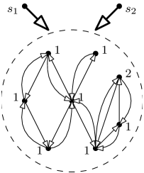
(a) The digraph $D$ obtained from the graph $G$ shown in Figure 1(a). Vertices $s_{1}$ and $s_{2}$ dominates all vertices in the dashed circle. The numbers on the vertices are the weights.

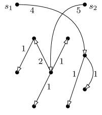
(b) A feasible solution: the arcs represent non-zero $y$-variables, and the flow in each of them is indicated on their side. Compare with the solution shown in Figure 1.

Figure 2: Digraph $D$ and a feasible solution for formulation $\mathcal{F}_{2}$.

Since each non-source vertex receives flow from at most one vertex, the flows sent by any two distinct sources do not pass through a same vertex. That is, if a source $s_{i}$ sends an amount of flow, say $w_{i}$, this amount $w_{i}$ is distributed to a subset of vertices, say $V_{i}$ (with total weight $w_{i}$); and all subsets $V_{i}$ are mutually disjoint. Moreover, $w_{i}$ is exactly the sum of the weights of the vertices that receive flow from $s_{i}$, and $G[V_{i}]$ is a connected subgraph of $G$. (See Figure 2.) It follows from these remarks that formulation $\mathcal{F}_{k}$ correctly models $\textsc{BCP}_{k}$.

The proposed formulation $\mathcal{F}_{k}(G,w)$ has a total of $2nk+4m$ variables (half of them binary), and only $\mathcal{O}(n+m+k)$ constraints, where $n:=|V(G)|$ and $m:=|E(G)|$. The possible drawbacks of this formulation are the large amount of symmetric solutions and the dependency of inequalities (9) on the weights assigned to the vertices. To overcome such disadvantages, we propose in the next section another model based on flows that considers a total order of the vertices to avoid symmetries and uncouple the weights assigned to the vertices from the flow circulating in the digraph.

4.1 A second flow formulation

Our second formulation for $\textsc{BCP}_{k}$, denoted by $\mathcal{F}^{\prime}_{k}(G,w)$, is also based on a digraph $D$ that is constructed from $G$ as follows. It has vertex set $V(D)=V(G)\cup\{s\}$ and arc set $A(D)=\{(u,v),(v,u)\colon\{u,v\}\in E(G)\}\cup\{(s,v)\colon v\in V(D)\}.$

Moreover, it assumes that there is a total ordering $\succ$ defined on the vertices of $G$. For simplicity, for a vertex $v\in V(D)\setminus\{s\}$ and integer $i\in[k]$, we use the short notation $y(\delta^{-}(v),i)$ instead of $\sum_{a\in\delta^{-}(v)}y_{a,i}$.

$$\max\> \sum_{v\in V(D)}w(v)\>y(\delta^{-}(v),1)$$

s.t. $$\sum_{v\in V(D)\setminus\{s\}}w(v)\>y(\delta^{-}(v),i)\leq\sum_{v\in V(D)\setminus\{s\}}w(v)\>y(\delta^{-}(v),i+1)\!\!\!\!\!\!\!\!\!\!\!\!\!\!\!\!\!\!\!\!\!\!\!\!\!\!\!\!\!\!\!\!\!\!\!\!\!\!\!\!\!\!\!\! \forall i\in[k-1],$$ (14)

$$\sum_{a\in\delta^{+}(s)}y_{a,i}\leq 1 \forall i\in[k],$$ (15)

$$\sum_{i\in[k]}y(\delta^{-}(v),i)\leq 1 \forall v\in V(D)\setminus\{s\},$$ (16)

$$y_{sv,i}+y(\delta^{-}(u),i)\leq 1 \forall u,v\in V(D)\setminus\{s\},v\succ u,i\in[k],$$ (17)

$$f_{a,i}\leq n\>y_{a,i} \forall a\in A(D),i\in[k],$$ (18)

$$\sum_{a\in\delta^{+}(v)}f_{a,i}\leq\sum_{a\in\delta^{-}(v)}f_{a,i} \forall v\in V(D)\setminus\{s\},i\in[k],$$ (19)

$$\sum_{i\in[k]}\sum_{a\in\delta^{-}(v)}f_{a,i}-\sum_{i\in[k]}\sum_{a\in\delta^{+}(v)}f_{a,i}=1 \forall v\in V(D)\setminus\{s\},$$ (20)

$$y_{a,i}\in\mathbb{B} \forall a\in A(D),i\in[k],$$ (21)

$$f_{a,i}\in\mathbb{R}_{\geq} \forall a\in A(D),i\in[k].$$ (22)

To show that the above formulation indeed models $\textsc{BCP}_{k}$, let us consider the following polytope:

$$\mathcal{Q}_{k}(G,w)=\operatorname{\rm{convex-hull}}\{(y,f)\in\mathbb{B}^{(n+2m)k}\times\mathbb{R}^{(n+2m)k}\colon(y,f)\text{ satisfies ineq. }\eqref{flow:ineq:asym}-\eqref{flow:ineq:real}\}.$$

Let $\mathcal{V}$ be a connected $k$-subpartition of $G$ such that $w(V_{i})\leq w(V_{i+1})$ for all $i\in[k-1]$. Then, for each integer $i\in[k]$, there exists in $D$ an out-arborescence $\vec{T}_{i}$ rooted at $r_{i}$ such that $V(\vec{T}_{i})=V_{i}$ and $v\succ r_{i}$ for all $v\in V_{i}\setminus\{r_{i}\}$. Now, let $g_{i}$ be the function $g_{i}\colon A(\vec{T}_{i})\cup\{(s,r_{i})\}\to\mathbb{R}_{\geq}$ defined as follows: $g_{i}((u,v))=1$ if $v$ is a leaf of $\vec{T}_{i}$, and $g_{i}((u,v))=1+\sum_{(v,z)\in A(\vec{T}_{i})}g_{i}((v,z))$, otherwise. It follows from this definition that $g_{i}((s,r_{i}))=|V_{i}|$.

We now define vectors $\rho(\mathcal{V})\in\mathbb{B}^{(n+2m)k}$ and $\tau(\mathcal{V})\in\mathbb{R}^{(n+2m)k}$ such that, for every arc $a\in A(D)$ and $i\in[k]$, we have

$$\rho(\mathcal{V})_{a,i}=\left\{\begin{array}[]{lr}1,&\text{ if }a\in A(\vec{T}_{i})\cup\{(s,r_{i})\}\\ 0,&\text{ otherwise,}\end{array}\right.$$

$$\tau(\mathcal{V})_{a,i}=\left\{\begin{array}[]{lr}g_{i}(a),&\text{ if }a\in A(\vec{T}_{i})\cup\{(s,r_{i})\}\\ 0,&\text{ otherwise.}\end{array}\right.$$

We are now ready to prove the claimed statement on $\mathcal{Q}_{k}(G,w)$,

Proposition 8.

The polytope $\mathcal{Q}_{k}(G,w)$ is precisely the polytope

$$\operatorname{\rm{convex-hull}}\{(\rho(\mathcal{V}),\tau(\mathcal{V}))\in\mathbb{B}^{(n+2m)k}\times\mathbb{R}^{(n+2m)k}\colon\mathcal{V}\text{ is a connected $k$-partition of }G\}.$$

Proof.

Let $(y,f)$ be an extreme point of $\mathcal{Q}_{k}(G,w)$; and for every $i\in[k]$, let $U_{i}=\{v\in V(G)\colon y(\delta^{-}(v),i)=1\}$. It follows from inequalities (16) that, for every vertex $v\in V(D)\setminus\{s\}$, at most one of the arcs entering it is chosen. Observe that inequalities (18) force that a flow of type $i$ can only pass through an arc of type $i$ if this arc is chosen. Hence, every vertex receives at most one type of flow from its in-neighbors. Furthermore, inequalities (19) and (20) guarantee that the flow that enters a vertex and leaves it are of the same type, and that each vertex consumes exactly one unit of such flow.

Inequalities (15) imply that all flow of a given type passes through at most one arc that has tail at the source $s$. Therefore, we have that $\{U_{i}\}_{i\in[k]}$ is a connected $k$-partition of $G$.

To prove the converse, let $\mathcal{V}=\{V_{i}\}_{i\in[k]}$ be a connected $k$-partition of $G$. We assume without loss of generality that $w(V_{i})\leq w(V_{i+1})$ for all $i\in[k-1]$. Let $(y,f)$ be a vector such that $y=\rho(\mathcal{V})$ and $f=\tau(\mathcal{V})$. For each $i\in[k]$, every vertex in $\vec{T}_{i}$ has in-degree at most one, and $r_{i}$ is the smallest vertex in $V(\vec{T}_{i})$ with respect to the order $\succ$. Thus, inequalities (16) and (17) hold for $(y,f)$. From the definition of $\rho(\mathcal{V})$, the entry of $y$ indexed by $(s,r_{i})$ and $i$ equals one, for all $i\in[k]$. Consequently, $(y,f)$ also satisfies inequalities (15). Recall that $g_{i}((s,r_{i}))=|V_{i}|$ for every $i\in[k]$. This clearly implies that inequalities (18) are satisfied by $(y,f)$.

Note that, for every $i\in[k]$, the function $g_{i}$ assigns to each arc $(u,v)\in A(\vec{T}_{i})\cup\{(s,r_{i})\}$ the value one plus the sum of the sizes of the sub-arborescences of $\vec{T}_{i}$ rooted at the out-neighbors of $v$ in $\vec{T}_{i}$. Hence, inequalities (19) and (20) hold for $(y,f)$. Finally, inequalities (14) are satisfied, as we assumed that the elements of partition $\mathcal{V}$ are in a non-decreasing order of weights. Therefore, we conclude that $(y,f)$ belongs to $\mathcal{Q}_{k}(G,w)$. ∎

5 Computational experiments

5.1 Benchmark instances

In order to compare the performance of our algorithms with the exact algorithms that have been proposed in the literature [18, 22], we ran our experiments on grid graphs and random connected graphs. Our algorithms are based on the three formulations that we have described in the previous sections.

The grid instances have names in the format gg_height_width_[a|b], while random connected graphs instances have names in the format rnd_n_m_[a|b], where $n$ (resp. $m$) is the number of vertices (resp. edges) of the graph. The characters (“a” or “b”) in the end of the name of an instance refer to the range of the weight distribution: character “a” (resp. “b”) indicate that the weights are integers uniformly distributed in the closed interval $[1,100]$ (resp. $[1,500]$).

To create a random connected graph with $n$ vertices and $m$ edges, with $m>n-1$, we first use Wilson’s algorithm [20] to generate a uniformly random spanning tree $T$ on $n$ vertices, and then add $m-n+1$ new edges from $E(K_{n})\setminus E(T)$ at random with uniform probability. Wilson’s algorithm returns a spanning tree $T$ sampled from the set $\tau_{n}$ — of all possible spanning trees of $K_{n}$ — with probability ${1}/{|\tau_{n}|}$.

5.2 Computational environment

The computational experiments were carried out on a PC with Intel(R) Core(TM) i7-4720HQ CPU @ 2.60GHz, 4 threads, 8 GB RAM and Ubuntu 18.04.2 LTS. The code was written in C++ using Gurobi 8.1 [19] and the graph library Lemon [7]. In order to evaluate strictly the performance of the described formulations, we deactivated all standard cuts used by Gurobi. Besides implementing the proposed formulations, we also implemented the Integer Linear Programming models introduced by Matic [18] and Zhou et al [22].

5.3 Computational results

The execution time limit was set to 1800 seconds. In the following tables, we show the number of explored nodes in the Branch-and-Bound tree (column “Nodes”) and the time (in seconds) to solve the corresponding instance (column “Time”). If the time limit is reached, the table entry shows a dash (-). Henceforth, when we refer to any of the formulations (or models) it should be understood that we are referring to the corresponding exact algorithms that we have implemented for them. Thus, cut-alg refers to the Branch-and-Cut algorithm based on formulation $\mathcal{C}_{k}$, and flow-alg and flow2-alg refer to the Branch-and-Bound algorithms based on formulations $\mathcal{F}_{k}$ and $\mathcal{F}^{\prime}_{k}$. For the sake of simplicity, the names of these algorithms are shortened to Cut, Flow and Flow2.

In Table 1, we show the impact of separating cross inequalities. Columns “CutF” and “Cut” refer to cut-alg with and without the cross inequalities, respectively. Columns “Conn. Cuts” and “Cross Cuts” show the number of connectivity and cross inequalities separated by the algorithm. We note that CutF was faster than Cut in most of the instances. Furthermore, grids gg_15_15_a and gg_15_15_b could only be solved by CutF.

Tables 2 and 3 indicate that the proposed algorithms substantially outperform the previous solution methods in the literature. On all grids instances, Flow had the best execution time. Furthermore, on grids with higher dimensions, the algorithms based on the formulations devised by Matic [18] and Zhou et al. [22] could not find a solution within the time limit. On the other hand, CutF and Flow were able to solve all the instances.

Considering the random graph instances, Table 3 shows that, on some instances, cut-alg is better than the flow-alg. Moreover, a reasonable amount of the instances were solved by Cut and Flow in the root node of the Branch-and-Bound tree.

Finally, Table 4 indicates that when the value of $k$ is greater than $2$, the problem becomes much harder to solve. Only Flow was able to solve gg_07_10_a for $k=3$ and $k=4$. For $k=5$ and $k=6$, none of the algorithms were able to solve the instance within the time limit.

Table 1: Computational results for $\textsc{BCP}_{2}$ on grid graphs with the amount of cuts added by the algorithms.

	Cut		CutF
Instance	Conn. Cuts	Time	Conn. Cuts	Cross Cuts	Time
2=1
gg_05_05_a	3242	0.73	577	796	0.17
gg_05_05_b	3527	0.87	1043	1347	0.34
gg_05_06_a	2696	0.47	58	576	0.11
gg_05_06_b	5629	1.45	1255	1310	0.30
gg_05_10_a	7544	1.80	10120	11436	3.70
gg_05_10_b	13192	4.53	2556	3703	0.67
gg_05_20_a	9802	3.86	46040	3976	47.57
gg_05_20_b	36455	23.09	4185	46185	85.53
gg_07_07_a	1074	2.9	5996	7538	3.18
gg_07_07_b	10246	3.12	7328	8258	2.20
gg_07_10_a	20397	8.42	14215	13767	5.82
gg_07_10_b	58657	71.57	23294	2255	19.24
gg_10_10_a	1178	4.62	23183	26620	17.08
gg_10_10_b	316601	1313.07	26738	28558	22.45
gg_15_15_a	0	-	83527	53287	121.56
gg_15_15_b	0	-	116041	73920	250.01

Table 2: Computational results for $\textsc{BCP}_{2}$ on grid graphs.

	CutF		Flow		Flow2		Matic		Zhou
Instance	Nodes	Time	Nodes	Time	Nodes	Time	Nodes	Time	Nodes	Time
2=1
gg_05_05_a	252	0.17	299	0.06	1697	0.23	299	0.23	674	0.17
gg_05_05_b	390	0.34	1815	0.12	1678	0.23	5957	0.74	1708	0.24
gg_05_06_a	71	0.11	323	0.06	541	0.15	6229	1.24	2134	0.46
gg_05_06_b	284	0.30	1843	0.13	202500	19.73	35627	7.49	1979	0.39
gg_05_10_a	747	3.70	343	0.10	1931	1.30	74004	14.10	7240	2.84
gg_05_10_b	300	0.67	511	0.13	1002	0.83	213650	43.46	19342	5.35
gg_05_20_a	1403	47.57	328	0.16	2825	4.69	-	-	729662	218.24
gg_05_20_b	2530	85.53	1700	0.71	396	1.07	-	-	-	-
gg_07_07_a	959	3.18	311	0.11	411	0.58	103416	16.29	14807	4.73
gg_07_07_b	615	2.20	1515	0.24	1033	1.18	483949	101.43	3255	1.43
gg_07_10_a	779	5.82	449	0.19	391	0.74	-	-	11951	6.76
gg_07_10_b	1479	19.24	606	0.16	872	1.48	-	-	18059	6.85
gg_10_10_a	1111	17.08	313	0.18	262	1.11	-	-	-	-
gg_10_10_b	1206	22.45	836	0.31	765832	595.67	-	-	3574970	957.98
gg_15_15_a	1136	121.56	155	0.40	531	6.91	-	-	-	-
gg_15_15_b	2562	250.01	1457	1.60	-	-	-	-	-	-

Table 3: Computational results for $\textsc{BCP}_{2}$ on random graphs.

	Cut		Flow		Flow2		Matic		Zhou
Instance	Nodes	Time	Nodes	Time	Nodes	Time	Nodes	Time	Nodes	Time
2=1
rnd_20_30_a	7	0.02	463	0.05	1509	0.16	6410	0.52	163	0.08
rnd_20_30_b	7	0.02	1729	0.10	7596	0.66	7249	0.91	939	0.11
rnd_20_50_a	45	0.02	323	0.06	279	0.22	117	0.12	79	0.11
rnd_20_50_b	639	0.13	311	0.07	299	0.11	1758	0.27	103	0.23
rnd_20_100_a	1	0.01	1	0.02	169	0.19	79	0.08	77	0.20
rnd_20_100_b	19	0.01	661	0.14	515	0.31	37	0.11	5	0.22
rnd_30_50_a	182	0.12	23	0.04	574	0.15	2793	0.61	594	0.19
rnd_30_50_b	55	0.08	5499	0.44	997	0.28	3169	0.62	1051	0.22
rnd_30_70_a	1	0.02	1	0.03	295	0.19	1608	0.38	203	0.37
rnd_30_70_b	15	0.03	1326	0.15	355	0.21	2721	0.84	528	0.34
rnd_30_200_a	1	0.01	1	0.06	49	0.34	1	0.11	19	0.46
rnd_30_200_b	1	0.01	57	0.17	327	0.99	2133	1.88	141	0.48
rnd_50_70_a	75	0.16	23	0.06	1026	0.41	3812	1.42	1270	0.40
rnd_50_70_b	474	0.67	787	0.10	2606	0.59	2530	1.05	1605	0.61
rnd_50_100_a	83	0.17	327	0.09	462	0.76	7548	1.78	180	0.37
rnd_50_100_b	147	0.21	15	0.05	468	0.64	5043	1.62	708	0.51
rnd_50_400_a	1	0.03	1	0.13	1	0.37	2525	2.91	99	1.47
rnd_50_400_b	1	0.03	1	0.09	478	3.22	2795	2.73	41	2.21
rnd_70_100_a	55	0.22	583	0.11	865	0.60	401	0.12	915	0.68
rnd_70_100_b	755	1.28	1112	0.19	1084	0.60	5173	2.12	1696	1.03
rnd_70_200_a	1	0.05	71	0.18	1	0.43	2235	1.15	385	1.53
rnd_70_200_b	21	0.09	1034	0.26	42	0.62	9756	2.26	267	0.62
rnd_70_600_a	1	0.01	1	0.15	35	2.05	57	0.37	1	0.70
rnd_70_600_b	19	0.07	685	0.54	1	0.80	-	-	146	3.01
rnd_100_150_a	235	2.27	71	0.15	1718	2.89	-	-	1149	1.24
rnd_100_150_b	63	0.41	539	0.19	527	1.16	1534	1.40	842	1.20
rnd_100_300_a	1	0.06	1	0.13	1381	4.89	28994	6.17	490	1.56
rnd_100_300_b	19	0.10	252	0.20	1	1.21	28837	10.39	343	2.62
rnd_100_800_a	1	0.04	1	0.24	1	1.51	105575	112.73	1	1.52
rnd_100_800_b	1	0.05	35	0.49	1	1.80	-	-	420	5.28
rnd_200_300_a	353	12.05	1	0.20	245114	147.72	358170	445.98	1917	18.27
rnd_200_300_b	1618	29.48	879	0.46	2765	12.60	49330	67.92	4606	9.69
rnd_200_600_a	1	0.12	1	0.27	2965	20.61	-	-	735	15.08
rnd_200_600_b	39	1.14	1295	0.93	5169	31.24	-	-	939	10.25
rnd_200_1500_a	1	0.08	1	0.60	1	4.67	24900	83.52	1	3.25
rnd_200_1500_b	1	0.08	1	0.51	7956	160.97	32658	103.12	489	17.31
rnd_300_500_a	227	4.88	675	0.79	4955	30.65	5848	12.15	-	-
rnd_300_500_b	827	19.65	201	0.48	3165	29.86	6917	14.28	1635	33.06
rnd_300_1000_a	1	0.23	1726	1.69	3580	48.44	7936	26.08	316	16.01
rnd_300_1000_b	1	0.55	1353	2.03	4633	61.26	-	-	642	16.74
rnd_300_2000_a	1	0.10	1	0.85	4404	132.81	12852	87.30	34	58.24
rnd_300_2000_b	1	0.16	86	1.51	2541	69.61	-	-	41	31.19

Table 4: Computational results for $\textsc{BCP}_{k}$ on a grid with height 7 and width 10.

		CutF		Flow		Flow2		Zhou
Instance	$k$	Nodes	Time	Nodes	Time	Nodes	Time	Nodes	Time
2=1
gg_07_10_a	3	-	-	1010	0.29	-	-	-	-
gg_07_10_a	4	-	-	650619	82.32	-	-	-	-
gg_07_10_a	5	-	-	-	-	-	-	-	-
gg_07_10_a	6	-	-	-	-	-	-	-	-

6 Conclusion

We proposed three mixed integer linear programming formulations for the Balanced Connected $k$-Partition Problem. To avoid some symmetries, our formulations impose an ordering of the classes $\{V_{i}\}_{i\in[k]}$, such that $w(V_{i})\leq w(V_{i+1})$, for all $i\in[k-1]$. The first one, $\mathcal{C}_{k}$, is defined on the input graph (differently from the other two formulations) and has a potentially large (i.e. exponential) number of connectivity inequalities. Moreover, we also presented a new class of valid inequalities for this formulation, and separate them on planar graphs. Computational experiments indicated that the addition of these inequalities improves greatly the performance of the algorithm. In the case the vertices have the same weight, we proved that the associated polytope is full-dimensional and characterized several inequalities that define facets of this polytope.

We also proposed two formulations based on flows in a digraph. Formulation $\mathcal{F}_{k}$ has a polynomial number of variables and constraints. To avoid symmetrical solutions and dependency on the weights of the vertices, we designed formulation $\mathcal{F}^{\prime}_{k}$. However, in our computational experiments, the performance of flow-alg was always superior to flow2-alg.

Preliminary experiments showed that both cut-alg and flow-alg have better performance when compared with the exact algorithms in the literature. We plan to carry out further experiments on more instances, specially on some real data (e.g. problems on police patrolling), to evaluate the performance of all algorithms mentioned in this work.

References

- [1] P. Alimonti and T. Calamoneri. On the complexity of the max balance problem. In Argentinian Workshop on Theoretical Computer Science (WAIT’99), pages 133–138, 1999.
- [2] R. I. Becker and Y. Perl. Shifting algorithms for tree partitioning with general weighting functions. Journal of Algorithms, 4(2):101–120, 1983.
- [3] R. Borndörfer, Z. Elijazyfer, and S. Schwartz. Approximating balanced graph partitions. Technical Report 19-25, ZIB, Takustr. 7, 14195 Berlin, 2019.
- [4] F. Chataigner, L. R. B. Salgado, and Y. Wakabayashi. Approximation and inapproximability results on balanced connected partitions of graphs. Discrete Mathematics & Theoretical Computer Science, Vol. 9 no. 1, 2007.
- [5] J. Chlebíková. Approximating the maximally balanced connected partition problem in graphs. Information Processing Letters, 60(5):225–230, 1996.
- [6] M. P. de Aragão and E. Uchoa. The -connected assignment problem. European Journal of Operational Research, 118(1):127–138, 1999.
- [7] B. Dezső, A. Jüttner, and P. Kovács. Lemon–an open source c++ graph template library. Electronic Notes in Theoretical Computer Science, 264(5):23–45, 2011.
- [8] M. Dyer and A. Frieze. On the complexity of partitioning graphs into connected subgraphs. Discrete Applied Mathematics, 10(2):139–153, 1985.
- [9] J. Edmonds. Paths, trees, and flowers. Canadian Journal of mathematics, 17:449–467, 1965.
- [10] G. Galbiati, A. Morzenti, and F. Maffioli. On the approximability of some maximum spanning tree problems, pages 300–310. Springer Berlin Heidelberg, Berlin, Heidelberg, 1995.
- [11] G. Galbiati, A. Morzenti, and F. Maffioli. On the approximability of some maximum spanning tree problems. Theoretical Computer Science, 181(1):107–118, 1997.
- [12] M. Grötschel, L. Lovász, and A. Schrijver. Geometric algorithms and combinatorial optimization, volume 2. Springer Science & Business Media, 2012.
- [13] K. Kawarabayashi, Y. Kobayashi, and B. Reed. The disjoint paths problem in quadratic time. Journal of Combinatorial Theory, Series B, 102(2):424–435, 2012.
- [14] M. Lucertini, Y. Perl, and B. Simeone. Image enhancement by path partitioning, pages 12–22. 1989.
- [15] M. Lucertini, Y. Perl, and B. Simeone. Most uniform path partitioning and its use in image processing. Discrete Applied Mathematics, 42(2):227–256, 1993.
- [16] M. Maravalle, B. Simeone, and R. Naldini. Clustering on trees. Computational Statistics & Data Analysis, 24(2):217–234, 1997.
- [17] D. Matić and M. Božić. Maximally balanced connected partition problem in graphs: application in education. The Teaching of Mathematics, (29):121–132, 2012.
- [18] D. Matić. A mixed integer linear programming model and variable neighborhood search for maximally balanced connected partition problem. Applied Mathematics and Computation, 237:85–97, 2014.
- [19] G. Optimization. Inc.,“Gurobi optimizer reference manual,” 2015. URL: http://www. gurobi. com, 2014.
- [20] D. B. Wilson. Generating random spanning trees more quickly than the cover time. In STOC, volume 96, pages 296–303. Citeseer, 1996.
- [21] B. Y. Wu. Fully polynomial-time approximation schemes for the max-min connected partition problem on interval graphs. Discrete Mathematics, Algorithms and Applications, 04(01):1250005, 2012.
- [22] X. Zhou, H. Wang, B. Ding, T. Hu, and S. Shang. Balanced connected task allocations for multi-robot systems: An exact flow-based integer program and an approximate tree-based genetic algorithm. Expert Systems with Applications, 116:10–20, 2019.