Deep learning velocity signals allows to quantify turbulence intensity

Abstract

Turbulence, the ubiquitous and chaotic state of fluid motions, is characterized by strong and statistically non-trivial fluctuations of the velocity field, over a wide range of length- and time-scales, and it can be quantitatively described only in terms of statistical averages. Strong non-stationarities hinder the possibility to achieve statistical convergence, making it impossible to define the turbulence intensity and, in particular, its basic dimensionless estimator, the Reynolds number.

Here we show that by employing Deep Neural Networks (DNN) we can accurately estimate the Reynolds number within $15\%$ accuracy, from a statistical sample as small as two large-scale eddy-turnover times. In contrast, physics-based statistical estimators are limited by the rate of convergence of the central limit theorem, and provide, for the same statistical sample, an error at least $100$ times larger. Our findings open up new perspectives in the possibility to quantitatively define and, therefore, study highly non-stationary turbulent flows as ordinarily found in nature as well as in industrial processes.

Turbulence is characterized by complex statistics of velocity fluctuations correlated over a wide range of temporal- and spatial-scales. These range from the integral scale, $L$, characteristic of the energy injection (with correlation time $T_{L}$), to the dissipative scale, $\eta\ll L$, characteristic of the energy dissipation due to viscosity (with correlation time $\tau_{\eta}\ll T_{L}$). The intensity of turbulence directly correlates with the width of this range of scales, $L/\eta$ or $T_{L}/\tau_{\eta}$, commonly dubbed inertial range.

In statistically stationary, homogeneous and isotropic turbulence (HIT), the width of the inertial range, is well known to correlate with the Reynolds number, $Re$, defined as $Re=v_{rms}L/\nu$, where $v_{rms}$ is the characteristic velocity fluctuation at the integral scale, and $\nu$ is the kinematic viscosity. Therefore the value of the Reynolds number is customarily used to quantify turbulence intensity. While this value remains well-defined in laboratory experiments, performed under stationary conditions, and for fixed flow configurations ($L=const$), its quantification results impossible when we consider turbulence in open environments (as in many outstanding geophysical situations) or in non-stationary situations (such as turbulent/non-turbulent interfaces). This observation is linked to the question: can we estimate turbulence intensity from fluctuating velocity signals of arbitrary (short) length? For statistically stationary conditions, this is indeed possible provided enough statistical samples are available and by using appropriate physics-based statistical averages of the fluctuating velocity field. For non-stationary turbulent flows (i.e. changing on timescales comparable with the large-scale correlation times) the question itself appears meaningless. In these conditions, the intertwined complexity of a slow large-scale dynamics and of fast, but highly intermittent, small-scale fluctuations, makes impossible to estimate reliably the width of the inertial range.

In this paper we demonstrate, using a proof of concept, that our fundamental question can be answered by a suitable use of machine learning. We propose a machine learning Deep Neural Network (DNN) model capable of estimating turbulence intensity within $15\%$ accuracy from short velocity signals (duration $T$: approximately two large-scale eddy turnover times, i.e. $T\approx 2\,T_{L}$, where $T_{L}\approx L/v_{rms}$). We remark that analyzing the same data via standard statistical observables of turbulence leads to quantitatively meaningless results (predictions between $10^{-2}$ and $10^{2}$ times the true value).

We train the DNN model to predict turbulence intensity using (short) Lagrangian velocity signals obtained from HIT. As Lagrangian velocities are one of the most intermittent features of turbulence, we are choosing the most difficult case for our proof of concept. The Lagrangian velocity signals, $v(t)$, that we employ are obtained as the superposition of different strongly chaotic time signals, $u_{n}(t)$, derived from a shell model of turbulence [4, 9] (see Methods). The velocity signals, $v(t)$, are known to match the statistical properties of the velocity experienced by a passive Lagrangian particle in HIT [5]. The shell model describes the nonlinear energy transfer among different spatial scales, $l_{n}=1/k_{n}$, where $k_{n}=L^{-1}\lambda^{n}$ (with $L^{-1}=0.05$ being the wave number associated with the integral scale, and $\lambda=2$ defining the ratio between successive shells). The nonlinear energy transfer is characterized by sudden bursts of activity (typically referred to as “instantons”) [4, 7], where anomalous fluctuations are spread from large- to small-scales. The complex space-time patterns and localized correlations in $v(t)$, given by these intermittent bursts, make a 1-dimensional Convolutional Neural Network a well-suited choice for our neural network model (see Methods and SI for details).

We train the DNN using a collection of datasets corresponding to different viscosity values for our Lagrangian turbulent signal. Each dataset includes a large number of velocity signals (few thousands) sampled over $2048$ time instants (see examples in Figure 1(a)). We decided to employ an external forcing to maintain the root-mean-square energy fluctuations of the signals, and thus $v_{rms}$, statistically stationary. As a result, the viscosity fully determined the turbulence intensity, and therefore the Reynolds number. Decreasing the viscosity increases the high-frequency content of the velocity signals (as $\sim Re^{1/2}$, cf. time-increments in Figure 1(b)) by reducing the dissipative time- and length-scales. The resulting wider inertial range reflects the higher turbulence intensity. We train the network in a supervised way to infer the viscosity from the velocity signals; the collection of datasets covered uniformly the viscosity interval $10^{-5}\leq\nu\leq 10^{-3}$ in $39$ equi-spaced levels.

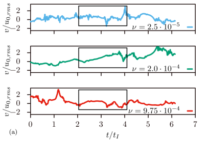
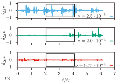
Figure 1: Velocity signals, $v(t)$, used to train the DNN for three different values of the viscosity $\nu$. The signals are normalized with the rms of the integral-scale velocity, $u_{0,rms}\approx v_{rms}$. The time is reported in units of eddy turnover times of the integral scale, $T_{L}$ ($T_{L}\approx 1000\Delta t$, being $\Delta t$ the time sampling of the signals input to the DNN). Each training signal spans $2048$ samples, i.e. about two eddy turnover times (the rectangular frames identify individual training signals). (b) Velocity increments, $\delta_{\Delta t}v(t)=v(t+\Delta t)-v(t)$, computed with time interval $\Delta t$. Lower viscosity values yield higher turbulence intensity, thus more intermittent high-frequency components and more intense small-scale velocity differences.

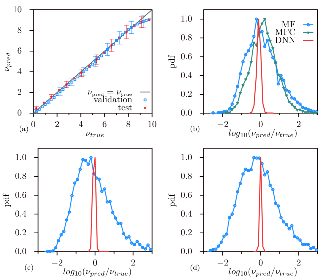
Figure 2: (a) Average predictions of viscosity, $\nu$, by the DNN ($\nu_{pred}$, $y$-axis) vs. ground truth ($\nu_{true}$, $x$-axis), for the validation and test sets considered (the axes are scaled by a factor $10^{-4}$). The diagonal line identifies error-free predictions, i.e. $\nu_{pred}=\nu_{true}$. We include a few indicative error bars of size $\pm\sigma$ from the average, to indicate the typical spread of the prediction. (b,c,d) Comparison of the viscosity estimates over three viscosity levels in the validation set, respectively, $\nu=0.000075$, $0.0002$ and $0.0007$). We report the pdf of $\log_{10}(\nu_{pred}/\nu_{true})$ for the DNN (solid line), and for the multifractal model (dotted-line), Eq. (1). Evaluating $v_{rms}$ in Eq. (1) through an ensemble averaged (MF), or individually for each signal as $v_{rms}=\frac{1}{2}S^{2}(\infty)\approx\frac{1}{2}S^{2}(T)$ (MFC), yields similar results, which we report panel (b). We notice how the predictions based on Eq. (1), once normalized to the true value, range within about four orders of magnitude, whereas they remain confined within $15\%$ accuracy in the case of the DNN.

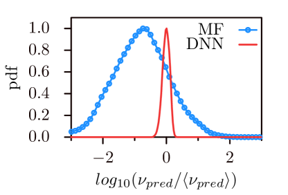
Figure 3: Comparison of the viscosity estimates by the DNN (trained through shell model data, solid line), and by the multifractal model (MF, dotted-line) for Lagrangian velocity signals obtained by a DNS simulation. We normalize the estimates by the most frequent prediction, $\langle\nu_{pred}\rangle$, i.e. we report the pdf of $\log_{10}(\nu_{pred}/\langle\nu_{pred}\rangle)$. This enables a comparison of the prediction root-mean-squared errors. As in the considered validation and test cases, the DNN estimates fall within a significantly smaller range than in case of predictions by the multifractal model. Note that a log-normal distribution is expected for the viscosity estimates [3], thus the discrepancy between average and most frequent prediction, clearly evident in the MF case.

We assess the predictive performance of the DNN by considering unseen signals generated by the shell model. Results are reported in Figure 2 where two different test sets are used: 1) “validation set”: including statistically independent realizations of the velocity signals than the training phase, yet having the same viscosity values; 2) “test set”: signals having different viscosity values than considered during training, yet within the same viscosity range. The results demonstrate that the network is capable of very accurate predictions for the viscosity over the full range considered, also for viscosity values different from those employed in training. By aggregating the viscosity estimates over a large number of statistically independent shell model signals with fixed viscosity, we can define an average estimate as well as a root-mean-squared error, see Figure 2(a).

To further reflect on this remarkable result, we turn to a physical argument for estimating the viscosity. For the second-order Lagrangian structure functions $S^{2}(\tau)=\langle\delta_{\tau}v(t)^{2}\rangle$, where $\delta_{\tau}v(t)=v(t+\tau)-v(t)$, in steady HIT the following estimate holds in the small $\tau$ limit:

$$S^{2}(\tau)=Av_{rms}^{2}\left(\frac{\tau}{T_{L}}\right)^{2}Re^{\alpha},$$ (1)

where $A$ is a constant of order $1$, $\alpha=0.57$, and $v_{rms}^{2}/T_{L}\equiv\epsilon$ is the Reynolds-independent rate of energy dissipation [1]. The (dissipative) time-scale $\tau_{\eta}$ is defined by the relation $S^{2}(\tau_{\eta})/\tau_{\eta}=\epsilon$ which, using Eq. (1), gives $\tau_{\eta}/T_{L}=Re^{-\alpha}/A$. Assuming $L$ and $v_{rms}$ known, or, alternatively estimating $v_{rms}^{2}=1/2S^{2}(\infty)\approx 1/2S^{2}(2\,T_{L})$ on a signal-by-signal basis, to amend for large-scale oscillations within the observation window, we evaluate $A$ by using a reference case of known viscosity, say $\nu_{0}$. Figure 2(b,c,d) compare the pdfs of the logarithmic ratio between the estimated and true viscosity, for estimates by the DNN and based on Eq. (1). Predictions in case of Eq. (1) spread over a range $\nu_{pred}/\nu_{true}\in[10^{-2},10^{2}]$, whereas this range is just of order $15\%$ in case of the DNN. Besides, in Figure 2(b), we observe that evaluating $v_{rms}$ on a signal-by-signal basis reduces, yet minimally, the variance of viscosity predictions based on Eq. (1).

The high variance and heavy tails of the pdf of viscosity estimates produced by Eq. (1) follow from the very limited statistical sampling ($2048$ points), which is severely affected by large-scale oscillations and small-scale intermittent fluctuations. Because of these, statistical convergence and, therefore, a stable value for the LHS of Eq. (1), are attained only after very long observation times.

Our DNN model can be tested on real Lagrangian velocity signals, $v(t)$, obtained by the numerical integration of the Lagrangian dynamics of a tracer particle in HIT, see Figure 3. The underlying Eulerian velocity field is obtained from Direct Numerical Simulation [2] of the Navier-Stokes equation at $Re_{\lambda}=400$ (see Methods). Remarkably, the DNN, although trained on shell model data, is able to estimate with extremely high accuracy the viscosity $\nu$ even in case of real Lagrangian data (note that Lagrangian velocity signals from DNS has been exhaustively validated against experimental data in the past [11]). This points to the fact that the DNN relies on space-time features that are equally present in the shell model as well as in the real Lagrangian signals.

What is the best result that can be achieved according to the current understanding of the physics of turbulence? Both by direct estimation of the Reynolds number or by viscous scale fitting, i.e. using Eq. (1), the statistical accuracy is limited by the fluctuations of the large-scale velocity. Therefore, the statistical error is limited by the number of large-scale eddy turnover times. As shown in Figure 2(b,c,d), a traditional statistical physics approach produces estimates for the viscosity spread over four orders of magnitude, while the DNN is capable of delivering accurate predictions, scattering within a $15\%$ range.

This points at two major results: first, the DNN, at least within the range of the training signals, must be able to identify space-time structures that strongly correlate with turbulence intensity and which are rather insensitive to the strong fluctuations of the instantaneous value of the large-scale velocity (cf. SI for a discussion). This finding unlocks the possibility of defining, practically instantaneously, turbulence intensities, Reynolds numbers, or connected statistical quantities for complex flows and fluids. Estimating locally, in space and in time, the turbulence intensity at laminar-turbulent interfaces or from atmospheric anemometric readings can now be possible. The quantitative definition of an effective viscosity within boundary layers or complex fluids, such as emulsions or viscoelastic flows, may similarly be pursued. Finally, being able to extract the space-time correlations identified by the DNN may give us novel and fundamental insights in turbulence physics and the complex skeleton of the fluctuating turbulent energy cascades.

Methods

Generating the database of turbulent velocity signals

We employ the SABRA [9] shell model of turbulence to generate Lagrangian velocity signals $v(t)=\sum_{n\geq 0}\Re{u_{n}(t)}$ corresponding to different turbulence levels (Reynolds numbers). Shell models evolve in time, $t>0$, the complex amplitude of velocity fluctuations, $u_{n}(t)$, at logarithmically spaced wavelengths, $k_{n}=k_{0}\lambda^{n}$ ($n=0,1,\ldots$).

The amplitudes $u_{n}(t)$ evolve according to the following equation:

$$\frac{du_{n}(t)}{dt}=i(ak_{n+1}u_{n+2}u^{*}_{n+1}+bk_{n}u_{n+1}u^{*}_{n-1}-ck_{n-1}u_{n-1}u_{n-2})-\nu k_{n}^{2}+f_{n}(t),$$ (2)

where $\nu>0$ represents the viscosity, $f_{n}(t)$ is the forcing, and the real coefficients $a,b,c$ regulate the energy exchange between neighboring shells. We consider the following constraints: $a+b+c=0$, which guarantees conservation of energy $E=\sum_{n}|u_{n}|^{2}$, for an unforced and inviscid system ($f_{n}=0$, $\nu=0$, respectively); $b=-1/2$, which gives to the second (inviscid/unforced) quadratic invariant of the system, $H=\sum_{n\geq 0}(-)^{n}k_{n}|u_{n}|^{2}$, the dimensions of an helicity; to fix the third parameter we opt for the common choice $c=1/2$. We truncate Eq. (2) to a finite number of shells $0\leq n<\ N=28$ which ensures a full resolution of the dissipative scales in combination with our forcing and viscosity range. We simulate the system in Eq. (2) via a $4^{th}$ Runge-Kutta scheme with viscosity explicitly integrated [6] (the integration step, $dt$, is fixed for all simulations, to be about three orders of magnitude smaller than the dissipative time-scale for the lowest viscosity case).

We inject energy through a large-scale forcing acting on the first two shells [9]. The forcing dynamics is given by an Ornstein-Uhlenbeck process with a timescale matching the eddy turnover of the forced shells ($\tau_{n}=(k_{n}u_{n})$, $n=0,1$). Additionally, we set the ratio $|\sigma(f_{0})/\sigma(f_{1})|=\sqrt{2}$ between the standard deviation ($\sigma(f_{n})$) of the two forcing signals. This ensures a helicity-free energy flux in the system [9]. See the SI for further information on the signals and values of the constants.

We generate the signals in a vectorized fashion on an nVidia V100 card. We integrate simultaneously $15.000$ instances of the system in Eq. (2) in a vectorized manner (i.e. system description by $15.000\times 28$ complex variables), and dump the state $55.000$ times after skipping the first $5.000$ samples.

Lagrangian velocity signals from Direct Numerical Simulations

The true Lagrangian velocity signals are obtained from the numerical integration of Lagrangian tracers dynamics evolved on top of a Direct Numerical Simulation of HIT turbulence. The Eulerian flowfield is evolved via a fully de-aliased algorithm with second-order Adams-Bashfort time-stepping with viscosity explicitly integrated. The Lagrangian dynamics is obtained via a tri-linear interpolation of the Eulerian velocity field coupled with second-order Adams-Bashfort integration in time. The Eulerian simulation has a resolution of $2048^{3}$ grid points, a viscosity of $3.5\cdot 10^{-4}$, a timestep $dt=1.2\cdot 10^{-4}$, this corresponded to a $Re_{\lambda}~{}400$, dissipative scale $\eta=3\cdot 10^{-3}$ and $\tau_{\eta}=2\cdot 10^{-2}$. The Lagrangian trajectories employed are available at the 4TU.Centre for Research Data [8].

Deep Neural Network (DNN)

We employ a one-dimensional Convolutional Neural Network (CNN) architecturally inspired by the VGG model [10]. Developing a neural network model poses the major challenge of selecting a large number of hyperparameters. This particular architecture deals with this issue by fixing the size of the filters and employs stacks of convolutional layers to achieve complex detectors. For our model we opted for convolutional filters of size $3$, which is comparable or smaller than the dissipative time-scale of the turbulent signals. The network includes four blocks, each formed by three convolutional layers (including $128$ filters each), a max pooling layer (window: 2) and a dropout layer, that capture all the spatial features of the signal (cf. DNN architecture in SI). These layers are followed by a fully-connected layer with $128$ neurons and Re-Lu activation that collects all the spatial features into a dense representation. The final layer provides a linear map from the dense representation to the estimated viscosity. A complete sketch of the network is in the SI.

DNN Training

We train the neural network in a supervised fashion and with $L^{2}$ training loss to output a continuous value in the interval $[-1,1]$, which is linearly mapped to $[\min\nu,\max\nu]$. The training set is composed of $192.000$ turbulent velocity signals (time-sampled over $2048$ points) uniformly distributed among $39$ viscosity levels (training-validation ratio: 75%-25%). See Table in SI for further information.

Supplementary Information (SI)

Width of the inertial range

In presence of limited statistics as in the case of relatively short signals, the estimation of the width of the inertial range or, similarly, the estimation of the viscosity, is enslaved to large scale energy fluctuations. On a time scale comparable to the large scale fluctuations, local increments or decrements of the system energy yield almost instantaneous widenings or shortenings of the inertial range. This effect can be naturally interpreted in terms of viscosity, where local energy increments play the same effect of a lower viscosity on the width of inertial range (see Figure S.1, where show this aspect for Eulerian structure functions).

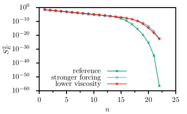
Figure S.1: Impact of the variation of forcing (operating at the large scale, $L$) or viscosity (regulating the small scale, $\eta$) on Eulerian structure functions. We compare a reference case with, respectively, a dynamics characterized by increased forcing (structure function translated and superimposed, a posteriori, to the reference), and a dynamics characterized by decreased viscosity. Both these two cases yield a higher Reynolds number wider extension of the inertial range.

In Figure S.2(a), we report Lagrangian structure functions for a set of training signals with fixed viscosity values. The limited statistics yield high fluctuations among the structure function, due to a combination of large-scale energy fluctuations and small scale intermittency. In Figure S.2(b), we amend large-scale fluctuations by normalizing by the signal energy, i.e. we report $S^{2}(\tau)/S^{2}(\infty)$.

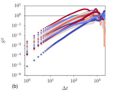
Figure S.2: Collection of second order Lagrangian structure functions, $S^{2}$, without (a) and with (b) normalization with respect to the integral scale energy, i.e. the asymptotic value $S^{2}(\infty)=2v_{rms}^{2}\approx S^{2}(T)$. Each plot reports a collection of $25$ structure functions extracted from the training set and with associated viscosity $\nu=0.0005$. The x-axis is in units of sampling time, $\Delta t$, as presented to the DNN.

Data generation, training, testing and neural network parameters

We include in Table 1 the parameters considered in the shell model simulations by which the training, validation and test datasets have been created. In Figure S.3 we complement Figure 1 by including, for the same three viscosity levels, further features of the considered signals. These are: (a) second order Eulerian structure functions, $S^{2}_{E}(n)$ (where $S^{p}_{E}(n)=S^{p}_{E}(k_{n})=\left\langle|u_{n}|^{p}\right\rangle$) showing that changing the viscosity only affects the extension of the inertial range; (b) relevant time scales (computed by inertial scaling) associated with the dynamics of the different shells; (c) signals energy as a function of time. In Figure S.4, we report the diagram of the neural network. Relevant structural parameters (e.g. size of the convolutional filters) are reported in the figure caption.

Parameter	Value
$N$	$28$	Number of shells
$k_{0}$	$0.05$	Wave number integral scale
$\lambda$	2	Inter-shell distance
$\sigma(f_{0})$	$2$	Noise intensity forcing on shell $0$
$\sigma(f_{1})$	$2/\sqrt{2}$	” on shell $1$
$dt$	$5\cdot 10^{-5}$	integration step
$\Delta t$	$1000\,dt$	sampling time DNN
$T$	$2048\,\Delta t$	length window DNN

Parameter	Training	Testing
$\min(\nu)$	$2.5\cdot 10^{-5}$	$6.0\cdot 10^{-5}$
$\max(\nu)$	$9.75\cdot 10^{-4}$	$9.6\cdot 10^{-4}$
increment $\nu$	$2.5\cdot 10^{-5}$	$6.0\cdot 10^{-5}$
levels	$39$	$16$
set size	192.000	6.600
training:validation ratio	75%:25%	N/A

Table 1: (Top) Relevant parameters for the shell model its numerical integration; time length and sampling of the signals as provided to the deep neural network (DNN). (Bottom) Viscosity values considered for training validation and test; size of the related datasets.

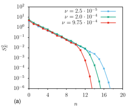
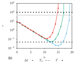
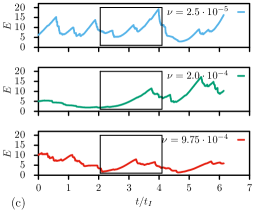
Figure S.3: (a) Eulerian structure functions $S^{2}_{E}(n)=\langle|u_{n}|^{2}\rangle$ for the same three viscosity cases reported in Figure 1. Reducing the viscosity leads to an extension of the inertial range, while the energy content of the larger scales remains unchanged. (b) A scale-by-scale estimate of the correlation times for the shell models (via the inertial scaling $\tau_{n}\sim(k_{n}u_{n,rms})^{-1}$) for three different viscosity values. The observation window $T$, the calculated decorrelation time of the integral scale $T_{L}$, and of the DNN sampling time $\Delta t$ are reported. (c) Energy time-histories for the signals reported in Figure 1.

Figure S.4: Feed-forward convolutional neural network considered. The network is constituted of four blocks each encompassing three convolutional layers (“conv”, filter size $f_{s}=3$, filter number $f_{M}=128$, activation function: Re-Lu) one max pool layer that down scales the signal by a factor two and, in training, a dropout layer with dropout probability $20\%$. The dimensions of the feature map as obtained at the end of each block is reported in the dashed rectangles. The last feature map (dimension $(128,128)$), is densely connected to a representation layer which has $f_{d}=128$ dimensions and Re-Lu activation. The final output, i.e. the predicted viscosity $\nu$, is built from a linear combination of the dense representation values.

Features observed by the DNN

During training, the DNN develops feature detectors. As discussed in the main text, we expect these detectors to select features that, at the same time, strongly correlate with the turbulence intensity and that are insensitive to large scale oscillations. As generally expected in deep learning, detectors are likely specific to the parameter range and statistical properties of the signals contained in the training set.

In this section, to understand the characteristics of the signal that our model relies on, we develop an ablation study by systematically altering the content of randomly selected testing signals. The modifications considered involve the suppression of frequency components, or the random shuffling of the time structure. This enables us to identify features mostly ignored by the DNN and, conversely, restrict the set of characteristics of the signals relevant for the DNN.

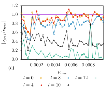
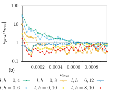
Figure S.5: Viscosity predictions with ablated input signals from (a) an highpass filter: $v(t)=Re\sum_{n=l}^{26}u_{n}(t)$, (b) a bandpass filter: $v(t)=Re\sum_{n=l}^{h}u_{n}(t)$. In both cases, one single sample signal is considered for each viscosity value. Predictions are reported normalized with respect to the true value.

In Figure S.5 we consider testing signals that have been altered through a high-pass (a) or a band-pass filter (b). In the case of Lagrangian signals, filtering operations are easily performed by restricting the summation in Eq. (2) to a subset of the shell signals. We select one testing signal per viscosity level, we ablate its spectral structure and we plot the DNN prediction. We notice that the neural network is almost insensitive to the large scale dynamics, as the estimates after the high-pass filter remain unaltered if the large-scale shells are removed. We notice, in particular, that any selection of a band of shells that includes the last part of the inertial range yield almost error-free predictions.

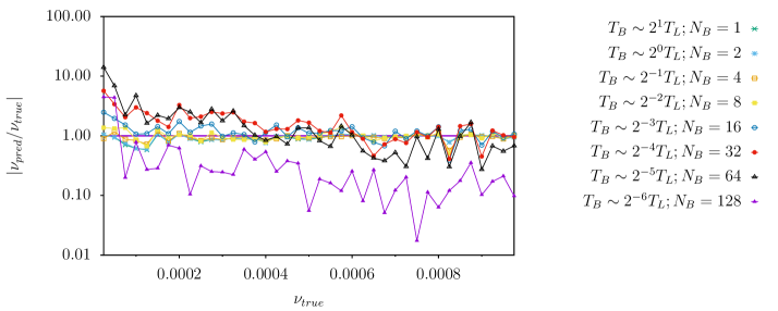
Figure S.6: Viscosity predictions for block-based time-altered signals. Alteration is performed by splitting an initial signal in $N_{B}$ blocks (with time length $T_{B}$ reported in terms of the integral time scale) and then by performing a random permutation of the blocks. One single sample signal is considered for each viscosity value. Predictions are reported normalized with the true value.

Similarly, we can alter the time structure of the signals by partitioning them in disjoint contiguous blocks of length $T_{B}$, and then by randomly mixing these blocks. In Figure S.6 we report the predictions for different block extensions. As the block extension remains in the same order of the integral scale, the prediction remain mostly unaltered, to then degrade as the block size become comparable to the dissipative time-scale. This shows how the training develop feature extractors targeting fine scales and correlations existing around the dissipative end of the inertial range.

References

- [1] A. Arnéodo, R. Benzi, J. Berg, L. Biferale, E. Bodenschatz, A. Busse, E. Calzavarini, B. Castaing, M. Cencini, L. Chevillard, et al. Universal intermittent properties of particle trajectories in highly turbulent flows. Physical Review Letters, 100(25):254504, 2008.
- [2] J. Bec, L. Biferale, M. Cencini, A. Lanotte, and F. Toschi. Intermittency in the velocity distribution of heavy particles in turbulence. Journal of Fluid Mechanics, 646:527–536, 2010.
- [3] R. Benzi, G. Paladin, G. Parisi, and A. Vulpiani. Characterisation of intermittency in chaotic systems. Journal of Physics A: Mathematical and General, 18(12):2157, 1985.
- [4] L. Biferale. Shell models of energy cascade in turbulence. Annual Review of Fluid Mechanics, 35(1):441–468, 2003.
- [5] G. Boffetta, F. De Lillo, and S. Musacchio. Lagrangian statistics and temporal intermittency in a shell model of turbulence. Physical Review E, 66(6):066307, 2002.
- [6] T. Bohr, M. H. Jensen, G. Paladin, and A. Vulpiani. Dynamical systems approach to turbulence. Cambridge University Press, 2005.
- [7] I. Daumont, T. Dombre, and J.-L. Gilson. Instanton calculus in shell models of turbulence. Physical Review E, 62(3):3592, 2000.
- [8] A. Lanotte, E. Calzavarini, F. Toschi, J. Bec, L. Biferale, and M. Cencini. Heavy particles in turbulent flows rm-2007-grad-2048. Dataset available online, 4TU.Centre for Research Data, 2011.
- [9] V. S. L’vov, E. Podivilov, A. Pomyalov, I. Procaccia, and D. Vandembroucq. Improved shell model of turbulence. Physical Review E, 58(2):1811, 1998.
- [10] K. Simonyan and A. Zisserman. Very deep convolutional networks for large-scale image recognition. 3rd International Conference on Learning Representations, arXiv:1409.1556, 2015.
- [11] F. Toschi and E. Bodenschatz. Lagrangian properties of particles in turbulence. Annual review of fluid mechanics, 41:375–404, 2009.