Towards exact solutions for the superconducting $T_{c}$ induced by electron-phonon interaction

Abstract

Electron-phonon interaction plays an important role in metals and can lead to superconductivity and other instabilities. Previous theoretical studies on superconductivity are largely based on the Migdal-Eliashberg theory, which neglects all the vertex corrections to electron-phonon coupling and breaks down in many unconventional superconductors. Here, we go beyond the Migdal-Eliashberg approximation and develop a nonperturbative Dyson-Schwinger equation approach to deal with the superconducting transition. Remarkably, we take into account all the vertex corrections by solving two coupled Ward-Takahashi identities derived from two global U(1) symmetries and rigorously prove that the fully renormalized electron propagator satisfies a self-closed integral equation that is directly amenable to numerical computations. Our approach works equally well in the weak and strong coupling regimes and provides an efficient method to determine superconducting $T_{c}$ and other quantities. As an application, our approach is used to investigate the high-$T_{c}$ superconductivity in one-unit-cell FeSe/SrTiO₃.

I Introduction

In crystalline solids, atoms are arranged in a highly ordered pattern, forming periodic lattices. Phonons, the quanta of collective vibrating modes of atoms, interact with the mobile electrons of metals. The electron-phonon interaction (EPI) plays a major role in all metals Schrieffer64 ; AGD ; Scalapino , and governs many thermodynamic and transport properties. Under proper conditions, EPI may induce a number of possible phase-transition instabilities, such as superconductivity and charge density wave (CDW). Metals cannot be thoroughly understood without detailed knowledge of EPI. Finding a reliable method to efficiently treat the EPI-induced quantum many-body effects is one of the greatest challenges in condensed-matter physics.

A remarkable consequence of EPI is the realization of superconductivity. Comparing to CDW and other phases, superconductivity is more universal, of broader interest, and also has much more technical and industrial applications. We believe that superconductivity provides an ideal framework to develop new nonperturbative quantum many-body methods. According to Bardeen-Cooper-Schrieffer (BCS) theory Schrieffer64 , a sufficiently strong EPI triggers Cooper pairing (see Fig. 1 for a schematic illustration) and then leads to superconductivity. It has been established that EPI is responsible for the onset of superconductivity in a large number of conventional Schrieffer64 ; AGD ; Scalapino ; Migdal ; Eliashberg ; Allen ; Carbotte ; Marsiglio19 and unconventional Xue12 ; Shen14 ; Lee15 ; Gorkov16 ; Johnston-NJP2016 ; Martin19 superconductors. To understand the properties of these superconductors, it is important to find a quantitatively reliable tool to accurately compute the superconducting transition temperature $T_{c}$ and other relevant quantities. Without such a tool, it would be hard to predict and apply realistic superconducting materials. While the BCS theory identifies the correct microscopic mechanism of superconductivity, it is a mean-field theory and cannot compute the accurate value of $T_{c}$ in most superconductors. The oversimplified BCS theory can be improved by the Migdal-Eliashberg (ME) theory Migdal ; Eliashberg , which incorporates the retardation of phonon propagation, electron mass renormalization, and Cooper pairing in a self-consistent manner.

In the past sixty years, the ME theory has been extensively adopted to investigate EPI-induced effects in numerous superconductors Schrieffer64 ; AGD ; Scalapino ; Allen ; Carbotte ; Marsiglio19 , and is widely regarded as the standard theory of conventional superconductivity. Specifically, it plays an overwhelmingly dominant role Allen in the computation of superconducting $T_{c}$. The reliability of ME theory depends heavily on the validity of Migdal theorem Migdal , which states that all the quantum corrections to the EPI vertex function $\Gamma_{\mathrm{v}}(q,p)$ are suppressed by the small factor $\lambda(\omega_{D}/E_{F})$, where $\lambda$ is a dimensionless coupling constant, $\omega_{D}$ is the phonon frequency, and $E_{F}$ is the Fermi energy, and therefore can be completely ignored if $\lambda(\omega_{D}/E_{F})\ll 1$. The ME results are expected to be reliable as long as the ratio $\omega_{D}/E_{F}$ is sufficiently small and/or the EPI is sufficiently weak. However, it has long been recognized that the Migdal theorem is not always valid Engelsberg63 ; Alexandrov01 ; Kivelson18 . There exist several classes of superconductors in which $\lambda(\omega_{D}/E_{F})$ is not small. Notable examples include low carrier-density superconductors such as SrTiO₃ Schooley64 ; Chubukov19 and Moiré superconductor Caoyuan18 ; Martin19 , fulleride superconductors Gunnarsson97 ; Cappelluti01 , cuprate superconductors Carbotte ; Shen05 , and one-unit-cell (1UC) FeSe/SrTiO₃ system Xue12 ; Shen14 ; Lee15 ; Gorkov16 ; Johnston-NJP2016 . The ME results become especially unreliable when EPI gets strong. This fact has already been discussed Engelsberg63 ; Alexandrov01 ; Gunnarsson97 ; Cappelluti01 for decades, and recently was re-confirmed by a determinant quantum Monte Carlo (DQMC) study Kivelson18 . To describe EPI systems in which the Migdal theorem breaks down, it is necessary to develop a more powerful approach that can take into account all the potentially important contributions omitted in the ME theory and meanwhile is valid in both the weak and strong regimes of EPI.

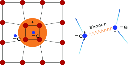
Figure 1: Schematic illustration of electron-phonon interaction. A mobile electron attracts another mobile electron by exchanging phonons. Two electrons with opposite momenta and spin directions are combined to form a Cooper pair, which is a composite boson. Superconductivity is realized as Cooper pairs condensate at low temperatures.

Dyson-Schwinger (DS) equations refer to an infinite number of self-consistently coupled integral equations of $n$-point ($n\geq 2$) correlation functions. All the interaction-induced effects are embodied in these equations. The DS equation approach treats the interacting electrons and phonons on an equal footing at the outset, and is much more generic than ME formalism. Unfortunately, the full set of DS equations are usually not closed. This seriously hinders their applicability. To make the DS equations closed, one might invoke a hard truncation (e.g., choosing some special Feynman diagrams), or introduce an Ansatz for the vertex function $\Gamma_{\mathrm{v}}(q,p)$. However, such treatments are actually based on unjustified assumptions and cannot be trusted.

In this paper, we will go beyond the traditional ME theory and develop an efficient DS equation approach to accurately treat EPI. In particular, we prove that the DS integral equation of the fully renormalized electron propagator, denoted by $G(p)$, is indeed self-closed. It is well known that, the main difficulty in acquiring a more general theoretical description than the ME one is the extreme complexity of the full vertex function $\Gamma_{\mathrm{v}}(q,p)$. The full $\Gamma_{\mathrm{v}}(q,p)$ contains an infinite number of Feynman diagrams. Calculating all of such diagrams seems to be a mission impossible. Actually, it is already very difficult to compute the simplest one-loop diagram of $\Gamma_{\mathrm{v}}(q,p)$, let alone those multi-loop diagrams. Remarkably, in this paper, we find it possible to take all the EPI vertex corrections into account without ignoring any Feynman diagram. This is achieved by properly utilizing several symmetry-imposed constraints on $2$- and $3$-point correlation functions. In particular, we derive two coupled Ward-Takahashi identities (WTIs) from the global U(1) symmetries of the system and then incorporate all the vertex corrections after solving these two WTIs. Based on these results, we can prove that the DS equation of $G(p)$ is decoupled entirely from the DS equations of the full phonon propagator $F(q)$ and other correlation functions. After solving the self-closed integral equation of $G(p)$, one can calculate the superconducting $T_{c}$ and other physical quantities with high precision. Our approach is strictly nonperturbative and does not involve any small expansion parameter. Thus this approach is well applicable in the strong EPI regime.

As an application of our approach, we will investigate the high-$T_{c}$ superconductivity induced by the interfacial optical phonons (IOPs) in 1UC FeSe/SrTiO₃ system, and examine how the value of $T_{c}$ is affected by EPI vertex corrections. It is found that neglecting the vertex corrections may significantly underestimate $T_{c}$. This result would help ascertain whether the coupling of electrons in FeSe film to IOPs by itself is able to produce the observed high $T_{c}$.

The rest of the paper is organized as follows. We define the Lagrangian density of EPI systems in Sec. II, and present and analyze three coupled DS integral equations in Sec. III. We make a detailed symmetry analysis and derive two coupled WTIs in Sec. IV. We obtain an exact relation between the EPI and current vertex functions within the framework of functional integral in Sec. V. Using these results, we derive the self-closed equations of mass renormalization function and pairing function in Sec. VI. We then apply the DS equation approach to compute the superconducting $T_{c}$ based on a simple model of 1UC FeSe/SrTiO₃ in Sec. VII. We collect some basic rules of the functional integral in Appendix A and show how to derive the DS equations of electron and phonon propagators in Appendix B. We present the linearized gap equations in Appendix C, and demonstrate how the iterative method works in Appendix D.

II The Model

In order to deal with the formation of Cooper pairs, here we define the standard Nambu spinor Nambu60

$$\Psi^{{\dagger}}(\mathbf{p})=(\psi_{\uparrow}^{{\dagger}}(\mathbf{p}),\psi_{\downarrow}(-\mathbf{p})).$$ (1)

The $d$-dimensional Lagrangian density Nambu60 ; Engelsberg63 is

$$\mathcal{L} = \Psi^{{\dagger}}(p)(\epsilon\sigma_{0}-\xi_{\mathbf{p}}\sigma_{3})\Psi(p)+\frac{1}{2}\phi^{{\dagger}}(q)F_{0}^{-1}(q)\phi(q)$$ (2)

$$-g\phi(q)\Psi^{\dagger}(p+q)\sigma_{3}\Psi(p),$$

where $\xi_{\mathbf{p}}$ is electron energy and $g$ is coupling constant for EPI. Here, $\sigma_{1,2,3}$ are the standard Pauli matrices, and $\sigma_{0}$ denotes the unit $2\times 2$ matrix. Shorthand notations $p\equiv(\epsilon,\mathbf{p})$, $q\equiv(\omega,\mathbf{q})$, and $z\equiv(t,\mathbf{z})$ will be used throughout the paper. The phonon field $\phi(q)$ satisfies the relation $\phi^{{\dagger}}(\mathbf{q})=\phi(-\mathbf{q})$. For simplicity, we first consider the simplest case and assume that $\xi_{\mathbf{p}}=\frac{\mathbf{p}^{2}}{2m}-\mu$ with $\mu$ being the chemical potential. The free phonon propagator $F_{0}(q)$ can be identified as the Fourier transformed expression of $\mathbb{D}^{-1}$, where $\mathbb{D}=-(\partial_{t}^{2}+\Omega_{\mathbf{q}})$ is the dynamical operator for phonon field $\phi$ that satisfies the equation $\mathbb{D}\phi(t,\mathbf{q})=0$ in the non-interacting limit. Both the electron dispersion $\xi_{\mathbf{p}}$ and the phonon dispersion $\Omega_{\mathbf{q}}$ are strongly material dependent, and can be determined by carrying out first-principle calculations. We emphasize that our approach is independent of the concrete expressions of $\xi_{\mathbf{p}}$ and $\Omega_{\mathbf{q}}$, and even independent of whether the scalar field $\phi(q)$ represents phonon or other types of boson. Later we will discuss how to generalize our results to realistic metals where $\xi_{\mathbf{p}}$ exhibits a more complicated $\mathbf{p}$-dependence than $\xi_{\mathbf{p}}=\frac{\mathbf{p}^{2}}{2m}-\mu$.

To illustrate how our approach works, let us first define several quantities. In quantum many-body theory, one studies various $n$-point correlation functions

$$\langle\mathcal{O}_{1}\mathcal{O}_{2}...\mathcal{O}_{n}\rangle,$$ (3)

where $\mathcal{O}$’s are Heisenberg operators and $\langle...\rangle$ stands for the manipulation of taking the expectation value (more precisely, the statistical average over all the possible field configurations). The theoretical descriptions of quantum many-body effects are based on three elementary quantities: the full electron propagator $G(p)=-i\langle\Psi\Psi^{{\dagger}}\rangle$, the full phonon propagator $F(q)=-i\langle\phi\phi^{{\dagger}}\rangle$, and the full EPI vertex function $\Gamma_{\mathrm{v}}(q,p)$ that is defined by the relation

$$F(q)G(p+q)\Gamma_{\mathrm{v}}(q,p)G(p)=\langle\phi\Psi\Psi^{{\dagger}}\rangle.$$ (4)

These three quantities embody the quantum corrections to the free electron term, free phonon term, and EPI-coupling term of the Lagrangian density (2), respectively. In the non-interacting limit, $G(p)$ is reduced to the free electron propagator

$$G_{0}(p)=\frac{1}{\epsilon\sigma_{0}-\xi_{\mathbf{p}}\sigma_{3}},$$ (5)

$F(q)$ is reduced to the free phonon propagator

$$F_{0}(q)=\frac{2\Omega_{\mathbf{q}}}{\omega^{2}-\Omega_{\mathbf{q}}^{2}},$$ (6)

and the EPI vertex function is reduced to its bare expression

$$\Gamma_{\mathrm{v}}(q,p)\to g\sigma_{3}.$$ (7)

One of the key challenges of quantum many-body theory is to determine the full propagators $G(p)$ and $F(q)$ on the basis of free propagators $G_{0}(p)$ and $F_{0}(q)$.

III Dyson-Schwinger equations

This section is devoted to the derivation of DS equations of $G(p)$, $F(q)$, and $\Gamma_{\mathrm{v}}(q,p)$. The functional integral formalism of quantum field theory Itzykson will be adopted. By using this formalism, the DS equations and WTIs can be derived in a compact and elegant manner. To generate various $n$-point correlation functions, we introduce three external sources $\eta^{{\dagger}}$, $\eta$, and $J$ for field operators $\Psi$, $\Psi^{{\dagger}}$, and $\phi$, respectively, and then write the total Lagrangian density $\mathcal{L}_{\mathrm{T}}$ in $d$-dimensional real-space as

$$\mathcal{L}_{\mathrm{T}} = \Psi^{{\dagger}}(t,\mathbf{z})(i\partial_{t}\sigma_{0}-\xi_{\mathbf{\partial}}\sigma_{3})\Psi(t,\mathbf{z})+\frac{1}{2}\phi^{{\dagger}}(t,\mathbf{z})\mathbb{D}_{z}\phi(t,\mathbf{z})$$ (8)

$$-g\phi(t,\mathbf{z})\Psi^{\dagger}(t,\mathbf{z})\sigma_{3}\Psi(t,\mathbf{z})+J\phi+\Psi^{\dagger}\eta+\eta^{\dagger}\Psi,$$

where

$$\mathbb{D}_{z}=-\frac{\partial_{t}^{2}+\Omega_{\mathbf{\partial_{\mathbf{z}}}}^{2}}{2\Omega_{\mathbf{\partial_{\mathbf{z}}}}}.$$ (9)

Here we use $\xi_{\mathbf{\partial}}$ and $\Omega_{\mathbf{\partial_{\mathbf{z}}}}$ to denote the real-space correspondence of $\xi_{\mathbf{p}}$ and $\Omega_{\mathbf{q}}$, respectively. The partition function can be formally written as

$$Z(\eta^{{\dagger}},\eta,J)=\int\mathcal{D}\Psi\mathcal{D}\Psi^{{\dagger}}\mathcal{D}\phi e^{i\int\mathcal{L}_{\mathrm{T}}(\Psi,\Psi^{{\dagger}},\phi;\eta^{{\dagger}},\eta,J)}.$$ (10)

According to the calculations presented in Appendix B, $G(p)$, $F(q)$, and $\Gamma_{\mathrm{v}}(q,p)$ satisfy the following DS integral equations

$$G^{-1}(p) = G_{0}^{-1}(p)-ig\int_{q}\sigma_{3}G(p+q)F(q)\Gamma_{\mathrm{v}}(q,p),$$ (11)

$$F^{-1}(q) = F_{0}^{-1}(q)+ig\int_{p}\mathrm{Tr}\left[\sigma_{3}G(p+q)\Gamma_{\mathrm{v}}(q,p)G(p)\right],$$

$$\Gamma_{\mathrm{v}}(q,p) = g\sigma_{3}-\int_{p^{\prime}}G(p^{\prime}+q)\Gamma_{\mathrm{v}}(q,p^{\prime})G(p^{\prime})K_{4}(p,p^{\prime},q).$$

The integration over $d$-dimensional energy-momenta is henceforth abbreviated as $\int_{q}\equiv\frac{d^{d}q}{(2\pi)^{d}}$. $K_{4}(p,p^{\prime},q)$ is the kernel function defined via $4$-point correlation function $GGK_{4}GG=\langle\Psi\Psi^{{\dagger}}\Psi\Psi^{{\dagger}}\rangle$. These three DS equations are formally exact and contain all the quantum many-body effects caused by EPI. However, they appear to be too complicated to tackle. It turns out that they are not closed because $K_{4}(p,p^{\prime},q)$ satisfies its own DS integral equation that is in turn coupled to the DS equations of five-, six-, and higher-points correlation functions. Indeed, there is an infinite hierarchy of coupled DS equations, which can never be really solved.

The conventional ME theory assumes, based on the Migdal theorem, that

$$\Gamma_{\mathrm{v}}(q,p)\to g\sigma_{3},$$

which amounts to discarding all the $n$-point correlation functions with $n>2$. In actual applications, one usually further assumes that

$$F(q)\to F_{0}(q).$$

Then there is only one single DS equation of $G(p)$, which is numerically solvable. This is exactly how conventional ME theory works. Taking $\Gamma_{\mathrm{v}}(q,p)=g\sigma_{3}$ is reliable when the parameter $\lambda(\omega_{D}/E_{F})$ is small enough. However, as pointed out in Sec. I, this condition is not satisfied in many unconventional superconductors. To investigate systems in which the ME theory becomes unreliable, one needs to carefully include higher-order corrections to the vertex function $\Gamma_{\mathrm{v}}(q,p)$ and also those to the phonon propagator $F(q)$. This is absolutely difficult. Remember that $\Gamma_{\mathrm{v}}(q,p)$ contains an infinite number of Feynman diagrams. It is impossible to compute all the diagrams.

In the past several decades, numerous theorists have proposed various methods to investigate the impact of vertex corrections on the value of superconducting $T_{c}$ and other physical quantities. It is fair to say that all previous attempts are unsuccessful. Generically, previous studies incorporate the vertex corrections by employing two sorts of strategies:

1) Compute a small number of special diagrams of $\Gamma_{\mathrm{v}}(q,p)$. This strategy is apparently not justified since the vertex function receives contributions from an infinite number of Feynman diagrams. In fact, this method is ad hoc if one could not prove that the chosen diagrams are overwhelmingly more important than the omitted ones.

2) Introduce some kind of ansatz for $\Gamma_{\mathrm{v}}(q,p)$. The main drawback of this method is that there is no reliable guiding principle to ensure the validity of the ansatz.

In this paper, we will investigate the impact of EPI vertex corrections by employing an entirely different method. We are not intended to compute any Feynman diagram nor to introduce any ansatz. Motivated by previous studies on the nonperturbative effects of quantum gauge theories Takahashi86 ; Kondo97 ; He01 , we will perform a generic quantum-field-theoretic analysis, and manage to find out a number of intrinsic relations between different correlation functions based on careful symmetry considerations. We will demonstrate that the symmetry constraints are powerful enough to allow for an unambiguous determination of the full vertex function $\Gamma_{\mathrm{v}}(q,p)$.

IV Ward-Takahashi identities

The aim of this section is to derive two exact identities that connect the full electron propagator $G(p)$ to a special current vertex function.

Consider the following two global U(1) transformations

$$\Psi \to e^{i\alpha\sigma_{3}}\Psi,$$ (14)

$$\Psi \to e^{i\alpha\sigma_{0}}\Psi.$$ (15)

It is easy to check the action $S=\int\mathcal{L}(z)\equiv\int d^{d}z\mathcal{L}(z)$ is invariant under these two transformations. Noether’s theorem dictates that the symmetry given by Eq. (14) induces a conserved current $j^{c}_{\mu}\equiv(j^{c}_{t},\mathbf{j}^{c})$, whose time and spatial components are given by Nambu60

$$j^{c}_{t}(z) = \Psi^{{\dagger}}(z)\sigma_{3}\Psi(z),$$ (16)

$$\mathbf{j}^{c}(z) = \frac{i}{2m}[(\mathbf{\nabla}\Psi^{{\dagger}}(z))\sigma_{0}\Psi(z)-\Psi^{{\dagger}}(z)\sigma_{0}(\mathbf{\nabla}\Psi(z))].$$

In the absence of external sources, this current is conserved, namely

$$\partial_{\mu}j^{c}_{\mu}=0,$$

corresponding to the conservation of electric charge. The symmetry Eq. (15) generates another conserved current $j^{s}_{\mu}\equiv(j^{s}_{t},\mathbf{j}^{s})$, whose time and spatial components are given by Nambu60

$$j^{s}_{t}(z) = \Psi^{{\dagger}}(z)\sigma_{0}\Psi(z),$$ (18)

$$\mathbf{j}^{s}(z) = \frac{i}{2m}[(\mathbf{\nabla}\Psi^{{\dagger}}(z))\sigma_{3}\Psi(z)-\Psi^{{\dagger}}(z)\sigma_{3}(\mathbf{\nabla}\Psi(z))].$$

In the absence of external sources, this current is also conserved, namely

$$\partial_{\mu}j^{s}_{\mu}=0,$$

corresponding to the conservation of spin. The time components of charge and spin currents, i.e., $j^{c}_{t}(z)=\Psi^{{\dagger}}(z)\sigma_{3}\Psi(z)$ and $j^{s}_{t}(z)=\Psi^{{\dagger}}(z)\sigma_{0}\Psi(z)$, can be used to define two current vertex functions $\Gamma_{t}$ and $\Gamma_{s}$ as follows

$$\langle\Psi^{{\dagger}}(z)\sigma_{3}\Psi(z)\Psi(z_{1})\Psi^{{\dagger}}(z_{2})\rangle$$

$$= -\int dz_{3}dz_{4}G(z_{1}-z_{3})\Gamma_{t}(z,z_{3},z_{4})G(z_{4}-z_{2}),$$

$$\langle\Psi^{{\dagger}}(z)\sigma_{0}\Psi(z)\Psi(z_{1})\Psi^{{\dagger}}(z_{2})\rangle$$

$$= -\int dz_{3}dz_{4}G(z_{1}-z_{3})\Gamma_{s}(z,z_{3},z_{4})G(z_{4}-z_{2}).$$ (21)

The minus sign appearing on the right-hand side (r.h.s.) comes from $i^{2}$ (recall that $\langle\Psi\Psi^{{\dagger}}\rangle=iG$). The propagator $G(z_{1},z_{3})$ depends only on the difference $z_{1}-z_{3}$ if the system is translationally invariant. The Fourier transformation of $\Gamma_{t,s}(z,z_{3},z_{4})$ is defined Engelsberg63 ; Kondo97 ; He01 as

$$\Gamma_{t,s}(z,z_{3},z_{4}) \equiv \Gamma_{t,s}(z_{3}-z,z-z_{4})$$

$$= \int_{q,p}e^{-i(p+q)(z_{3}-z)}e^{-ip(z-z_{4})}\Gamma_{t,s}(q,p).$$

The current vertex functions $\Gamma_{t,s}$ are defined through conserved currents and satisfy some WTIs together with the full electron propagator. Remarkably, $\Gamma_{t}$ would be entirely determined and purely expressed in terms of full electron propagator if one could find a sufficient number of WTIs. Later we will show that two coupled WTIs suffice to determine $\Gamma_{t,s}$ in our case.

The partition function $Z$ integrates over all possible field configurations. Therefore, an infinitesimal variation of spinor $\Psi$ should leave $Z$ unchanged. When $\Psi$ undergoes a generic transformation $\Psi\to e^{i\alpha\sigma_{m}}\Psi$ where $\sigma_{m}$ might be $\sigma_{3}$ or $\sigma_{0}$, the action $S[\Psi,\Psi^{{\dagger}},\phi;\eta^{{\dagger}},\eta,J]$ satisfies the following equation

$$0=\langle\frac{\delta S}{i\delta\alpha}\rangle = \langle-\frac{\delta S}{\delta\Psi}\frac{\delta\Psi}{i\delta\alpha}+\frac{\delta\Psi^{\dagger}}{i\delta\alpha}\frac{\delta S}{\delta\Psi^{\dagger}}\rangle$$ (23)

$$= -\langle\frac{\delta S}{\delta\Psi}\sigma_{m}\Psi\rangle-\langle\Psi^{\dagger}\sigma_{m}^{\dagger}\frac{\delta S}{\delta\Psi^{\dagger}}\rangle.$$

Substituting $S[\Psi,\Psi^{{\dagger}},\phi;\eta^{{\dagger}},\eta,J]$ into this equation leads to

$$\langle\left(i\partial_{t}\Psi^{\dagger}(z)\right)\sigma_{0}\sigma_{m}\Psi(z)\rangle+\langle\left(\xi_{\partial_{\mathbf{z}}}\Psi^{\dagger}(z)\right)\sigma_{3}\sigma_{m}\Psi(z)\rangle+\langle\Psi^{\dagger}(z)\sigma_{m}^{\dagger}\sigma_{0}(i\partial_{t}\Psi(z))\rangle-\langle\Psi^{\dagger}(z)\sigma_{m}^{\dagger}\sigma_{3}(\xi_{\partial_{\mathbf{z}}}\Psi(z))\rangle$$ (24)

$$= \langle g\phi(z)\Psi^{\dagger}(z)\left(\sigma_{m}^{\dagger}\sigma_{3}-\sigma_{3}\sigma_{m}\right)\Psi(z)-\Psi^{\dagger}(z)\sigma_{m}^{\dagger}\eta(z)+\eta^{\dagger}(z)\sigma_{m}\Psi(z)\rangle.$$

The first term of right-hand side (r.h.s.) of this identity is induced by the EPI. It vanishes if we choose $\sigma_{m}=\sigma_{3}$ and $\sigma_{m}=\sigma_{0}$. We obtain

$$\langle i\partial_{t}\left(\Psi^{\dagger}(z)\sigma_{3}\Psi(z)\right)\rangle+\langle\left(\xi_{\partial_{\mathbf{z}}}\Psi^{{\dagger}}(z)\right)\sigma_{0}\Psi(z)-\Psi^{\dagger}(z)\sigma_{0}\left(\xi_{\partial_{\mathbf{z}}}\Psi(z)\right)\rangle=\langle-\Psi^{\dagger}(z)\sigma_{3}\eta(z)+\eta^{\dagger}(z)\sigma_{3}\Psi(z)\rangle$$ (25)

for $\sigma_{m}=\sigma_{3}$, and

$$\langle i\partial_{t}\left(\Psi^{\dagger}(z)\sigma_{0}\Psi(z)\right)\rangle+\langle\left(\xi_{\partial_{\mathbf{z}}}\Psi^{{\dagger}}(z)\right)\sigma_{3}\Psi(z)-\Psi^{\dagger}(z)\sigma_{3}\left(\xi_{\partial_{\mathbf{z}}}\Psi(z)\right)\rangle=\langle-\Psi^{\dagger}(z)\sigma_{0}\eta(z)+\eta^{\dagger}(z)\sigma_{0}\Psi(z)\rangle$$ (26)

for $\sigma_{m}=\sigma_{0}$. The l.h.s. of Eq. (25) is the expectation value of the divergence of charge current $j^{c}_{\mu}$, since

$$\langle i\partial_{\mu}j^{c}_{\mu}(z)\rangle = \langle i\partial_{t}j^{c}_{t}(z)\rangle+\langle i\mathbf{\nabla}\cdot\mathbf{j}^{c}(z)\rangle$$ (27)

$$= \langle i\partial_{t}\left(\Psi^{{\dagger}}(z)\sigma_{3}\Psi(z)\right)\rangle-\frac{1}{2m}\langle\mathbf{\nabla}\cdot\left[\left(\mathbf{\nabla}\Psi^{{\dagger}}(z)\right)\sigma_{0}\Psi(z)-\Psi^{{\dagger}}(z)\sigma_{0}\left(\mathbf{\nabla}\Psi(z)\right)\right]\rangle$$

$$= \langle i\partial_{t}\left(\Psi^{{\dagger}}(z)\sigma_{3}\Psi(z)\right)\rangle+\langle\left(\xi_{\mathbf{\partial_{z}}}\Psi^{{\dagger}}(z)\right)\sigma_{0}\Psi(z)-\Psi^{{\dagger}}(z)\sigma_{0}\left(\xi_{\mathbf{\partial_{z}}}\Psi(z)\right)\rangle.$$

The l.h.s. of Eq. (26) is the expectation value of the divergence of charge current $j^{s}_{\mu}$, since

$$\langle i\partial_{\mu}j^{s}_{\mu}(z)\rangle = \langle i\partial_{t}j^{s}_{t}(z)\rangle+\langle i\mathbf{\nabla}\cdot\mathbf{j}^{s}(z)\rangle$$ (28)

$$= \langle i\partial_{t}(\Psi^{{\dagger}}(z)\sigma_{0}\Psi(z))\rangle-\frac{1}{2m}\langle\mathbf{\nabla}\cdot\left[(\mathbf{\nabla}\Psi^{{\dagger}}(z))\sigma_{3}\Psi(z)-\Psi^{{\dagger}}(z)\sigma_{3}(\mathbf{\nabla}\Psi(z))\right]\rangle$$

$$= \langle i\partial_{t}(\Psi^{{\dagger}}(z)\sigma_{0}\Psi(z))\rangle+\langle(\xi_{\mathbf{\partial_{z}}}\Psi^{{\dagger}}(z))\sigma_{3}\Psi(z)-\Psi^{{\dagger}}(z)\sigma_{3}(\xi_{\mathbf{\partial_{z}}}\Psi(z))\rangle.$$

Therefore, for charge and spin currents, we obtain the following two identities:

$$\langle i\partial_{\mu}j^{c}_{\mu}(z)\rangle=\langle-\Psi^{\dagger}(z)\sigma_{3}\eta(z)+\eta^{\dagger}(z)\sigma_{3}\Psi(z)\rangle,$$ (29)

$$\langle i\partial_{\mu}j^{s}_{\mu}(z)\rangle=\langle-\Psi^{\dagger}(z)\sigma_{0}\eta(z)+\eta^{\dagger}(z)\sigma_{0}\Psi(z)\rangle.$$ (30)

These two identities are called Slavnov-Taylor identities (STIs). STIs play a significant role in the proof of renormalization of quantum gauge theories Itzykson , and also are of paramount importance in our analysis. One can regard STIs as the generalization of Noether theorem to the case in which the system is coupled to external sources. Once external sources are removed, the above two STIs will be reduced to $\langle\partial_{\mu}j^{c,s}_{\mu}\rangle=0$, which naturally reproduces the Noether’s theorem.

Our ultimate goal is to derive the relation between the current vertex functions $\Gamma_{t,s}$ defined in Eqs. (IV-21) and the full electron propagator. This can be achieved by calculating functional derivatives of STIs with respect to external sources. Performing functional derivatives of Eq. (29) and Eq. (30) with respect to $\eta(z_{2})$ and then to $\eta^{{\dagger}}(z_{1})$ yields

$$\langle i\partial_{\mu}j^{c}_{\mu}(z)\Psi(z_{1})\Psi^{{\dagger}}(z_{2})\rangle = -G(z_{1}-z)\sigma_{3}\delta(z-z_{2})$$ (31)

$$+\delta(z-z_{1})\sigma_{3}G(z-z_{2}),$$

$$\langle i\partial_{\mu}j^{s}_{\mu}(z)\Psi(z_{1})\Psi^{{\dagger}}(z_{2})\rangle = -G(z_{1}-z)\sigma_{0}\delta(z-z_{2})$$ (32)

$$+\delta(z-z_{1})\sigma_{0}G(z-z_{2}).$$

The correlation function $\langle i\partial_{\mu}j^{c}_{\mu}(z)\Psi(z_{1})\Psi^{\dagger}(z_{2})\rangle$ can be divided into two parts, namely

$$\langle i\partial_{t}\left(\Psi^{{\dagger}}(z)\sigma_{3}\Psi(z)\right)\Psi(z_{1})\Psi^{\dagger}(z_{2})\rangle$$ (33)

and

$$\langle\left[\left(\xi_{\mathbf{\partial_{z}}}\Psi^{{\dagger}}(z)\right)\sigma_{0}\Psi(z)-\Psi^{{\dagger}}(z)\sigma_{0}\left(\xi_{\mathbf{\partial_{z}}}\Psi(z)\right)\right]\Psi(z_{1})\Psi^{\dagger}(z_{2})\rangle.$$

For the first term, the time derivative $i\partial_{t}$ operates on the product $\Psi^{{\dagger}}(z)\sigma_{3}\Psi(z)$ as a whole and thus can be directly moved out of the expectation value. Then it becomes $i\partial_{t}\langle\Psi^{{\dagger}}(z)\sigma_{3}\Psi(z)\Psi(z_{1})\Psi^{\dagger}(z_{2})\rangle$, which can be expressed via the current vertex function $\Gamma_{t}$ defined in Eq. (IV). The second term needs to be treated carefully. Since $\xi_{\mathbf{\partial_{z}}}$ operates solely on $\Psi^{{\dagger}}(z)$ or solely on $\Psi(z)$, it cannot be directly moved out. Here, it is interesting to notice that, the second term is formally very similar to the current vertex function $\Gamma_{s}$ defined by Eq. (21). Remember that $\Gamma_{s}$ is defined by $\langle\Psi^{{\dagger}}(z)\sigma_{0}\Psi(z)\Psi(z_{1})\Psi^{{\dagger}}(z_{2})\rangle$, which does not contain differential operators inside expectation value. In order to relate the second term to $\Gamma_{s}$, we need to move the operator $\xi_{\partial_{\mathbf{z}}}$ out of the statistical average. This purpose can be achieved by adopting the point-splitting technique.

The point-splitting technique was first proposed by Dirac Dirac and afterwards discussed by other theorists Peierls ; Serber . In an influential paper Schwinger , Schwinger used this technique to demonstrate how to maintain the relativistic and gauge invariance of physical quantities in the context of quantum electrodynamics. Subsequently, this technique was employed by several theorists Jackiw69 ; Callan70 ; Bardeen69 to analyze the anomalies of neutral axial-vector current. Nowadays the point-splitting technique has already been developed into a well-established method and widely used in high-energy physics Peskin ; Schnabl . The basic idea of this technique is simple: split the point at which the product of two spinor fields are located into two slightly separated points and let the two points coincide at the end of calculations.

In our case, we will split $z$ into two different points denoted by $z$ and $z^{\prime}$, perform Fourier transformations, and finally take the limit $z^{\prime}\to z$ after all calculations are completed. The main problem with the point-splitting technique is that it could break the Lorentz invariance and the local gauge invariance when applied to quantum gauge theories and thus needs to be implemented with great caution. However, this problem is not encountered in our case because the EPI system under consideration exhibits neither Lorentz invariance nor local gauge invariance. Our analytical derivation is based on the global gauge invariance and the translational invariance, which are not spoiled by point-splitting manipulation.

Using the point-slitting technique He01 , we now re-cast Eq. (31) and Eq. (32) in the following forms

$$i\partial_{t}\langle\Psi^{\dagger}(z)\sigma_{3}\Psi(z)\Psi(z_{1})\Psi^{{\dagger}}(z_{2})\rangle+\lim_{z^{\prime}\to z}(\xi_{\mathbf{\partial_{z^{\prime}}}}-\xi_{\mathbf{\partial_{z}}})\langle\Psi^{\dagger}(z^{\prime})\sigma_{0}\Psi(z)\Psi(z_{1})\Psi^{{\dagger}}(z_{2})\rangle$$ (35)

$$= -G(z_{1}-z)\sigma_{3}\delta(z-z_{2})+\delta(z-z_{1})\sigma_{3}G(z-z_{2}),$$

$$i\partial_{t}\langle\Psi^{\dagger}(z)\sigma_{0}\Psi(z)\Psi(z_{1})\Psi^{{\dagger}}(z_{2})\rangle+\lim_{z^{\prime}\to z}(\xi_{\mathbf{\partial_{z^{\prime}}}}-\xi_{\mathbf{\partial_{z}}})\langle\Psi^{\dagger}(z^{\prime})\sigma_{3}\Psi(z)\Psi(z_{1})\Psi^{{\dagger}}(z_{2})\rangle$$ (36)

$$= -G(z_{1}-z)\sigma_{0}\delta(z-z_{2})+\delta(z-z_{1})\sigma_{0}G(z-z_{2}).$$

Making use of Eqs. (IV-21), we find it sufficient to express these two STIs in terms of two current vertex functions $\Gamma_{t}$ and $\Gamma_{s}$. Making Fourier transformations to the above two STIs eventually leads to two WTIs:

$$\omega\Gamma_{t}(q,p)-(\xi_{\mathbf{p}+\mathbf{q}}-\xi_{\mathbf{p}})\Gamma_{s}(q,p) = G^{-1}(p+q)\sigma_{3}-\sigma_{3}G^{-1}(p),$$ (37)

$$\omega\Gamma_{s}(q,p)-(\xi_{\mathbf{p}+\mathbf{q}}-\xi_{\mathbf{p}})\Gamma_{t}(q,p) = G^{-1}(p+q)\sigma_{0}-\sigma_{0}G^{-1}(p).$$ (38)

Originally, charge conservation and spin conservation are independent. They are expected to yield two independent WTIs that contain four independent current vertex functions, two for charge-related WTI and two for spin-related WTI. However, with the help of point-splitting technique, we find that these four functions are indeed related, and can be described by two independent functions, namely $\Gamma_{t}(q,p)$ and $\Gamma_{s}(q,p)$.

In Ref. Engelsberg63 , Engelsberg and Schrieffer have derived the WTI induced by charge conservation. Using the Nambu spinor, that WTI can be written in the form

$$\omega\Gamma_{t}(q,p)-\mathbf{q}\cdot\mathbf{\Gamma}(q,p)=G^{-1}(p+q)\sigma_{3}-\sigma_{3}G^{-1}(p).$$ (39)

In their work, the vector function $\mathbf{\Gamma}(q,p)$ is entirely unknown. This implies that the function $\Gamma_{t}(q,p)$ cannot be uniquely determined. For this reason, although the above WTI has been known for nearly sixty years, it is of little use in practical studies on EPI-induced effects. Comparing to Ref. Engelsberg63 , in this work we have obtained two important new results. First, we have shown, making use of point-splitting technique, that $\mathbf{\Gamma}(q,p)$ can be expressed in terms of current vertex function $\Gamma_{s}(q,p)$ as

$$\mathbf{q}\cdot\mathbf{\Gamma}(q,p)=\left(\xi_{\mathbf{p+q}}-\xi_{\mathbf{p}}\right)\Gamma_{s}(q,p).$$

Second, we have shown that the WTI related to spin conservation can also be expressed in terms of the two current vertex functions $\Gamma_{t}(q,p)$ and $\Gamma_{s}(q,p)$. Since the two unknown functions $\Gamma_{t}(q,p)$ and $\Gamma_{s}(q,p)$ satisfy two coupled WTIs, they can be unambiguously determined. By solving Eqs. (37-38), it is straightforward to obtain

$$\Gamma_{t}(q,p) = \frac{\omega[G^{-1}(p+q)\sigma_{3}-\sigma_{3}G^{-1}(p)]}{\omega^{2}-(\xi_{\mathbf{p}+\mathbf{q}}-\xi_{\mathbf{p}})^{2}}$$

$$+\frac{(\xi_{\mathbf{p}+\mathbf{q}}-\xi_{\mathbf{p}})[G^{-1}(p+q)\sigma_{0}-\sigma_{0}G^{-1}(p)]}{\omega^{2}-(\xi_{\mathbf{p}+\mathbf{q}}-\xi_{\mathbf{p}})^{2}}.$$

The other function $\Gamma_{s}(q,p)$ can be easily derived, but it is not directly useful at this stage and thus will not be given explicitly.

It is now necessary to discuss the specific expression of fermion dispersion $\xi_{\mathbf{p}}$. Remember our starting point is the Lagrangian density (2). The Laplace operator has the standard form $\xi_{\mathbf{\partial}}=-\frac{\nabla_{\mathbf{z}}^{2}}{2m}$, since the motion of free electrons is supposed to satisfy non-relativistic Schrodinger equation. It becomes $\xi_{\mathbf{p}}=\frac{\mathbf{p}^{2}}{2m}-\mu$ after making Fourier transformation and introducing chemical potential. Such an electron dispersion is often oversimplified. In more realistic studies on metals, the electron dispersion $\xi_{\mathbf{p}}$ is usually derived from a certain lattice (tight-binding) model and exhibits a much more complicated dependence on momenta. In this case, one should replace the simple Laplace operator $-\frac{\nabla_{\mathbf{z}}^{2}}{2m}$ with a more generic operator $\xi_{\mathbf{\partial}}$, which can be obtained from the dispersion $\xi_{\mathbf{p}}$ by doing Fourier transformation. Normally, the generic operator $\xi_{\mathbf{\partial}}$ could be expanded as the sum of various powers of gradient operator $\mathbf{\nabla}$. Accordingly, the operator $\mathbf{\nabla}$ appearing in the spatial components of charge current $j^{c}_{\mu}$ (see Eq. (LABEL:eq:ccurrent)) and that of spin current $j^{s}_{\mu}$ (see Eq. (LABEL:eq:scurrent)) should be replaced by $\xi_{\mathbf{\partial}}\frac{\mathbf{\nabla}}{\nabla^{2}}$. After performing a series of calculations, one would still obtain the same WTIs given by Eqs. (37-38). Therefore, these two WTIs are independent of the expressions of $\xi_{\mathbf{p}}$.

V Relation between $\Gamma_{\mathrm{v}}(q,p)$ and $\Gamma_{t}(q,p)$

Thus far we have defined and analyzed two sorts of vertex functions. One is the EPI vertex function $\Gamma_{\mathrm{v}}(q,p)$ that is defined through the mean value $\langle\phi\Psi\Psi^{{\dagger}}\rangle$, as shown in Eq. (4). $\Gamma_{\mathrm{v}}(q,p)$ is a scalar function and enters into the DS equations of electron and phonon propagators. Notice that $\Gamma_{\mathrm{v}}(q,p)$ itself does not necessarily satisfy any WTI unless the boson field couples to certain current operator composed of fermion fields. The other sort is called the current vertex function, including $\Gamma_{t}(q,p)$ and $\Gamma_{s}(q,p)$. Current vertex functions are defined in terms of conserved currents and thus satisfy a number of WTIs as the result of current conservation. These two sorts of vertex functions are closely related but are apparently not identical. Below we derive their relation.

In the last section, we have derived two WTIs based on the fact that the partition function $Z$ is not changed by infinitesimal variations of spinor field $\Psi$. Here, we require that $Z$ is invariant under an infinitesimal variation of phonon field $\phi$. This fact is described by the equation

$$0=\int\mathcal{D}\phi\mathcal{D}\Psi^{{\dagger}}\mathcal{D}\Psi\frac{\delta}{\delta\phi}\exp\{iS\},$$

which then gives rise to

$$0 = \langle\mathbb{D}_{\mathbf{z}}\phi(z)-g\Psi^{\dagger}(z)\sigma_{3}\Psi(z)+J(z)\rangle,$$ (41)

The above formula is re-written in the form

$$g\langle\Psi^{\dagger}(z)\sigma_{3}\Psi(z)\rangle = \mathbb{D}_{\mathbf{z}}\frac{\delta W}{\delta J(z)}+J(z),$$ (42)

which, after taking the functional derivative with respect to $\eta^{{\dagger}}$ and $\eta$ in order, leads to

$$\frac{\delta^{2}}{\delta\eta^{\dagger}(z_{1})\delta\eta(z_{2})}\langle\Psi^{\dagger}(z)\sigma_{3}\Psi(z)\rangle$$ (43)

$$= \langle\Psi^{\dagger}(z)\sigma_{3}\Psi(z)\Psi(z_{1})\Psi^{{\dagger}}(z_{2})\rangle$$

$$= \langle j^{c}_{t}(z)\Psi(z_{1})\Psi^{\dagger}(z_{2})\rangle$$

$$= g^{-1}\mathbb{D}_{\mathbf{z}}\frac{\delta^{3}W}{\delta J(z)\delta\eta^{\dagger}(z_{1})\delta\eta(z_{2})}.$$

Here, we have utilized an important fact that the electron density operator $\Psi^{\dagger}\sigma_{3}\Psi$ that couples to phonon field $\phi$ is proportional to the time-component of conserved charge current $j^{c}_{\mu}$, i.e., $\Psi^{\dagger}\sigma_{3}\Psi=j^{c}_{t}$.

Making use of the identity

$$\frac{\delta^{3}W}{\delta J\delta\eta^{\dagger}\delta\eta}=-FG\frac{\delta^{3}\Xi}{\delta\phi\delta\Psi^{\dagger}\delta\Psi}G,$$ (44)

we obtain from Eq. (43) and Eq. (IV) that

$$\int dz_{3}dz_{4}G(z_{1}-z_{3})\Gamma_{t}(z,z_{3},z_{4})G(z_{4}-z_{2})$$ (45)

$$= \int dz_{5}dz_{3}dz_{4}g^{-1}\mathbb{D}F(z,z_{5})$$

$$\times G(z_{1}-z_{3})\Gamma_{\mathrm{v}}(z_{5},z_{3},z_{4})G(z_{4}-z_{2}).$$

After performing Fourier transformation, Eq. (45) is transformed into an exact identity

$$\Gamma_{t}(q,p)=g^{-1}F_{0}^{-1}(q)F(q)\Gamma_{\mathrm{v}}(q,p),$$ (46)

which builds a connection among $F_{0}(q)$, $F(q)$, $\Gamma_{t}(q,p)$, and $\Gamma_{\mathrm{v}}(q,p)$. This identity can be further written as

$$gF_{0}(q)\Gamma_{t}(q,p)=F(q)\Gamma_{\mathrm{v}}(q,p),$$ (47)

Note that this identity was first obtained by Engelsberg and Schrieffer Engelsberg63 . However, it turns out that they did not realize the importance of this identity. As can be seen from Appendix B of Ref. Engelsberg63 , after obtaining the identity, they did not discuss its physical implication but were trying to prove that $\Gamma_{\mathrm{v}}(q,p)$ satisfies the charge-related WTI. Nevertheless, it is $\Gamma_{t}(q,p)$, rather than $\Gamma_{\mathrm{v}}(q,p)$, that satisfies the WTI. To solve this problem, they took the zero-momentum limit $\mathbf{q}\to 0$ and then argued that $\Gamma_{t}(q,p)=\Gamma_{\mathrm{v}}(q,p)$ as $\mathbf{q}\to 0$. Thus the EPI vertex $\Gamma_{\mathrm{v}}(q,p)$ approximately satisfies the charge-related WTI in the special limit $\mathbf{q}\to 0$. While their argument was absolutely correct, the potential importance of the above identity was entirely overlooked.

In this paper, we have re-derived the identity given by Eq. (47) within the framework of functional integral. The crucial new insight provided by our paper is that we fully realize the importance of this identity and make use of its general expression (without taking any limit) to prove that the DS equation of the electron propagator $G(p)$ is decoupled from all the other DS equations. This will be illustrated in the next section.

VI Self-closed integral equation of electron propagator

We now demonstrate how to use the identity of Eq. (47) to simplify DS equations. Originally, the DS integral equations of $G(p)$ and $F(q)$ are coupled to each other self-consistently, reflecting the dramatic mutual influence between electrons and phonons. Their equations are further coupled to the DS equations of all the $n$-point correlation functions with $n>2$. It would be extremely difficult to solve such an infinite number of coupled equations. To simplify these equations, we observe that the product $F(q)\Gamma_{\mathrm{v}}(q,p)$ enters into the DS equation of $G(p)$ as a whole. After inserting the identity Eq. (47) into Eq. (11), we obtain

$$G^{-1}(p)=G_{0}^{-1}(p)-ig^{2}\int_{q}\sigma_{3}G(p+q)F_{0}(q)\Gamma_{t}(q,p).$$ (48)

Now, the DS equation of $G(p)$ contains only $G_{0}(p)$, $G(p)$, $F_{0}(q)$, and $\Gamma_{t}(q,p)$, and therefore is decoupled completely from that of $F(q)$. This is a vast simplification. We have already shown in the last section that $\Gamma_{t}(q,p)$ is solely determined by $G(q+p)$ and $G(p)$. Based on these results, we have proved rigorously that the DS equation of $G(p)$ is self-closed.

The full electron propagator $G(p)$ can be numerically computed once the free propagators $G_{0}(p)$ and $F_{0}(q)$ are known. Generically, one can expand Nambu60 $G(p)$ as follows

$$G(\epsilon,\mathbf{p})=\frac{1}{A_{1}(\epsilon,\mathbf{p})\epsilon\sigma_{0}-A_{2}(\epsilon,\mathbf{p})\xi_{\mathbf{p}}\sigma_{3}+\Delta(\epsilon,\mathbf{p})\sigma_{1}},$$ (49)

where $A_{1}(\epsilon,\mathbf{p})$ is the mass renormalization function, $A_{2}(\epsilon,\mathbf{p})$ is the chemical potential renormalization, and $\Delta(\epsilon,\mathbf{p})$ is the superconducting pairing function. The true superconducting order parameter is determined by the ratio $\Delta(\epsilon,\mathbf{p})/A_{1}(\epsilon,\mathbf{p})$. As demonstrated by Nambu Nambu60 , it is only necessary to include the $\sigma_{1}$ term since the $\sigma_{2}$ term can be easily obtained from the $\sigma_{1}$ term upon a simple transformation. Substituting Eq. (49) into Eq. (LABEL:eq:Gamma_tG) and Eq. (48) would decompose the DS equation of $G(p)$ into three self-consistent equations for $A_{1,2}(\epsilon,\mathbf{p})$ and $\Delta(\epsilon,\mathbf{p})$, which are amenable to numerical studies. The pairing function $\Delta(\epsilon,\mathbf{p})$ is finite in the superconducting state and decreases with growing $T$. The superconducting $T_{c}$ is just the temperature at which $\Delta(\epsilon,\mathbf{p})$ goes to zero from nonzero values.

There is a subtle issue here. The two coupled WTIs are derived from two global U(1) symmetries. These two symmetries are both respected in the normal phase. The superconducting phase is a little more complicated. While superconducting pairing, described by a nonzero $\Delta(\epsilon,\mathbf{p})$, preserves the U(1) symmetry related to spin conservation, it spontaneously breaks the U(1) symmetry for charge conservation. The spin-related WTI should be always correct, but the charge-related WTI needs to be treated more carefully. Nambu Nambu60 and Schrieffer Schrieffer64 addressed this issue and assumed that the charge-related WTI has the same expression in both the normal and superconducting phases. Based on such an assumption, Nambu Nambu60 and Schrieffer Schrieffer64 further demonstrated that the gauge invariance of electromagnetic response functions is maintained even in the superconducting phase. If this assumption was reliable, one could substitute the general electron propagator given by Eq. (49) into Eq. (LABEL:eq:Gamma_tG) and express $\Gamma_{t}(q,p)$ in terms of $A_{1}(\epsilon,\mathbf{p})$, $A_{2}(\epsilon,\mathbf{p})$, and $\Delta(\epsilon,\mathbf{p})$. However, it seems premature to accept the above assumption without reservation. A complete understanding is still lacking. It is well established that the Anderson-Higgs (AH) mechanism should be invoked to accommodate U(1)-symmetry breaking Anderson63 ; Higgs64 inside the superconducting phase. For that purpose, one needs to promote the global U(1) symmetry, defined in Eq. (14) with a constant $\alpha$, to the local one (defined by coordinate-dependent $\alpha(z)$), which is realized by coupling some U(1) gauge boson to the electrons, such that the massless Goldstone boson generated by U(1)-symmetry breaking can be naturally eliminated. It is currently unclear how to reconcile the AH mechanism with our DS equations approach. This is a highly nontrivial issue that we leave for future research.

The absence of a complete understanding of the superconducting phase might not be an obstacle if our interest is restricted to the computation of superconducting $T_{c}$, because the pairing function vanishes continuously as $T\to T_{c}$. In the vicinity of $T_{c}$, the charge-related U(1) symmetry is still preserved and it is not necessary to consider the AH mechanism. In practical applications of our approach, one could drop the $\Delta$-dependence of $\Gamma_{t}(q,p)$ and then insert it into the DS equation of $G(p)$. For notational simplicity, here it is convenient to divide the function $\Gamma_{t}(q,p)$ into two parts

$$\Gamma_{t}(q,p)\equiv\Gamma_{t3}(q,p)\sigma_{3}-\Gamma_{t0}(q,p)\sigma_{0},$$ (50)

where

$$\Gamma_{t3}(q,p) = \frac{i\omega\left[A_{1}(p+q)(i\epsilon+i\omega)-A_{1}(p)i\epsilon\right]}{(i\omega)^{2}-(\xi_{\mathbf{p}+\mathbf{q}}-\xi_{\mathbf{p}})^{2}}$$

$$-\frac{(\xi_{\mathbf{p}+\mathbf{q}}-\xi_{\mathbf{p}})\left[A_{2}(p+q)\xi_{\mathbf{p}+\mathbf{q}}-A_{2}(p)\xi_{\mathbf{p}}\right]}{(i\omega)^{2}-(\xi_{\mathbf{p}+\mathbf{q}}-\xi_{\mathbf{p}})^{2}},$$

$$\Gamma_{t0}(q,p) = \frac{i\omega[A_{2}(p+q)\xi_{\mathbf{p}+\mathbf{q}}-A_{2}(p)\xi_{\mathbf{p}}]}{(i\omega)^{2}-(\xi_{\mathbf{p}+\mathbf{q}}-\xi_{\mathbf{p}})^{2}}$$

$$-\frac{(\xi_{\mathbf{p}+\mathbf{q}}-\xi_{\mathbf{p}})[A_{1}(p+q)(i\epsilon+i\omega)-A_{1}(p)i\epsilon]}{(i\omega)^{2}-(\xi_{\mathbf{p}+\mathbf{q}}-\xi_{\mathbf{p}})^{2}}.$$

With the help of $\Gamma_{t3}(q,p)$ and $\Gamma_{t0}(q,p)$, it is easy to derive from Eq. (48) the following three integral equations:

$$A_{1}(p)i\epsilon = i\epsilon+g^{2}\int\frac{d^{d}q}{(2\pi)^{d}}\frac{2\Omega_{\mathbf{q}}}{\omega^{2}+\Omega_{\mathbf{q}}^{2}}\frac{A_{1}(p+q)(i\epsilon+i\omega)\Gamma_{t3}(q,p)-A_{2}(p+q)\xi_{\mathbf{p+q}}\Gamma_{t0}(q,p)}{A_{1}^{2}(p+q)(\epsilon+\omega)^{2}+A_{2}^{2}(p+q)\xi_{\mathbf{p+q}}^{2}+\Delta^{2}(p+q)},$$ (51)

$$A_{2}(p)\xi_{\mathbf{p}} = \xi_{\mathbf{p}}+g^{2}\int\frac{d^{d}q}{(2\pi)^{d}}\frac{2\Omega_{\mathbf{q}}}{\omega^{2}+\Omega_{\mathbf{q}}^{2}}\frac{A_{1}(p+q)(i\epsilon+i\omega)\Gamma_{t0}(q,p)-A_{2}(p+q)\xi_{\mathbf{p+q}}\Gamma_{t3}(q,p)}{A_{1}^{2}(p+q)(\epsilon+\omega)^{2}+A_{2}^{2}(p+q)\xi_{\mathbf{p+q}}^{2}+\Delta^{2}(p+q)},$$ (52)

$$\Delta(p) = g^{2}\int\frac{d^{d}q}{(2\pi)^{d}}\frac{2\Omega_{\mathbf{q}}}{\omega^{2}+\Omega_{\mathbf{q}}^{2}}\frac{\Delta(p+q)\Gamma_{t3}(q,p)}{A_{1}^{2}(p+q)(\epsilon+\omega)^{2}+A_{2}^{2}(p+q)\xi_{\mathbf{p+q}}^{2}+\Delta^{2}(p+q)}.$$ (53)

These integral equations are self-consistently coupled, which describes the important fact that the mass renormalization, chemical potential renormalization, and Cooper pairing can affect each other. By numerically solving these equations at a series of different temperatures, one will be able to obtain the superconducting $T_{c}$. In addition, the detailed $p$-dependence of $A_{1}(p)$ and $A_{2}(p)$ can also be simultaneously extracted from the numerical solutions.

In the non-interacting limit, the fully renormalized electron propagator $G(p)$ is reduced to the free one, namely $G(p)\to G_{0}(p)$. Similarly, $F(q)\to F_{0}(q)$. Substituting $G_{0}(p)$ into Eq. (50) leads to $\Gamma_{t}(q,p)\to\sigma_{3}$. After substituting $G_{0}(p)$ and $\Gamma_{t}(q,p)=\sigma_{3}$ into Eqs. (51-53), one obtains the well known ME equations Schrieffer64 ; AGD ; Scalapino ; Eliashberg ; Allen . Thus, the conventional ME equations are a special limit of the more generic DS equations given by Eqs. (51-53).

Once the equations of $A_{1,2}(\epsilon,\mathbf{p})$ and $\Delta(\epsilon,\mathbf{p})$ are numerically solved, the solutions can be substituted to the DS equation of the phonon propagator $F(q)$. Using the previously derived identities, we obtain

$$F(q)=F_{0}(q)+ig^{2}F_{0}^{2}(q)\int_{p}\mathrm{Tr}\left[\sigma_{3}G(p+q)\Gamma_{t}(q,p)G(p)\right].$$

Since $\Gamma_{t}(q,p)$ is expressed in terms of $G(p)$ and $G(p+q)$, one can extract the full information about the phonons by directly integrating over $p\equiv(\epsilon,\mathbf{p})$, which is easier than solving self-consistent integral equations. The full phonon self-energy, also known as polarization function, then can be computed based on $G(p)$ as follows

$$\Pi(q) = F_{0}^{-1}(q)-F^{-1}(q),$$

$$= -ig\int_{p}\mathrm{Tr}\left[\sigma_{3}G(p+q)\Gamma_{\mathrm{v}}(q,p)G(p)\right],$$

$$= \frac{-ig^{2}\int_{p}\mathrm{Tr}\left[\sigma_{3}G(p+q)\Gamma_{t}(q,p)G(p)\right]}{1-ig^{2}F_{0}(q)\int_{p}\mathrm{Tr}[\sigma_{3}G(p+q)\Gamma_{t}(q,p)G(p)]}.$$

This expression would be very useful in the calculation of density-density correlation function $\langle\Psi^{{\dagger}}\sigma_{3}\Psi\Psi^{{\dagger}}\sigma_{3}\Psi\rangle$. However, since the primary interest of this work is to study the superconducting transition, we will not further discuss the behaviors of $F(q)$ and $\Pi(q)$. Next, we focus on the self-closed DS equation of $G(p)$ and use it to compute the superconducting $T_{c}$.

The DS equations and the coupled WTIs are derived by carrying out generic field-theoretical analysis. They are exact and nonperturbative as long as the U(1) symmetries are preserved. No small expansion parameter is employed in the derivation. This is apparently distinct from traditional perturbation theories. As is well known, the ME theory is developed based on series expansion in powers of a small parameter $\lambda(\omega_{D}/E_{F})$; it retains only the leading order contribution and entirely discards all the rest contributions. Such an approximation becomes invalid when $\lambda(\omega_{D}/E_{F})$ becomes large. In contrast, our DS equation approach does not need any small parameter and does not discard any Feynman diagram. This guarantees that the results extracted from the solutions of DS equations are valid for any value of $\lambda$ and any value of $\omega_{D}/E_{F}$, which is a significant advantage compared to traditional ME theory. To what extend the results about $G(p)$ and $F(q)$ are exact is mainly determined by the errors generated in numerical integration, which can be gradually reduced by costing reasonably more computer resources.

Another remarkable advantage of our approach is that, the inclusion of vertex corrections does not increase the computational difficulties. The generic DS equations and the simplified ME equations can be solved by the same numerical skills. A standard method of solving such equations is the iterative method, which continues to use the old values of some unknown functions ($A_{1,2}(\epsilon,\mathbf{p})$ and $\Delta(\epsilon,\mathbf{p})$ in our case) to generate new values until stable results of such unknown functions are reached. We demonstrate how the iterative method works in practice in Appendix D. The computational time for obtaining stable results is mainly determined by the dimensions of the multiple integral. In the practical implementation of our approach, including vertex corrections only alters the kernel function but does not change the dimensions of the integral. Thanks to this crucial feature, the computational time needed to solve DS equations (including all vertex corrections) is not dramatically longer than that is needed to solve ME equations (neglecting all vertex corrections). There is little difference between the efficiency of solving the complete DS equations and that of solving the simplified ME equations.

Besides diagrammatic techniques, strongly correlated electron systems are often studied by means of several numerical methods, among which DQMC simulation Assaad08 and dynamical mean field theory (DMFT) DMFT are the most frequently adopted. Different from DQMC, our approach can directly access the ultra-low energy regime (i.e., thermodynamic limit), and is not plagued by the fermion-sign problem. While DMFT is exact only when the spatial dimension $d-1$ is taken to the limit of infinity, our approach is applicable to EPI systems defined in any spatial dimension, including the most realistic cases of two and three dimensions.

VII Application to small-$\mathbf{q}$ electron-phonon interaction

Our DS equation approach provides an efficient and universal tool to study the superconducting transition mediated by EPI. To testify its efficiency, we now apply it to a concrete example. Here, we choose to study 1UC FeSe/SrTiO₃, where the origin of observed high-$T_{c}$ superconductivity has been intensively studied in recent years but currently remains an open puzzle.

Bulk FeSe becomes a superconductor below $T_{c}\approx 8$K Wu08 . When 1UC FeSe film is placed on SrTiO₃ substrate Xue12 , its $T_{c}$ is dramatically promoted. This discovery has opened a new route to engineering interfacial high-$T_{c}$ superconductors. An important issue is to find out the underlying mechanism that gives rise to such a high $T_{c}$. It has been revealed Rebec17 that, although charge carrier doping and K-intercalation also enhance $T_{c}$, $T_{c}$ could be higher than $70$K only when 1UC FeSe is at the interface to SrTiO₃ or other similar substrates. Thus, the interfacial coupling must play a unique role. Angle-resolved photoemission spectroscopy (ARPES) experiments have provided strong evidence Shen14 ; Lee15 that the coupling of electrons of FeSe-layer to IOPs generated by oxygen ions of SrTiO₃ may account for the observed replica bands and high-$T_{c}$.

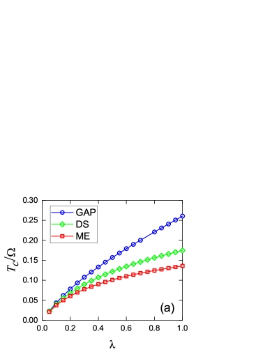
Figure 2: Numerical results of $T_{c}$. (a): using $\delta$-function of $g(\mathbf{q})$ (corresponding to $a_{0}\to 0$ limit). (b): using exponential function of $g(\mathbf{q})$. There is only a minor difference between (a) and (b). Dimensionless coupling parameter $\lambda$ is related to $g_{0}$ by the formula $g_{0}=\sqrt{\lambda}\Omega$. If $\Omega=81\mathrm{meV}$, $0.01\Omega\approx 9.5\mathrm{K}$.

Motivated by the existing experiments, the IOP-induced superconductivity has been theoretically investigated Xiang12 ; Xing14 ; Johnston-NJP2016 ; Dolgov17 ; Opp-PRB2018 by solving the ME equations of $A_{1}(\epsilon,\mathbf{p})$ and $\Delta(\epsilon,\mathbf{p})$. However, to date, there is still no consensus on the value of $T_{c}$ caused by IOPs. Different results have been obtained by different groups. The existence of controversy about $T_{c}$ is not surprising, as the kinetics and dynamics of mobile electrons in FeSe film is quite complicated. In order to acquire precise result of $T_{c}$, one needs to take into account several effects, including the potentially important contributions of vertex corrections, the multi-band electronic structure Opp-PRB2018 , the unusual screening of Coulomb interaction Millis18 , and the influence of magnetic and nematic fluctuations Yao16 . Among all of these effects, the role of vertex corrections is of special interest. Experiments Shen14 and first principles calculations Gongxg15 have confirmed that IOPs are nearly dispersionless, and the frequency $\Omega(\mathbf{q})\equiv\Omega\approx 81\mathrm{meV}$. In comparison, the Fermi energy Lee15 is roughly $E_{F}\approx 65$meV. Apparently, the Migdal theorem is no longer reliable since the ratio $\Omega/E_{F}>1$, and the impact of vertex corrections must be properly incorporated.

In this paper, we will not investigate all the effects mentioned above. Our concentration is on the influence of vertex corrections on the value of $T_{c}$. For simplicity, we consider the single band model, following Ref. Johnston-NJP2016 . It is known that the scattering due to IOPs is dominated by small-$\mathbf{q}$ forward scattering Shen14 ; Lee15 ; Johnston-NJP2016 , which is described by a coupling function $g(\mathbf{q})=g_{0}e^{-|\mathbf{q}|/q_{0}}$ where the parameter $q_{0}$ is determined by lattice constant. Similar to Ref. Johnston-NJP2016 , we consider two different forms of $g(\mathbf{q})$: $\delta$-function and exponential function. The full set of integral equations of $A_{1,2}(\epsilon,\mathbf{p})$ and $\Delta(\epsilon,\mathbf{p})$ are too complicated to solve and proper approximations are unavoidable. Since $A_{2}(\epsilon,\mathbf{p})$ can be absorbed into a redefinition of chemical potential, here we assume that $A_{2}(\epsilon,\mathbf{p})=1$. Because IOPs lead to extreme forward scattering, the initial and final states of electrons are mostly located near Fermi surface, which allows us to further set $\xi_{\mathbf{p}}=\xi_{\textbf{p}_{F}}$. As a result, the coupled equations are independent of momenta.

To separate the physical effects of the mass renormalization and the vertex corrections, we will consider three approximations: (1) the so-called GAP approximation that includes only the gap equation and ignores both mass renormalization ($A_{1}(\epsilon)=1$) and vertex corrections ($\Gamma_{t}=\sigma_{3}$); (2) the standard ME approximation that couples the equation of $A_{1}(\epsilon)$ self-consistently to that of $\Delta(\epsilon)$ but ignores all the vertex corrections ($\Gamma_{t}=\sigma_{3}$); (3) our DS equation approximation that self-consistently takes into account the mass renormalization $A_{1}(\epsilon)$ and all the vertex corrections. The corresponding equations of $A_{1}(\epsilon)$ and $\Delta(\epsilon)$ are explicitly shown in Appendix C. These equations can be numerically solved by using the iterative method, which is demonstrated in Appendix D.

The numerical results of $T_{c}$ are shown in Fig. 2. The upper, middle, and lower curves are the results obtained under GAP, DS, and ME approximations, respectively. We see that the GAP approximation overestimates $T_{c}$, whereas the ME approximation underestimates $T_{c}$. This indicates that, ignoring electron mass renormalization may improperly increase $T_{c}$ and ignoring vertex corrections may improperly reduce $T_{c}$. For very small values of $\lambda$, GAP and ME results are both good. When $\lambda$ is increasing, the deviation from DS results (middle curve) becomes progressively more dramatic. For instance, if $\lambda=0.5$, the GAP result of $T_{c}$ (denoted by $T_{c}^{\mathrm{GAP}}$) is about $32\mathrm{K}$ higher, and the ME result of $T_{c}$ (denoted by $T_{c}^{\mathrm{ME}}$) is about $20\mathrm{K}$ lower, than the DS result of $T_{c}$ (denoted by $T_{c}^{\mathrm{DS}}$). For $\lambda=1.0$, $T_{c}^{\mathrm{GAP}}-T_{c}^{\mathrm{DS}}\approx 85\mathrm{K}$ and $T_{c}^{\mathrm{DS}}-T_{c}^{\mathrm{ME}}\approx 38\mathrm{K}$. For $\lambda=2.0$ (not shown in Fig. 2), $T_{c}^{\mathrm{GAP}}-T_{c}^{\mathrm{DS}}\approx 200\mathrm{K}$ and $T_{c}^{\mathrm{DS}}-T_{c}^{\mathrm{ME}}\approx 70\mathrm{K}$. It is clear that the GAP and ME approximations are valid only in the weak-coupling regime. When $\lambda$ becomes sufficiently large, both GAP and ME approximations are quantitatively unreliable. In contrast, our DS equation approach remains well-controlled and can lead to reliable results.

The effect of Coulomb interaction is not included in the above analysis. The Coulomb interaction is usually treated by the pseudopotential method Allen ; Carbotte . After including the contribution of pseudopotential $\mu^{\ast}$, the value of $T_{c}$ would be reduced Johnston-NJP2016 by roughly $10$%-$20$%.

It is known that a nematic order, which spontaneously breaks $C_{4}$-symmetry down to $C_{2}$-symmetry, exists in bulk FeSe material Coldea17 ; Bohmer17 ; Hoffman17 . Although the physical origin of nematic order is still in fierce debate Fernandes14 , a widely accepted notion is that the nematic order is induced by electron-electron interaction, rather than lattice distortion. When monolayer FeSe is placed on SrTiO₃ substrate, nematic order is suppressed Hoffman17 , indicating that the interaction that causes nematicity should not play an important role in 1UC FeSe/SrTiO₃. But nematic fluctuation may not be negligible and could help enhance superconductivity Yao16 . Similarly, although there is no long-range magnetic order in bulk FeSe and 1UC FeSe/SrTiO₃, the spin fluctuation may mediate Cooper pairing. Recently, the cooperative effect of spin fluctuation and IOPs on superconducting $T_{c}$ in 1UC FeSe/SrTiO₃ has been studied Johnston21 using the ME formalism. It will be interesting to investigate the coupling of electrons to nematic and/or spin fluctuation by employing our DS equation approach.

The realistic electronic structure of FeSe film is more complicated than the single band model considered in our work. The multi-band effects Opp-PRB2018 ; Johnston21 cannot be ignored. The impacts of nematic and spin fluctuations also need to be examined. In this sense, our results do not provide a conclusive answer to the underlying microscopic mechanism for the remarkable $T_{c}$ enhancement. But our approach does provide a firm basis for further theoretical studies. Indeed, even if the multi-band effects and additional pairing mechanism(s) are considered, the value of $T_{c}$ cannot be determined accurately if the full EPI vertex corrections were not correctly taken into account. As shown in Fig. 2, ignoring vertex corrections leads to a considerable underestimation of $T_{c}$. Once the full vertex function is incorporated into the DS equations, one could proceed to consider the multi-band effects as well as additional pairing mechanism(s).

In the future, we will generalize our approach from the simple single-band model to more realistic multi-band models Opp-PRB2018 . The EPI vertex function may become more complex after considering the multi-band effects. The interplay of EPI and Coulomb interaction also needs to be handled more carefully. These issues will be addressed in forthcoming separate works.

VIII Summary and discussion

In summary, our DS equation approach provides a novel nonperturbative framework for the theoretical study of superconductivity induced by EPI of any strength. To testify its efficiency, it would be interesting to apply it to a number of well-defined models. As the simplest model describing EPI, Holstein model Holstein59 have been extensively investigated Scalettar89 ; Marsiglio90 ; Scalettar93 ; Johnston18 by various methods (see Ref. Johnston18 for a recent review). When EPI becomes very strong, superconductivity is not the only instability and EPI may lead to a CDW state Scalettar89 ; Marsiglio90 ; Scalettar93 ; Johnston18 . An extended version of our approach can be used to investigate the competition between superconductivity and CDW in Holstein model. The results will be presented elsewhere.

The applicability of our approach is not restricted to EPI systems. The DS equations and associated WTIs can be similarly constructed and solved if phonon is replaced by other sorts of bosons. A particularly interesting example is the U(1) gauge boson that couples strongly to gapless fermions excited around the Fermi surface of a two-dimensional strange metal Lee92 ; Nayak94 ; Polchinski94 ; Altshuler94 ; Lee09 . In this case, the vertex corrections would have more significant effects on physical quantities than EPI systems, because the function $A_{1}(\epsilon,\mathbf{p})$ exhibits singular behaviors in the ultra-low energy region. The non-Fermi liquid behavior produced by gauge interaction can be studied by solving the self-consistent integral equation of $A_{1}(\epsilon,\mathbf{p})$ and $A_{2}(\epsilon,\mathbf{p})$.

Heavy fermion system is another platform to apply our approach. The role played by phonons in heavy fermion system was studied in Ref. Jarrell10 based on a periodic Anderson model combined with Holstein model. The coherence temperature $T_{\mathrm{coh}}$ is nearly unaffected by phonons if EPI is handled within ME approximation Jarrell10 . But calculations using DFMT in concert with a continuous-time QMC impurity solver found Jarrell10 that the coupling of conduction electrons to phonons leads to a strong reduction of $T_{\mathrm{coh}}$. This indicates the complete failure of Migdal theorem in heavy fermion system, since the ratio $T_{D}/T_{\mathrm{coh}}$, $T_{D}$ being the temperature scale of Debye frequency, is no longer small. Actually, even weak EPI suffices to cause Kondo breakdown Jarrell10 . It would be of great interest to revisit this problem by using our approach and examine how these results are affected by EPI vertex corrections.

The interest of this paper is restricted to metals with a finite Fermi surface. In Dirac semimetals that exhibit zero-dimensional Fermi points, the low-energy fermionic excitations have more degrees of freedom (such as spin, sublattice, and valley). There, the vertex function should be determined by a larger number of coupled WTIs. Our approach has recently been generalized Pan20 to deal with the strong fermion-phonon interaction and long-range Coulomb interaction in Dirac semimetals.

Appendix A Functional integral rules

Our field-theoretic analysis is carried out within the framework of functional integral. To help the readers understand the analysis, in this appendix we list some basic rules of functional integration that are used in our derivation. These rules are not new and can be found in standard textbooks of quantum field theory Itzykson ; Peskin .

All the correlation functions are generated from three important quantities: the partition function $Z(\eta^{{\dagger}},\eta,J)$, the generating functional $W(\eta^{{\dagger}},\eta,J)$, and the generating functional $\Xi(\Psi,\Psi^{{\dagger}},\phi)$. They are defined as follows:

$$Z(\eta^{{\dagger}},\eta,J) = \int\mathcal{D}\phi\mathcal{D}\Psi^{{\dagger}}\mathcal{D}\Psi\exp\left(i\int\mathcal{L}(z)\right),$$ (55)

$$W(\eta^{{\dagger}},\eta,J) = -i\ln Z(\eta^{{\dagger}},\eta,J),$$ (56)

$$\Xi(\Psi,\Psi^{{\dagger}},\phi) = W(\eta^{{\dagger}},\eta,J)-\int(\eta^{{\dagger}}\Psi+\Psi^{{\dagger}}\eta+J\phi).$$

The following identities will be frequently used:

$$\frac{\delta W}{\delta J}=\langle\phi\rangle,\quad\frac{\delta W}{\delta\eta}=-\langle\Psi^{\dagger}\rangle,\quad\frac{\delta W}{\delta\eta^{\dagger}}=\langle\Psi\rangle,$$ (58)

$$\frac{\delta\Xi}{\delta\phi}=-J,\quad\frac{\delta\Xi}{\delta\Psi}=\eta^{\dagger},\quad\frac{\delta\Xi}{\delta\Psi^{\dagger}}=-\eta.$$ (59)

$W(\eta^{{\dagger}},\eta,J)$ generates all the connected Green’s functions and $\Xi(\Psi,\Psi^{{\dagger}},\phi)$ generates all the irreducible proper vertices of electron-phonon coupling. For instance, the full electron propagator $G(z-z^{\prime})$ and full phonon propagator $F(z-z^{\prime})$ are given by

$$G(z-z^{\prime}) \equiv -i\langle\Psi(z)\Psi^{\dagger}(z^{\prime})\rangle=\frac{\delta^{2}W}{\delta\eta^{\dagger}(z)\delta\eta(z^{\prime})},$$ (60)

$$F(z-z^{\prime}) \equiv -i\langle\phi(z)\phi^{\dagger}(z^{\prime})\rangle=-\frac{\delta^{2}W}{\delta J(z)\delta J(z^{\prime})}.$$ (61)

With the help of Eqs. (58-59), the above two expressions are calculated by the following steps:

$$\frac{\delta^{2}W}{\delta\eta^{\dagger}(z)\delta\eta(z^{\prime})} = -\frac{\delta\Psi^{\dagger}(z^{\prime})}{\delta\eta^{\dagger}(z)}=-\left(\frac{\delta\eta^{\dagger}(z)}{\delta\Psi^{\dagger}(z^{\prime})}\right)^{-1}$$ (62)

$$= -\left(\frac{\delta^{2}\Xi}{\delta\Psi^{{\dagger}}(z^{\prime})\delta\Psi(z)}\right)^{-1},$$

$$\frac{\delta^{2}W}{\delta J(z)\delta J(z^{\prime})} = \frac{\delta\phi(z^{\prime})}{\delta J(z)}=\left(\frac{\delta J(z)}{\delta\phi(z^{\prime})}\right)^{-1}$$ (63)

$$= -\left(\frac{\delta^{2}\Xi}{\delta\phi(z^{\prime})\delta\phi(z)}\right)^{-1}.$$

Here it is important to emphasize that $\frac{\delta^{2}W}{\delta\eta^{{\dagger}}\delta\eta}$ and $\frac{\delta^{2}W}{\delta J\delta J}$ only involve connected Feynman diagrams for the electron and phonon propagators. To understand this, we take the phonon field $\phi$ as an example, and perform functional derivatives as follows:

$$\frac{\delta^{2}W}{\delta J\delta J} = -i\frac{\delta}{\delta J}\left(\frac{1}{Z}\int\mathcal{D}\phi\mathcal{D}\Psi\mathcal{D}\Psi^{\dagger}i\phi\exp\{i\mathcal{L}\}\right)$$ (64)

$$= i\frac{\int\mathcal{D}\phi\mathcal{D}\Psi\mathcal{D}\Psi^{\dagger}\phi\phi\exp\{i\mathcal{L}\}}{Z}$$

$$-i\left(\frac{\int\mathcal{D}\phi\mathcal{D}\Psi\mathcal{D}\Psi^{\dagger}\phi\exp\{i\mathcal{L}\}}{Z}\right)^{2}.$$

In the last line, the first term contains all the connected and disconnected diagrams, whereas the second term contains all the disconnected diagrams. Hence, the phonon propagator $F=-\frac{\delta^{2}W}{\delta J\delta J}$ contains only connected diagrams. The same is true for the electron propagator, namely $G=\frac{\delta^{2}W}{\delta\eta^{{\dagger}}\delta\eta}$ contains only connected diagrams.

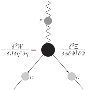
Figure 3: Diagrammatic illustration of the relation given by Eq. (4). Dropping three external legs of $3$-point correlation function $\langle\phi\Psi\Psi^{\dagger}\rangle$ yields the EPI vertex function $\Gamma_{\mathrm{v}}$.

The correlation function $\langle\phi\Psi\Psi^{\dagger}\rangle$ is expressed as follows

$$\langle\phi\Psi\Psi^{\dagger}\rangle\equiv\frac{\delta^{3}W}{\delta J\delta\eta^{\dagger}\delta\eta}=-FG\frac{\delta^{3}\Xi}{\delta\phi\delta\Psi^{\dagger}\delta\Psi}G,$$ (65)

where we have defined a truncated (external legs being removed) EPI vertex function $\Gamma_{\mathrm{v}}$, i.e.,

$$\Gamma_{\mathrm{v}}(z_{1},z_{2},z_{3})\equiv\frac{\delta^{3}\Xi}{\delta\phi(z_{1})\delta\Psi^{\dagger}(z_{2})\delta\Psi(z_{3})}.$$ (66)

These two equations are schematically illustrated by Fig. (3). Analogous to the electron and phonon propagators, here the vertex function $\Gamma_{\mathrm{v}}$ receives contributions solely from connected diagrams. It is straightforward to define and analyze four-point and higher-point correlation functions by means of similar operations. However, for our purposes it suffices to consider two- and three-point correlation functions. For a more comprehensive illustration of functional integral techniques, we would refer readers to the textbook of Itzykson and Zuber Itzykson .

Appendix B Dyson-Schwinger equations of fermion and boson propagators

In this appendix, we derive the formal DS integral equations of the full fermion propagator $G(p)$ and the full phonon propagator $F(q)$ by using the rules of functional integral presented in Appendix A.

First derive the DS equation of electron propagator. The derivation is based on an apparent fact that the partition function is invariant under an arbitrary infinitesimal variation of spinor field $\Psi^{{\dagger}}$, that is

$$\int\mathcal{D}\phi\mathcal{D}\Psi^{{\dagger}}\mathcal{D}\Psi\frac{\delta}{i\delta\Psi^{\dagger}}\exp\{iS\}=0.$$

It is easy to get

$$\langle(i\sigma_{0}\partial_{t}-\sigma_{3}\xi_{\partial_{\mathbf{z}}})\Psi(z)-g\phi(z)\sigma_{3}\Psi(z)+\eta(z)\rangle=0.$$ (67)

Using the relations given by Eq. (58), we re-write the above equation as

$$-\eta(z)=(i\sigma_{0}\partial_{t}-\sigma_{3}\xi_{\partial_{\mathbf{z}}})\frac{\delta W}{\delta\eta^{\dagger}(z)}+ig\sigma_{3}\frac{\delta^{2}W}{\delta J(z)\delta\eta^{\dagger}(z)}-g\frac{\delta W}{\delta J(z)}\sigma_{3}\frac{\delta W}{\delta\eta^{\dagger}(z)}.$$ (68)

The last term of r.h.s. vanishes upon removing sources and can be directly omitted. Operating functional derivative of both sides with respect to $\eta(z_{2})$ yields

$$\delta(z-z_{2})\sigma_{0} = (i\sigma_{0}\partial_{t}-\sigma_{3}\xi_{\partial_{\mathbf{z}}})\frac{\delta^{2}W}{\delta\eta^{\dagger}(z)\delta\eta(z_{2})}+ig\sigma_{3}\frac{\delta^{3}W}{\delta J(z)\delta\eta^{\dagger}(z)\delta\eta(z_{2})}$$

$$= (i\sigma_{0}\partial_{t}-\sigma_{3}\xi_{\partial_{\mathbf{z}}})G(z-z_{2})-ig\int dz_{1}^{\prime}dz_{2}^{\prime}\sigma_{3}F(z-z_{1}^{\prime})G(z-z^{\prime})\frac{\delta^{3}\Xi}{\delta\phi(z_{1}^{\prime})\delta\Psi^{\dagger}(z^{\prime})\delta\Psi(z_{2}^{\prime})}G(z_{2}^{\prime}-z_{2}).$$

This expression can be re-written as

$$G^{-1}(z-z_{3}) = (i\sigma_{0}\partial_{t}-\sigma_{3}\xi_{\partial_{\mathbf{z}}})\delta(z-z_{3})-ig\int dz_{1}^{\prime}dz^{\prime}\sigma_{3}F(z-z_{1}^{\prime})G(z-z^{\prime})\frac{\delta^{3}\Xi}{\delta\phi(z_{1}^{\prime})\delta\Psi^{\dagger}(z^{\prime})\delta\Psi(z_{3})}.$$ (69)

Making use of the definition

$$\Gamma_{\mathrm{v}}(z_{1}^{\prime},z^{\prime},z_{3})\equiv\frac{\delta^{3}\Xi}{\delta\phi(z_{1}^{\prime})\delta\Psi^{\dagger}(z^{\prime})\delta\Psi(z_{3})}$$ (70)

and performing Fourier transformation to Eq. (69), we ultimately obtain the following DS equation for fermion propagator $G(p)$:

$$G^{-1}(p)=G_{0}^{-1}(p)-ig\int dq\sigma_{3}G(p+q)F(q)\Gamma_{\mathrm{v}}(q,p).$$ (71)

The Fourier transformation of $\Gamma_{\mathrm{v}}(z_{1}^{\prime},z^{\prime},z_{3})$ is

$$\Gamma_{\mathrm{v}}(q,p)=\int dz_{1}^{\prime}dz^{\prime}e^{ip(z_{1}^{\prime}-z_{3})}e^{-i(p+q)(z_{1}^{\prime}-z^{\prime})}\Gamma_{\mathrm{v}}(z_{1}^{\prime},z^{\prime},z_{3}).$$

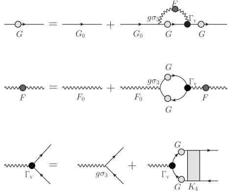
Figure 4: An intuitive diagrammatic illustration of the coupled DS equations of $G(p)$, $F(q)$, and $\Gamma_{\mathrm{v}}(q,p)$. The complicated relation of these three functions can be readily seen. The connection between $K_{4}(p,p^{\prime},q)$ and higher-point correlation functions are not shown.

The DS integral equation of $F(q)$ is derived based on the fact that the partition function is invariant under an arbitrary infinitesimal variation of phonon field $\phi$, i.e.,

$$\int\mathcal{D}\phi\mathcal{D}\Psi^{{\dagger}}\mathcal{D}\Psi\frac{\delta}{i\delta\phi}\exp\{iS\}=0.$$

Then one finds that

$$\langle\mathbb{D}_{z}\phi(z)-g\Psi^{\dagger}(z)\sigma_{3}\Psi(z)+J(z)\rangle=0.$$ (72)

Again, we use the relations of Eq. (58) to obtain

$$-J(z) = \mathbb{D}_{z}\langle\phi(z)\rangle+ig\mathrm{Tr}\left[\sigma_{3}\frac{\delta^{2}W}{\delta\eta^{\dagger}(z)\delta\eta(z)}\right]$$ (73)

$$-g\mathrm{Tr}\left[\sigma_{3}\frac{\delta W}{\delta\eta^{\dagger}(z)}\frac{\delta W}{\delta\eta(z)}\right].$$

Here a trace operator is introduced to operate on the components of Nambu spinors. The last term of r.h.s. vanishes upon removing external sources and can be directly omitted. This expression can be re-written, using rules of functional integral, as

$$\frac{\delta\Xi}{\delta\phi(z)}=\mathbb{D}_{z}\langle\phi(z)\rangle-ig\mathrm{Tr}\left[\sigma_{3}\left(\frac{\delta^{2}\Xi}{\delta\Psi^{{\dagger}}(z)\delta\Psi(z)}\right)^{-1}\right].$$

Performing functional derivative of both sides of this equation with respect to the field $\phi(z^{\prime})$ gives rise to

$$\frac{\delta^{2}\Xi}{\delta\phi(z)\delta\phi(z^{\prime})}=\mathbb{D}_{z}\delta(z-z^{\prime})+ig\int dz_{1}dz_{2}\mathrm{Tr}\left[\sigma_{3}\left(\frac{\delta^{2}\Xi}{\delta\Psi^{{\dagger}}(z_{1})\delta\Psi(z)}\right)^{-1}\left(\frac{\delta^{3}\Xi}{\delta\phi(z^{\prime})\delta\Psi^{{\dagger}}(z_{1})\delta\Psi(z_{2})}\right)\left(\frac{\delta^{2}\Xi}{\delta\Psi^{{\dagger}}(z)\delta\Psi(z_{2})}\right)^{-1}\right].$$

Making use of the identities given by Eqs. (60-63), we obtain

$$F^{-1}(z-z^{\prime})=\mathbb{D}_{z}\delta(z-z^{\prime})+ig\int dz_{1}dz_{2}\mathrm{Tr}\left[\sigma_{3}G(z-z_{1})\Gamma(z^{\prime},z_{1},z_{2})G(z_{2}-z)\right],$$ (74)

which, after carrying our Fourier transformation according to Eq. (B), becomes

$$F^{-1}(q)=F_{0}^{-1}(q)+ig\int_{p}\mathrm{Tr}\left[\sigma_{3}G(p+q)\Gamma_{\mathrm{v}}(q,p)G(p)\right].$$

(75)

This is the DS equation of the full boson propagator.

The DS equations of the EPI vertex function $\Gamma_{\mathrm{v}}(q,p)$ can be derived by performing a series of analogous calculations Itzykson . The derivation is quite lengthy and the details will not be explicitly presented here. For a more understandable diagrammatic illustration of the coupled DS equations of $G(p)$, $F(q)$, and $\Gamma_{\mathrm{v}}(q,p)$, please see Fig. 4. The DS equation of $\Gamma_{\mathrm{v}}(q,p)$ can be formally written as

$$\Gamma_{\mathrm{v}}(q,p) = g\sigma_{3}-\int_{p^{\prime}}G(p^{\prime}+q)\Gamma_{\mathrm{v}}(q,p^{\prime})G(p^{\prime})K_{4}(p,p^{\prime},q).$$

Here, the function $K_{4}(p,p^{\prime},q)$ is defined via the $4$-point correlation function $\langle\phi\phi^{{\dagger}}\Psi\Psi^{{\dagger}}\rangle$ as follows:

$$FFK_{4}GG=\langle\phi\phi^{{\dagger}}\Psi\Psi^{{\dagger}}\rangle.$$

One could verify that, the function $K_{4}(p,p^{\prime},q)$ satisfies its own DS integral equation, which in turn is related to other higher-point correlation functions. In fact, there exists an infinite number of DS equations that connect every $n$-point correlation function to a $(n+1)$-point correlation function for all positive integers $n>1$. All of these DS equations are self-consistently coupled. Therefore, the full set of DS equations are not closed and cannot be tackled. For this reason, although the full set of DS equations are exact and, in principle, contain all the interaction-induced effects, they are rarely used in the realistic studies on strongly correlated electron systems. Fortunately, we have shown in the main paper that the DS equation of electron propagator $G(p)$ is indeed self-closed if several symmetry-induced exact identities are properly taken into account. The full boson propagator $F(q)$ and the vertex function $\Gamma_{\mathrm{v}}(q,p)$ can be obtained from the numerical solutions of $G(p)$.

Appendix C Gap equations in small-$\mathbf{q}$ dominated EPI systems

In 1UC FeSe/SrTiO₃, electrons in FeSe film couple to IOPs. Different from ordinary (acoustic) phonons, IOPs are nearly dispersionless. The dispersion $\Omega_{\mathbf{q}}$ can thus be taken as a constant. This type of EPI is sharply peaked at $\mathbf{q}=0$ Shen14 ; Lee15 ; Johnston-NJP2016 ; Dolgov17 ; Opp-PRB2018 . We will make use of this unique feature to simplify the vertex function $\Gamma_{t}(q,p)$, which then reduces the time required to complete the numerical computation. Moreover, if one is mainly interested in the determination of $T_{c}$, it is reasonable to linearize the DS equations, i.e., taking the $\Delta\to 0$ limit, near $T_{c}$.

As discussed in Sec. VII, here we will consider three different approximations, namely GAP, ME, and DS approximations, of the coupled integral functions of $A_{1}(\epsilon)$ and $\Delta(\epsilon)$. To compare to results reported in Ref. Johnston-NJP2016 , we also consider two different forms of coupling function $g(\mathbf{q})$: an idealized $\delta$-function and a more realistic exponential function. We adopt Matsubara formalism to describe finite-temperature correlation functions. The electron frequency is $\epsilon_{n}=(2n+1)\pi T$ and the phonon frequency is $\omega_{m}=2m\pi T$, where $n$ and $m$ are integers.

C.1 $\delta$-function

In the case of $\delta$-function, the coupling function has the simple form $g(\mathbf{q})=g_{0}\delta(\mathbf{q})$. Under GAP approximation, we take $A_{1}=1$. Then there is only the equation of pairing function:

$$\Delta(\epsilon_{n})=\lambda\Omega^{2}T\sum_{m}\frac{2\Omega}{\Omega^{2}+\omega_{m}^{2}}\frac{\Delta(\epsilon_{n}+\omega_{m})}{(\epsilon_{n}+\omega_{m})^{2}+\Delta^{2}(\epsilon_{n}+\omega_{m})}.$$

(77)

The dimensionless coupling constant $\lambda$ is related to EPI coupling constant $g_{0}$ by $g_{0}=\sqrt{\lambda}\Omega$. This approximation ignores the mass renormalization and supposes that EPI leads only to Cooper pairing. The gap equation given by Eq. (77) is similar, but not identical to, the standard BCS gap equation. This equation has previously been analyzed by Rademaker et al. Johnston-NJP2016 , who made a comparison between the solution of Eq. (77) to that of the standard BCS gap equation and shown that extreme forward scattering leads to a remarkable enhancement of $T_{c}$.

Certainly, it is inappropriate to neglect the contributions of $A_{1}$. If both $A_{1}$ and $\Delta$ are considered, we would obtain the following two coupled ME equations:

$$\Delta(\epsilon_{n}) = \lambda\Omega^{2}T\sum_{m}\frac{2\Omega}{\Omega^{2}+\omega_{m}^{2}}\frac{\Delta(\epsilon_{n}+\omega_{m})}{A_{1}^{2}(\epsilon_{n}+\omega_{m})(\epsilon_{n}+\omega_{m})^{2}+\Delta^{2}(\epsilon_{n}+\omega_{m})},$$ (78)

$$A_{1}(\epsilon_{n}) = 1+\frac{1}{\epsilon_{n}}\lambda\Omega^{2}T\sum_{m}\frac{2\Omega}{\Omega^{2}+\omega_{m}^{2}}\frac{\epsilon_{n}+\omega_{m}}{A_{1}^{2}(\epsilon_{n}+\omega_{m})(\epsilon_{n}+\omega_{m})^{2}+\Delta^{2}(\epsilon_{n}+\omega_{m})}.$$ (79)

Including the full vertex corrections, described by $\Gamma_{t}$, to the above ME equations leads to the following two DS equations

$$\Delta(\epsilon_{n}) = \lambda\Omega^{2}T\sum_{m}\frac{2\Omega}{\Omega^{2}+\omega_{m}^{2}}\frac{\Delta(\epsilon_{n}+\omega_{m})}{A_{1}^{2}(\epsilon_{n}+\omega_{m})(\epsilon_{n}+\omega_{m})^{2}+\Delta^{2}(\epsilon_{n}+\omega_{m})}\frac{A_{1}(\epsilon_{n}+\omega_{m})(\epsilon_{n}+\omega_{m})-A_{1}(\epsilon_{n})\epsilon_{n}}{\omega_{m}},$$ (80)

$$A_{1}(\epsilon_{n}) = 1+\frac{1}{\epsilon_{n}}\lambda\Omega^{2}T\sum_{m}\frac{2\Omega}{\Omega^{2}+\omega_{m}^{2}}\frac{A_{1}(\epsilon_{n}+\omega_{m})(\epsilon_{n}+\omega_{m})}{A_{1}^{2}(\epsilon_{n}+\omega_{m})(\epsilon_{n}+\omega_{m})^{2}+\Delta^{2}(\epsilon_{n}+\omega_{m})}\frac{A_{1}(\epsilon_{n}+\omega_{m})(\epsilon_{n}+\omega_{m})-A_{1}(\epsilon_{n})\epsilon_{n}}{\omega_{m}}.$$

C.2 Exponential function

We then consider the more realistic exponential function of coupling parameter $g(\mathbf{q})=\sqrt{\lambda}\Omega e^{-\mathbf{q}/q_{0}}$. It is necessary to introduce an UV cutoff $\Lambda$, which then can be used to define a dimensionless parameter $r=q_{0}/\Lambda$. Under the GAP approximation, the pure gap equation is given by

$$\Delta(\epsilon_{n}) = \left(\frac{2}{r}\right)^{2}\lambda\Omega^{2}T\sum_{m}\int_{0}^{1}dxx\exp\left(-\frac{2x}{r}\right)\frac{2\Omega}{\Omega^{2}+\omega_{m}^{2}}$$ (82)

$$\times\frac{\Delta(\epsilon_{n}+\omega_{m})}{\sqrt{(\epsilon_{n}+\omega_{m})^{2}+\Delta^{2}(\epsilon_{n}+\omega_{m})}\sqrt{(\epsilon_{n}+\omega_{m})^{2}+\Delta^{2}(\epsilon_{n}+\omega_{m})+\zeta x^{2}}}.$$

The coupled ME equations of $\Delta(\epsilon_{n})$ and $A_{1}(\epsilon_{n})$ are

$$\Delta(\epsilon_{n}) = \left(\frac{2}{r}\right)^{2}\lambda\Omega^{2}T\sum_{m}\int_{0}^{1}dxx\exp\left(-\frac{2x}{r}\right)\frac{2\Omega}{\Omega^{2}+\omega_{m}^{2}}$$ (83)

$$\times\frac{\Delta(\epsilon_{n}+\omega_{m})}{\sqrt{A_{1}^{2}(\epsilon_{n}+\omega_{m})(\epsilon_{n}+\omega_{m})^{2}+\Delta^{2}(\epsilon_{n}+\omega_{m})}\sqrt{A_{1}^{2}(\epsilon_{n}+\omega_{m})(\epsilon_{n}+\omega_{m})^{2}+\Delta^{2}(\epsilon_{n}+\omega_{m})+\zeta x^{2}}},$$

$$A_{1}(\epsilon_{n}) = 1+\frac{1}{\epsilon_{n}}\left(\frac{2}{r}\right)^{2}\lambda\Omega^{2}T\sum_{m}\int_{0}^{1}dxx\exp\left(-\frac{2x}{r}\right)\frac{2\Omega}{\Omega^{2}+\omega_{m}^{2}}$$ (84)

$$\times\frac{A_{1}(\epsilon_{n}+\omega_{m})(\epsilon_{n}+\omega_{m})}{\sqrt{A_{1}^{2}(\epsilon_{n}+\omega_{m})(\epsilon_{n}+\omega_{m})^{2}+\Delta^{2}(\epsilon_{n}+\omega_{m})}\sqrt{A_{1}^{2}(\epsilon_{n}+\omega_{m})(\epsilon_{n}+\omega_{m})^{2}+\Delta^{2}(\epsilon_{n}+\omega_{m})+\zeta x^{2}}}.$$

After including vertex corrections, the coupled DS equations are of the form

$$\Delta(\epsilon_{n}) = \left(\frac{2}{r}\right)^{2}\lambda\Omega^{2}T\sum_{m}\int_{0}^{1}dxx\exp\left(-\frac{2x}{r}\right)\frac{2\Omega}{\Omega^{2}+\omega_{m}^{2}}$$ (85)

$$\times\frac{\Delta(\epsilon_{n}+\omega_{m})}{\sqrt{A_{1}^{2}(\epsilon_{n}+\omega_{m})(\epsilon_{n}+\omega_{m})^{2}+\Delta^{2}(\epsilon_{n}+\omega_{m})}\sqrt{A_{1}^{2}(\epsilon_{n}+\omega_{m})(\epsilon_{n}+\omega_{m})^{2}+\Delta^{2}(\epsilon_{n}+\omega_{m})+\zeta x^{2}}}$$

$$\times\frac{A_{1}(\epsilon_{n}+\omega_{m})(\epsilon_{n}+\omega_{m})-A_{1}(\epsilon_{n})\epsilon_{n}}{\omega_{m}},$$

$$A_{1}(\epsilon_{n}) = 1+\frac{1}{\epsilon_{n}}\left(\frac{2}{r}\right)^{2}\lambda\Omega^{2}T\sum_{m}\int_{0}^{1}dxx\exp\left(-\frac{2x}{r}\right)\frac{2\Omega}{\Omega^{2}+\omega_{m}^{2}}$$ (86)

$$\times\frac{A_{1}(\epsilon_{n}+\omega_{m})(\epsilon_{n}+\omega_{m})}{\sqrt{A_{1}^{2}(\epsilon_{n}+\omega_{m})(\epsilon_{n}+\omega_{m})^{2}+\Delta^{2}(\epsilon_{n}+\omega_{m})}\sqrt{A_{1}^{2}(\epsilon_{n}+\omega_{m})(\epsilon_{n}+\omega_{m})^{2}+\Delta^{2}(\epsilon_{n}+\omega_{m})+\zeta x^{2}}}$$

$$\times\frac{A_{1}(\epsilon_{n}+\omega_{m})(\epsilon_{n}+\omega_{m})-A_{1}(\epsilon_{n})\epsilon_{n}}{\omega_{m}}.$$

Appendix D Numerical method

The self-consistent integral function(s) can be solved numerically by using the iterative method. Let us take Eqs. (85-86) as an example to illustrate how the iterative method works. In the first step, one assumes some initial values of $A_{1}$ and $\Delta$. In the second step, substitute these initial values into Eqs. (85-86) to obtain a set of new values of $A_{1}$ and $\Delta$, which are more or less different from the initial values. In the third step, substitute the new values again into Eqs. (85-86) to obtain another set of new values of $A_{1}$ and $\Delta$. Repeat this manipulation many times until the input and output of $A_{1}$ and $\Delta$ no longer change. Such stable values of $A_{1}$ and $\Delta$ are precisely the solutions that we need.

The two equations contain a summation over $\omega_{m}$ for all possible values of $m$. In practice, it is not possible, nor necessary, to sum to infinity. On generic physical grounds we know that $A_{1}$ and $\Delta$ are positive even functions of frequency. Smaller frequency gives rise to larger $A_{1}$ and $\Delta$. When electron frequency is much larger than phonon frequency $\Omega$, the contributions are negligible. We choose a large number $N=400$ and define $\epsilon_{n}$ as follows

$$\epsilon_{n}=\pm(2n-1)\pi T,\quad n=1,2,...,N.$$ (87)

Introduce $\omega_{m}^{\prime}$ and define it as $\omega^{\prime}_{m}=\epsilon_{n}+\omega_{m}$. Thus $\omega^{\prime}_{m}$ is restricted to the same region as $\epsilon_{n}$, namely

$$\omega^{\prime}_{m}=\pm(2m-1)\pi T, m=1,2,...,N.$$ (88)

Then Eqs. (C9-C10) can be expressed as

$$\Delta(\epsilon_{n}) = \left(\frac{2}{r}\right)^{2}\lambda\Omega^{2}T\sum_{m=1}^{N}\int_{0}^{1}dxx\exp\left(-\frac{2x}{r}\right)\frac{2\Omega}{\Omega^{2}+(\omega^{\prime}_{m}-\epsilon_{n})^{2}}$$ (89)

$$\times\frac{\Delta(\omega^{\prime}_{m})}{\sqrt{A_{1}^{2}(\omega^{\prime}_{m}){\omega^{\prime}_{m}}^{2}+\Delta^{2}(\omega^{\prime}_{m})}\sqrt{A_{1}^{2}(\omega^{\prime}_{m}){\omega^{\prime}_{m}}^{2}+\Delta^{2}(\omega^{\prime}_{m})+\zeta x^{2}}}\frac{A_{1}(\omega^{\prime}_{m})\omega^{\prime}_{m}-A_{1}(\epsilon_{n})\epsilon_{n}}{\omega^{\prime}_{m}-\epsilon_{n}},$$

$$A_{1}(\epsilon_{n}) = 1+\frac{1}{\epsilon_{n}}\left(\frac{2}{r}\right)^{2}\lambda\Omega^{2}T\sum_{m=1}^{N}\int_{0}^{1}dxx\exp\left(-\frac{2x}{r}\right)\frac{2\Omega}{\Omega^{2}+(\omega^{\prime}_{m}-\epsilon_{n})^{2}}$$ (90)

$$\times\frac{A_{1}(\omega^{\prime}_{m})\omega^{\prime}_{m}}{\sqrt{A_{1}^{2}(\omega^{\prime}_{m}){\omega^{\prime}_{m}}^{2}+\Delta^{2}(\omega^{\prime}_{m})}\sqrt{A_{1}^{2}(\omega^{\prime}_{m}){\omega^{\prime}_{m}}^{2}+\Delta^{2}(\omega^{\prime}_{m})+\zeta x^{2}}}\frac{A_{1}(\omega^{\prime}_{m})\omega^{\prime}_{m}-A_{1}(\epsilon_{n})\epsilon_{n}}{\omega^{\prime}_{m}-\epsilon_{n}}.$$

Now choose two initial values for unknown functions $A_{1}$ and $\Delta$: $A_{1}=1$ and $\Delta=10^{-3}$. The Gaussian quadrature is used to integrate over variable $x$. After $i$ times of iteration, we would obtain $A_{1,i}$ and $\Delta_{i}$, which are then substituted into the above two equations to obtain $A_{1,i+1}$ and $\Delta_{i+1}$. Repeat such calculations until the difference between $i$-results and $(i+1)$-results vanishes. $A_{1,i+1}$ and $\Delta_{i+1}$ are related to $A_{1,i}$ and $\Delta_{i}$ via the following equations:

$$\Delta_{i+1}(n) = \left(\frac{2}{r}\right)^{2}\lambda\Omega^{2}T\sum_{m=1}^{N}\int_{0}^{1}dxx\exp\left(-\frac{2x}{r}\right)\frac{2\Omega}{\Omega^{2}+4\pi^{2}T^{2}(m-n)^{2}}$$ (91)

$$\times\frac{\Delta_{i}(m)}{\sqrt{A_{1,i}^{2}(m)(2m-1)^{2}\pi^{2}T^{2}+\Delta_{i}^{2}(m)}\sqrt{A_{1,i}^{2}(m)(2m-1)^{2}\pi^{2}T^{2}+\Delta_{i}^{2}(m)+\zeta x^{2}}}$$

$$\times\frac{A_{1,i}(m)(2m-1)-A_{1,i}(n)(2n-1)}{2(m-n)}$$

$$+\left(\frac{2}{r}\right)^{2}\lambda\Omega^{2}T\sum_{m=1}^{N}\int_{0}^{1}dxx\exp\left(-\frac{2x}{r}\right)\frac{2\Omega}{\Omega^{2}+4\pi^{2}T^{2}(m+n)^{2}}$$

$$\times\frac{\Delta_{i}(m)}{\sqrt{A_{1,i}^{2}(m)(2m-1)^{2}\pi^{2}T^{2}+\Delta_{i}^{2}(m)}\sqrt{A_{1,i}^{2}(m)(2m-1)^{2}\pi^{2}T^{2}+\Delta_{i}^{2}(m)+\zeta x^{2}}}$$

$$\times\frac{A_{1,i}(m)(2m-1)+A_{1,i}(n)(2n-1)}{2(m+n)},$$

$$A_{1,i+1}(n) = 1+\frac{1}{(2n-1)}\left(\frac{2}{r}\right)^{2}\lambda\Omega^{2}T\sum_{m=1}^{N}\int_{0}^{1}dxx\exp\left(-\frac{2x}{r}\right)\frac{2\Omega}{\Omega^{2}+4\pi^{2}T^{2}(m-n)^{2}}$$ (92)

$$\times\frac{A_{1,i}(m)(2m-1)}{\sqrt{A_{1,i}^{2}(m)(2m-1)^{2}\pi^{2}T^{2}+\Delta_{i}^{2}(m)}\sqrt{A_{1,i}^{2}(m)(2m-1)^{2}\pi^{2}T^{2}+\Delta_{i}^{2}(m)+\zeta x^{2}}}$$

$$\times\frac{A_{1,i}(m)(2m-1)-A_{1,i}(n)(2n-1)}{2(m-n)}$$

$$-\frac{1}{(2n-1)}\left(\frac{2}{r}\right)^{2}\lambda\Omega^{2}T\sum_{m=1}^{N}\int_{0}^{1}dxx\exp\left(-\frac{2x}{r}\right)\frac{2\Omega}{\Omega^{2}+4\pi^{2}T^{2}(m+n)^{2}}$$

$$\times\frac{A_{1,i}(m)(2m-1)}{\sqrt{A_{1,i}^{2}(m)(2m-1)^{2}\pi^{2}T^{2}+\Delta_{i}^{2}(m)}\sqrt{A_{1,i}^{2}(m)(2m-1)^{2}\pi^{2}T^{2}+\Delta_{i}^{2}(m)+\zeta x^{2}}}$$

$$\times\frac{A_{1,i}(m)(2m-1)+A_{1,i}(n)(2n-1)}{2(m+n)}.$$

The error factors created after $i$ times of iteration are

$$\mathrm{EPS}_{a}(i)=\frac{1}{N}\sum_{n=1}^{N}\frac{|A_{1,i}(n)-A_{1,i-1}(n)|}{|A_{1,i}(n)|+|A_{1,i-1}(n)|},\quad\mathrm{EPS}_{b}(i)=\frac{1}{N}\sum_{n=1}^{N}\frac{|\Delta_{i}(n)-\Delta_{i-1}(n)|}{|\Delta_{i}(n)|+|\Delta_{i-1}(n)|}.$$ (93)

For given values of $\lambda$ and $T$, both $\mathrm{EPS}_{a}(i)$ and $\mathrm{EPS}_{b}(i)$ decrease gradually with increasing $i$, provided that $\Delta$ has nontrivial solutions. When $\mathrm{EPS}_{a}(i)$ and $\mathrm{EPS}_{b}(i)$ become sufficiently small, the iteration can be terminated and the finial results of $A_{1}$ and $\Delta$ are obtained. In realistic calculations, we take $\mathrm{EPS}_{a}<10^{-6}$ and $\mathrm{EPS}_{b}<10^{-6}$ as the criterion for achieving convergence. If $\Delta$ does not have a nontrivial solution, $\mathrm{EPS}_{a}$ still becomes gradually small, but $\mathrm{EPS}_{b}$ does not tend to decrease with growing $i$. Actually, $\Delta_{i}(n)$ would rapidly go to zero as $i$ grows. Once $\Delta_{i}(n)$, which takes a finite initial value, becomes sufficiently small, we would take $\Delta(n)=0$ directly and terminate the iterating process. In practice, the iteration procedure can be terminated if $\frac{1}{N}\sum_{n=1}^{N}\Delta_{i}(n)<10^{-9}$.

References

• (1) J. R. Schrieffer, Theory of Superconductivity (CRC Press, 2018).
• (2) A. A. Abrikosov, L. P. Gor’kov, and I. Y. Dzyaloshinskii, Quantum Field Theoretical Methods in Statistical Physics (Pergamon Press, 1965).
• (3) D. J. Scalapino, The electron-phonon interaction and strong-coupling superconductivity, in Superconductivity, edited by R. D. Parks (Marcel Dekker, New York, 1969).
• (4) A. Migdal, Interaction between electrons and lattice vibrations in a normal metal, Sov. Phys. JETP 7, 996 (1958).
• (5) G. M. Eliashberg, Interactions between electrons and lattice vibrations in a superconductor, Sov. Phys. JETP 11, 696 (1960).
• (6) P. B. Allen and B. MitroviΔ‡, Theory of Superconducting Tc, Solid State Physics, Vol.37 (Academic Press, 1982).
• (7) J. P. Carbotte, Properties of boson-exchange superconductors, Rev. Mod. Phys. 62, 1027 (1990).
• (8) F. Marsiglio, Eliashberg theory: A short review, Ann. Phys. 417, 168102 (2020).
• (9) Q.-Y. Wang, Z. Li, W.-H. Zhang, Z.-C. Zhang, J.-S. Zhang, W. Li, H. Ding, Y.-B. Ou, P. Deng, K. Chang, J. Wen, C.-L. Song, K. He, J.-F. Jia, S.-H. Ji, Y.-Y. Wang, L.-L. Wang, X. Chen, X.-C. Ma, and Q.-K. Xue, Interface-induced high-temperature superconductivity in single unit-cell FeSe films on SrTiO3, Chin. Phys. Lett. 29, 037402 (2012).
• (10) J. J. Lee, F. T. Schmitt, R. G. Moore, S. Johnston, Y.-T. Cui, W. Li, M. Yi, Z. K. Liu, M. Hashimoto, Y. Zhang, D. H. Lu, T. P. Devereaux, D.-H. Lee, and Z.-X. Shen, Interfacial mode coupling as the origin of the enhancement of $T_{c}$ in FeSe films on SrTiO3, Nature (London), 515, 245 (2014).
• (11) D.-H. Lee, What makes the $T_{c}$ of FeSe/SrTiO3 so high? Chinese Phys. 24, 117405 (2015).
• (12) L. P. Gor’kov, Peculiarities of superconductivity in the single-layer FeSe/SrTiO3 interface, Phys. Rev. B 93, 060507(R) (2016).
• (13) L. Rademaker et al., Enhanced superconductivity due to forward scattering in FeSe thin films on SrTiO3 substrates, New J. Phys. 18, 022001 (2016).
• (14) I. Martin, MoirΓ© superconductivity, Ann. Phys. 417, 168118 (2020).
• (15) S. Engelsberg and J. R. Schrieffer, Coupled Electron-Phonon System, Phys. Rev. 131, 993 (1963).
• (16) A. S. Alexandrov, Breakdown of the Migdal-Eliashberg theory in the strong-coupling adiabatic regime, Europhys. Lett. 56, 92 (2001).
• (17) I. Esterlis, B. Nosarzewski, E. W. Huang, B. Moritz, T. P. Devereaux, D. J. Scalapino, and S. A. Kivelson, Breakdown of the Migdal-Eliashberg theory: A determinant quantum Monte Carlo study, Phys. Rev. B 97, 140501(R) (2018).
• (18) J. F. Schooley, W. R. Hosler, and M. L. Cohen, Superconductivity in semiconducting SrTiO3, Phys. Rev. Lett. 12, 474 (1964).
• (19) M. N. Gastiasoro, A. V. Chubukov, and R. M. Fernandes, Phonon-mediated superconductivity in low carrier-density systems, Phys. Rev. B 99, 094524 (2019).
• (20) Y. Cao, V. Fatemi, S. Fang, K. Watanabe, T. Taniguchi, E. Kaxiras and P. Jarillo-Herrero, Unconventional superconductivity in magic-angle graphene superlattices, Nature 556, 43 (2018).
• (21) O. Gunnarsson, Superconductivity in fullerides, Rev. Mod. Phys. 69, 575 (1997).
• (22) E. Cappelluti, C. Grimaldi, L. Pietronero, S. StrΓ€ssler, and G.A. Ummarino, Superconductivity of Rb3C60: breakdown of the Migdal-Eliashberg theory, Eur. Phys. J. B 21, 383 (2001).
• (23) T. Cuk, D. H. Lu, X. J. Zhou, Z.-X. Shen, T. P. Devereaux, and N. Nagaosa, A review of electron-phonon coupling seen in the high-Tc superconductors by angle-resolved photoemission studies (ARPES), phys. stat. sol. (b) 242, 11 (2005).
• (24) Y. Nambu, Quasi-particles and gauge invariance in the theory of superconductivity, Phys. Rev. 117, 648 (1960).
• (25) C. Itzykson and J.-B. Zuber, Quantum Field Theory (McGraw-Hill, New York, 1980).
• (26) Y. Takahashi, in Quantum Field Theory, edited by F. Mancini, (Elsevier Science Publisher, 1986).
• (27) K.-I. Kondo, Transverse Ward-Takahashi identity, anomaly, and Schwinger-Dyson equation, Int. J. Mod. Phys. A, 12, 5651 (1997).
• (28) H. He, F. C. Khanna, and Y. Takahashi, Transverse Ward-Takahashi identity for the fermion-boson vertex in gauge theories, Phys. Lett. B 480, 222 (2000).
• (29) P. A. M. Dirac, Discussion of the infinite distribution of electrons in the theory of the positron, Proc. Camb. Phil. Soc. 30, 150 (1934).
• (30) R. Peierls, The vacuum in Dirac’s theory of the positive electron, Proc. Roy. Soc. Series A 146, 420 (1934).
• (31) R. Serber, A note on positron theory and proper energies, Phys. Rev. 49, 545 (1936).
• (32) J. Schwinger, On gauge invariance and vacuum polarization, Phys. Rev. 82, 664 (1951).
• (33) R. Jackiw and K. Johnson, Anomalies of the axial-vector current, Phys. Rev. 182, 1459 (1969).
• (34) C. G. Callan, S. Coleman, and R. Jackiw, A new improved energy-momentum tensor, Ann. Phys. 59, 42 (1970).
• (35) W. A. Bardeen, Anonmalous Ward identities in spinor field theories, Phys. Rev. 184, 1848 (1969).
• (36) M. E. Peskin and D. V. Schroeder, An Introduction to Quantum Field Theory (CRC Press, 2019).
• (37) J. Novotny and M. Schnabl, Point-splitting regularization of composite operators and anomalies, Fortschr. Phys. 48, 253 (2000).
• (38) P. W. Anderson, Plasmons, gauge invariance, and mass, Phys. Rev. 130, 439 (1963).
• (39) P. W. Higgs, Broken symmetries and the masses of gauge bosons, Phys. Rev. Lett. 13, 508 (1964).
• (40) F. F. Assaad and H. G. Evertz, World-line and determinantal quantum Monte Carlo methods for spins, phonons and electrons, Lect. Notes Phys. 739, 277 (2008).
• (41) A. Georges, G. Kotliar, W. Krauth, and M. J. Rozenberg, Dynamical mean-field theory of strongly correlated fermion systems and the limit of infinite dimensions, Rev. Mod. Phys. 68, 13 (1996).
• (42) F.-C. Hsu, J.-Y. Luo, K.-W. Yeh, T.-K. Chen, T.-W. Huang, P. M. Wu, Y.-C. Lee, Y.-L. Huang, Y.-Y. Chu, D.-C. Yan, and M.-K. Wu, From the cover: Superconductivity in the PbO-type structure FeSe, Proc. Natl. Acad. Sci. USA 105, 14262 (2008).
• (43) S. N. Rebec, T. Jia, C. Zhang, M. Hashimoto, D.-H. Lu, R. G. Moore, and Z.-X. Shen, Coexistence of replica bands and superconductivity in FeSe monolayer films, Phys. Rev. Lett. 118, 067002 (2017).
• (44) Y.-Y. Xiang, F. Wang, D. Wang, Q.-H. Wang, and D.-H. Lee, High-temperature superconductivity at the FeSe/SrTiO3 interface, Phys. Rev. B 86, 134508 (2012).
• (45) B. Li, Z. W. Xing, G. Q. Huang, and D. Y. Xing, Electron-phonon coupling enhanced by the FeSe/SrTiO3 interface, J. Appl. Phys. 115, 193907 (2014).
• (46) M. L. KuliΔ‡ and O. V. Dolgov, The electron-phonon interaction with forward scattering peak is dominant in high $T_{c}$ superconductors of FeSe films on SrTiO3 (TiO2), New J. Phys. 19, 013020 (2017).
• (47) A. Aperis and P. M. Oppeneer, Multiband full-bandwidth anisotropic Eliashberg theory of interfacial electron-phonon coupling and high-$T_{c}$ superconductivity in FeSe/SrTiO3, Phys. Rev. B 97, 060501(R) (2018).
• (48) Y. Zhou and A. J. Millis, Dipolar phonons and electronic screening in monolayer FeSe on SrTiO3, Phys. Rev. B 96, 054516 (2017).
• (49) Z.-X. Li, F. Wang, D.-H. Lee, and H. Yao, What makes the $T_{c}$ of monolayer FeSe on SrTiO3 so high: a sign-problem-free quantum Monte Carlo study, Sci. Bull. 61, 925 (2016).
• (50) Y. Xie, H.-Y. Cao, Y. Zhou, S. Chen, H. Xiang, and X.-G. Gong, Oxygen vacancy induced flat phonon mode at FeSe/SrTiO3 interface, Sci. Rep. 5, 10011 (2015).
• (51) A. Coldea and M. D. Watson, The Key Ingredients of the Electronic Structure of FeSe, Ann. Rev. Condens. Matter Phys. 9, 125 (2018).
• (52) A. E. BΓΆhmer and A. Kreisel, Nematicity, magnetism and superconductivity in FeSe, J. Phys. Condens. Matter 30, 023001 (2017).
• (53) D. Huang and J. E. Hoffman, Monolayer FeSe on SrTiO3, Annu. Rev. Condens. Matter Phys. 8, 311 (2017).
• (54) R. M. Fernandes, A. V. Chubukov, and J. Schmalian, What Drives Nematic Order in Iron-Based Superconductors?, Nat. Phys. 10, 97 (2014).
• (55) L. Rademaker, G. Alvarez-Suchini, K. Nakatsukasa, Y. Wang, S. Johnston, Enhanced superconductivity in FeSe/SrTiO3 from the combination of forward scattering phonons and spin fluctuations, arXiv:2101.08307.
• (56) T. Holstein, Studies of polaron motion: Part I. The molecular-crystal model, Ann. Phys. 8, 325 (1959).
• (57) P. Niyaz, J. E. Gubernatis, R. T. Scalettar, and C. Y. Fong, Charge-density-wave-gap formation in the two-dimensional Holstein model at half-filling, Phys. Rev. B 48, 16011 (1993).
• (58) R. T. Scalettar, N. E. Bickers, and D. J. Scalapino, Competition of pairing and Peierls-charge-density-wave correlations in a two-dimensional electron-phonon model, Phys. Rev. B 40, 197 (1989).
• (59) F. Marsiglio, Pairing and charge-density-wave correlations in the Holstein model at half-filling, Phys. Rev. B 42, 2416 (1990).
• (60) P. M. Dee, K. Nakatsukasa, Y. Wang, and S. Johnston, Temperature-filling phase diagram of the two-dimensional Holstein model in the thermodynamic limit by self-consistent Migdal approximation, Phys. Rev. B 99, 024514 (2018).
• (61) P. A. Lee and N. Nagaosa, Gauge theory of the normal state of high-$T_{c}$ superconductors, Phys. Rev. B 46, 5621 (1992).
• (62) C. Nayak and F Wilczek, Non-Fermi liquid fixed point in $2+1$ dimensions, Nucl. Phys. B 417, 359 (1994).
• (63) J. Polchinski, Low-energy dynamics of the spinon-gauge system, Nucl. Phys. B 422, 617 (1994).
• (64) B. L. Altshuler, L. B. Ioffe, and A. J. Millis, Low-energy properties of fermions with singular interactions, Phys. Rev. B 50, 14048 (1994).
• (65) S.-S. Lee, Low-energy effective theory of Fermi surface coupled with U(1) gauge field in $2+1$ dimensions, Phys. Rev. B 80, 165102 (2009).
• (66) M. Raczkowski, P. Zhang, F. F. Assaad, T. Pruschke, and M. Jarrell, Phonons and the coherence scale of models of heavy fermions, Phys. Rev. B 81, 054444 (2010).
• (67) X.-Y. Pan, Z.-K. Yang, X. Li, and G.-Z. Liu, Nonperturbative Dyson-Schwinger equation approach to strongly interacting Dirac fermion systems, arXiv:2003.10371.