Preserving privacy enables “co-existence equilibrium” of competitive diffusion in social networks

Abstract

With the advent of social media, different companies often promote competing products simultaneously for word-of-mouth diffusion and adoption by users in social networks. For such scenarios of competitive diffusion, prior studies show that the weaker product will soon become extinct (i.e., “winner takes all”). It is intriguing to observe that in practice, however, competing products, such as iPhone and Android phone, often co-exist in the market. This discrepancy may result from many factors such as the phenomenon that a user in the real world may not spread its use of a product due to dissatisfaction of the product or privacy protection. In this paper, we incorporate users’ privacy for spreading behavior into competitive diffusion of two products and develop a problem formulation for privacy-aware competitive diffusion. Then we prove that privacy-preserving mechanisms can enable a “co-existence equilibrium” (i.e., two competing products co-exist in the equilibrium) in competitive diffusion over social networks. In addition to the rigorous analysis, we also demonstrate our results with experiments over real network topologies.

I Introduction

The advent of social media has generated tremendous interest in ways that companies use social networks to maximize product adoption by consumers [1, 2, 3]. One particular method of product promotion is viral marketing via word-of-mouth effects [4]. In word-of-mouth marketing applications, given users’ limited attention span [5], different companies often promote competing products simultaneously in a social network using diffusion; i.e., there is a process of competitive diffusion on the social network [6]. For example, Apple may try to promote its new iPhone, while Samsung tries to advertise its new Galaxy phone.

Recently, it has garnered much interest to study how competing products spread in a social network [7, 1, 8, 9, 10, 3]. In the diffusion of a pair of competing products, one significant result by Prakash et al. [8] shows that “winner takes all”, or, more accurately, the weaker product will soon become extinct. A similar result is also given by Wei et al. [3]. The studies [8, 3] provide an insightful understanding of how competing products propagate among users via social networks. It is intriguing to observe that in practice, however, competing products often co-exist in the market. For example, iPhone and Android phones both have a large number of users. Figure 1, generated from Google Trends, shows the time evolution of worldwide search-interests in iPhone and Android over the past 5 years. It is clear from the plot that interests in iPhone and Android co-exist in the market. We remark that this co-existence is the result of many real-world factors (e.g., companies can advertise the products directly to customers), so its analysis can be complex. Yet, the purpose of this example is to simply provide an intuitive understanding for the co-existence of competing products in the real world.

Figure 1: Global search-interests in iPhone and Android over the past 5 years, generated from Google Trends${}^{\text{\ref{footnote-google}}}$. Numbers represent search interest relative to the highest point on the chart. A value of 100 is the peak popularity for the term. A value of 50 means that the term is half as popular.

The “winner-takes-all” result by [8, 3] assumes that each user after adopting a product will positively spread the product to her social friends. In contrast, competing products co-exist in the real world, and one may attribute this co-existence to the fact that a consumer using a product currently may be dissatisfied with the product and thus be unwilling to spread the product to her friends. In fact, the user may even spread negative belief about the product that she is using [11]. Further, this can be understood from a privacy perspective: a user may hesitate to disclose her product adoption due to privacy concerns so she may choose to not spread her product or even choose to spread the competing product with some probability. We now provide a simple example for illustration. Consider a couple’s use of smart phones. The wife holds an iPhone, while the husband uses an Android phone. The husband feels disappointed about his Android phone, and is told by the wife that she is happy with her iPhone. Hence, even when the husband still carries his Android phone for some time and is not an iPhone user himself, he may recommend iPhone to his colleagues at work given the good experience of his wife. We can understand the husband’s behavior from a privacy viewpoint: the husband would like to hide his use of an Android phone and thus recommend iPhone instead of Android to his colleagues.

Our model, building on the notion of privacy, is broad enough to represent the fact that a user may not spread her product adoption (even when the underlying reason is not because of privacy concern, but due to frustration of her product). Furthermore, users today are indeed concerned about privacy, especially for social networking where massive amounts of personal data are generated and prone to adversarial attacks [8, 12].

Motivated to formally show that competing products can co-exist in the network, we consider the problem of privacy-aware competitive diffusion, where two products compete for adoption by users located in a social network. Individual users are privacy-aware in the sense that an individual using a product may pretend adopting another product and spread the latter product to her social friends.

Our contributions can be summarized as follows:

• We formulate a problem called privacy-aware competitive diffusion, where products compete for adoption by privacy-aware users in a social network.

• We show that incorporating privacy into competitive diffusion can enable the co-existence of competing products (specifically, the probability of any user adopting any product is non-zero in the equilibrium), while it is known that traditional (privacy-oblivious) competitive diffusion exhibits the “winner-takes-all” phenomenon.

To provide more formal understanding, we present model details and main results below.

Models for privacy-aware competitive diffusion. We consider the diffusion model of $\textrm{Susceptible-}\textrm{Infected}_{1}\textrm{-Infected}_{2}\textrm{-Susceptible}$ (i.e., $S{I_{1}}{I_{2}}S$), which extends the widely studied “flu-like” Susceptible-Infected-Susceptible (i.e., $SIS$) model from one product to the case of two competing products, so that each user in a social network can be in one of the following three states: Susceptible (healthy), $I_{1}$ (using product 1), or $I_{2}$ (using product 2). Let $\sigma_{1}$ (resp., $\sigma_{2}$) denote the spreading strength (i.e., the infection rate divided by the healing rate) of product 1 (resp., product 2); more details can be found in Section III-A on Page III-A later. A user’s private data indicates which product she is using. To protect user’s privacy, we consider:

• for $j\in\{1,2\}$, each user adopting product $j$ spreads product $1$ to its friends with probability $r_{j1}$, spreads product $2$ to its friends with probability $r_{j2}$, and does not spread any product with probability $1-r_{j1}-r_{j2}$;

• each user not yet adopting any product does not advocate any product.

The above model is in the same spirit as the randomized response technique [13] that was introduced to protect users’ privacy during survey interviews. We represent the privacy parameters by a matrix $\begin{bmatrix}r_{11}&r_{12}&1-r_{11}-r_{12}\\ r_{21}&r_{22}&1-r_{21}-r_{22}\end{bmatrix}$, and refer to this matrix as the privacy scheme. Note that we always require each $r_{\bullet\bullet}$ in the matrix to be strictly positive, whereas $1-r_{j1}-r_{j2}$ can take $0$ or be greater than $0$. Formally, we always enforce

$$\begin{Bmatrix}0<r_{11}<1,~{}~{}&~{}~{}0<r_{12}<1,\\ 0<r_{21}<1,~{}~{}&~{}~{}0<r_{22}<1,\\ r_{11}+r_{12}\leq 1,~{}~{}&~{}~{}r_{21}+r_{22}\leq 1.\end{Bmatrix}$$ (1)

A privacy scheme $\begin{bmatrix}r_{11}&r_{12}&1-r_{11}-r_{12}\\ r_{21}&r_{22}&1-r_{21}-r_{22}\end{bmatrix}$ is perfect if $r_{11}=r_{21}$ and $r_{12}=r_{22}$ (i.e., the first row and the second row of the matrix are exactly the same). The intuition is that a user’s private state, corresponding to adopting which product, is completely hidden from her spreading behavior. In a perfect privacy scheme, we write the same-valued $r_{11}$ and $r_{21}$ as $\gamma_{1}$, and write the same-valued $r_{12}$ and $r_{22}$ as $\gamma_{2}$ so that the privacy scheme becomes $\begin{bmatrix}\gamma_{1}&\gamma_{2}&1-\gamma_{1}-\gamma_{2}\\ \gamma_{1}&\gamma_{2}&1-\gamma_{1}-\gamma_{2}\end{bmatrix}$ and the condition (1) becomes

$$\begin{Bmatrix}0<\gamma_{1}<1,~{}~{}~{}~{}~{}~{}~{}0<\gamma_{2}<1,~{}~{}~{}~{}~{}~{}~{}\gamma_{1}+\gamma_{2}\leq 1.\end{Bmatrix}.$$ (2)

We always enforce (2) for a perfect privacy scheme.

Main results. We summarize the main results as ① and ② below, and provide more details later. We emphasize that all results are for undirected social networks and the $S{I_{1}}{I_{2}}S$ model described above. The conclusions can be different for other models.

• For a connected social network with an arbitrary topology, there exist perfect privacy schemes $\begin{bmatrix}\gamma_{1}~{}&\gamma_{2}~{}&1-\gamma_{1}-\gamma_{2}\\ \gamma_{1}~{}&\gamma_{2}~{}&1-\gamma_{1}-\gamma_{2}\end{bmatrix}$ satisfying (2) to enable a co-existence equilibrium of two competing products.

• For a social network with a complete graph topology, there exist general privacy schemes $\begin{bmatrix}r_{11}&r_{12}&1-r_{11}-r_{12}\\ r_{21}&r_{22}&1-r_{21}-r_{22}\end{bmatrix}$ satisfying (1) to enable a co-existence equilibrium of two competing products.

Comparing ① and ② above, we see that ① considers a more general network topology while requiring a more restrictive privacy scheme, whereas ② considers a more general privacy scheme at the sacrifice of a more restrictive network topology. Below we explain ① and ②, respectively.

Further remarks on Result ①. We can formally state the above result ① as follows. For a connected social network with an arbitrary topology, let $\lambda$ be the largest eigenvalue of the adjacency matrix. Then ① means that under a privacy scheme $\begin{bmatrix}\gamma_{1}&\gamma_{2}&1-\gamma_{1}-\gamma_{2}\\ \gamma_{1}&\gamma_{2}&1-\gamma_{1}-\gamma_{2}\end{bmatrix}$ satisfying (2), if

$$\sigma_{1}\gamma_{1}+\sigma_{2}\gamma_{2}>1/\lambda,$$ (3)

the system will reach a stable equilibrium where both products co-exist. More specifically, in this equilibrium, the probability of any user adopting any product is positive. In contrast, if the sign “$>$” in the condition (3) is replaced by “$<$”, the system will reach a stable equilibrium where both products die out.

Further remarks on Result ②. We now explain the above result ②. Result ② applies to general privacy schemes and hence overcomes the limitation of ① which requires privacy schemes to be perfect. However, Result ② is only for complete graph topologies, while ① addresses arbitrary topologies. Formally, we have the following for result ②: for a social network of $n$ nodes with a complete graph topology, under a privacy scheme $\begin{bmatrix}r_{11}&r_{12}&1-r_{11}-r_{12}\\ r_{21}&r_{22}&1-r_{21}-r_{22}\end{bmatrix}$, if

$$\frac{1}{2}\left[\begin{array}[]{l}\sigma_{1}r_{11}+\sigma_{2}r_{22}\\[2.0pt] +\sqrt{(\sigma_{1}r_{11}-\sigma_{2}r_{22})^{2}+4\sigma_{1}\sigma_{2}r_{12}r_{21}}\end{array}\right]>\frac{1}{n-1},$$ (6)

then the system will reach a stable co-existence equilibrium; if the sign “$>$” in the condition (6) is replaced by “$<$”, the system will reach a stable equilibrium where both products die out. Compared with $1/\lambda$ on the right hand side of (3), the right hand side of (6) is $\frac{1}{n-1}$ since the largest eigenvalue of the adjacency matrix for a complete graph of $n$ nodes is $n-1$, as explained in Footnote 5 later on Page 5.

Note that the above results all involve the largest eigenvalue of the adjacency matrix of the underlying social network. This comes from the eigenvalue-based approach of analyzing stable equilibria of dynamical systems discussed below.

Technical approach. We use the standard approach of analyzing stable equilibria of dynamical systems [14] (Nevertheless, the analysis is still challenging as discussed in the next paragraph). With $\boldsymbol{x}$ denoting the state vector which contains the probability of each user adopting each product, we have a dynamical system comprising differential equations in the form of $\overset{\boldsymbol{{.}}}{\boldsymbol{x}}=G(\boldsymbol{x},\boldsymbol{\alpha})$, where $\overset{\boldsymbol{{.}}}{\boldsymbol{x}}$ is the derivative of $\boldsymbol{x}$ (with respect to the time $t$), and $\boldsymbol{\alpha}$ is the parameter vector. Then the equilibria are defined to have a zero derivative and thus are obtained by solving $G(\boldsymbol{x},\boldsymbol{\alpha})=\boldsymbol{0}$. Afterwards, an equilibrium $\boldsymbol{x}_{*}$ is stable if each eigenvalue of the Jacobian matrix at $\boldsymbol{x}_{*}$ has a strictly negative real part, where the Jacobian matrix is an $m\times m$ matrix with the element in the $i$th row and $j$th column being $\frac{\partial\overset{\boldsymbol{{.}}}{{x_{i}}}}{\partial x_{j}}$, if the state vector $\boldsymbol{x}$ has $m$ dimensions: $x_{1},x_{2},\ldots,x_{m}$ (i.e., $\boldsymbol{x}=[x_{1},x_{2},\ldots,x_{m}]$). Finally, if the goal is to show that the system will reach a stable equilibrium where both products co-exist, we prove that there is only one stable equilibrium and this equilibrium gives a state vector whose elements are all strictly positive. If the goal is to show that the system will reach a stable equilibrium where both products die out, we prove that there is only one stable equilibrium and this equilibrium gives a state vector whose elements are all zero.

Challenge. Although the above approach is standard, the analysis is nontrivial. One main difficulty lies in analyzing the Jacobian matrix and its eigenvalues to show the stability of an equilibrium. In our privacy-aware competitive diffusion problem, the Jacobian matrix has many non-zero elements, making it difficult to evaluate its eigenvalues. In our setting with arbitrary network topologies, dealing with the $2n\times 2n$ Jacobian matrix further complicates the analysis. In prior privacy-oblivious competitive diffusion studies, the Jacobian matrix has many zero elements and is much easier to tackle.

The rest of the paper is organized as follows. Section II surveys related work. Then we present the system model in Section III, and the main results in Section IV. Afterwards, we provide in Section V experiments to confirm the analytical results. In Sections VI, we discuss the proof ideas for establishing the main results. We conclude the paper in Section VII. Many technical details are given in the appendices.

II Related Work

Single-meme diffusion. Numerous studies have addressed single-meme diffusion, where the notion of meme is a generic term for the information propagating on the network. For the diffusion model of “flu-like” Susceptible-Infected-Susceptible (i.e., $SIS$), Wang et al. [15] presented an approximate analysis and showed that the epidemic threshold in a network equals the reciprocal of the largest eigenvalue of the network’s adjacency matrix. This result was formally proved by Van Mieghem et al. [16]. Van Mieghem [17] further derived the expression for the steady-state fraction of infected nodes. We refer interested readers to a survey [18] for more related work on single-meme diffusion.

Competitive diffusion. Prakash et al. [8] studied the $\textrm{Susceptible-}\textrm{Infected}_{1}\textrm{-Infected}_{2}\textrm{-Susceptible}$ (i.e., $S{I_{1}}{I_{2}}S$) diffusion problem for a pair of competing products and show that “winner takes all” (more accurately, the weaker product will soon become extinct). Wei et al. [3] observed an analogous result in the setting where two products propagate on two different networks defined on the same set of users. Fazeli et al. [1] considered two companies competing to maximize the consumption of their products by users which decide consumption based on best response dynamics. The goal of [1] was to investigate whether a firm with a limited budget should spend on the quality of the product or on initial seeding in the network. Bimpikis et al. [7] also considered firms’ optimal strategies under competitive diffusion and investigated their connections with the underlying social network structure. Alon [19] used a game to model the competition between many products (i.e., possibly more than two) for diffusion on a social network, and obtained the relation between the existence of pure Nash equilibria and the diameter of the network. Beutel et al. [20] modified the $S{I_{1}}{I_{2}}S$ model to allow a user to be in both $I_{1}$ and $I_{2}$ states (note that we use the standard $S{I_{1}}{I_{2}}S$ model where a user can be in only one state), and showed that competing products can co-exist in the equilibrium. However, this nice work [20] had the following limitations: 1) its theoretical result was only for a complete graph (i.e., a full clique) although their experiments consider more general topologies; and 2) [20] lacked a proof to show that the equilibrium is stable (proving the stability of an equilibrium is often much more challenging than finding an equilibrium [8]). Compared with our work, all the above reference [8, 3, 1, 7, 19] did not take users’ privacy into consideration.

Few recent studies on privacy-aware diffusion. So far, there has been only few work [21, 22, 23] recently on privacy-aware diffusion. Giakkoupis et al. [21] presented a distributed algorithm for privacy-aware information diffusion in social networks, where each user’s privacy means her opinion on the information and is modeled by how likely she forwards the information (the information itself is not perturbed). If the user favors the information, she forwards the information with higher probability compared with the case where she dislikes the information. Giakkoupis et al. [21] showed that the information spreads to a constant fraction of the network if it appeals to a constant fraction of users, and dies out if few users likes it. Harrane et al. [22] recently used privacy-aware diffusion to solve distributed inference problems, where privacy means that each user’s measurement is perturbed before being propagated to its neighbors. Zhu et al. [23] considered private link exchange over social networks, where a user’s private information is her friend list and she obfuscates the list before sending it to her neighbors to preserve privacy. Different from our work here, these recent studies [21, 22, 23] did not consider competition between different information in diffusion and their privacy signals were different from our privacy signal that captures which product the user adopts.

Notably, Krishnamurthy and Wills [24] reported a longitudinal study of diffusion of users’ private data. Avgerou and Stamatiou [25] developed a game theory framework to show that social networks help spread privacy consciousness to large populations. Akcora et al. [26] proposed a measure to quantify the risk of disclosing private information in social networks. Heatherly et al. [12] investigated how to utilize released social networking data to infer undisclosed private information about users. Baden et al. [27] presented an online social network called Persona where users’ privacy can be protected via cryptographic techniques.

III System Model

In what follows, we present the system model in detail. In Section III-A, we review traditional competitive diffusion, where user privacy is not considered. In Section III-B, we incorporate user privacy into competitive diffusion to introduce the novel problem of privacy-aware competitive diffusion. Since one may tempt to convert privacy-aware competitive diffusion into traditional (privacy-oblivious) competitive diffusion, we will elaborate on why this approach does not work at the end of this section.

III-A Traditional (Privacy-Oblivious) Competitive Diffusion

We review traditional competitive diffusion that does not take into consideration of user privacy. In particular, we look at the scenario where two competing products spread on a social network according to the following diffusion model. The diffusion model $S{I_{1}}{I_{2}}S$ extends the widely studied “flu-like” $SIS$ model from one product to the case of two products. Each user in the network can be in one of the following three states: Susceptible (healthy), $I_{1}$ (adopting product 1), or $I_{2}$ (adopting product 2).

We now describe several parameters of the $S{I_{1}}{I_{2}}S$ model. For convenience, we still use the words “infection” and “healing” as in the case of disease diffusion, although the diffused information is product adoption.

Infection rates: $\beta_{1}$ and $\beta_{2}$. A healthy user gets infected by her infected neighbors, and the infection rate of product 1 (resp., product 2) is denoted by $\beta_{1}$ (resp., $\beta_{2}$). Specifically, an infected user transmits her adoption of product 1 (resp., product 2) to each of its neighbors independently at rate $\beta_{1}$ (resp., $\beta_{2}$). In other words, the time taken for each infected user to spread product 1 (resp., product 2) to a neighbor is exponentially distributed with parameter $\beta_{1}$ (resp., $\beta_{2}$).

Healing rates: $\delta_{1}$ and $\delta_{2}$. If a user is in state $I_{1}$ (resp., $I_{2}$), she recovers on her own with rate $\delta_{1}$ (resp., $\delta_{2}$). In other words, the time taken for a user infected by product 1 (resp., product 2) to heal is exponentially distributed with parameter $\delta_{1}$ (resp., $\delta_{2}$). After a user is healed, it can get infected by product 1 or product 2 again.

Note that the infection rates $\beta_{1}$ and $\beta_{2}$, and the healing rates $\delta_{1}$ and $\delta_{2}$ are common across all users in the network; i.e., all rates are homogeneous with respect to users. This is an assumption widely made in many diffusion studies [8, 3, 1, 7, 20] to have tractable analyses. Removing this assumption to consider the heterogeneity of the infection and healing rates across users will be an interesting direction, yet the analysis may become intractable.

Dividing the infection rate by the healing rate, we obtain the spreading strengths of products 1 and 2 given by $\sigma_{1}\stackrel{{\scriptstyle\text{def}}}{{=}}\frac{\beta_{1}}{\delta_{1}}$ and $\sigma_{2}\stackrel{{\scriptstyle\text{def}}}{{=}}\frac{\beta_{2}}{\delta_{2}}$, respectively. In the network, each product competes with the other product for healthy victims. We also assume full mutual immunity: a user can not be infected by two products at the same time.

III-B Privacy-Aware Competitive Diffusion

We now present our model for privacy-aware competitive diffusion. Two products compete for adoption by users in a connected social network. A user’s private data indicates which product she is using. Users are privacy-aware in the sense that an user using a product may pretend adopting another product and spread the latter product to her social friends. We thus incorporate privacy into the above $S{I_{1}}{I_{2}}S$ diffusion problem as follows.

The technique here to preserve users’ privacy is conceptually similar to the randomized response technique [13], introduced first for survey interviews. For each user adopting product $1$ (i.e., in state $I_{1}$), her action has the following three possibilities: (i) she spreads product $1$ to her neighbors with probability $r_{11}$; (ii) she pretends that she is using product $2$ and diffuses product $2$ to her neighbors with probability $r_{12}$; (iii) she does not spread any product with probability $1-r_{11}-r_{12}$. Similarly, for a user adopting product $2$ (i.e., in state $I_{2}$), her action has the following three possibilities: (i) she spreads product $2$ to her neighbors with probability $r_{22}$; (ii) she pretends that she is using product $1$ and disseminates product $1$ to her neighbors with probability $r_{21}$; (iii) she does not spread any product with probability $1-r_{21}-r_{22}$. Finally, for a user that has not yet adopted any product, she does not advocate any product.

We represent the privacy parameters by a matrix $\begin{bmatrix}r_{11}&r_{12}&1-r_{11}-r_{12}\\ r_{21}&r_{22}&1-r_{21}-r_{22}\end{bmatrix}$, and refer to this matrix as the privacy scheme. When $r_{11}=1$, $r_{12}=0$, $r_{21}=0$, and $r_{22}=1$, the problem reduces to the traditional (i.e., privacy-oblivious) competitive diffusion problem $S{I_{1}}{I_{2}}S$ studied by Prakash et al. [8]. In the rest of paper, we focus on privacy-aware competitive diffusion and thus assume that $r_{11}$, $r_{12}$, $r_{21}$, and $r_{22}$ are strictly positive. More formally, we always enforce the condition (1) given on Page 1; i.e., $r_{11},r_{12},r_{21},r_{22}\in(0,1)$ and $r_{11}+r_{12}\leq 1$, $r_{21}+r_{22}\leq 1$.

In the literature, a widely accepted privacy definition is the renowned notion of differential privacy [28, 29, 30, 31]. Specifically, $\epsilon$-differential privacy for a mechanism that provides a randomized answer for a query on a database means that if a single record changes in the database, then the probability that the same answer is given differs by at most a multiplicative factor of $e^{\epsilon}$ (smaller $\epsilon$ means better privacy). In our privacy-aware competitive diffusion problem, each user’s private signal is her state (which is one of the three states: ${I_{1}}$, ${I_{2}}$, and $S$) and the randomized output is the state that corresponds to the product that she advocates. More relevant to our setting is the local model of differential privacy [32, 33], where each individual maintains its own data (a database of size 1) and answers only the question about the data in a differentially private manner.

Built on the above, the privacy-preserving mechanism $\begin{bmatrix}r_{11}&r_{12}&1-r_{11}-r_{12}\\ r_{21}&r_{22}&1-r_{21}-r_{22}\end{bmatrix}$ in competitive diffusion achieves $\epsilon$-(local) differential privacy for $\epsilon$ given by

$$\epsilon:=\ln\max\left\{\begin{array}[]{l}{\frac{r_{11}}{r_{21}},~{}\frac{r_{21}}{r_{11}},~{}\frac{r_{12}}{r_{22}},~{}\frac{r_{22}}{r_{12}}},\\[6.0pt] {\frac{1-r_{11}-r_{12}}{1-r_{21}-r_{22}},~{}\frac{1-r_{21}-r_{22}}{1-r_{11}-r_{12}}}\end{array}\right\}.$$ (9)

If $r_{11}=r_{21}$ and $r_{12}=r_{22}$, then $\epsilon=0$; i.e., the scheme has perfect privacy if the first row and the second row of the privacy matrix are the same. In such case, user’s spreading behavior is independent of her private state.

Problem Statement. We now state the research problem of privacy-aware competitive diffusion. Given a connected social network and the diffusion parameters (the infection rate $\beta_{1}$ and the healing rate $\delta_{1}$ for product 1, and the infection rate $\beta_{2}$ and the healing rate $\delta_{2}$ for product 2), our goal is to find a privacy scheme $\begin{bmatrix}r_{11}&r_{12}&1-r_{11}-r_{12}\\ r_{21}&r_{22}&1-r_{21}-r_{22}\end{bmatrix}$ such that competing products co-exist in the stable equilibrium.

Answer. Our answer to the above problem is different for different network topologies. Specifically, for a connected social network with an arbitrary topology, we consider perfect privacy schemes $\begin{bmatrix}\gamma_{1}&\gamma_{2}&1-\gamma_{1}-\gamma_{2}\\ \gamma_{1}&\gamma_{2}&1-\gamma_{1}-\gamma_{2}\end{bmatrix}$; for a social network with a complete graph topology, we consider general privacy schemes $\begin{bmatrix}r_{11}&r_{12}&1-r_{11}-r_{12}\\ r_{21}&r_{22}&1-r_{21}-r_{22}\end{bmatrix}$.

Privacy-aware competitive diffusion cannot be converted into traditional (privacy-oblivious) competitive diffusion. One may tempt to convert privacy-aware competitive diffusion into traditional (privacy-oblivious) competitive diffusion. For example, one may consider a privacy-oblivious diffusion problem $S{I_{1}}{I_{2}}S$, where product 1 has an infection rate of $\beta_{1}r_{11}+\beta_{2}r_{21}$ and a healing rate of $\delta_{1}$, and product 2 has an infection rate of $\beta_{1}r_{12}+\beta_{2}r_{22}$ and a healing rate of $\delta_{2}$, and treat this problem as an equivalent of our privacy-aware diffusion problem $S{I_{1}}{I_{2}}S$. This approach does not work as explained below. In the privacy-oblivious diffusion problem, if at some point a product dies out, then the product becomes extinct forever and cannot be reborn again. However, in our privacy-aware diffusion problem, even if at some point an product is wiped out, the product may revive again, because some users adopting the other product may pretend using this product and spread this product to its neighbors, which can resurrect the product.

IV Main Results

We present the main results in this section. We present conditions for a stable co-existence equilibrium in Section IV-A, and conditions for no stable co-existence equilibrium in Section IV-B. The notion of a stable co-existence equilibrium means that competing products co-exist in a equilibrium which is also stable (i.e., attracting), and the co-existence is in the strong sense: the probability of any user adopting any product is positive (i.e., greater than $0$) in the stable equilibrium.

IV-A Conditions for a Stable Co-Existence Equilibrium

To have a stable co-existence equilibrium, we discuss in Theorem 1 privacy schemes on a connected social network with an arbitrary topology, and present in Theorem 2 general privacy schemes on a social network with a complete graph topology.

Theorem 1 (Perfect Privacy Schemes on Arbitrary Network Topologies).

Consider a connected social network with an arbitrary topology, with $\lambda$ denoting the largest eigenvalue of the adjacency matrix. For the privacy-aware $SI_{1}I_{2}S$ problem with a perfect privacy scheme $\begin{bmatrix}\gamma_{1}&\gamma_{2}&1-\gamma_{1}-\gamma_{2}\\ \gamma_{1}&\gamma_{2}&1-\gamma_{1}-\gamma_{2}\end{bmatrix}$ satisfying $\gamma_{1},\gamma_{2}\in(0,1)$ and $\gamma_{1}+\gamma_{2}\leq 1$, if

$$\sigma_{1}\gamma_{1}+\sigma_{2}\gamma_{2}>1/\lambda,$$ (10)

then the system will reach a stable co-existence equilibrium.

Remark 1.

In Remark 5 of Theorem 3 later, we will show that if the sign “$>$” in the condition (10) is replaced by “$<$”, the system will reach a stable equilibrium where both products die out.

We explain the basic ideas and the corresponding challenges to establish Theorem 1 in Section VI-B on Page VI-B. The proof details are given in Appendix B-B on Page B-B.

Theorem 2 (General Privacy Schemes on Complete Network Topologies).

Consider a social network of $n$ nodes with a complete graph topology. For the privacy-aware $SI_{1}I_{2}S$ problem with a general privacy scheme $\begin{bmatrix}r_{11}&r_{12}&1-r_{11}-r_{12}\\ r_{21}&r_{22}&1-r_{21}-r_{22}\end{bmatrix}$ satisfying $r_{11},r_{12},r_{21},r_{22}\in(0,1)$
and $r_{11}+r_{12}\leq 1$, $r_{21}+r_{22}\leq 1$, if

$$\frac{1}{2}\left[\begin{array}[]{l}\sigma_{1}r_{11}+\sigma_{2}r_{22}\\[2.0pt] +\sqrt{(\sigma_{1}r_{11}-\sigma_{2}r_{22})^{2}+4\sigma_{1}\sigma_{2}r_{12}r_{21}}\end{array}\right]>\frac{1}{n-1},$$ (13)

then the system will reach a stable co-existence equilibrium.

Remark 2.

In Theorem 3 later, we will show that if the sign “$>$” in the condition (13) is replaced by “$<$”, the system will reach a stable equilibrium where both products die out.

We explain the basic ideas and the corresponding challenges to establish Theorem 2 in Section VI-B on Page VI-B. The proof details are given in Appendix D of the full version [34].

Comparing Theorems 1 and 2. Although Theorem 1 considers only perfect privacy schemes, but it applies to arbitrary network topologies. In contrast, Theorem 2 considers general privacy schemes at the sacrifice of requiring network topologies to be complete graphs. The special case addressed by both Theorems 1 and 2 is perfect privacy schemes on complete graphs. For this special case, Theorems 1 and 2 are consistent, as explained below.

We first apply Theorem 1 to complete graphs. For a complete graph of $n$ nodes, the largest eigenvalue of the adjacency matrix is $n-1$, as explained in the footnote here. Hence, if we apply Theorem 1 to complete graphs, $\lambda$ in the condition (10) becomes $n-1$ so that (10) becomes $\sigma_{1}\gamma_{1}+\sigma_{2}\gamma_{2}>\frac{1}{n-1}$.

We now apply Theorem 2 to perfect privacy schemes. Under a perfect privacy scheme $\begin{bmatrix}\gamma_{1}&\gamma_{2}&1-\gamma_{1}-\gamma_{2}\\ \gamma_{1}&\gamma_{2}&1-\gamma_{1}-\gamma_{2}\end{bmatrix}$, we substitute $r_{11}=r_{21}=\gamma_{1}$ and $r_{12}=r_{22}=\gamma_{2}$ into (13) so that

$$\textstyle{\frac{1}{2}\big{[}\sigma_{1}r_{11}+\sigma_{2}r_{22}+\sqrt{(\sigma_{1}r_{11}-\sigma_{2}r_{22})^{2}+4\sigma_{1}\sigma_{2}r_{12}r_{21}}\hskip 1.3pt\big{]}}$$

$$=\textstyle{\frac{1}{2}\big{[}\sigma_{1}\gamma_{1}+\sigma_{2}\gamma_{2}+\sqrt{(\sigma_{1}\gamma_{1}-\sigma_{2}\gamma_{2})^{2}+4\sigma_{1}\sigma_{2}\gamma_{2}\gamma_{1}}\hskip 1.3pt\big{]}}$$

$$=\sigma_{1}\gamma_{1}+\sigma_{2}\gamma_{2},$$ (14)

which converts (13) into $\sigma_{1}\gamma_{1}+\sigma_{2}\gamma_{2}>\frac{1}{n-1}$.

From the above, applying Theorem 1 (with perfect privacy schemes) to complete graphs and applying Theorem 2 (with complete graphs) to perfect privacy schemes give consistent results. In addition, the case addressed by Theorem 1 but not Theorem 2 is incomplete graphs with perfect privacy schemes, and the case addressed by Theorem 2 but not Theorem 1 is complete graphs with imperfect privacy schemes.

We further obtain Remark 3 from Theorem 1 by discussing the relationships between the spreading strengths $\sigma_{1},\sigma_{2}$ and the threshold $1/\lambda$. Remark 3 shows that a stable co-existence equilibrium can be achieved under suitable privacy schemes if at least one product’s strength is above the threshold $1/\lambda$.

Remark 3 (Discussing the conditions of $\sigma_{1}$ and $\sigma_{2}$ in Theorem 1).

In Theorem 1, the conditions of $\sigma_{1}$ and $\sigma_{2}$ for a stable co-existence equilibrium are given by

$$\begin{Bmatrix}\sigma_{1}\gamma_{1}+\sigma_{2}\gamma_{2}>1/\lambda,\\ 0<\gamma_{1}<1,~{}~{}~{}~{}~{}~{}~{}0<\gamma_{2}<1,~{}~{}~{}~{}~{}~{}~{}\gamma_{1}+\gamma_{2}\leq 1.\end{Bmatrix},$$ (15)

To have a feasible $(\gamma_{1},\gamma_{2})$ satisfying (15), at least one of $\sigma_{1}$ and $\sigma_{2}$ should be greater than $1/\lambda$. Then we have the following three cases.
(a) Under $\sigma_{1}>1/\lambda$ and $\sigma_{2}>1/\lambda$, (15) is equivalent to

$$\begin{Bmatrix}0<\gamma_{1}<1,~{}~{}\max\big{\{}0,\frac{\lambda^{-1}-\sigma_{1}\gamma_{1}}{\sigma_{2}}\big{\}}<\gamma_{2}\leq 1-\gamma_{1}.\end{Bmatrix}$$

(b) Under $\sigma_{1}>1/\lambda\geq\sigma_{2}$, (15) is equivalent to

$$\begin{Bmatrix}\frac{\lambda^{-1}-\sigma_{2}}{\sigma_{1}-\sigma_{2}}<\gamma_{1}<1,~{}~{}\max\big{\{}0,\frac{\lambda^{-1}-\sigma_{1}\gamma_{1}}{\sigma_{2}}\big{\}}<\gamma_{2}\leq 1-\gamma_{1}.\end{Bmatrix}$$

(c) Under $\sigma_{2}>1/\lambda\geq\sigma_{1}$, (15) is equivalent to

$$\begin{Bmatrix}0<\gamma_{1}<\frac{\sigma_{2}-\lambda^{-1}}{\sigma_{2}-\sigma_{1}},~{}~{}\frac{\lambda^{-1}-\sigma_{1}\gamma_{1}}{\sigma_{2}}<\gamma_{2}\leq 1-\gamma_{1}.\end{Bmatrix}$$

The above three cases of Remark 3 are illustrated by Figure 2 and will be proved in Appendix B-A on Page B-A. In addition, in the scenario of $\sigma_{1}<1/\lambda$ and $\sigma_{2}<1/\lambda$, which the above three cases do not cover, we will discuss in Remark 4 after Theorem 3 later that both products always die out under any privacy scheme.

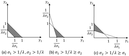
Figure 2: The shaded area in each subfigure presents the set of $(\gamma_{1},\gamma_{2})$ considered in Theorem 1.

IV-B Conditions for No Stable Co-Existence Equilibrium

Theorem 3.

Consider a connected social network with an arbitrary topology, with $\lambda$ denoting the largest eigenvalue of the adjacency matrix. For the privacy-aware $SI_{1}I_{2}S$ problem with a privacy scheme $\begin{bmatrix}r_{11}&r_{12}&1-r_{11}-r_{12}\\ r_{21}&r_{22}&1-r_{21}-r_{22}\end{bmatrix}$, if

$$\frac{1}{2}\left[\begin{array}[]{l}\sigma_{1}r_{11}+\sigma_{2}r_{22}\\[2.0pt] +\sqrt{(\sigma_{1}r_{11}-\sigma_{2}r_{22})^{2}+4\sigma_{1}\sigma_{2}r_{12}r_{21}}\end{array}\right]<\frac{1}{\lambda},$$ (18)

the system will reach a stable equilibrium where both products die out (more specifically, the probability of any user adopting any product is zero in the stable equilibrium).

We explain the basic ideas and the corresponding challenges to establish Theorem 3 in Section VI-C on Page VI-C. The proof details are given in Appendix C-B on Page C-B. Theorem 3 further implies Remark 4 below.

Remark 4.

If $\sigma_{1}<1/\lambda$ and $\sigma_{2}<1/\lambda$, any privacy scheme $\begin{bmatrix}r_{11}&r_{12}&1-r_{11}-r_{12}\\ r_{21}&r_{22}&1-r_{21}-r_{22}\end{bmatrix}$ satisfies (18). Then Theorem 3 implies that if $\sigma_{1}<1/\lambda$ and $\sigma_{2}<1/\lambda$, both products always die out under any privacy scheme.

Remark 4 will be proved in Appendix C-A.

Remark 5.

Given (14), we use Theorem 3 to obtain Remark 1; i.e., under a perfect privacy scheme $\begin{bmatrix}\gamma_{1}&\gamma_{2}&1-\gamma_{1}-\gamma_{2}\\ \gamma_{1}&\gamma_{2}&1-\gamma_{1}-\gamma_{2}\end{bmatrix}$, if $\sigma_{1}\gamma_{1}+\sigma_{2}\gamma_{2}<1/\lambda$, the system will reach a stable equilibrium where both products die out.

V Experiments

To confirm our analytical results in Section IV, we perform experiments on social networks and plot a few figures.

For a comprehensive study, we consider networks of different scales: a small-scale social network called HumanSocial, a large-scale physical contact network called PhysicalContact, and a vast-scale Google+ network [35]. The HumanSocial and PhysicalContact networks are “physical” social networks, while the Google+ network is an online social network. The HumanSocial network from the Koblenz Network Collection has 2,539 nodes and 12,969 edges, where nodes represent students, and an edge between two nodes means that one node is among the other node’s 5 best female friends or 5 best male friends (we remove directions in edges of the original network). The PhysicalContact network [36] represents a synthetic population of the city of Portland, Oregon, USA, and contains about 31 millions links (interactions) among about 1.6 millions nodes (people). The Google+ network [35], crawled from July 2011 to October 2011, consists of 28,942,911 users and 947,776,172 edges.

In Figures LABEL:diffusion1 (a)–(d), we perform experiments on the HumanSocial network. The abbreviation “CD” on the top of figures is short for competitive diffusion, and $\lambda$ denotes the largest eigenvalue of the adjacency matrix of the network. In Figure LABEL:diffusion1a (resp., LABEL:diffusion1b), we consider privacy-aware (resp., privacy-oblivious) competitive diffusion, and set $\sigma_{1}$ and $\sigma_{2}$ both greater than $1/\lambda$ (i.e., the epidemic threshold for single-product diffusion). In Figure LABEL:diffusion1c (resp., LABEL:diffusion1d), we look at privacy-aware (resp., privacy-oblivious) competitive diffusion and consider $\sigma_{1}>1/\lambda>\sigma_{2}$. For privacy-aware competitive diffusion in Figures LABEL:diffusion1a and LABEL:diffusion1c, we observe the co-existence of products in the equilibrium where the number of adopted users for each product is positive. For privacy-oblivious competitive diffusion in Figures LABEL:diffusion1b and LABEL:diffusion1d, we see that the product with weaker strength will die out. We also note that for the initial numbers of adopted users, we select the same combinations across some figures and different combinations across some other figures for a comprehensive comparison. In Figures LABEL:diffusion2 (a)–(d) and LABEL:PhysicalContact (a)–(d), we perform experiments on the large-scale Google+ network and PhysicalContact network. The explanations of Figures LABEL:diffusion2 (a)–(d) and LABEL:PhysicalContact (a)–(d) are similar to those of Figures LABEL:diffusion1 (a)–(d), and we do not repeat them here.

Figures LABEL:diffusion1–LABEL:PhysicalContact (a)–(d) support Theorem 1 and its Remark 3. We further use Figures LABEL:diffusion5 (a)–(f) to confirm Theorem 3 and its Remark 4, where we show that if $\sigma_{1}<1/\lambda$ and $\sigma_{2}<1/\lambda$, then no privacy scheme $\begin{bmatrix}r_{11}&r_{12}&1-r_{11}-r_{12}\\ r_{21}&r_{22}&1-r_{21}-r_{22}\end{bmatrix}$ induces the co-existence of products in the equilibrium. We consider privacy-aware competitive diffusion in all of Figures LABEL:diffusion5 (a)–(f). Figures LABEL:diffusion5a and LABEL:diffusion5b are for the HumanSocial network; Figures LABEL:diffusion5c and LABEL:diffusion5d are for the Google+ network; Figures LABEL:diffusion5e and LABEL:diffusion5f are for the PhysicalContact network. As we can see, both products become extinct in Figures LABEL:diffusion5 (a)–(d). This is in consistence with Theorem 3 and its Remark 4.

Theorem 2 considers complete graphs, so we plot Figures LABEL:completegraph-coexist and LABEL:completegraph-no-coexist for complete graphs. We consider the case of $\sigma_{1}>1/\lambda$ and $\sigma_{2}>1/\lambda$ in Figures LABEL:completegraph-coexist (a) and (b), consider $\sigma_{1}>1/\lambda>\sigma_{2}$ in Figures LABEL:completegraph-coexist (c) and (d), and consider $\sigma_{1}<1/\lambda$ and $\sigma_{2}<1/\lambda$ in Figure LABEL:completegraph-no-coexist ($\lambda$ equals $n-1$ for complete graphs of $n$ nodes, as explained in Footnote 5). For privacy-aware competitive diffusion in Figures LABEL:completegraph-coexist1 and LABEL:completegraph-coexist3, we observe the co-existence of products in the equilibrium where the number of adopted users for each product is positive. For privacy-oblivious competitive diffusion in Figures LABEL:completegraph-coexist2 and LABEL:completegraph-coexist4, the product with weaker strength will die out. Hence, Figures LABEL:completegraph-coexist (a)–(d) and LABEL:completegraph-no-coexist (a)–(b) all confirm Theorem 2.

Summarizing the above, the experiments have confirmed our theoretical results in Section IV.

VI Proof Sketches of Theorem 1–3

In this section, we sketch the proofs for establishing Theorem 1–3 of Section IV.

VI-A Basic Proof Ideas

As discussed in the “Technical approach” paragraph on Page 1, the proofs consist of the following steps:

• Dynamical System. We build a dynamical system of differential equations to describe the privacy-aware competitive diffusion problem.

• Finding Equilibria. Based on the dynamical system, we find all possible equilibria.

• Stability of Equilibria. We analyze whether each equilibrium is stable (i.e., attracting).

We now elaborate the above three steps respectively.

Dynamical System. We construct a dynamical system of differential equations to describe the privacy-aware competitive diffusion problem $S{I_{1}}{I_{2}}S$ with a privacy scheme $\begin{bmatrix}r_{11}&r_{12}&1-r_{11}-r_{12}\\ r_{21}&r_{22}&1-r_{21}-r_{22}\end{bmatrix}$.

Let $A$ be the adjacency matrix of the social network of $n$ users (i.e., nodes) numbered from $1$ to $n$. Then $a_{ij}$ denotes the entry in the $i$th row and the $j$the entry of $A$: $a_{ij}=1$ if there is a link between users $i$ and $j$, and $a_{ij}=0$ otherwise (we set $a_{ii}=0$ so there are no self-links). We consider undirected networks so $A$ is symmetric. For $i=1,2,\ldots,n$, let $p_{i,1}$ denote the probability of node $i$ being in the $I_{1}$ state (i.e., using product 1). Similarly, we define $p_{i,2}$ as the probability of node $i$ being in the $I_{2}$ state (i.e., using product 2), and define $s_{i}$ as the probability of node $i$ being in the $S$ state (i.e., healthy). Clearly, $s_{i}=1-p_{i,1}-p_{i,2}$.

For product $1$, its spreading has two different kinds of sources: 1) users adopting product $1$ honestly spread product $1$ (for each user, this happens with probability $r_{11}$); and 2) users adopting product $2$ pretend using product $1$ and disseminate product $1$ (for each user, this happens with probability $r_{21}$). Hence, for each user $i$, another user $j$ contributes to $i$’s adoption of product $1$ with a rate of $\beta_{1}\big{[}a_{ij}(r_{11}p_{j,1}+r_{21}p_{j,2})\big{]}$, where $a_{ij}$ is multiplied so that the contribution is non-zero only if $j$ is $i$’s neighbor in the network, and $\beta_{1}$ is multiplied since it is the infection rate of product $1$. Then we take a summation for $j$ from $1$ to $n$ and have $\beta_{1}\sum_{j=1}^{n}\big{[}a_{ij}(r_{11}p_{j,1}+r_{21}p_{j,2})\big{]}$ (note that $a_{ij}=1$ for neighboring nodes $i$ and $j$, $a_{ij}=0$ for non-neighboring nodes $i$ and $j$, and also $a_{ii}=0$ so this summation essentially considers only $i$’s neighbors). We further multiply this summation with $s_{i}$ (the probability that node $i$ is susceptible) to obtain the rate that contributes to the increase of $p_{i,1}$ (i.e., the probability that node $i$ adopts product $1$) over time. On the other hand, since the healing rate of product $1$ is $\delta_{1}$, we multiply $\delta_{1}$ with $p_{i,1}$ to obtain the rate that contributes to the decrease of $p_{i,1}$ over time. Given these, we finally obtain that $\frac{\textrm{d}\hskip 1.0ptp_{i,1}}{\textrm{d}\hskip 1.0ptt}$ is the result of the rate $\beta_{1}s_{i}\bigg{\{}\sum_{j=1}^{n}\big{[}a_{ij}(r_{11}p_{j,1}+r_{21}p_{j,2})\big{]}\bigg{\}}$ minus the rate $\delta_{1}p_{i,1}$; i.e., we have (19b) below. Similarly, by analyzing the change of $p_{i,2}$ (i.e., the probability that node $i$ adopts product $2$) over time, we obtain (19d) below. Hence, the dynamical system characterizing our privacy-aware $SI_{1}I_{2}S$ competitive diffusion is given by

$$\frac{\textrm{d}\hskip 1.0ptp_{i,1}}{\textrm{d}\hskip 1.0ptt}$$ (19a)

$$=-\delta_{1}p_{i,1}+\beta_{1}s_{i}\bigg{\{}\sum_{j=1}^{n}\big{[}a_{ij}(r_{11}p_{j,1}+r_{21}p_{j,2})\big{]}\bigg{\}},$$ (19b)

$$\frac{\textrm{d}\hskip 1.0ptp_{i,2}}{\textrm{d}\hskip 1.0ptt}$$ (19c)

$$=-\delta_{2}p_{i,2}+\beta_{2}s_{i}\bigg{\{}\sum_{j=1}^{n}\big{[}a_{ij}(r_{12}p_{j,1}+r_{22}p_{j,2})\big{]}\bigg{\}}.$$ (19d)

Equilibria. With the dynamical system given above, it is straightforward to characterize possible equilibria.

At an equilibrium, $\frac{\textrm{d}\hskip 1.0ptp_{i,1}}{\textrm{d}\hskip 1.0ptt}=0$ and $\frac{\textrm{d}\hskip 1.0ptp_{i,2}}{\textrm{d}\hskip 1.0ptt}=0$ hold. Applying these to (19b) and (19d), and recalling $\sigma_{1}\stackrel{{\scriptstyle\text{def}}}{{=}}\beta_{1}/\delta_{1}$ and $\sigma_{2}\stackrel{{\scriptstyle\text{def}}}{{=}}\beta_{2}/\delta_{2}$, we obtain

$${p}_{i,1} =\sigma_{1}{s}_{i}\bigg{\{}\sum_{j=1}^{n}\big{[}a_{ij}(r_{11}{p}_{j,1}+r_{21}{p}_{j,2})\big{]}\bigg{\}},$$ (20)

and

$${p}_{i,2} =\sigma_{2}{s}_{i}\bigg{\{}\sum_{j=1}^{n}\big{[}a_{ij}(r_{12}{p}_{j,1}+r_{22}{p}_{j,2})\big{]}\bigg{\}}.$$ (21)

To write (20) and (21) conveniently in the vector/matrix form, we let ${\mbox{\boldmath{$P$}}}_{1}$ (resp., ${\mbox{\boldmath{$P$}}}_{2}$) be the column vector $[{p}_{1,1},{p}_{2,1},\ldots,{p}_{n,1}]^{T}$ (resp., $[{p}_{1,2},{p}_{2,2},\ldots,{p}_{n,2}]^{T}$), where “^T” means “transpose”; i.e., the vector ${\mbox{\boldmath{$P$}}}_{1}$ (resp., ${\mbox{\boldmath{$P$}}}_{2}$) contains the probability of each user adopting product 1 (resp., product 2). We also define $S$ as the column vector $[s_{1},s_{2},\ldots,s_{n}]^{T}$; i.e., the vector $S$ contains the probability of each user not adopting any product.

Writing (20) and (21) in the vector/matrix form, we have

$${\mbox{\boldmath{$P$}}}_{1} =\sigma_{1}{\mbox{\boldmath{${S}$}}}{\mbox{\boldmath{$A$}}}(r_{11}{\mbox{\boldmath{${P}$}}}_{1}+r_{21}{\mbox{\boldmath{${P}$}}}_{2}),$$ (22)

and

$${\mbox{\boldmath{$P$}}}_{2} =\sigma_{2}{\mbox{\boldmath{${S}$}}}{\mbox{\boldmath{$A$}}}(r_{12}{\mbox{\boldmath{${P}$}}}_{1}+r_{22}{\mbox{\boldmath{${P}$}}}_{2}).$$ (23)

VI-B Ideas and Challenges to Establish Theorems 1 and 2

From the statements of Theorem 1 and 2 on Page 1 and the proof ideas in Section VI-A, we will find all equilibria and show that the system has only one stable equilibrium. In this equilibrium, both products co-exist; namely, all elements of ${\mbox{\boldmath{$P$}}}_{1}$ and ${\mbox{\boldmath{$P$}}}_{2}$ are positive (i.e., greater than $0$). Compared with finding the equilibrium points, proving the stability of the co-existence equilibrium is more challenging here. From stability theory, we will show that all eigenvalues of the corresponding Jacobian matrix have negative real parts. Due to the introduction of privacy, the dynamics for the two products are coupled together, so the Jacobian matrix is dense in the sense that most (or even all) entries are non-zero. This makes it significantly challenging to analyze the Jacobian matrix’s eigenvalues.

VI-C Ideas and Challenges to Establish Theorem 3

From the statement of Theorem 3, our goal is to show that the system has only one stable equilibrium, which turns out to be a zero equilibrium; i.e., all elements of ${\mbox{\boldmath{$P$}}}_{1}$ and ${\mbox{\boldmath{$P$}}}_{2}$ are zero in this equilibrium. The idea here is to connect our equilibrium with the equilibrium of an $SIS$ diffusion problem, and prove the former equilibrium being zero by first showing the latter equilibrium being zero. The challenging part is to connect our privacy-aware $SI_{1}I_{2}S$ diffusion problem with an $SIS$ diffusion problem, since the privacy scheme considered in Theorem 3 is very general.

VII Conclusion

In competitive diffusion where two products compete for user adoption, prior studies show that the weaker product will soon become extinct. However, in practice, competing products often co-exist in the market. We find that considering user privacy can address this discrepancy. More specifically, we incorporate user privacy into competitive diffusion to propose the novel problem of privacy-aware competitive diffusion, and formally show that privacy can enable the co-existence of competing products.

Appendix A Useful Lemmas

To establish our main results, we find it useful to present Lemmas 1–3 below. These lemmas apply for a privacy-aware $SI_{1}I_{2}S$ problem with a privacy scheme $\begin{bmatrix}r_{11}&r_{12}&1-r_{11}-r_{12}\\ r_{21}&r_{22}&1-r_{21}-r_{22}\end{bmatrix}$ satisfying $\begin{Bmatrix}0<r_{11}<1,~{}~{}&~{}~{}0<r_{12}<1,\\ 0<r_{21}<1,~{}~{}&~{}~{}0<r_{22}<1,\\ r_{11}+r_{12}\leq 1,~{}~{}&~{}~{}r_{21}+r_{22}\leq 1.\end{Bmatrix}$. The proofs of Lemmas 1–3 are presented in Appendix A of the online full version [34], due to space limitation.

Lemma 1.

At an equilibrium, we have $s_{i}\neq 0$ for any $i=1,2,\ldots,n$.

Lemma 2.

At an equilibrium, we have

• $p_{i,1}=0$ and $p_{i,2}=0$ for $i=1,2,\ldots,n$ such that ${\mbox{\boldmath{$P$}}}_{1}={\mbox{\boldmath{$0$}}}$ and ${\mbox{\boldmath{$P$}}}_{2}={\mbox{\boldmath{$0$}}}$,

• $p_{i,1}>0$ and $p_{i,2}>0$ for $i=1,2,\ldots,n$ such that ${\mbox{\boldmath{$P$}}}_{1}$ and ${\mbox{\boldmath{$P$}}}_{2}$ are both positive vectors (a positive vector means that each dimension is positive).

Lemma 3.

At an equilibrium, we have the following properties for the matrix ${S}$$A$.

• ${S}$$A$ is non-negative and irreducible.

• ${S}$$A$ has a unique positive real number (say $\lambda({\mbox{\boldmath{${S}$}}}{\mbox{\boldmath{$A$}}})$) as its largest eigenvalue (in magnitude). Furthermore, the algebraic multiplicity of $\lambda({\mbox{\boldmath{${S}$}}}{\mbox{\boldmath{$A$}}})$ is 1, and it has a positive eigenvector.

• Except the largest eigenvalue $\lambda({\mbox{\boldmath{${S}$}}}{\mbox{\boldmath{$A$}}})$, no other eigenvalue of ${S}$$A$ has a positive eigenvector.

Appendix B Proving Theorem 1 and its Remark 3

This section is organized as follows. We prove Remark 3 of Theorem 1 in Appendix B-A, and establish Theorem 1 in Appendix B-B.

B-A Proving Remark 3 of Theorem 1

The proof of Remark 3 is straightforward and is still presented here for clarity. We discuss the three cases of Remark 3.

• Under $\sigma_{1}>1/\lambda$ and $\sigma_{2}>1/\lambda$, we will show that

  $$\begin{Bmatrix}\text{(i): }\sigma_{1}\gamma_{1}+\sigma_{2}\gamma_{2}>1/\lambda,\\ \text{(ii): }0<\gamma_{1}<1,~{}~{}\text{(iii): }0<\gamma_{2}<1,~{}~{}\text{(iv): }\gamma_{1}+\gamma_{2}\leq 1.\end{Bmatrix}$$ (24)

  is equivalent to

  $$\begin{Bmatrix}\text{(i): }0<\gamma_{1}<1,\\ \text{(ii): }\max\big{\{}0,\frac{\lambda^{-1}-\sigma_{1}\gamma_{1}}{\sigma_{2}}\big{\}}<\gamma_{2}\leq 1-\gamma_{1}.\end{Bmatrix}$$ (25)

  To see (25) $\Longrightarrow$ (24), we obtain (24)-(i) from $\gamma_{2}>\frac{\lambda^{-1}-\sigma_{1}\gamma_{1}}{\sigma_{2}}$ of (25)-(ii), while the inequalities (ii) (iii) (iv) in the second row of (24) follow clearly from (25). To see (24) $\Longrightarrow$ (25), we have (25)-(i) from (24)-(ii) and obtain (25)-(ii) from (24)-(i) (iii) (iv).

• Under $\sigma_{1}>1/\lambda\geq\sigma_{2}$, we will show that (24) is equivalent to

  $$\begin{Bmatrix}\text{(i): }\frac{\lambda^{-1}-\sigma_{2}}{\sigma_{1}-\sigma_{2}}<\gamma_{1}<1,\\ \text{(ii): }\max\big{\{}0,\frac{\lambda^{-1}-\sigma_{1}\gamma_{1}}{\sigma_{2}}\big{\}}<\gamma_{2}\leq 1-\gamma_{1}.\end{Bmatrix}.$$ (26)

  To see (26) $\Longrightarrow$ (24), we obtain (24)-(i) from $\gamma_{2}>\frac{\lambda^{-1}-\sigma_{1}\gamma_{1}}{\sigma_{2}}$ of (26)-(ii), obtain (24)-(ii) from (26)-(i) and the condition $1/\lambda\geq\sigma_{2}$ here, obtain (24)-(iii) from (26)-(ii) and the just-proved result $\gamma_{1}>0$ of (24)-(ii), and obtain (24)-(iv) from (26)-(ii). To see (24) $\Longrightarrow$ (26), we obtain (26)-(i) from (24)-(i) (ii) (iv), obtain (26)-(ii) from (24)-(i) (iii) (iv).

• Under $\sigma_{2}>1/\lambda\geq\sigma_{1}$, we will show that (15) is equivalent to

  $$\begin{Bmatrix}\text{(i): }0<\gamma_{1}<\frac{\sigma_{2}-\lambda^{-1}}{\sigma_{2}-\sigma_{1}},\\ \text{(ii): }\frac{\lambda^{-1}-\sigma_{1}\gamma_{1}}{\sigma_{2}}<\gamma_{2}\leq 1-\gamma_{1}.\end{Bmatrix}.$$ (27)

  To see (27) $\Longrightarrow$ (24), we obtain (24)-(i) from $\gamma_{2}>\frac{\lambda^{-1}-\sigma_{1}\gamma_{1}}{\sigma_{2}}$ of (27)-(ii), obtain (24)-(ii) from (27)-(i) and the condition $1/\lambda\geq\sigma_{1}$ here, obtain (24)-(iii) from (27)-(ii), the condition $1/\lambda\geq\sigma_{1}$ here and the just-proved result $0<\gamma_{1}<1$ of (24)-(ii), and obtain (24)-(iv) from (27)-(ii). To see (24) $\Longrightarrow$ (27), we obtain (27)-(i) from (24)-(i) (ii) (iv), obtain (27)-(ii) from (24)-(i) (iii) (iv).

B-B Proof of Theorem 1

We now prove Theorem 1 in detail. Specifically, based on (19b) and (19d), we will discuss equilibrium points in Appendix B-B1 and their stability in Appendix B-B2. Although Theorem 1 considers privacy schemes in the form of $\begin{bmatrix}\gamma_{1}&\gamma_{2}&1-\gamma_{1}-\gamma_{2}\\ \gamma_{1}&\gamma_{2}&1-\gamma_{1}-\gamma_{2}\end{bmatrix}$, we will often use a general privacy scheme $\begin{bmatrix}r_{11}&r_{12}&1-r_{11}-r_{12}\\ r_{21}&r_{22}&1-r_{21}-r_{22}\end{bmatrix}$ to present a general analysis, which will be useful later for proving other theorems.

B-B1 Equilibrium points

From Lemma 2, an equilibrium

• either satisfies $p_{i,1}=0$ and $p_{i,2}=0$ for $i=1,2,\ldots,n$ such that ${\mbox{\boldmath{$P$}}}_{1}={\mbox{\boldmath{$0$}}}$ and ${\mbox{\boldmath{$P$}}}_{2}={\mbox{\boldmath{$0$}}}$,

• or satisfies $p_{i,1}>0$ and $p_{i,2}>0$ for $i=1,2,\ldots,n$ such that ${\mbox{\boldmath{$P$}}}_{1}$ and ${\mbox{\boldmath{$P$}}}_{2}$ are both positive vectors (a positive vector means that each dimension is positive).

We further analyze the second case below.

Computing $\textrm{(\ref{dp1idt-equilibrium-matrix})}\times\sigma_{2}r_{22}-\textrm{(\ref{dp2idt-equilibrium-matrix})}\times\sigma_{1}r_{21}$, we have

$$\sigma_{2}r_{22}{\mbox{\boldmath{$P$}}}_{1}-\sigma_{1}r_{21}{\mbox{\boldmath{$P$}}}_{2}=\sigma_{1}\sigma_{2}(r_{11}r_{22}-r_{12}r_{21}){\mbox{\boldmath{$S$}}}{\mbox{\boldmath{$A$}}}{\mbox{\boldmath{$P$}}}_{1}.$$ (28)

Computing $\textrm{(\ref{dp1idt-equilibrium-matrix})}\times\sigma_{2}r_{12}-\textrm{(\ref{dp2idt-equilibrium-matrix})}\times\sigma_{1}r_{11}$, we have

$$\sigma_{2}r_{12}{\mbox{\boldmath{$P$}}}_{1}-\sigma_{1}r_{11}{\mbox{\boldmath{$P$}}}_{2}=\sigma_{1}\sigma_{2}(r_{12}r_{21}-r_{11}r_{22}){\mbox{\boldmath{$S$}}}{\mbox{\boldmath{$A$}}}{\mbox{\boldmath{$P$}}}_{2}.$$ (29)

Under $r_{11}r_{22}=r_{12}r_{21}$ (which clearly holds given $r_{11}=r_{21}=\gamma_{1}$ and $r_{12}=r_{22}=\gamma_{2}$ for the privacy scheme $\begin{bmatrix}\gamma_{1}&\gamma_{2}&1-\gamma_{1}-\gamma_{2}\\ \gamma_{1}&\gamma_{2}&1-\gamma_{1}-\gamma_{2}\end{bmatrix}$ considered in Theorem 1 here), we obtain from (28) (resp., (29)) that

$$\textstyle{{\mbox{\boldmath{$P$}}}_{1}=\frac{\sigma_{1}r_{21}}{\sigma_{2}r_{22}}{\mbox{\boldmath{$P$}}}_{2}\text{ (resp., }{\mbox{\boldmath{$P$}}}_{1}=\frac{\sigma_{1}r_{11}}{\sigma_{2}r_{12}}{\mbox{\boldmath{$P$}}}_{2}\text{)}}.$$ (30)

The above two results ${\mbox{\boldmath{$P$}}}_{1}=\frac{\sigma_{1}r_{21}}{\sigma_{2}r_{22}}{\mbox{\boldmath{$P$}}}_{2}$ and ${\mbox{\boldmath{$P$}}}_{1}=\frac{\sigma_{1}r_{11}}{\sigma_{2}r_{12}}{\mbox{\boldmath{$P$}}}_{2}$ are the same given $r_{11}r_{22}=r_{12}r_{21}$. Substituting ${\mbox{\boldmath{$P$}}}_{1}=\frac{\sigma_{1}r_{21}}{\sigma_{2}r_{22}}{\mbox{\boldmath{$P$}}}_{2}$ into (22), we obtain

$${\mbox{\boldmath{$P$}}}_{\ell} =(\sigma_{1}r_{11}+\sigma_{2}r_{22}){\mbox{\boldmath{${S}$}}}{\mbox{\boldmath{$A$}}}{\mbox{\boldmath{$P$}}}_{\ell},\text{ for }\ell=1,2.$$ (31)

With $Q$ denoting ${\mbox{\boldmath{$P$}}}_{1}+{\mbox{\boldmath{$P$}}}_{2}$, (31) implies

$$Q =(\sigma_{1}r_{11}+\sigma_{2}r_{22}){\mbox{\boldmath{${S}$}}}{\mbox{\boldmath{$A$}}}{\mbox{\boldmath{$Q$}}}.$$ (32)

From (32), as will be clear soon, it is useful to look at a traditional privacy-oblivious $SIS$ diffusion problem (not our privacy-aware $SI_{1}I_{2}S$ competitive diffusion problem, yet still on the network with adjacency matrix $A$) with infection rate $\beta_{*}$ and healing rate $\delta_{*}$ satisfying

$$\textstyle{\beta_{*}/\delta_{*}=\sigma_{1}r_{11}+\sigma_{2}r_{22}.}$$ (33)

For $i=1,2,\ldots,n$, with $q_{i}$ denoting the probability of node $i$ being infected in the above $SIS$ diffusion problem, it is well-known that the dynamical system characterizing $SIS$ diffusion is given by

$$\frac{\textrm{d}\hskip 1.0ptq_{i}}{\textrm{d}\hskip 1.0ptt} =-\delta_{*}q_{i}+\beta_{*}(1-q_{i})\sum_{j=1}^{n}(a_{ij}q_{j}).$$ (34)

Below we explain (34) for the above $SIS$ diffusion problem. For each user $i$, another user $j$ contributes to $i$’s infection with a rate of $\beta_{*}a_{ij}q_{j}$, where $a_{ij}$ is multiplied so that the contribution is non-zero only if $j$ is $i$’s neighbor in the network, and $\beta_{*}$ is multiplied since it is the infection rate. Then we take a summation for $j$ from $1$ to $n$ and have $\beta_{*}\sum_{j=1}^{n}(a_{ij}q_{j})$ (note that $a_{ij}=1$ for neighboring nodes $i$ and $j$, $a_{ij}=0$ for non-neighboring nodes $i$ and $j$, and also $a_{ii}=0$ so this summation essentially considers only $i$’s neighbors). We further multiply this summation with $1-q_{i}$ (the probability that node $i$ is susceptible) to obtain the rate that contributes to the increase of $q_{i}$ over time. On the other hand, since the healing rate is $\delta_{*}$, we multiply $\delta_{*}$ with $q_{i}$ to obtain the rate that contributes to the decrease of $q_{i}$ over time. Given these, we obtain that $\frac{\textrm{d}\hskip 1.0ptq_{i}}{\textrm{d}\hskip 1.0ptt}$ is the result of the rate $\beta_{*}(1-q_{i})\sum_{j=1}^{n}(a_{ij}q_{j})$ minus the rate $\delta_{*}q_{i}$; i.e., we have (34).

In the above $SIS$ problem, at an equilibrium, (33) (34) and $\frac{\textrm{d}\hskip 1.0ptq_{i}}{\textrm{d}\hskip 1.0ptt}=0$ together imply

$$q_{i}=(\sigma_{1}r_{11}+\sigma_{2}r_{22})(1-q_{i})\sum_{j=1}^{n}(a_{ij}q_{j}).$$ (35)

We recall (32), where $Q$ is a column vector with elements $p_{i,1}+p_{i,2}$ for $i=1,2,\ldots,n$, and $S$ is a diagonal matrix with elements $1-(p_{i,1}+p_{i,2})$ for $i=1,2,\ldots,n$. This and (35) together mean that $p_{i,1}+p_{i,2}$ can be understood as $q_{i}$ in (35) for $i=1,2,\ldots,n$ so that $Q$ is an equilibrium of the above $SIS$ problem. As shown in prior work [15, 16, 17], with $\lambda$ denoting the largest eigenvalue of the adjacency matrix $A$, for the above $SIS$ problem, on the one hand, if $\beta_{*}/\delta_{*}<1/\lambda$, the only equilibrium is ${\mbox{\boldmath{$Q$}}}={\mbox{\boldmath{$0$}}}$, which implies ${\mbox{\boldmath{$P$}}}_{1}={\mbox{\boldmath{$0$}}}$ and ${\mbox{\boldmath{$P$}}}_{2}={\mbox{\boldmath{$0$}}}$ from ${\mbox{\boldmath{$Q$}}}={\mbox{\boldmath{$P$}}}_{1}+{\mbox{\boldmath{$P$}}}_{2}$ and ${\mbox{\boldmath{$P$}}}_{1}=\frac{\sigma_{1}r_{21}}{\sigma_{2}r_{22}}{\mbox{\boldmath{$P$}}}_{2}$; on the other hand, if

$$\beta_{*}/\delta_{*}>1/\lambda,$$ (36)

an equilibrium of positive $Q$ exists and can be determined by $A$ and $\beta_{*}/\delta_{*}$. We denote this equilibrium by ${\mbox{\boldmath{$V$}}}_{\text{SIS}}({\mbox{\boldmath{$A$}}},\beta_{*}/\delta_{*})$. Then if

$$\sigma_{1}r_{11}+\sigma_{2}r_{22}>1/\lambda$$ (37)

which holds from (33) and (36), we use ${\mbox{\boldmath{$P$}}}_{1}=\frac{\sigma_{1}r_{21}}{\sigma_{2}r_{22}}{\mbox{\boldmath{$P$}}}_{2}$, ${\mbox{\boldmath{$Q$}}}={\mbox{\boldmath{$P$}}}_{1}+{\mbox{\boldmath{$P$}}}_{2}$, and ${\mbox{\boldmath{$Q$}}}={\mbox{\boldmath{$V$}}}_{\text{SIS}}({\mbox{\boldmath{$A$}}},\beta_{*}/\delta_{*})$ to obtain an equilibrium of positive vectors ${\mbox{\boldmath{$P$}}}_{1}$ and ${\mbox{\boldmath{$P$}}}_{2}$:

$${\mbox{\boldmath{$P$}}}_{1} =\frac{\sigma_{1}r_{21}}{\sigma_{1}r_{21}+\sigma_{2}r_{22}}\cdot{\mbox{\boldmath{$V$}}}_{\text{SIS}}({\mbox{\boldmath{$A$}}},\beta_{*}/\delta_{*}),$$ (38)

$${\mbox{\boldmath{$P$}}}_{2} =\frac{\sigma_{2}r_{22}}{\sigma_{1}r_{21}+\sigma_{2}r_{22}}\cdot{\mbox{\boldmath{$V$}}}_{\text{SIS}}({\mbox{\boldmath{$A$}}},\beta_{*}/\delta_{*}).$$ (39)

To summarize, under $r_{11}=r_{21}=\gamma_{1}$, $r_{12}=r_{22}=\gamma_{2}$ and (37), we have the following.

• An equilibrium of positive ${\mbox{\boldmath{$P$}}}_{1}$ and ${\mbox{\boldmath{$P$}}}_{2}$ is given by (38) and (39). In Appendix B-B2 below, we will show that this equilibrium is stable under (37).

• Another equilibrium is the zero equilibrium: ${\mbox{\boldmath{$P$}}}_{1}={\mbox{\boldmath{$0$}}}$ and ${\mbox{\boldmath{$P$}}}_{2}={\mbox{\boldmath{$0$}}}$. In Appendix B-B3 below, we will show that this equilibrium is unstable under (37).

B-B2 Stability of the equilibrium given by (38) and (39)

To prove Theorem 1, we will show that the equilibrium of positive ${\mbox{\boldmath{$P$}}}_{1}$ and ${\mbox{\boldmath{$P$}}}_{2}$ given by (38) and (39) is stable given $r_{11}=r_{21}$, $r_{12}=r_{22}$, and (37). To this end, we will derive the Jacobian matrix based on (20) and (21), and prove that all of its eigenvalues have negative real parts.

The Jacobian matrix has four parts $\begin{bmatrix}{\mbox{\boldmath{$J$}}}_{11}&{\mbox{\boldmath{$J$}}}_{12}\\ {\mbox{\boldmath{$J$}}}_{21}&{\mbox{\boldmath{$J$}}}_{22}\end{bmatrix}$, where each ${\mbox{\boldmath{$J$}}}_{ab}$ for row index $a=1,2$ and column index $b=1,2$ is an $n\times n$ matrix comprising $\frac{1}{\partial p_{j,b}}\partial\frac{\textrm{d}\hskip 1.0ptp_{i,a}}{\textrm{d}\hskip 1.0ptt}$ for row index $i=1,2,\ldots,n$ and column index $j=1,2,\ldots,n$. In other words,

• $\frac{1}{\partial p_{j,1}}\partial\frac{\textrm{d}\hskip 1.0ptp_{i,1}}{\textrm{d}\hskip 1.0ptt}$ is in the $i$th row and $j$th column of ${\mbox{\boldmath{$J$}}}_{11}$;

• $\frac{1}{\partial p_{j,2}}\partial\frac{\textrm{d}\hskip 1.0ptp_{i,1}}{\textrm{d}\hskip 1.0ptt}$ is in the $i$th row and $j$th column of ${\mbox{\boldmath{$J$}}}_{12}$;

• $\frac{1}{\partial p_{j,1}}\partial\frac{\textrm{d}\hskip 1.0ptp_{i,2}}{\textrm{d}\hskip 1.0ptt}$ is in the $i$th row and $j$th column of ${\mbox{\boldmath{$J$}}}_{21}$;

• $\frac{1}{\partial p_{j,2}}\partial\frac{\textrm{d}\hskip 1.0ptp_{i,2}}{\textrm{d}\hskip 1.0ptt}$ is in the $i$th row and $j$th column of ${\mbox{\boldmath{$J$}}}_{22}$.

To compute the matrix ${\mbox{\boldmath{$J$}}}_{11}$ which contains $\frac{1}{\partial p_{j,1}}\partial\frac{\textrm{d}\hskip 1.0ptp_{i,1}}{\textrm{d}\hskip 1.0ptt}$ for $i=1,2,\ldots,n$ and $j=1,2,\ldots,n$, from (19b) and $s_{i}=1-p_{i,1}-p_{i,2}$, we obtain

$$\frac{1}{\partial p_{i,1}}\partial\frac{\textrm{d}\hskip 1.0ptp_{i,1}}{\textrm{d}\hskip 1.0ptt}$$

$$=-\delta_{1}+\beta_{1}r_{11}\cdot s_{i}a_{ii}$$

$$~{}~{}~{}~{}~{}~{}~{}~{}-\beta_{1}\bigg{[}r_{11}\sum_{j=1}^{n}(a_{ij}p_{j,1})+r_{21}\sum_{j=1}^{n}(a_{ij}p_{j,2})\bigg{]},$$ (40)

and for $j\neq i$,

$$\frac{1}{\partial p_{j,1}}\partial\frac{\textrm{d}\hskip 1.0ptp_{i,1}}{\textrm{d}\hskip 1.0ptt}=\beta_{1}r_{11}\cdot s_{i}a_{ij}.$$ (41)

To express ${\mbox{\boldmath{$J$}}}_{11}$ using (40) and (41), we now introduce some notation. Let $I$ be the $n\times n$ unit matrix. We define an $n\times n$ diagonal matrix $\textrm{diag}({\mbox{\boldmath{$A$}}}{\mbox{\boldmath{$P$}}}_{1})$ as follows: if ${\mbox{\boldmath{$A$}}}{\mbox{\boldmath{$P$}}}_{1}=[w_{1},w_{2},\ldots,w_{n}]^{T}$, then $\textrm{diag}({\mbox{\boldmath{$A$}}}{\mbox{\boldmath{$P$}}}_{1})$ is the diagonal matrix with elements $w_{1},w_{2},\ldots,w_{n}$ (from the upper left to the lower right). Similarly, we also define an $n\times n$ diagonal matrix $\textrm{diag}({\mbox{\boldmath{$A$}}}{\mbox{\boldmath{$P$}}}_{2})$. With the above notation, we use (40) and (41) to express the matrix ${\mbox{\boldmath{$J$}}}_{11}$ comprising $\frac{1}{\partial p_{j,1}}\partial\frac{\textrm{d}\hskip 1.0ptp_{i,1}}{\textrm{d}\hskip 1.0ptt}$ for row index $i=1,2,\ldots,n$ and column index $j=1,2,\ldots,n$ as follows:

$${\mbox{\boldmath{$J$}}}_{11}= -\delta_{1}{\mbox{\boldmath{$I$}}}+\beta_{1}r_{11}{\mbox{\boldmath{$S$}}}{\mbox{\boldmath{$A$}}}$$

$$-\beta_{1}r_{11}\textrm{diag}({\mbox{\boldmath{$A$}}}{\mbox{\boldmath{$P$}}}_{1})-\beta_{1}r_{21}\textrm{diag}({\mbox{\boldmath{$A$}}}{\mbox{\boldmath{$P$}}}_{2}).$$ (42)

To compute the matrix ${\mbox{\boldmath{$J$}}}_{12}$ which contains $\frac{1}{\partial p_{j,2}}\partial\frac{\textrm{d}\hskip 1.0ptp_{i,1}}{\textrm{d}\hskip 1.0ptt}$ for $i=1,2,\ldots,n$ and $j=1,2,\ldots,n$, from (19b) and $s_{i}=1-p_{i,1}-p_{i,2}$, we obtain

$$\frac{1}{\partial p_{i,2}}\partial\frac{\textrm{d}\hskip 1.0ptp_{i,1}}{\textrm{d}\hskip 1.0ptt}$$

$$=\beta_{1}r_{21}\cdot s_{i}a_{ii}-\beta_{1}\bigg{[}r_{11}\sum_{j=1}^{n}(a_{ij}p_{j,1})+r_{21}\sum_{j=1}^{n}(a_{ij}p_{j,2})\bigg{]},$$ (43)

and for $j\neq i$,

$$\frac{1}{\partial p_{j,2}}\partial\frac{\textrm{d}\hskip 1.0ptp_{i,1}}{\textrm{d}\hskip 1.0ptt}=\beta_{1}r_{21}\cdot s_{i}a_{ij}.$$ (44)

Combining (43) and (44), we express the matrix ${\mbox{\boldmath{$J$}}}_{12}$ comprising $\frac{1}{\partial p_{j,2}}\partial\frac{\textrm{d}\hskip 1.0ptp_{i,1}}{\textrm{d}\hskip 1.0ptt}$ for row index $i=1,2,\ldots,n$ and column index $j=1,2,\ldots,n$ as follows:

$${\mbox{\boldmath{$J$}}}_{12}=\beta_{1}r_{21}{\mbox{\boldmath{$S$}}}{\mbox{\boldmath{$A$}}}-\beta_{1}r_{11}\textrm{diag}({\mbox{\boldmath{$A$}}}{\mbox{\boldmath{$P$}}}_{1})-\beta_{1}r_{21}\textrm{diag}({\mbox{\boldmath{$A$}}}{\mbox{\boldmath{$P$}}}_{2}).$$ (45)

To compute the matrix ${\mbox{\boldmath{$J$}}}_{21}$ which contains $\frac{1}{\partial p_{j,1}}\partial\frac{\textrm{d}\hskip 1.0ptp_{i,2}}{\textrm{d}\hskip 1.0ptt}$ for $i=1,2,\ldots,n$ and $j=1,2,\ldots,n$, from (19d) and $s_{i}=1-p_{i,1}-p_{i,2}$, we obtain

$$\frac{1}{\partial p_{i,1}}\partial\frac{\textrm{d}\hskip 1.0ptp_{i,2}}{\textrm{d}\hskip 1.0ptt}$$

$$=\beta_{2}r_{12}\cdot s_{i}a_{ii}-\beta_{2}\bigg{[}r_{12}\sum_{j=1}^{n}(a_{ij}p_{j,1})+r_{22}\sum_{j=1}^{n}(a_{ij}p_{j,2})\bigg{]},$$ (46)

and for $j\neq i$,

$$\frac{1}{\partial p_{j,1}}\partial\frac{\textrm{d}\hskip 1.0ptp_{i,2}}{\textrm{d}\hskip 1.0ptt}=\beta_{2}r_{12}\cdot s_{i}a_{ij}.$$ (47)

Combining (46) and (47), we express the matrix ${\mbox{\boldmath{$J$}}}_{21}$ comprising $\frac{1}{\partial p_{j,1}}\partial\frac{\textrm{d}\hskip 1.0ptp_{i,2}}{\textrm{d}\hskip 1.0ptt}$ for row index $i=1,2,\ldots,n$ and column index $j=1,2,\ldots,n$ as follows:

$${\mbox{\boldmath{$J$}}}_{21}=\beta_{2}r_{12}{\mbox{\boldmath{$S$}}}{\mbox{\boldmath{$A$}}}-\beta_{2}r_{12}\textrm{diag}({\mbox{\boldmath{$A$}}}{\mbox{\boldmath{$P$}}}_{1})-\beta_{2}r_{22}\textrm{diag}({\mbox{\boldmath{$A$}}}{\mbox{\boldmath{$P$}}}_{2}).$$ (48)

To compute the matrix ${\mbox{\boldmath{$J$}}}_{22}$ which contains $\frac{1}{\partial p_{j,2}}\partial\frac{\textrm{d}\hskip 1.0ptp_{i,2}}{\textrm{d}\hskip 1.0ptt}$ for $i=1,2,\ldots,n$ and $j=1,2,\ldots,n$, from (19d) and $s_{i}=1-p_{i,1}-p_{i,2}$, we obtain

$$\frac{1}{\partial p_{i,2}}\partial\frac{\textrm{d}\hskip 1.0ptp_{i,2}}{\textrm{d}\hskip 1.0ptt}$$

$$=-\delta_{2}+\beta_{2}r_{22}\cdot s_{i}a_{ii}$$

$$~{}~{}~{}~{}~{}~{}~{}~{}-\beta_{2}\bigg{[}r_{12}\sum_{j=1}^{n}(a_{ij}p_{j,1})+r_{22}\sum_{j=1}^{n}(a_{ij}p_{j,2})\bigg{]},$$ (49)

and for $j\neq i$,

$$\frac{1}{\partial p_{j,2}}\partial\frac{\textrm{d}\hskip 1.0ptp_{i,2}}{\textrm{d}\hskip 1.0ptt}=\beta_{2}r_{22}\cdot s_{i}a_{ij}.$$ (50)

Combining (49) and (50), we express the matrix ${\mbox{\boldmath{$J$}}}_{22}$ comprising $\frac{1}{\partial p_{j,2}}\partial\frac{\textrm{d}\hskip 1.0ptp_{i,2}}{\textrm{d}\hskip 1.0ptt}$ for row index $i=1,2,\ldots,n$ and column index $j=1,2,\ldots,n$ as follows:

$${\mbox{\boldmath{$J$}}}_{22}= -\delta_{2}{\mbox{\boldmath{$I$}}}+\beta_{2}r_{22}{\mbox{\boldmath{$S$}}}{\mbox{\boldmath{$A$}}}$$

$$-\beta_{2}r_{12}\textrm{diag}({\mbox{\boldmath{$A$}}}{\mbox{\boldmath{$P$}}}_{1})-\beta_{2}r_{22}\textrm{diag}({\mbox{\boldmath{$A$}}}{\mbox{\boldmath{$P$}}}_{2}).$$ (51)

Our goal is to show that all eigenvalues of the Jacobian matrix $\begin{bmatrix}{\mbox{\boldmath{$J$}}}_{11}&{\mbox{\boldmath{$J$}}}_{12}\\ {\mbox{\boldmath{$J$}}}_{21}&{\mbox{\boldmath{$J$}}}_{22}\end{bmatrix}$ have negative real parts. By definition, with ${\mbox{\boldmath{$I$}}}_{2n}$ denoting the $2n\times 2n$ unit matrix, $x$ is an eigenvalue of $\begin{bmatrix}{\mbox{\boldmath{$J$}}}_{11}&{\mbox{\boldmath{$J$}}}_{12}\\ {\mbox{\boldmath{$J$}}}_{21}&{\mbox{\boldmath{$J$}}}_{22}\end{bmatrix}$ if $\left|\begin{bmatrix}{\mbox{\boldmath{$J$}}}_{11}&{\mbox{\boldmath{$J$}}}_{12}\\ {\mbox{\boldmath{$J$}}}_{21}&{\mbox{\boldmath{$J$}}}_{22}\end{bmatrix}-x{\mbox{\boldmath{$I$}}}_{2n}\right|=0$, where $|\cdot|$ denotes the determinant. From (42) (45) (48) (51), $r_{11}=r_{21}$ and $r_{12}=r_{22}$, it follows that

$$\begin{bmatrix}{\mbox{\boldmath{$J$}}}_{11}&{\mbox{\boldmath{$J$}}}_{12}\\ {\mbox{\boldmath{$J$}}}_{21}&{\mbox{\boldmath{$J$}}}_{22}\end{bmatrix}-x{\mbox{\boldmath{$I$}}}_{2n}$$

$$=\begin{bmatrix}\begin{array}[]{l}-(\delta_{1}+x){\mbox{\boldmath{$I$}}}+\beta_{1}r_{11}{\mbox{\boldmath{$S$}}}{\mbox{\boldmath{$A$}}}\\ -\beta_{1}r_{11}\textrm{diag}({\mbox{\boldmath{$A$}}}{\mbox{\boldmath{$P$}}}_{1})\\ -\beta_{1}r_{11}\textrm{diag}({\mbox{\boldmath{$A$}}}{\mbox{\boldmath{$P$}}}_{2})\end{array}&\begin{array}[]{l}-\beta_{1}r_{11}\textrm{diag}({\mbox{\boldmath{$A$}}}{\mbox{\boldmath{$P$}}}_{1})\\ +\beta_{1}r_{11}{\mbox{\boldmath{$S$}}}{\mbox{\boldmath{$A$}}}\\ -\beta_{1}r_{11}\textrm{diag}({\mbox{\boldmath{$A$}}}{\mbox{\boldmath{$P$}}}_{2})\end{array}\\[30.00005pt] \begin{array}[]{l}-\beta_{2}r_{22}\textrm{diag}({\mbox{\boldmath{$A$}}}{\mbox{\boldmath{$P$}}}_{2})\\ +\beta_{2}r_{22}{\mbox{\boldmath{$S$}}}{\mbox{\boldmath{$A$}}}\\ -\beta_{2}r_{22}\textrm{diag}({\mbox{\boldmath{$A$}}}{\mbox{\boldmath{$P$}}}_{1})\end{array}&\begin{array}[]{l}-(\delta_{2}+x){\mbox{\boldmath{$I$}}}+\beta_{2}r_{22}{\mbox{\boldmath{$S$}}}{\mbox{\boldmath{$A$}}}\\ -\beta_{2}r_{22}\textrm{diag}({\mbox{\boldmath{$A$}}}{\mbox{\boldmath{$P$}}}_{2})\\ -\beta_{2}r_{22}\textrm{diag}({\mbox{\boldmath{$A$}}}{\mbox{\boldmath{$P$}}}_{1})\end{array}\end{bmatrix}.$$ (52)

Without loss of generality, we assume $\delta_{1}\leq\delta_{2}$ below. In the matrix $\begin{bmatrix}{\mbox{\boldmath{$J$}}}_{11}&{\mbox{\boldmath{$J$}}}_{12}\\ {\mbox{\boldmath{$J$}}}_{21}&{\mbox{\boldmath{$J$}}}_{22}\end{bmatrix}-x{\mbox{\boldmath{$I$}}}_{2n}$ given by (52), we add the $(\ell+n)_{\text{th}}$ column to $\ell_{\text{th}}$ column for $\ell=1,2,\ldots,n$. This does not change the determinant of $\begin{bmatrix}{\mbox{\boldmath{$J$}}}_{11}&{\mbox{\boldmath{$J$}}}_{12}\\ {\mbox{\boldmath{$J$}}}_{21}&{\mbox{\boldmath{$J$}}}_{22}\end{bmatrix}-x{\mbox{\boldmath{$I$}}}_{2n}$; i.e., it holds that

$$\left|\begin{bmatrix}{\mbox{\boldmath{$J$}}}_{11}&{\mbox{\boldmath{$J$}}}_{12}\\ {\mbox{\boldmath{$J$}}}_{21}&{\mbox{\boldmath{$J$}}}_{22}\end{bmatrix}-x{\mbox{\boldmath{$I$}}}_{2n}\right|$$

$$=\begin{vmatrix}\begin{array}[]{l}-(\delta_{1}+x){\mbox{\boldmath{$I$}}}\end{array}&\begin{array}[]{l}-\beta_{1}r_{11}\textrm{diag}({\mbox{\boldmath{$A$}}}{\mbox{\boldmath{$P$}}}_{1})\\ +\beta_{1}r_{11}{\mbox{\boldmath{$S$}}}{\mbox{\boldmath{$A$}}}\\ -\beta_{1}r_{11}\textrm{diag}({\mbox{\boldmath{$A$}}}{\mbox{\boldmath{$P$}}}_{2})\end{array}\\[30.00005pt] \begin{array}[]{l}(\delta_{2}+x){\mbox{\boldmath{$I$}}}\end{array}&\begin{array}[]{l}-(\delta_{2}+x){\mbox{\boldmath{$I$}}}+\beta_{2}r_{22}{\mbox{\boldmath{$S$}}}{\mbox{\boldmath{$A$}}}\\ -\beta_{2}r_{22}\textrm{diag}({\mbox{\boldmath{$A$}}}{\mbox{\boldmath{$P$}}}_{2})\\ -\beta_{2}r_{22}\textrm{diag}({\mbox{\boldmath{$A$}}}{\mbox{\boldmath{$P$}}}_{1})\end{array}\end{vmatrix}.$$ (53)

To prove the result that any $x$ satisfying $\left|\begin{bmatrix}{\mbox{\boldmath{$J$}}}_{11}&{\mbox{\boldmath{$J$}}}_{12}\\ {\mbox{\boldmath{$J$}}}_{21}&{\mbox{\boldmath{$J$}}}_{22}\end{bmatrix}-x{\mbox{\boldmath{$I$}}}_{2n}\right|=0$ has a negative real part by contradiction, we assume that there exists $x$ with a non-negative real part (note $x$ could be real or imaginary). To analyze (53), we use the following result: for $n\times n$ matrices $A$, $B$, $C$ and $D$, if $A$ is invertible, then $\left|\begin{bmatrix}A&B\\ C&D\end{bmatrix}\right|=|A|\times|D-CA^{-1}B|$. Since $x$ has a non-negative real part, the matrix $-(\delta_{1}+x){\mbox{\boldmath{$I$}}}$ is invertible. Hence, we obtain from (53) that

$$\left|\begin{bmatrix}{\mbox{\boldmath{$J$}}}_{11}&{\mbox{\boldmath{$J$}}}_{12}\\ {\mbox{\boldmath{$J$}}}_{21}&{\mbox{\boldmath{$J$}}}_{22}\end{bmatrix}-x{\mbox{\boldmath{$I$}}}_{2n}\right|$$

$$=\begin{vmatrix}-(\delta_{1}+x){\mbox{\boldmath{$I$}}}\end{vmatrix}\times\begin{vmatrix}\begin{array}[]{l}\left(\begin{array}[]{l}-(\delta_{2}+x){\mbox{\boldmath{$I$}}}+\beta_{2}r_{22}{\mbox{\boldmath{$S$}}}{\mbox{\boldmath{$A$}}}\\ -\beta_{2}r_{22}\textrm{diag}({\mbox{\boldmath{$A$}}}{\mbox{\boldmath{$P$}}}_{2})\\ -\beta_{2}r_{22}\textrm{diag}({\mbox{\boldmath{$A$}}}{\mbox{\boldmath{$P$}}}_{1})\end{array}\right)\\ -(\delta_{2}+x){\mbox{\boldmath{$I$}}}\times[-(\delta_{1}+x)^{-1}{\mbox{\boldmath{$I$}}}]\\ \quad\times\left(\begin{array}[]{l}-\beta_{1}r_{11}\textrm{diag}({\mbox{\boldmath{$A$}}}{\mbox{\boldmath{$P$}}}_{1})\\ +\beta_{1}r_{11}{\mbox{\boldmath{$S$}}}{\mbox{\boldmath{$A$}}}\\ -\beta_{1}r_{11}\textrm{diag}({\mbox{\boldmath{$A$}}}{\mbox{\boldmath{$P$}}}_{2})\end{array}\right)\end{array}\end{vmatrix}$$

$$=(-1)^{n}(\delta_{1}+x)^{n}\times$$

$$\quad\times\begin{vmatrix}\begin{array}[]{l}\left(\begin{array}[]{l}-\delta_{2}{\mbox{\boldmath{$I$}}}+y{\mbox{\boldmath{$S$}}}{\mbox{\boldmath{$A$}}}\\ -y\textrm{diag}({\mbox{\boldmath{$A$}}}{\mbox{\boldmath{$P$}}}_{2})-y\textrm{diag}({\mbox{\boldmath{$A$}}}{\mbox{\boldmath{$P$}}}_{1})\end{array}\right)-x{\mbox{\boldmath{$I$}}}\end{array}\end{vmatrix}$$ (54)

for

$$y\stackrel{{\scriptstyle\text{def}}}{{=}}\beta_{2}r_{22}+\frac{\delta_{2}+x}{\delta_{1}+x}\beta_{1}r_{11}.$$ (55)

Since $x$ has a non-negative real part, we write $x=a+bi$, where $i$ is the imaginary unit, $a$ and $b$ are real numbers, and $a$ is non-negative (if $b=0$, then $x$ is a real number). Substituting $x=a+bi$ into (55), we can express $y$ as $c+di$, where

$$c \stackrel{{\scriptstyle\text{def}}}{{=}}\beta_{2}r_{22}+\frac{(\delta_{1}+a)(\delta_{2}+a)+b^{2}}{(\delta_{1}+a)^{2}+b^{2}}\cdot\beta_{1}r_{11},$$ (56)

and $d\stackrel{{\scriptstyle\text{def}}}{{=}}\frac{b(\delta_{1}-\delta_{2})}{(\delta_{1}+a)^{2}+b^{2}}\cdot\beta_{1}r_{11}.$ From (54), since $x$ is assumed to have a non-negative real part, we have $(\delta_{1}+x)^{n}\neq 0$ so that $\left|\begin{bmatrix}{\mbox{\boldmath{$J$}}}_{11}&{\mbox{\boldmath{$J$}}}_{12}\\ {\mbox{\boldmath{$J$}}}_{21}&{\mbox{\boldmath{$J$}}}_{22}\end{bmatrix}-x{\mbox{\boldmath{$I$}}}_{2n}\right|=0$ implies $\begin{vmatrix}\begin{array}[]{l}\left(\begin{array}[]{l}-\delta_{2}{\mbox{\boldmath{$I$}}}+y{\mbox{\boldmath{$S$}}}{\mbox{\boldmath{$A$}}}\\ -y\textrm{diag}({\mbox{\boldmath{$A$}}}{\mbox{\boldmath{$P$}}}_{2})-y\textrm{diag}({\mbox{\boldmath{$A$}}}{\mbox{\boldmath{$P$}}}_{1})\end{array}\right)-x{\mbox{\boldmath{$I$}}}\end{array}\end{vmatrix}=0$; i.e., $x$ is an eigenvalue of $D$ for

$${\mbox{\boldmath{$D$}}}\stackrel{{\scriptstyle\text{def}}}{{=}}-\delta_{2}{\mbox{\boldmath{$I$}}}+y{\mbox{\boldmath{$S$}}}{\mbox{\boldmath{$A$}}}-y\textrm{diag}({\mbox{\boldmath{$A$}}}{\mbox{\boldmath{$P$}}}_{2})-y\textrm{diag}({\mbox{\boldmath{$A$}}}{\mbox{\boldmath{$P$}}}_{1}).$$ (57)

For any matrix $M$, we define $\lambda_{\max}^{\mathbb{R}}$ as the maximum among the real parts of the eigenvalues of $M$. From (57) and $y=c+di$, it holds that

$$\lambda_{\max}^{\mathbb{R}}({\mbox{\boldmath{$D$}}}+{\mbox{\boldmath{$D$}}}^{T})$$

$$=\lambda_{\max}^{\mathbb{R}}\left(\begin{array}[]{l}-2\delta_{2}{\mbox{\boldmath{$I$}}}+(c+di)\cdot({\mbox{\boldmath{$S$}}}{\mbox{\boldmath{$A$}}}+{\mbox{\boldmath{$A$}}}{\mbox{\boldmath{$S$}}})\\ -2(c+di)\cdot\textrm{diag}({\mbox{\boldmath{$A$}}}{\mbox{\boldmath{$P$}}}_{1})\\ -2(c+di)\cdot\textrm{diag}({\mbox{\boldmath{$A$}}}{\mbox{\boldmath{$P$}}}_{2})\end{array}\right),$$ (61)

where we use $({\mbox{\boldmath{$S$}}}{\mbox{\boldmath{$A$}}})^{T}={\mbox{\boldmath{$A$}}}^{T}{\mbox{\boldmath{$S$}}}^{T}={\mbox{\boldmath{$A$}}}{\mbox{\boldmath{$S$}}}$ since matrices $A$ and $S$ are both symmetric.

From standard linear algebra [37], if matrices $X$ and $Y$ are symmetric, then $\lambda_{\max}^{\mathbb{R}}({\mbox{\boldmath{$X$}}}+{\mbox{\boldmath{$Y$}}})\leq\lambda_{\max}^{\mathbb{R}}({\mbox{\boldmath{$X$}}})+\lambda_{\max}^{\mathbb{R}}({\mbox{\boldmath{$Y$}}})$. Hence, we obtain from (61) that

$$\lambda_{\max}^{\mathbb{R}}({\mbox{\boldmath{$D$}}}+{\mbox{\boldmath{$D$}}}^{T})$$

$$\leq-2\delta_{2}+\lambda_{\max}^{\mathbb{R}}\big{(}(c+di)\cdot({\mbox{\boldmath{$S$}}}{\mbox{\boldmath{$A$}}}+{\mbox{\boldmath{$A$}}}{\mbox{\boldmath{$S$}}})\big{)}$$

$$\quad+\lambda_{\max}^{\mathbb{R}}\big{(}-2(c+di)\cdot\textrm{diag}({\mbox{\boldmath{$A$}}}{\mbox{\boldmath{$P$}}}_{1})\big{)}$$

$$\quad+\lambda_{\max}^{\mathbb{R}}\big{(}-2(c+di)\cdot\textrm{diag}({\mbox{\boldmath{$A$}}}{\mbox{\boldmath{$P$}}}_{2})\big{)}.$$ (62)

From Lemma 2, it holds that $p_{j,1}>0$ for $j=1,2,\ldots,n$, implying that $\sum_{j=1}^{n}(a_{ij}p_{j,1})>0$ for $i=1,2,\ldots,n$. Then $\textrm{diag}({\mbox{\boldmath{$A$}}}{\mbox{\boldmath{$P$}}}_{1})$ is a diagonal matrix with all positive entries and hence has all positive eigenvalues. This means that $\lambda_{\min}\big{(}\textrm{diag}({\mbox{\boldmath{$A$}}}{\mbox{\boldmath{$P$}}}_{1})\big{)}$ denoting the minimal eigenvalue of $\textrm{diag}({\mbox{\boldmath{$A$}}}{\mbox{\boldmath{$P$}}}_{1})$ is negative. With $c>0$ from (56), $\lambda_{\max}^{\mathbb{R}}\big{(}-2(c+di)\cdot\textrm{diag}({\mbox{\boldmath{$A$}}}{\mbox{\boldmath{$P$}}}_{1})\big{)}$ equals $-2c\cdot\lambda_{\min}\big{(}\textrm{diag}({\mbox{\boldmath{$A$}}}{\mbox{\boldmath{$P$}}}_{1})\big{)}$ and thus is negative; i.e.

$$\lambda_{\max}^{\mathbb{R}}\big{(}-2(c+di)\cdot\textrm{diag}({\mbox{\boldmath{$A$}}}{\mbox{\boldmath{$P$}}}_{1})\big{)} <0.$$ (63)

Similar to the above analysis, we use Lemma 2 and eventually obtain

$$\lambda_{\max}^{\mathbb{R}}\big{(}-2(c+di)\cdot\textrm{diag}({\mbox{\boldmath{$A$}}}{\mbox{\boldmath{$P$}}}_{2})\big{)} <0.$$ (64)

Since ${\mbox{\boldmath{$S$}}}{\mbox{\boldmath{$A$}}}+{\mbox{\boldmath{$A$}}}{\mbox{\boldmath{$S$}}}$ is a symmetric and real matrix, its eigenvalues are all real. Then

$$\lambda_{\max}^{\mathbb{R}}\big{(}(c+di)\cdot({\mbox{\boldmath{$S$}}}{\mbox{\boldmath{$A$}}}+{\mbox{\boldmath{$A$}}}{\mbox{\boldmath{$S$}}})\big{)} =c\lambda_{\max}({\mbox{\boldmath{$S$}}}{\mbox{\boldmath{$A$}}}+{\mbox{\boldmath{$A$}}}{\mbox{\boldmath{$S$}}}).$$ (65)

Then it follows from (32) that ${\mbox{\boldmath{$Q$}}}=(\sigma_{1}r_{11}+\sigma_{2}r_{22}){\mbox{\boldmath{$S$}}}{\mbox{\boldmath{$A$}}}{\mbox{\boldmath{$Q$}}}$. In addition, $S$$A$ is a positive vector from Lemma 1. Combining the above with Lemma 3, $\lambda_{\max}({\mbox{\boldmath{$S$}}}{\mbox{\boldmath{$A$}}})$ denoting the largest eigenvalue (in magnitude) of $S$$A$ is given by

$$\lambda_{\max}({\mbox{\boldmath{$S$}}}{\mbox{\boldmath{$A$}}})=1/(\sigma_{1}r_{11}+\sigma_{2}r_{22}).$$ (66)

From matrix theory [37], for any real non-negative matrix $M$, if $\lambda_{\max}({\mbox{\boldmath{$M$}}})$ denoting the largest eigenvalue (in magnitude) of $M$ is positive, then $\lambda_{\max}({\mbox{\boldmath{$M$}}}+{\mbox{\boldmath{$M$}}}^{T})\leq 2\lambda_{\max}({\mbox{\boldmath{$M$}}})$. This result along with (66) above induces

$$\lambda_{\max}({\mbox{\boldmath{$S$}}}{\mbox{\boldmath{$A$}}}+{\mbox{\boldmath{$A$}}}{\mbox{\boldmath{$S$}}}) \leq 2\lambda_{\max}({\mbox{\boldmath{$S$}}}{\mbox{\boldmath{$A$}}})=2/(\sigma_{1}r_{11}+\sigma_{2}r_{22}).$$ (67)

Combining (65) and (67), we have

$$\lambda_{\max}^{\mathbb{R}}\big{(}(c+di)\cdot({\mbox{\boldmath{$S$}}}{\mbox{\boldmath{$A$}}}+{\mbox{\boldmath{$A$}}}{\mbox{\boldmath{$S$}}})\big{)} \leq 2c/(\sigma_{1}r_{11}+\sigma_{2}r_{22}).$$ (68)

To use (68), it is useful to bound $c$ defined by (56). Recalling $a\geq 0$, we obtain from (56) that

$$c =\beta_{2}r_{22}+\frac{(\delta_{1}+a)(\delta_{2}+a)+b^{2}}{(\delta_{1}+a)^{2}+b^{2}}\cdot\beta_{1}r_{11}$$

$$=\beta_{2}r_{22}+\beta_{1}r_{11}\cdot\bigg{(}1+\frac{\delta_{2}-\delta_{1}}{\delta_{1}+a}+\frac{b^{2}}{(\delta_{1}+a)^{2}+b^{2}}\bigg{)}$$

$$\leq\beta_{2}r_{22}+\beta_{1}r_{11}\cdot\bigg{(}1+\frac{\delta_{2}-\delta_{1}}{\delta_{1}}\bigg{)}$$

$$=\beta_{2}r_{22}+\frac{\beta_{1}r_{11}\delta_{2}}{\delta_{1}}$$

$$=\delta_{2}\cdot(\sigma_{1}r_{11}+\sigma_{2}r_{22}),$$ (69)

where the last step uses $\beta_{1}=\delta_{1}\sigma_{1}$ and $\beta_{2}=\delta_{2}\sigma_{2}$.

Applying (63) (64) (68) and (69) to (62), we finally derive $\lambda_{\max}^{\mathbb{R}}({\mbox{\boldmath{$D$}}}+{\mbox{\boldmath{$D$}}}^{T})<0$. From the Lyapunov theorem [38], it further follows that all eigenvalues of $D$ have negative real parts. Hence, recalling $x$ is an eigenvalue of $D$ (see the sentence containing (57)), the real part of $x$ is negative, which contradicts with the assumption that the real part of $x$ is non-negative. Then the assumption does not hold and hence we have proved that any eigenvalue $x$ of the Jacobian matrix $\begin{bmatrix}{\mbox{\boldmath{$J$}}}_{11}&{\mbox{\boldmath{$J$}}}_{12}\\ {\mbox{\boldmath{$J$}}}_{21}&{\mbox{\boldmath{$J$}}}_{22}\end{bmatrix}$ has negative real parts so that the equilibrium given by (38) and (39) is stable. $\blacksquare$

B-B3 Instability of the equilibrium given by ${\mbox{\boldmath{$P$}}}_{1}={\mbox{\boldmath{$0$}}}$ and ${\mbox{\boldmath{$P$}}}_{2}={\mbox{\boldmath{$0$}}}$ for Theorem 1

Under ${\mbox{\boldmath{$P$}}}_{1}={\mbox{\boldmath{$0$}}}$ and ${\mbox{\boldmath{$P$}}}_{2}={\mbox{\boldmath{$0$}}}$, which implies ${\mbox{\boldmath{${S}$}}}={\mbox{\boldmath{$I$}}}_{n}$, we obtain from (54) that

$$\left|\begin{bmatrix}{\mbox{\boldmath{$J$}}}_{11}&{\mbox{\boldmath{$J$}}}_{12}\\ {\mbox{\boldmath{$J$}}}_{21}&{\mbox{\boldmath{$J$}}}_{22}\end{bmatrix}-x{\mbox{\boldmath{$I$}}}_{2n}\right|$$

$$=(-1)^{n}(\delta_{1}+x)^{n}\times\begin{vmatrix}\begin{array}[]{l}\left(\begin{array}[]{l}-\delta_{2}{\mbox{\boldmath{$I$}}}+y{\mbox{\boldmath{$A$}}}\\ \end{array}\right)-x{\mbox{\boldmath{$I$}}}\end{array}\end{vmatrix}$$ (70)

for

$$y\stackrel{{\scriptstyle\text{def}}}{{=}}\beta_{2}r_{22}+\frac{\delta_{2}+x}{\delta_{1}+x}\beta_{1}r_{11}.$$ (71)

From (70), $x$ is an eigenvalue of $\begin{bmatrix}{\mbox{\boldmath{$J$}}}_{11}&{\mbox{\boldmath{$J$}}}_{12}\\ {\mbox{\boldmath{$J$}}}_{21}&{\mbox{\boldmath{$J$}}}_{22}\end{bmatrix}$ if $-\delta_{2}{\mbox{\boldmath{$I$}}}+y{\mbox{\boldmath{$A$}}}$ has an eigenvalue $x$. Recall that $\lambda$ denotes the largest eigenvalue of the adjacency matrix $A$. Then $-\delta_{2}{\mbox{\boldmath{$I$}}}+y{\mbox{\boldmath{$A$}}}$ has an eigenvalue $-\delta_{2}{\mbox{\boldmath{$I$}}}+y\cdot\lambda$. Setting $-\delta_{2}{\mbox{\boldmath{$I$}}}+y\lambda=x$, we substitute (71) into this equation and have

$$\begin{array}[]{l}x^{2}-[(\delta_{1}+\delta_{2})-(\beta_{1}r_{11}+\beta_{2}r_{22})\lambda]x\\ ~{}~{}~{}+\delta_{1}\delta_{2}-(\beta_{1}\delta_{2}r_{11}+\beta_{2}\delta_{1}r_{22})\lambda=0.\end{array}$$ (74)

Under the condition $\sigma_{1}r_{11}+\sigma_{2}r_{22}>1/\lambda$, the constant term in the quadratic equation (74) of $x$ is negative given

$$\delta_{1}\delta_{2}-(\beta_{1}\delta_{2}r_{11}+\beta_{2}\delta_{1}r_{22})\lambda$$

$$=\delta_{1}\delta_{2}-\delta_{1}\delta_{2}\cdot(\sigma_{1}r_{11}+\sigma_{2}r_{22})\lambda<0,$$

where $\beta_{1}=\sigma_{1}\delta_{1}$ and $\beta_{2}=\sigma_{2}\delta_{2}$ have been used. Hence, there exists a positive real solution to (74), which further means that $\begin{bmatrix}{\mbox{\boldmath{$J$}}}_{11}&{\mbox{\boldmath{$J$}}}_{12}\\ {\mbox{\boldmath{$J$}}}_{21}&{\mbox{\boldmath{$J$}}}_{22}\end{bmatrix}$ has a positive real eigenvalue under ${\mbox{\boldmath{$P$}}}_{1}={\mbox{\boldmath{$0$}}}$ and ${\mbox{\boldmath{$P$}}}_{2}={\mbox{\boldmath{$0$}}}$. Hence, the equilibrium given by ${\mbox{\boldmath{$P$}}}_{1}={\mbox{\boldmath{$0$}}}$ and ${\mbox{\boldmath{$P$}}}_{2}={\mbox{\boldmath{$0$}}}$ is unstable. $\blacksquare$

Appendix C Proving Theorem 3 and its Remark 4

C-A Proving Remark 4 of Theorem 3

We will prove that for $\sigma_{1}<1/\lambda$ and $\sigma_{2}<1/\lambda$, any privacy scheme $\begin{bmatrix}r_{11}&r_{12}&1-r_{11}-r_{12}\\ r_{21}&r_{22}&1-r_{21}-r_{22}\end{bmatrix}$ will satisfy (18). By symmetry, without loss of generality, we can assume $\sigma_{1}\geq\sigma_{2}$. We will show that the left hand side of (18) is no greater than $\sigma_{1}$. Given $r_{12}\leq 1-r_{11}$ and $r_{21}\leq 1-r_{22}$, we explain that the desired result follows once we show

$$\sqrt{(\sigma_{1}r_{11}-\sigma_{2}r_{22})^{2}+4\sigma_{1}\sigma_{2}(1-r_{11})(1-r_{22})}$$

$$\leq\sigma_{1}(2-r_{11})-\sigma_{2}r_{22}.$$ (75)

To see (75) $\Longrightarrow$ (18), we note that given (75), the left hand side of (18) is no greater than $\frac{1}{2}\big{[}\sigma_{1}r_{11}+\sigma_{2}r_{22}+\sigma_{1}(2-r_{11})-\sigma_{2}r_{22}\big{]}$
$\leq\sigma_{1}<1/\lambda$.

Note that the right hand side of (75) is non-negative from $\sigma_{1}\geq\sigma_{2}$, $r_{11}\leq 1$ and $r_{22}\leq 1$. To prove (75), we have

$$\big{[}\text{left hand side of (\ref{equi-condition-lambda-repeat2prf})}\big{]}^{2}-\big{[}\text{right hand side of (\ref{equi-condition-lambda-repeat2prf})}\big{]}^{2}$$

$$=(\sigma_{1}r_{11}-\sigma_{2}r_{22})^{2}+4\sigma_{1}\sigma_{2}(1-r_{11})(1-r_{22})$$

$$\quad-\big{[}\sigma_{1}(2-r_{11})-\sigma_{2}r_{22}\big{]}^{2}$$

$$=4\sigma_{1}\sigma_{1}(r_{11}-1)(\sigma_{1}-\sigma_{2})\leq 0,$$

where the last step uses $r_{11}\leq 1$ and the assumption $\sigma_{1}\geq\sigma_{2}$. Hence, (75) is proved so that the left hand side of (18) is no greater than $2\sigma_{1}$ and further strictly less than $2/\lambda$ under $\sigma_{1}<1/\lambda$. This means that if $\sigma_{1}<1/\lambda$ and $\sigma_{2}<1/\lambda$, then (18) holds for any privacy scheme $\begin{bmatrix}r_{11}&r_{12}&1-r_{11}-r_{12}\\ r_{21}&r_{22}&1-r_{21}-r_{22}\end{bmatrix}$. Hence, given Theorem 3, we have proved Remark 4.

C-B Establishing Theorem 3

We discuss the following three cases, respectively: i) $r_{11}r_{22}=r_{12}r_{21}$, ii) $r_{11}r_{22}>r_{12}r_{21}$, and iii) $r_{11}r_{22}<r_{12}r_{21}$. The analysis below is for an equilibrium.

In Case i) of $r_{11}r_{22}=r_{12}r_{21}$, we have shown in (30) that ${\mbox{\boldmath{${P}$}}}_{1}=\frac{\sigma_{1}r_{21}}{\sigma_{2}r_{22}}{\mbox{\boldmath{${P}$}}}_{2}$. In Case ii) or Case iii) below, given $r_{11}r_{22}\neq r_{12}r_{21}$, (28) and (29) yield

$${\mbox{\boldmath{${S}$}}}{\mbox{\boldmath{$A$}}}{\mbox{\boldmath{${P}$}}}_{1}=a_{1}{\mbox{\boldmath{${P}$}}}_{1}+b_{1}{\mbox{\boldmath{${P}$}}}_{2}\text{ for }\begin{array}[]{l}a_{1}\stackrel{{\scriptstyle\text{def}}}{{=}}\frac{\sigma_{2}r_{22}}{\sigma_{1}\sigma_{2}(r_{11}r_{22}-r_{12}r_{21})}\text{ and }\\ b_{1}\stackrel{{\scriptstyle\text{def}}}{{=}}\frac{-\sigma_{1}r_{21}}{\sigma_{1}\sigma_{2}(r_{11}r_{22}-r_{12}r_{21})},\end{array}$$ (78)

and

$${\mbox{\boldmath{${S}$}}}{\mbox{\boldmath{$A$}}}{\mbox{\boldmath{${P}$}}}_{2}=a_{2}{\mbox{\boldmath{${P}$}}}_{1}+b_{2}{\mbox{\boldmath{${P}$}}}_{2}\text{ for }\begin{array}[]{l}a_{2}\stackrel{{\scriptstyle\text{def}}}{{=}}\frac{-\sigma_{2}r_{12}}{\sigma_{1}\sigma_{2}(r_{11}r_{22}-r_{12}r_{21})}\text{ and }\\ b_{2}\stackrel{{\scriptstyle\text{def}}}{{=}}\frac{\sigma_{1}r_{11}}{\sigma_{1}\sigma_{2}(r_{11}r_{22}-r_{12}r_{21})}.\end{array}$$ (81)

Case ii): We consider $r_{11}r_{22}>r_{12}r_{21}$ here. If there exist scalars $t$ and $c$ satisfying

$$a_{1}+ta_{2}=c$$ (82)

and

$$b_{1}+tb_{2}=ct,$$ (83)

then (78) (81) (82) and (83) together induce

$${\mbox{\boldmath{${S}$}}}{\mbox{\boldmath{$A$}}}({\mbox{\boldmath{${P}$}}}_{1}+t{\mbox{\boldmath{${P}$}}}_{2}) =c({\mbox{\boldmath{${P}$}}}_{1}+t{\mbox{\boldmath{${P}$}}}_{2}).$$ (84)

From (82) and (83), $c$ and $t$ are determined from

$$t=\frac{c-a_{1}}{a_{2}}$$ (85)

and

$$c^{2}-(a_{1}+b_{2})c+a_{1}b_{2}-a_{2}b_{1}=0.$$ (86)

Using the expressions of $a_{1},a_{2},b_{1},b_{2}$ from (78) and (81), we write (86) as $c^{2}-\mu_{1}c+\nu_{1}=0$, where $\mu_{1}\stackrel{{\scriptstyle\text{def}}}{{=}}\frac{\sigma_{1}r_{11}+\sigma_{2}r_{22}}{\sigma_{1}\sigma_{2}(r_{11}r_{22}-r_{12}r_{21})}$ and $\nu_{1}\stackrel{{\scriptstyle\text{def}}}{{=}}\frac{1}{\sigma_{1}\sigma_{2}(r_{11}r_{22}-r_{12}r_{21})}$. Under $r_{11}r_{22}>r_{12}r_{21}$ and the condition that $r_{11}$, $r_{12}$, $r_{21}$, $r_{22}$ are positive, we have $\mu_{1}>0$, $\nu_{1}>0$, and ${\mu_{1}}^{2}-4\nu_{1}=\frac{(\sigma_{1}r_{11}-\sigma_{2}r_{22})^{2}+4\sigma_{1}\sigma_{2}r_{12}r_{21}}{[\sigma_{1}\sigma_{2}(r_{11}r_{22}-r_{12}r_{21})]^{2}}>0$. Then there are two positive solutions $c_{1}<c_{2}$ to (86). From (85), we define $t_{1}\stackrel{{\scriptstyle\text{def}}}{{=}}\frac{b_{1}}{c_{1}-b_{2}}$ and $t_{2}\stackrel{{\scriptstyle\text{def}}}{{=}}\frac{b_{1}}{c_{2}-b_{2}}$ so it follows from (84) that ${\mbox{\boldmath{${S}$}}}{\mbox{\boldmath{$A$}}}({\mbox{\boldmath{${P}$}}}_{1}+t_{1}{\mbox{\boldmath{${P}$}}}_{2})=c_{1}({\mbox{\boldmath{${P}$}}}_{1}+t_{1}{\mbox{\boldmath{${P}$}}}_{2})$ and ${\mbox{\boldmath{${S}$}}}{\mbox{\boldmath{$A$}}}({\mbox{\boldmath{${P}$}}}_{1}+t_{2}{\mbox{\boldmath{${P}$}}}_{2})=c_{2}({\mbox{\boldmath{${P}$}}}_{1}+t_{2}{\mbox{\boldmath{${P}$}}}_{2})$. From Lemma 3, except the largest eigenvalue of ${S}$$A$, no other eigenvalue of ${S}$$A$ has a positive eigenvector. Then at least one of the following cases occur:

• ${\mbox{\boldmath{${P}$}}}_{1}+t_{1}{\mbox{\boldmath{${P}$}}}_{2}$ equals $\mathrm{𝟎}$,

• ${\mbox{\boldmath{${P}$}}}_{1}+t_{2}{\mbox{\boldmath{${P}$}}}_{2}$ equals $\mathrm{𝟎}$,

• ${\mbox{\boldmath{${P}$}}}_{1}+t_{1}{\mbox{\boldmath{${P}$}}}_{2}$ equals some constant times of ${\mbox{\boldmath{${P}$}}}_{1}+t_{2}{\mbox{\boldmath{${P}$}}}_{2}$.

In any case, ${\mbox{\boldmath{${P}$}}}_{1}$ equals some constant times of ${\mbox{\boldmath{${P}$}}}_{2}$.

Case iii): We consider $r_{11}r_{22}<r_{12}r_{21}$ here. If there exist scalars $t$ and $c$ satisfying

$$a_{1}+ta_{2}=ct$$ (87)

and

$$b_{1}+tb_{2}=c,$$ (88)

then (78) (81) (87) and (88) together induce

$${\mbox{\boldmath{${S}$}}}{\mbox{\boldmath{$A$}}}({\mbox{\boldmath{${P}$}}}_{1}+t{\mbox{\boldmath{${P}$}}}_{2}) =c({\mbox{\boldmath{${P}$}}}_{1}+t{\mbox{\boldmath{${P}$}}}_{2}).$$ (89)

From (87) and (88), $c$ and $t$ are determined from

$$t=\frac{c-b_{1}}{b_{2}}$$ (90)

and

$$c^{2}-(a_{2}+b_{1})c+a_{2}b_{1}-a_{1}b_{2}=0.$$ (91)

Using the expressions of $a_{1},a_{2},b_{1},b_{2}$ from (78) and (81), we write (91) as $c^{2}-\mu_{2}c+\nu_{2}=0$, where $\mu_{2}\stackrel{{\scriptstyle\text{def}}}{{=}}\frac{\sigma_{1}r_{21}+\sigma_{2}r_{12}}{\sigma_{1}\sigma_{2}(r_{12}r_{21}-r_{11}r_{22})}$ and $\nu_{2}\stackrel{{\scriptstyle\text{def}}}{{=}}\frac{1}{\sigma_{1}\sigma_{2}(r_{12}r_{21}-r_{11}r_{22})}$. Under $r_{11}r_{22}<r_{12}r_{21}$ and the condition that $r_{11}$, $r_{12}$, $r_{21}$, $r_{22}$ are positive, we have $\mu_{2}>0$, $\nu_{2}>0$, and ${\mu_{2}}^{2}-4\nu_{2}=\frac{(\sigma_{1}r_{21}-\sigma_{2}r_{12})^{2}+4\sigma_{1}\sigma_{2}r_{11}r_{22}}{[\sigma_{1}\sigma_{2}(r_{12}r_{21}-r_{11}r_{22})]^{2}}>0$. Then there are two positive solutions $c_{1}<c_{2}$ to (91). From (90), we define $t_{1}\stackrel{{\scriptstyle\text{def}}}{{=}}\frac{c_{1}-b_{1}}{b_{2}}$ and $t_{2}\stackrel{{\scriptstyle\text{def}}}{{=}}\frac{c_{2}-b_{1}}{b_{2}}$ so it follows from (89) that ${\mbox{\boldmath{${S}$}}}{\mbox{\boldmath{$A$}}}({\mbox{\boldmath{${P}$}}}_{1}+t_{1}{\mbox{\boldmath{${P}$}}}_{2})=c_{1}({\mbox{\boldmath{${P}$}}}_{1}+t_{1}{\mbox{\boldmath{${P}$}}}_{2})$ and ${\mbox{\boldmath{${S}$}}}{\mbox{\boldmath{$A$}}}({\mbox{\boldmath{${P}$}}}_{1}+t_{2}{\mbox{\boldmath{${P}$}}}_{2})=c_{2}({\mbox{\boldmath{${P}$}}}_{1}+t_{2}{\mbox{\boldmath{${P}$}}}_{2})$. From Lemma 3, except the largest eigenvalue of ${S}$$A$, no other eigenvalue of ${S}$$A$ has a positive eigenvector. Then at least one of the following cases occur:

• ${\mbox{\boldmath{${P}$}}}_{1}+t_{1}{\mbox{\boldmath{${P}$}}}_{2}$ equals $\mathrm{𝟎}$,

• ${\mbox{\boldmath{${P}$}}}_{1}+t_{2}{\mbox{\boldmath{${P}$}}}_{2}$ equals $\mathrm{𝟎}$,

• ${\mbox{\boldmath{${P}$}}}_{1}+t_{1}{\mbox{\boldmath{${P}$}}}_{2}$ equals some constant times of ${\mbox{\boldmath{${P}$}}}_{1}+t_{2}{\mbox{\boldmath{${P}$}}}_{2}$.

In any case, ${\mbox{\boldmath{${P}$}}}_{1}$ equals some constant times of ${\mbox{\boldmath{${P}$}}}_{2}$.

Summarizing cases i) and ii), we can define some $h$ such that ${\mbox{\boldmath{$P$}}}_{1}=h{\mbox{\boldmath{$P$}}}_{2}$. Then (22) and (23) imply

$${\mbox{\boldmath{$P$}}}_{1} =\sigma_{1}{\mbox{\boldmath{${S}$}}}{\mbox{\boldmath{$A$}}}(r_{11}h+r_{21}){\mbox{\boldmath{${P}$}}}_{2}$$ (92)

and

$${\mbox{\boldmath{$P$}}}_{2} =\sigma_{2}{\mbox{\boldmath{${S}$}}}{\mbox{\boldmath{$A$}}}(r_{12}h+r_{22}){\mbox{\boldmath{${P}$}}}_{2}.$$ (93)

From Lemma 3, except the largest eigenvalue of ${S}$$A$, no other eigenvalue of ${S}$$A$ has a positive eigenvector. This along with (92) and (93) implies

$$h =\frac{\sigma_{1}}{\sigma_{2}}\cdot\frac{r_{11}h+r_{21}}{r_{12}h+r_{22}},$$

which reduces to

$${\sigma_{2}}r_{12}h^{2}+({\sigma_{2}}r_{22}-{\sigma_{1}}r_{11})h-{\sigma_{1}}r_{21} =0.$$ (94)

The quadratic equation (94) has a positive solution and a negative solution, so $h$ equals the positive solution; i.e.,

$$h =\frac{{\sigma_{1}}r_{11}-{\sigma_{2}}r_{22}+\sqrt{({\sigma_{1}}r_{11}-{\sigma_{2}}r_{22})^{2}+4{\sigma_{1}}{\sigma_{2}}r_{12}r_{21}}}{2{\sigma_{2}}r_{12}}.$$ (95)

With $Q$ denoting ${\mbox{\boldmath{$P$}}}_{1}+{\mbox{\boldmath{$P$}}}_{2}$, (93) and ${\mbox{\boldmath{$P$}}}_{1}=h{\mbox{\boldmath{$P$}}}_{2}$ imply

$$Q =\sigma_{2}(r_{12}h+r_{22}){\mbox{\boldmath{${S}$}}}{\mbox{\boldmath{$A$}}}{\mbox{\boldmath{$Q$}}}.$$ (96)

Similar to the analysis after Equation (32), from (96), it is useful to look at a traditional privacy-oblivious $SIS$ diffusion problem (not our privacy-aware $SI_{1}I_{2}S$ competitive diffusion problem, yet still on the network with adjacency matrix $A$) with infection rate $\beta_{*}$ and healing rate $\delta_{*}$ satisfying

$$\textstyle{\beta_{*}/\delta_{*}=\sigma_{2}(r_{12}h+r_{22}).}$$ (97)

For $i=1,2,\ldots,n$, with $q_{i}$ denoting the probability of node $i$ being infected in the above $SIS$ diffusion problem, it is well-known that the dynamical system characterizing $SIS$ diffusion is given by

$$\frac{\textrm{d}\hskip 1.0ptq_{i}}{\textrm{d}\hskip 1.0ptt} =-\delta_{*}q_{i}+\beta_{*}(1-q_{i})\sum_{j=1}^{n}(a_{ij}q_{j}).$$ (98)

Below we explain (98) for the above $SIS$ diffusion problem. For each user $i$, another user $j$ contributes to $i$’s infection with a rate of $\beta_{*}a_{ij}q_{j}$, where $a_{ij}$ is multiplied so that the contribution is non-zero only if $j$ is $i$’s neighbor in the network, and $\beta_{*}$ is multiplied since it is the infection rate. Then we take a summation for $j$ from $1$ to $n$ and have $\beta_{*}\sum_{j=1}^{n}(a_{ij}q_{j})$ (note that $a_{ij}=1$ for neighboring nodes $i$ and $j$, $a_{ij}=0$ for non-neighboring nodes $i$ and $j$, and also $a_{ii}=0$ so this summation essentially considers only $i$’s neighbors). We further multiply this summation with $1-q_{i}$ (the probability that node $i$ is susceptible) to obtain the rate that contributes to the increase of $q_{i}$ over time. On the other hand, since the healing rate is $\delta_{*}$, we multiply $\delta_{*}$ with $q_{i}$ to obtain the rate that contributes to the decrease of $q_{i}$ over time. Given these, we obtain that $\frac{\textrm{d}\hskip 1.0ptq_{i}}{\textrm{d}\hskip 1.0ptt}$ is the result of the rate $\beta_{*}(1-q_{i})\sum_{j=1}^{n}(a_{ij}q_{j})$ minus the rate $\delta_{*}q_{i}$; i.e., we have (98) above.

In the above $SIS$ problem, at an equilibrium, (97) (98) and $\frac{\textrm{d}\hskip 1.0ptq_{i}}{\textrm{d}\hskip 1.0ptt}=0$ together imply

$$q_{i}=(\sigma_{1}r_{11}+\sigma_{2}r_{22})(1-q_{i})\sum_{j=1}^{n}(a_{ij}q_{j}).$$ (99)

We recall (96), where $Q$ is a column vector with elements $p_{i,1}+p_{i,2}$ for $i=1,2,\ldots,n$, and $S$ is a diagonal matrix with elements $1-(p_{i,1}+p_{i,2})$ for $i=1,2,\ldots,n$. This and (99) together mean that $p_{i,1}+p_{i,2}$ can be understood as $q_{i}$ in (99) for $i=1,2,\ldots,n$ so that $Q$ is an equilibrium of the above $SIS$ problem.

As shown in prior work [15, 16, 17], with $\lambda$ denoting the largest eigenvalue of the adjacency matrix $A$, if

$$\beta_{*}/\delta_{*}<1/\lambda,$$ (100)

the only equilibrium for the above $SIS$ problem is ${\mbox{\boldmath{$Q$}}}={\mbox{\boldmath{$0$}}}$, which implies ${\mbox{\boldmath{$P$}}}_{1}={\mbox{\boldmath{$0$}}}$ and ${\mbox{\boldmath{$P$}}}_{2}={\mbox{\boldmath{$0$}}}$ from ${\mbox{\boldmath{$Q$}}}={\mbox{\boldmath{$P$}}}_{1}+{\mbox{\boldmath{$P$}}}_{2}$ and ${\mbox{\boldmath{$P$}}}_{1}=h{\mbox{\boldmath{$P$}}}_{2}$. Since (95), (97), and (100) together induce

$$\frac{1}{2}\left[\begin{array}[]{l}\sigma_{1}r_{11}+\sigma_{2}r_{22}\\[2.0pt] +\sqrt{(\sigma_{1}r_{11}-\sigma_{2}r_{22})^{2}+4\sigma_{1}\sigma_{2}r_{12}r_{21}}\end{array}\right]<\lambda^{-1},$$ (103)

we obtain that under (103), the only equilibrium for our $SI_{1}I_{2}S$ problem is ${\mbox{\boldmath{$P$}}}_{1}={\mbox{\boldmath{$0$}}}$ and ${\mbox{\boldmath{$P$}}}_{2}={\mbox{\boldmath{$0$}}}$. $\blacksquare$

References

- [1] A. Fazeli, A. Ajorlou, and A. Jadbabaie, “Competitive diffusion in social networks: Quality or seeding?,” IEEE Transactions on Control of Network Systems, 2016 (to appear).
- [2] T. N. Dinh, H. Zhang, D. T. Nguyen, and M. T. Thai, “Cost-effective viral marketing for time-critical campaigns in large-scale social networks,” IEEE/ACM Transactions on Networking (TON), vol. 22, no. 6, pp. 2001–2011, 2014.
- [3] X. Wei, N. C. Valler, B. A. Prakash, I. Neamtiu, M. Faloutsos, and C. Faloutsos, “Competing memes propagation on networks: A network science perspective,” IEEE Journal on Selected Areas in Communications, vol. 31, pp. 1049–1060, June 2013.
- [4] M. Trusov, R. E. Bucklin, and K. Pauwels, “Effects of word-of-mouth versus traditional marketing: Findings from an internet social networking site,” Journal of Marketing, vol. 73, no. 5, pp. 90–102, 2009.
- [5] L. Weng, F. Menczer, and Y.-Y. Ahn, “Virality prediction and community structure in social networks,” Scientific Reports, vol. 3, 2013.
- [6] S. R. Etesami and T. Başar, “Complexity of equilibrium in competitive diffusion games on social networks,” Automatica, vol. 68, pp. 100–110, 2016.
- [7] K. Bimpikis, A. Ozdaglar, and E. Yildiz, “Competitive targeted advertising over networks,” Operations Research, vol. 64, no. 3, pp. 705–720, 2016.
- [8] B. A. Prakash, A. Beutel, R. Rosenfeld, and C. Faloutsos, “Winner takes all: Competing viruses or ideas on fair-play networks,” in International Conference on World Wide Web (WWW), pp. 1037–1046, 2012.
- [9] S. Goyal and M. Kearns, “Competitive contagion in networks,” in ACM Symposium on Theory of Computing (STOC), pp. 759–774, 2012.
- [10] K. R. Apt and E. Markakis, “Diffusion in social networks with competing products,” in International Symposium on Algorithmic Game Theory, pp. 212–223, 2011.
- [11] T. T. Luor and H.-P. Lu, “Who tends to spread negative word of mouth when a social network game failure happens? Opinion leader or opinion seeker,” Journal of Internet Business, no. 10, p. 26, 2012.
- [12] R. Heatherly, M. Kantarcioglu, and B. Thuraisingham, “Preventing private information inference attacks on social networks,” IEEE Transactions on Knowledge and Data Engineering, vol. 25, no. 8, pp. 1849–1862, 2013.
- [13] S. L. Warner, “Randomized response: A survey technique for eliminating evasive answer bias,” Journal of the American Statistical Association, vol. 60, no. 309, pp. 63–69, 1965.
- [14] M. Hazewinkel, Encyclopedia of Mathematics: Supplement III. Kluwer Academic Publishers, 2001.
- [15] Y. Wang, D. Chakrabarti, C. Wang, and C. Faloutsos, “Epidemic spreading in real networks: An eigenvalue viewpoint,” in International Symposium on Reliable Distributed Systems, pp. 25–34, 2003.
- [16] P. Van Mieghem, J. Omic, and R. Kooij, “Virus spread in networks,” IEEE/ACM Transactions on Networking, vol. 17, no. 1, pp. 1–14, 2009.
- [17] P. Van Mieghem, “Epidemic phase transition of the SIS type in networks,” EPL (Europhysics Letters), vol. 97, no. 4, p. 48004, 2012.
- [18] A. Guille, H. Hacid, C. Favre, and D. A. Zighed, “Information diffusion in online social networks: A survey,” ACM SIGMOD Record, vol. 42, no. 2, pp. 17–28, 2013.
- [19] N. Alon, M. Feldman, A. D. Procaccia, and M. Tennenholtz, “A note on competitive diffusion through social networks,” Information Processing Letters, vol. 110, no. 6, pp. 221–225, 2010.
- [20] A. Beutel, B. A. Prakash, R. Rosenfeld, and C. Faloutsos, “Interacting viruses in networks: Can both survive?,” in ACM SIGKDD International Conference on Knowledge Discovery and Data Mining (KDD), pp. 426–434, 2012.
- [21] G. Giakkoupis, R. Guerraoui, A. Jégou, A.-M. Kermarrec, and N. Mittal, “Privacy-conscious information diffusion in social networks,” in International Symposium on Distributed Computing, pp. 480–496, 2015.
- [22] I. E. K. Harrane, R. Flamary, and C. Richard, “Toward privacy-preserving diffusion strategies for adaptation and learning over networks,” in European Signal Processing Conference (EUSIPCO), 2016.
- [23] R. Zhu, D. Liu, and F. Wu, “Prince: Privacy-preserving mechanisms for influence diffusion in online social networks,” arXiv preprint arXiv:1307.7340, 2013.
- [24] B. Krishnamurthy and C. Wills, “Privacy diffusion on the web: a longitudinal perspective,” in International Conference on World Wide Web (WWW), pp. 541–550, 2009.
- [25] A. D. Avgerou and Y. C. Stamatiou, “Privacy awareness diffusion in social networks,” IEEE Security & Privacy, vol. 13, no. 6, pp. 44–50, 2015.
- [26] C. Akcora, B. Carminati, and E. Ferrari, “Privacy in social networks: How risky is your social graph?,” in IEEE International Conference on Data Engineering (ICDE), pp. 9–19, 2012.
- [27] R. Baden, A. Bender, N. Spring, B. Bhattacharjee, and D. Starin, “Persona: an online social network with user-defined privacy,” in ACM SIGCOMM Comput. Commun. Rev., vol. 39, pp. 135–146, 2009.
- [28] C. Dwork, “Differential privacy,” in ICALP, pp. 1–12, 2006.
- [29] C. Dwork, A. Roth, et al., “The algorithmic foundations of differential privacy,” Foundations and Trends® in Theoretical Computer Science, vol. 9, no. 3–4, pp. 211–407, 2014.
- [30] M. Bun, T. Steinke, and J. Ullman, “Make up your mind: The price of online queries in differential privacy,” in ACM-SIAM Symposium on Discrete Algorithms (SODA), pp. 1306–1325, 2017.
- [31] J. Zhao, J. Zhang, and V. Poor, “Dependent differential privacy,” Technical Report, Arizona State University, 2017.
- [32] J. C. Duchi, M. I. Jordan, and M. J. Wainwright, “Local privacy and statistical minimax rates,” in IEEE Symposium on Foundations of Computer Science (FOCS), pp. 429–438, 2013.
- [33] W. Wang, L. Ying, and J. Zhang, “The value of privacy: Strategic data subjects, incentive mechanisms and fundamental limits,” in ACM International Conference on Measurement and Modeling of Computer Science (SIGMETRICS), pp. 249–260, 2016.
- [34] J. Zhao and J. Zhang, “Preserving privacy enables ‘co-existence equilibrium’ of competitive diffusion in social networks,” 2017. Available online at https://sites.google.com/site/workofzhao/diffusion.pdf
- [35] N. Z. Gong, W. Xu, L. Huang, P. Mittal, E. Stefanov, V. Sekar, and D. Song, “Evolution of social-attribute networks: measurements, modeling, and implications using Google+,” in ACM Conference on Internet Measurement Conference (IMC), pp. 131–144, 2012.
- [36] NDSSL, “Synthetic data products for societal infrastructures and protopopulations: Data set 2.0,” NDSSL-TR-07-003, 2007. Available online at http://ndssl.vbi.vt.edu/Publications/ndssl-tr-07-003.pdf
- [37] R. A. Horn and C. R. Johnson, Matrix Analysis. Cambridge University Press, 2012.
- [38] M. W. Hirsch, S. Smale, and R. L. Devaney, Differential Equations, Dynamical Systems, and an Introduction to Chaos. Academic Press, 2012.