ELRUNA : Elimination Rule-based Network Alignment

Abstract

Networks model a variety of complex phenomena across different domains. In many applications, one of the most essential tasks is to align two or more networks to infer the similarities between cross-network vertices and to discover potential node-level correspondence. In this paper, we propose ELRUNA (elimination rule-based network alignment), a novel network alignment algorithm that relies exclusively on the underlying graph structure. Under the guidance of the elimination rules that we defined, ELRUNA computes the similarity between a pair of cross-network vertices iteratively by accumulating the similarities between their selected neighbors. The resulting cross-network similarity matrix is then used to infer a permutation matrix that encodes the final alignment of cross-network vertices. In addition to the novel alignment algorithm, we improve the performance of local search, a commonly used postprocessing step for solving the network alignment problem, by introducing a novel selection method RAWSEM (random-walk-based selection method) based on the propagation of vertices’ mismatching across the networks. The key idea is to pass on the initial levels of mismatching of vertices throughout the entire network in a random-walk fashion. Through extensive numerical experiments on real networks, we demonstrate that ELRUNA significantly outperforms the state-of-the-art alignment methods in terms of alignment accuracy under lower or comparable running time. Moreover, ELRUNA is robust to network perturbations such that it can maintain a close to optimal objective value under a high level of noise added to the original networks. Finally, the proposed RAWSEM can further improve the alignment quality with a smaller number of iterations compared with the naive local search method.
Reproducibility: The source code and data are available at https://tinyurl.com/uwn35an.

1 Background and Motivation

Networks encode rich information about the relationships among entities, including friendships, enmities, research collaborations, and biological interactions [15]. The network alignment problem occurs across various domains. Given two networks, many fundamental data-mining tasks involve quantifying their structural similarities and discovering potential correspondences between cross-network vertices [38]. For example, by aligning protein-protein interaction networks, we can discover functionally conserved components and identify proteins that play similar roles in networked biosystems [20]. In the context of marketing, companies often link similar users across different networks in order to recommend products to potential customers [38]. Furthermore, the network alignment problem exists in fields such as computer vision [2], chemistry [13], social network mining [38], and economy [39].

In general, network alignment aims to map vertices in one network to another such that some cost function is optimized and pairs of mapped cross-network vertices are similar [38]. While the exact definitions of similarities are problem dependent, they often reveal some resemblance between structures of two networks and/or additional domain information such as similarities between DNA sequences [20]. Formally, we define the network alignment problem as follows.

Problem 1 (Network Alignment Problem).

Given two networks with underlying undirected, unweighted graphs $G_{1}=(V_{1},E_{1})$ and $G_{2}=(V_{2},E_{2})$ with $|V_{1}|=|V_{2}|$ (this constraint is trivially satisfied by adding dummy 0-degree nodes to the smaller network). Let A and B be the adjacency matrices of $G_{1}$ and $G_{2}$, respectively. The goal is to find a permutation matrix P that minimizes the cost function:

$$\min_{\textbf{P}}~{}~{}~{}-trace(\textbf{P}^{T}\textbf{A}\textbf{P}\textbf{B}^{T}),$$ (1)

where P encodes the bijective mappings between $V_{1}$ and $V_{2}$ for which $\textbf{P}_{i,u}=1$ if $i\in V_{1}$ is aligned with $u\in V_{2}$, and $\textbf{P}_{i,u}=0$ otherwise.

An equivalent problem is to maximize the number of conserved edges in $G_{1}$, for which an edge $(i,j)\in E_{1}$ is conserved if $\textbf{P}_{i,u}=1,\;\textbf{P}_{j,v}=1$ and $(u,v)\in E_{2}$.

The problem above is a special case of the quadratic assignment problem (QAP), which is known to be NP-hard [36]. The network alignment problem can also be considered as an instance of a subgraph isomorphism problem [18]. Because of its hardness, many heuristics have been developed to solve the problem by relaxing the integrality constraints. Typically, the existing methods first compute the similarity between every pair of cross-network vertices by iteratively accumulating similarities between pairs of cross-network neighbors and then inferring the alignment of cross-network nodes by solving variants of the maximum weight matching problem [7].

Many approaches provide insights into the potential correspondence between cross-network vertices; however, they still exhibit several limitations. First, under the setting of some previous methods [38, 39, 14, 2, 31, 17, 8, 9, 6, 19], computing similarity between $i\in V_{1}$ and $u\in V_{2}$ is a process of accumulating the similarities between all pairs of their cross-network neighbors. In other words, while computing the similarity between $i$ and $u$, each of their neighbors contributes multiple times. This might lead to an unwanted case where $i$ has a high similarity score with $u$ simply because $u$ is a high-degree node. Thus they have many pairs of cross-network neighbors that can contribute similarities to $(i,u)$. In addition, this setting makes it difficult to effectively penalize the degree difference between $i$ and $u$; and after normalization, the resulting similarity is diluted because of the inclusion of many “noisy” similarities.

Figure 1: Example of the dilution of results

To illustrate the dilution by noisy similarities, consider two unattributed graphs shown in Figure 1. Let the shape of a node denote its ground-truth identity. For example, the circle in $G_{1}$ should have a higher similarity with the other circle in $G_{2}$ than nodes with other shapes. When the similarity between two circle nodes gets updated, some methods accumulate the similarities not only between $(hexagon,hexagon)$, $(square,square)$ and $(triangle,trapezoid)$ but also between $(hexagon,square)$, $(hexagon,trapezoid)$, $(square,hexagon)$, and so on. However, one could argue that the inclusion of the similarity between dissimilar vertices will dilute the result.

Another limitation is that many existing network alignment algorithms rely on non-network information (prior-similarity matrices) to generate high-quality alignments [2, 8, 6, 13, 38, 37, 22, 5]. However, these methods are useless when no such information is available.

Our contribution: We address the network alignment problem by focusing on overcoming the above limitations. The main contributions of this paper are as follows:

1. ELRUNA: Network Alignment Algorithm. We propose a novel network alignment algorithm ELRUNA that identifies globally most similar pairs of vertices based on the growing contribution threshold (both defined later). Such a threshold is used to determine the pairs of cross-network vertices that can contribute similarities while eliminating others. To the best of our knowledge, ELRUNA is the first network alignment algorithm that introduces the elimination rule into the process of accumulating similarities. Another novelty is that ELRUNA solves the network alignment problem by iteratively solving smaller subproblems at the neighborhood scale. Extensive experimental results show that the proposed ELRUNA significantly outperforms the state-of-the-art counterparts under lower or comparable running time. Moreover, ELRUNA can maintain a close-to-optimal objective value under a high level of noise added to the original networks. What makes ELRUNA even more competitive is that it discovers high-quality alignment results relying solely on the topology of the networks (without the help of non-network information).

2. RAWSEM: Selection Method for Local Search. We introduce a novel selection method RAWSEM for a local-search procedure that narrows the search space by locating mismatched vertices. The proposed method first quantifies the initial amount of mismatching of each vertex and then propagates the values of mismatching throughout the network in a PageRank [21] fashion. After convergence, vertices with a high level of mismatching are selected into the search space. To the best of our knowledge, RAWSEM is the first random-walk-based selection method for the local search scheme in solving the network alignment problem.

3. Evaluations. We conduct extensive experiments to analyze the effectiveness and efficiency of ELRUNA. We compare ELRUNA with eight carefully chosen state-of-the-art baselines that are superior to many other algorithms in both quality and running time. Our experiments cover three real-world scenarios: (1) self-alignment with and without additional noise, (2) alignment between homogeneous networks, and (3) alignment between heterogeneous networks. The results show that the proposed ELRUNA (even before applying postprocessing local search) already significantly outperforms all the baseline methods. At the same time, the proposed RAWSEM can further improve the objective values to an optimum with a dramatically decreased number of iterations compared with the naive local search.

2 Related Work

Extensive research has been conducted to solve the network alignment problem. In most methods, the underlying intuition is that two cross-network vertices are similar if their cross-network neighbors are similar. The limitations of the existing works are discussed in the introduction section.

Unattributed network alignment: Koutra et al. [14] formulated the bipartite network alignment problem as a quadratic assignment problem and proposed Big-align, which is an iterative improvement algorithm to find the optimum. Bayati et al. [2] introduced NetAlign, which treats the network alignment problem as an integer quadratic program and solves it using the belief propagation. Xu et al. [18] solved the network alignment problem by projecting the problem into the domain of computational geometry while preserving the topology of the graphs. Then they used the rigid transformations approach to compute the similarity scores. Feizi et al. introduced EigenAlign [6], which formulates the network alignment problem with respect to not only the number of conserved edges but also non-conserved edges and neutral edges. The authors then solved the problem as an eigenvector computation problem that finds the eigenvector with the largest eigenvalue.

The MAGANA family: Saraph and Milenkovic introduced MAGANA [27], which uses a genetic algorithm-based local search to solve the alignment problem. Later, they introduced MAGANA++[34], which extends MAGANA with parallelization. Milenkovic et al. [33] addressed the dynamic network alignment problem where the structures of the networks evolve over time. They proposed DynaMAGNA++ [33], which conserves dynamic edges and nodes.

Attributed network alignment: Klau [13]  formulated the problem using the maximum weight trace and suggested a Lagrangian relaxation approach. Zhang and Tong [38] tackled the attributed network alignment problem for which vertices have different labels. They dropped the topological consistency assumption and solved the problem by using attributes as alignment guidance. Du et al. [5] also addressed the attributed network alignment problem where the underlying graphs are evolving. They formulated the problem as a Sylvester equation and solved it in an incremental fashion with respect to the updates of networks. In another work Zhang et al. [39] solved the multilevel network alignment problem based on a coarsening and uncoarsening scheme. By coarsening the network into multiple levels, they discovered not only the node correspondence of the original network but also the cluster-level correspondence with different granularities. Such coarsening-uncoarsening methods have been successful in solving various cut-based optimization problems on graphs [23, 25, 26] but, to the best of our knowledge, are used for the first time for network alignment.

Heimann et al. introduced REGAL [11], which tackles the network alignment problem from a node representation learning perspective. By leveraging the low-rank matrix approximation method, they extracted the node embeddings, then constructed the alignment of vertices based on the similarity between embeddings of cross-network vertices. In addition to finding the one-to-one mapping of vertices, REGAL can also identify the top-$\alpha$ potential mappings for each vertex. Heimann et al. proposed HashAlign [10], which solves the multiple network alignment problem also based on node representation learning for which each node-feature vector encodes topological features and attributed features.

Biological network alignment: IsoRank [31] is an alignment algorithm that is equivalent to PageRank on the Kronecker product of two networks. IsoRankN [17] extends IsoRank by applying spectral graph partitioning to align multiple networks simultaneously. Hubalign [9] involves computing topological importance for each node. Two cross-network vertices have similar scores if they play similar roles in the networks, such as hubs or nodes with high betweenness centralities. NETAL [20] introduces the concept of interaction scores between each pair of cross-network vertices that are estimations of the number of conserved edges. ModuleAlign [8] combines the topological information with non-network information such as protein sequence for each vertex and produces an alignment that resembles both topological similarities and sequence similarities. GHOST [22] is another biological network alignment algorithm based on the graph spectrum. GHOST determines the similarities between cross-network vertices based on the similarities between the topological signatures of each vertex; each signature is obtained by computing the spectrum of the k-egocentric subgraph of each vertex. C-GRAAL [19] is a member of the GRAAL family that iteratively computes the cross-network similarities based on the combined neighborhood density of each node.

3 ELRUNA : Elimination Rule-Based Network Alignment

In this section, we introduce the network alignment algorithm ELRUNA. In Table 3 we first provide notation used throughout this paper. Next we define three rules that serve as a guide for our algorithm. We then introduce the pseudocode of ELRUNA and analyze its running time.

tableNotation Symbol Definition $G_{1}=(V_{1},E_{1}),G_{2}=(V_{2},E_{2})$ the two networks $\mathbf{A},\mathbf{B}$ adjacency matrices of $G_{1}$ and $G_{2}$ $n_{1}$, $n_{2}$ number of nodes in $G_{1}$ and $G_{2}$ $m_{1}$, $m_{2}$ number of edges in $G_{1}$ and $G_{2}$ $i_{(1)}$, $j_{(1)}$ example nodes in $G_{1}$ $u_{(2)}$, $v_{(2)}$ example nodes in $G_{2}$ $N(i)$ set of neighbors of node $i$ (does not include $i$) $\mathbf{S}$ $n_{1}\times n_{2}$ cross-network similarity matrix $\mathbf{P}$ $n_{1}\times n_{2}$ alignment matrix $f:V_{1}\rightarrow V_{2}$ injective alignment function. $t_{max}$ maximum number of iterations

Given two undirected networks with underlying graphs $G_{1}=(V_{1},E_{1})$ and $G_{2}=(V_{2},E_{2})$, let $|V_{1}|=n_{1}$, $|V_{2}|=n_{2}$, $|E_{1}|=m_{1}$ and $|E_{2}|=m_{2}$. Without loss of generality, assume $n_{1}\leq n_{2}$. Nodes in each network are labeled with consecutive integers starting from $1$.

Throughout the paper, we use bold uppercase letters to represent matrices and bold lowercase letters to represent vectors. We use a subscript over a node to indicate the network it belongs to, for example, $i_{(1)}\in V_{1}$. We use a superscript over vectors and matrices to denote the number of iterations. Let $N(i_{(1)})$ denote the set of neighbors of vertex $i_{(1)}$. Let $\mathbf{S}$ be the $n_{1}\times n_{2}$ cross-network similarity matrix, where $\mathbf{S}_{i,u}$ encodes the similarity score between $i_{(1)}$ and $u_{(2)}$. Note that $i_{(1)}$ and $u_{(2)}$ do not carry superscripts for matrix or vector indexing. Let $f:V_{1}\rightarrow V_{2}$ denote the injective alignment function for which $f(i_{(1)})=u_{(2)}$ if $\textbf{P}_{i,u}=1$ (P is defined in Equation (1)). Function $f$ is injective because $n_{1}$ could be less than $n_{2}$ ($f$ is bijective when $n_{1}=n_{2}$). Let $t_{max}$ denote the maximum number of iterations of our algorithm. We always set $t_{max}$ equal to the larger diameter of the two networks.

The proposed ELRUNA relaxes the combinatorial constraints of $\mathbf{P}$ defined in Problem 1; that is, it iteratively computes a similarity matrix $\mathbf{S}$ instead of directly finding a permutation matrix $\mathbf{P}$. In general, our proposed algorithm ELRUNA is a two-step procedure:

1. (1) Similarity computation: Based on the elimination rules, ELRUNA iteratively updates the cross-network similarity matrix $\mathbf{S}$, which encodes similarities between cross-network vertices.

2. (2) Alignment: Based on the converged $\mathbf{S}$, ELRUNA computes the 0-1 alignment matrix $\mathbf{P}$, which encodes the final alignment of cross-network vertices.

Note that the main difference between most alignment algorithms is how they compute the similarities between vertices. The alignment task does not require a complex alignment method (the second step) if its similarity computation step produces high-quality alignment matrices. Therefore, the main focus of ELRUNA is to compute high-quality alignment matrices.

3.1 Step 1: Similarity Computation

We introduce three rules that serve as the guidance of the proposed algorithm. We then present the pseudocode for computing the similarity matrix $\mathbf{S}$. Overall, the proposed ELRUNA computes the similarities between cross-network vertices by updating ${\bf S}$ iteratively.

We first provide an intuitive concept of what it means for a vertex to contribute to the similarity computation process. Given a pair of cross-network vertices ($i_{(1)}$, $u_{(2)}$), let $j_{(1)}$ be a neighbor of $i_{(1)}$. At the $k$th iteration of the algorithm, $j_{(1)}$ is said to contribute to the computation of $\mathbf{S}^{(k)}_{i,u}$ if we accumulate (defined later) the similarity between $j_{(1)}$ and a neighbor $v_{(2)}$ of $u_{(2)}$ into $\mathbf{S}^{(k)}_{i,u}$. By the same token, the pair ($j_{(1)}$, $v_{(2)}$) is also said to contribute to the computation of $\mathbf{S}^{(k)}_{i,u}$. We now provide three essential definitions that are the backbone of ELRUNA.

Definition 1 (Conserved Vertices and Edges).

Given a vertex $i_{(1)}$ and its aligned vertex $u_{(2)}=f(i_{(1)})$, let $j_{(1)}\in N(i_{(1)})$ be a neighbor of $i_{(1)}$ and $v_{(2)}=f(j_{(1)})$ be the aligned vertex of $j_{(1)}$. Node $j_{(1)}$ is a conserved neighbor of $i_{(1)}$ if $v_{(2)}\in N(u_{(2)})$. Under this scenario, $v_{(2)}$ is also a conserved neighbor of $u_{(2)}$. An edge is conserved if its incident vertices are conserved neighbors of each other.

Definition 2 (Best Matching).

A vertex $u_{(2)}$ is the best matching of a vertex $i_{(1)}$ if aligning $i_{(1)}$ to $u_{(2)}$ maximizes the number of conserved neighbors of $i_{(1)}$ in comparison with aligning $i_{(1)}$ to other nodes in $V_{2}$. The best matching of $u_{(2)}$ is defined in the same fashion.

Definition 3 (Globally Most Similar).

At the $k$th iteration, a vertex $u_{(2)}$ is globally most similar to a vertex $i_{(1)}$ if $\text{\bf{S}}^{(k)}_{iu}\geq\text{\bf{S}}^{(k)}_{iv},\;\forall v_{(2)}\in V_{2}$. Likewise, $i_{(1)}$ is globally most similar to $u_{(2)}$ if $\text{\bf{S}}^{(k)}_{iu}\geq\text{\bf{S}}^{(k)}_{ju},\;\forall j_{(1)}\in V_{1}$.

Note that $i_{(1)}$ being globally most similar to $u_{(2)}$ does not imply that $u_{(2)}$ is also globally most similar to $i_{(1)}$. Also, it is possible that $u_{(2)}$ is globally most similar to more vertices in $G_{1}$, but they each have a different similarity value with $u_{(2)}$. Given two vertices $i_{(1)}$ and $j_{(1)}$ in $G_{1}$, we can have $\text{\bf{S}}^{(k)}_{iu}\neq\text{\bf{S}}^{(k)}_{ju}$, but among all vertices in $G_{2}$, $u$ has the highest similarity with both $i_{(1)}$ and $j_{(1)}$, respectively.

Theorem 1 shows that the objective defined in Equation (1) is minimized when all nodes are aligned to their best matchings (if possible).

Theorem 1.

Given an alignment matrix P for which all nodes are aligned to their best matchings, P is an optimal solution of Equation 1.

Proof.

Suppose for the sake of contradiction that there exists a better alignment matrix $\bar{\textbf{P}}\neq\textbf{P}$ such that

$$trace(\bar{\textbf{P}}^{T}\textbf{A}\bar{\textbf{P}}\textbf{B}^{T})>trace(\textbf{P}^{T}\textbf{A}\textbf{P}\textbf{B}^{T}).$$ (2)

Let $\textbf{B}^{\prime}$ and $\textbf{B}^{\prime\prime}$ denote $\bar{\textbf{P}}^{T}\textbf{A}\bar{\textbf{P}}$ and $\textbf{P}^{T}\textbf{A}\textbf{P}$, respectively. Inequality (2) implies that

$$\textbf{B}^{\prime}_{i,*}\textbf{B}^{T}_{*,i}>\textbf{B}^{\prime\prime}_{i,*}\textbf{B}^{T}_{*,i},\;\exists\;i\in{V}_{1},$$ (3)

where $\textbf{B}^{T}_{i,*}$ and $\textbf{B}^{T}_{*,i}$ denote the $i$th row and column of $\textbf{B}^{T}$, respectively. However, the inequality (3) implies that in $\mathbf{P}$ there exists a vertex $i_{(1)}$ that is not aligned with its best matching, which is a contradiction. ∎

By Theorem 1, in order to minimize the objective value, one wants nodes to be aligned with their best matchings. Algorithm ELRUNA heuristically attempts to ensure that the node that is globally most similar to $i_{(1)}$, provided by the similarity matrix $\mathbf{S}$, corresponds to the best matching of $i_{(1)}$. Then the alignment process is simply to map each node $i_{(1)}$ in $G_{1}$ to its globally most similar vertex $u_{(2)}$ in $G_{2}$.

3.1.1 Rule 1 – level-one elimination

While computing similarity between a pair of cross-network vertices, under the setting of ELRUNA, a neighbor cannot contribute twice. Given a pair of vertices $(i_{(1)},u_{(2)})$, we consider computing their similarity as a process of aligning their neighbors. In other words, a pair of cross-network neighbors $(j_{(1)},v_{(2)})$ can contribute its similarity to $\mathbf{S}_{i,u}$ only if $j_{(1)}$ is qualified to be aligned with $v_{(2)}$. Ideally, a pair of cross-network neighbors can be aligned (and therefore qualified to contribute) if at least one of them is globally most similar to the other. As a result, $i_{(1)}$ and $u_{(2)}$ have a higher similarity if they have more neighbors that can be aligned, which also minimizes the objective defined in Equation (1). The injective nature of alignments leads to our first rule.

1. Rule 1. At the $k$th iteration of the algorithm, given a pair of cross-network vertices $(i_{(1)},u_{(2)})$, a neighbor $j_{(1)}$ of $i_{(1)}$ can contribute its similarity (with a neighbor of $u_{(2)}$) to $\mathbf{S}^{(k)}_{i,u}$ at most once. Similarly, a neighbor $v_{(2)}$ of $u_{(2)}$ can contribute its similarity (with a neighbor of $i_{(1)}$) to $\mathbf{S}^{(k)}_{i,u}$ at most once.

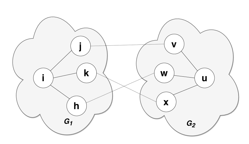
Figure 2: Example of Rule 1

Figure (2) illustrates an example graph under Rule 1 where dashed lines indicate the pairs of cross-network neighbors that contribute to the computation of $\mathbf{S}^{(k)}_{i,u}$. For example, if the similarity between $j_{(1)}$ and $v_{(2)}$ is accumulated into $\mathbf{S}^{(k)}_{i,u}$, then the similarity between ($j_{(1)}$, $w_{(2)}$), ($j_{(1)}$, $x_{(2)}$), ($k_{(1)}$, $v_{(2)}$), and ($h_{(1)}$, $v_{(2)}$) can no longer contribute to $\mathbf{S}^{(k)}_{i,u}$.

Formally, Rule 1 decreases the number of pairs of cross-network contributing neighbors from $|N(i_{(1)})||N(u_{(2)})|$ to at most $\min\{|N(i_{(1)})|,|N(u_{(2)})|\}$. This setting provides an effective way to penalize the degree differences (as shown later). Additionally, it reduces the amount of “noisy” similarities included during the iteration process.

3.1.2 Rule 2 – level-two elimination

Prior to defining Rule 2, we assume that Rule 1 is satisfied. As we have defined previously, a pair of cross-network neighbors can be aligned if at least one of them is globally most similar to the other. Because of the iterative nature of ELRUNA, however, during the first several iterations of the algorithm, the computed similarities are less revealing of the true similarities between vertices. In other words, we are less certain about whether the node that is globally most similar to $j_{(1)}$ is indeed its best match. Therefore, for each iteration, allowing only most similar pairs of neighbors globally to contribute while discarding others might fail to accumulate valuable information.

We want to relax this constraint. We observe that as we proceed with more iterations, the reliability of similarities increases. To model this increase of confidence, we define growing thresholds such that under Rule 1, pairs of neighbors whose similarities are greater than their thresholds are allowed to contribute. Such thresholds are low at the first iteration and grow gradually as we proceed with more iterations.

We define vectors $\mathbf{b1}$ and b2 for two networks respectively such that

$$\textbf{b1}^{(k)}_{i}=\max_{u\in V_{2}}\textbf{S}^{(k)}_{i,u}\text{ and }\textbf{b2}^{(k)}_{u}=\max_{i\in V_{1}}\textbf{S}^{(k)}_{i,u}.$$

Informally, $\textbf{b1}^{(k)}_{i}$ is the similarity between $i_{(1)}$ and its globally most similar vertex at the $k$th iteration. Additionally, we define contribution-threshold vectors c1 and c2 for two networks. Given a pair of vertices $(i_{(1)},u_{(2)})$, a pair of their cross-network neighbors $(j_{(1)},v_{(2)})$ can contribute similarity to $\mathbf{S}^{(k+1)}_{i,u}$ only if $\textbf{S}^{(k)}_{j,v}\geq\min\{\textbf{c1}^{(k)}_{j}\;,\textbf{c2}^{(k)}_{v}\}$. At the same time, such thresholds grow as the algorithm proceeds with more iterations.

Computing the similarity between $(i_{(1)},u_{(2)})$ iteratively can be seen as a process of gathering information (regarding the similarity) from other nodes in a breadth-first search manner such that $\textbf{S}^{(k)}_{i,u}$ is computed based on similarities between cross-network nodes that are within distance $k$ away from $i_{(1)}$ and $u_{(u)}$. A node $j_{(1)}$ is said to be visited by $i_{(1)}$ at the the $k$th iteration if $j_{(1)}$ is within distance $k$ away from $i_{(1)}$. We use the fraction of visited nodes after each iteration as a measure to model the increase of the contribution threshold. We now define the contribution threshold formally.

Definition 4 (Contribution Threshold).

Given $G_{1}$ with size $n_{1}$, let T1 be the $n_{1}\times t_{max}$ matrix for which $\text{\bf{T1}}_{i,k}$ is the fraction of nodes that $i_{(1)}$ has visited after the $k$th iteration. Then the contribution threshold of $i_{(1)}$, denoted by $\text{\bf{c1}}_{i}$, after the $k$th iteration is defined as

$$\text{\bf{c1}}^{(k)}_{i}=\text{\bf{b1}}^{(k)}_{i}\cdot\text{\bf{T1}}_{i,k}.$$ (4)

$\mathbf{T1}_{i,0}=1/n_{1}$ for all $i_{(1)}\in{V}_{1}$. As $k$ approaches $t_{max}$, $\mathbf{T1}_{i,k}$ approaches $1$ and $\textbf{c}^{(k)}_{i}$ approaches $\textbf{b}^{(k)}_{i}$. $\mathbf{c2}$ and $\mathbf{T2}$ are defined for $G_{2}$ in the same fashion. The pseudocode for computing T1 and $\mathbf{T2}$ is shown in Algorithm (1).

Input: ${G}=({V},{E})$, $t_{max}$

1

Output: Contribution threshold matrix T

2

3$\textbf{T}\leftarrow n\times t_{max}$ zero-matrix $\triangleright$ $|{V}|=n$

4

5for $i\in{V}$ do

6       $\textbf{d}\leftarrow n\times 1$ vector with all entries equal to $0$

7       $\textbf{d}_{i}=1$

8       $num\_of\_visited\_node\leftarrow$ $1$

9       $frontier\leftarrow$ empty list.

10       $frontier$.insert($i$)

11       for $k\leftarrow 1$ to $t_{max}$ do

12             $new\_frontier\leftarrow$ empty list.

13             for $j$ in $frontier$ do

14                   for $q$ in ${N}(j)$ do

15                         if $\textbf{d}_{q}$ == $0$ then

16                               $num\_of\_visited\_node+=1$

17                               $new\_frontier$.insert($q$)

18                               $\textbf{d}_{q}=1$

19                              

20                        

21                  

22            $\textbf{T}_{i,k}=\frac{num\_of\_visited\_node}{n}$

23             $frontier=new\_frontier$

24            

25      

26return T

Algorithm 1 Contribution Threshold

Let $(j_{(1)},v_{(2)})$ be a pair of cross-network neighbors of $(i_{(1)},u_{(2)})$. Without loss of generality, suppose $\textbf{S}^{(k)}_{j,v}\geq\textbf{c1}^{(k)}_{j}$ but $\textbf{S}^{(k)}_{j,v}<\textbf{c2}^{(k)}_{v}$. This implies that there must exist a better alignment with higher similarity for $v_{(2)}$ at the $k$th iteration. We still want to accumulate the similarity between $j_{(1)}$ and $v_{(2)}$ to $\textbf{S}^{(k)}_{i,u}$. At the same time, we should also consider the loss of similarity by aligning $j_{(1)}$ to $v_{(2)}$ (recall that we model similarity accumulation as a process of aligning neighbors). We introduce a simple measure called net similarity:

$$\textbf{N}^{(k)}_{jv}=2\textbf{S}^{(k)}_{j,v}-\left[\frac{\textbf{S}^{(k)}_{j,v}-\textbf{c1}^{(k)}_{j}}{\textbf{b1}^{(k)}_{j}-\textbf{c1}^{(k)}_{j}}\cdot(\textbf{b2}^{(k)}_{v}-\textbf{c2}^{(k)}_{v})+\textbf{c2}^{(k)}_{v}\right]$$ (5)

and if $\textbf{S}^{(k)}_{j,v}\geq\textbf{c2}^{(k)}_{v}$ but $\textbf{S}^{(k)}_{j,v}<\textbf{c1}^{(k)}_{j}$,

$$\textbf{N}^{(k)}_{jv}=2\textbf{S}^{(k)}_{j,v}-\left[\frac{\textbf{S}^{(k)}_{j,v}-\textbf{c2}^{(k)}_{v}}{\textbf{b2}^{(k)}_{v}-\textbf{c2}^{(k)}_{v}}\cdot(\textbf{b1}^{(k)}_{j}-\textbf{c1}^{(k)}_{j})+\textbf{c1}^{(k)}_{j}\right],$$ (6)

which leads to our second rule.

1. Rule 2. Given a pair of cross-network vertices $(j_{(1)},v_{(2)})$, under Rule 1, the amount of similarity they can contribute to a pair of neighbors $(i_{(1)},u_{(2)})$ is

   $$\begin{cases}\mathbf{S}^{(k)}_{j,v}&\text{if $\textbf{S}^{(k)}_{j,v}\geq\max\{\textbf{c1}^{(k)}_{j},\;\textbf{c2}^{(k)}_{v}$\} }\\ \mathbf{N}^{(k)}_{j,v}&\text{if $\min\{\textbf{c1}^{(k)}_{j},\;\textbf{c2}^{(k)}_{v}\}\leq\mathbf{S}^{(k)}_{j,v}\leq\max\{\textbf{c1}^{(k)}_{j},\;\textbf{c2}^{(k)}_{v}\}$ }\\ 0&\text{otherwise}.\\ \end{cases}$$

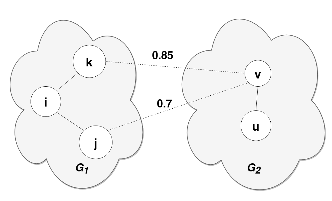
Figure 3: Example of Rule 3

3.1.3 Rule 3 – Prioritization

Given the first two rules, it is possible that a neighbor of $u_{(2)}$ is globally most similar to multiple neighbors of $i_{(1)}$ but with different similarities. For example, consider a sample graph shown in Figure (3) where $v_{(2)}$ is globally most similar to both $j_{(1)}$ and $k_{(1)}$. Dashed lines indicate the similarities between two vertices.

In this case, we ought to consider only the pair $(k_{(1)},v_{(2)})$ and contribute its similarity to $\mathbf{S}_{i,u}$, which leads to the final rule.

1. Rule 3. During the computation of the similarity between $i_{(1)}$ and $u_{(2)}$, a pair of cross-network neighbors with a higher similarity should be given prior consideration.

3.1.4 The Similarity Computation Algorithm

The general idea of the ELRUNA is to update $\mathbf{S}$, $\mathbf{b1}$ and $\mathbf{b2}$ iteratively based on their values in the previous iteration. The initial similarities between each pair of cross-network vertices are uniformly distributed. We set them all equal to $1$. That is, $\mathbf{S}^{(0)}$ is a matrix of ones. Note that many other algorithms require prior knowledge about the similarities (usually based on non-network information) between vertices, whereas ELRUNA does not require such knowledge.

The detailed algorithm is summarized in Algorithm (2). Overall, at the $(k-1)$th iteration, for each pair of cross-network vertices ($i_{(1)},u_{(2)}$), we first check all pairs of their cross-network neighbors against Rule 2 to determine which pairs are qualified such that the similarity is greater than the contribution threshold of at least one node in the pair. Then we sort those pairs by similarities in descending order, which is needed to follow Rule 3. After sorting, we go over each ($j_{(1)},v_{(2)}$) in the sorted order, checking $j_{(1)}$ and $v_{(2)}$ against Rule 1. If none of them has contributed to $\mathbf{S}^{(k)}_{i,u}$ before, we accumulate the similarity between $(j_{(1)},v_{(2)})$ based on Rule 2 and mark $j_{(1)}$ and $v_{(2)}$ as selected, which indicates that they can no longer be considered. This step enforces Rule 1. Note that the selected neighbors will no longer be selected after we are done computing $\mathbf{S}^{(k)}_{i,u}$. We now update $\textbf{S}^{(k)}$, $\textbf{b1}^{(k)}$, and $\mathbf{b2}^{(k)}$.

After accumulating similarities from neighbors, we normalize it by

$$\textbf{S}^{(k+1)}_{iu}=\frac{\text{accumulated similarity}}{\max\{\sum_{j\in{N}(i)}\textbf{b1}^{(k)}_{j},\sum_{v\in{N}(u)}\textbf{b2}^{(k)}_{v}\}}.$$

$\textbf{S}^{(k+1)}_{iu}$ is set to $0$ if $\max\{\sum_{j\in{N}(i)}\textbf{b1}^{(k)}_{j},\sum_{v\in{N}(u)}\textbf{b2}^{(k)}_{v}\}=0$. This normalization also penalizes the degree of discrepancy between $i_{(1)}$ and $u_{(2)}$ because the maximum number of pairs of cross-network neighbors that can contribute similarity to ($i_{(1)},u_{(2)}$) is upper bounded by the smaller degree between $i_{(1)}$ and $u_{(2)}$.

The similarity computation step of ELRUNA consists of running Algorithm (1) and (2), which outputs the final similarity matrix $\mathbf{S}$.

Input: ${G}_{1}=({V}_{1},{E}_{1})$ , ${G}_{2}=({V}_{2},{E}_{2})$, $t_{max},\textbf{T1},\textbf{T2}$

1

Output: The similarity matrix S

2

3for $k\leftarrow 1$ to $t_{max}$ do

4       $\text{\bf{S}}^{(k)}\leftarrow n_{1}\times n_{2}$ similarity matrix

5       $\text{\bf{b1}}^{(k)}\leftarrow n_{1}\times 1$ vector with all entries equal to $-1$

6      

7      $\text{\bf{b2}}^{(k)}\leftarrow n_{2}\times 1$ vector with all entries equal to $-1$

8      

9      Update $\mathbf{c1}^{(k-1)}$ and $\mathbf{c2}^{(k-1)}$ based on Equation 4

10      

11      for $i$ in ${V}_{1}$ do

12             for $u$ in ${V}_{2}$ do

13                   $\mathbf{e}\leftarrow$ empty associative array

14                   $sum\leftarrow$ $0$

15                   for $j$ in ${N}(i)$ do

16                         for v in ${N}(u)$ do

17                               if $\mathbf{S}^{(k-1)}_{jv}\geq\min\{\mathbf{c1}^{(k-1)}_{j},\;\mathbf{c2}^{(k-1)}_{v}\}$ then

18                                     $\mathbf{e}$[($j$, $v$)] $\leftarrow$ $\mathbf{S}^{(k-1)}_{jv}$

19                                    

20                              

21                        

22                  $\mathbf{e}\leftarrow$ sort by value in descending order

23                  

24                  for $(j,v)$ in $\mathbf{e}$.keys do

25                         if $j$ and $v$ are not selected then

26                               Accumulate $sum$ based on Rule 2

27                               Mark $j$ and $v$ as selected

28                              

29                        

30                  $\mathbf{S}^{(k)}_{iu}\leftarrow\frac{sum}{\max\{\sum_{j\in{N}(i)}\mathbf{b1}^{(k-1)}_{j},\sum_{v\in{N}(u)}\mathbf{b2}^{(k-1)}_{v}\}}$

31                  

32                  if $\mathbf{S}^{(k)}_{iu}>\mathbf{b1}^{(k)}_{i}$ then

33                         $\mathbf{b1}^{(k)}_{i}=\mathbf{S}^{(k)}_{iu}$

34                  if $\mathbf{S}^{(k)}_{iu}>\mathbf{b2}^{(k)}_{u}$ then

35                         $\mathbf{b2}^{(k)}_{u}=\mathbf{S}^{(k)}_{iu}$

36                  

37            

38      

return S

Algorithm 2 Similarity Computation

We have added pictorial examples of Rule 1 and Rule 3 in the Appendix for a better demonstration of the algorithm.

3.2 Step 2: Building Alignment of Vertices

After obtaining the final cross-network similarity matrix $\mathbf{S}$, we use two methods to extract the mappings between vertices from two networks: naive and seed-and-extend alignment.

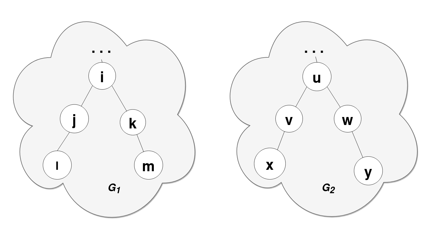
Figure 4: Failure of naive alignment to distinguish symmetric nodes

3.2.1 Naive Alignment

Following the literature [38], we sort all pairs of cross-network vertices by similarities in descending order. Then we iteratively align the next pair of unaligned vertices until all nodes in the smaller network are aligned. We note that this is a relatively simple alignment method, while many other algorithms [13, 20, 6, 8, 9, 2, 22] use more complicated and computationally expensive alignment methods. As shown in the experimental section, however, using this naive alignment method, ELRUNA significantly outperforms other baselines.

While the naive alignment method produces alignments of competitive quality, we observe that it fails to distinguish nodes that are topologically symmetric. An example is shown in Figure (4) where ${G}_{1}$ and ${G}_{2}$ are isomorphic. In this circumstance, $k_{(1)}$ is equally similar to $v_{(2)}$ and $w_{(2)}$. At the same time, $m_{(1)}$ is equally similar to $x_{(2)}$ and $y_{(2)}$. If we break ties randomly, it is possible that $k_{(1)}$ and $m_{(1)}$ may be mapped to vertices on different branches of the tree, causing the loss of the number of conserved edges.

3.2.2 Seed-and-Extend Alignment

During the alignment process, nodes that have been aligned can serve as guidance for aligning other nodes [20]. Referring back to Figure (4), aligning $k_{(1)}$ to $w_{(2)}$ should imply that $m_{(1)}$ ought to be aligned with $y_{(2)}$ rather than $x_{(2)}$. To address the limitation of the naive alignment methods, we iteratively find the pair of unaligned nodes with the highest similarity. Then we align them and increase similarities between every pair of their unaligned cross-network neighbors by some small constant. Iterations proceed until all nodes in the smaller network are aligned. For efficiency, we use a red-black tree to store pairs of nodes.

3.3 Time Complexity of ELRUNA

Without loss of generality, we assume that two networks have a comparable number of vertices and edges. Let $n$ and $m$ denote the number of vertices and edges, respectively. Let $t_{max}$ denote the total number of iterations. One can easily see that Algorithm (1) runs in $O(n^{2}+mn)$ time and the naive alignment method runs in $O(n^{2}\log n)$ time.

Lemma 1.

The time complexity of Algorithm (2) is $O(t_{max}m^{2}\log n)$.

Proof.

Let $d_{i}$ denote the degree of vertex $i_{(1)}$. Operations on lines $12$ to $13$ and lines $19$ to $23$ take constant time; thus the nested for loops on lines $10$ to $13$ take $\Theta(d_{i}d_{u})$ time for every pair of $i_{(1)}$ and $u_{(2)}$. Sorting on line $14$ takes $\Theta(d_{i}d_{u}\log d_{i}d_{u})$ time, and the for loop on lines $15$ to $18$ takes $\Theta(d_{i}d_{u})$ time. We observe that $O(\log d_{i}d_{u})=O(\log n^{2})=O(\log n)$; therefore, the outer nested for loop on lines $6$ to $23$ takes

$$O(\sum_{i\in{V}_{1}}\sum_{u\in{V}_{2}}d_{i}d_{u}\log(d_{i}d_{u})) =O(\log n\sum_{i\in{V}_{1}}d_{i}\sum_{u\in{V}_{2}}d_{u})$$ (7)

$$=O(m^{2}\log n).$$

The time complexity of the Algorithm (2) is $O(t_{max}\cdot m^{2}\log n)$. ∎

Lemma 2.

The time complexity of the seed-and-extend alignment method is $O((n^{2}+mn)\log(n^{2}+mn))$.

Proof.

At the beginning of the algorithm, adding all $n^{2}$ pairs of nodes into the red-black tree takes $O(n^{2}\log n)$ time. Whenever we align a pair of vertices ($i_{(1)},u_{(2)}$), we increase the similarities between all pairs of their unaligned cross-network neighbors. To update the corresponding similarities in the red-black tree, we add those pairs with new similarities into the tree. The total number of insertions of such pairs is

$$\sum_{i_{(1)}\in{V}_{1}}d_{i}d_{f(i)},$$

where $f(i)\in{V}_{2}$ is the node that $i_{(1)}$ is aligned to. One can easily see that the function above is upper bounded by $O(mn)$, which implies that the total number of elements in the tree is $O(n^{2}+mn)$. We perform at most $n^{2}+mn$ number of find_max, deletion, and insertion operations; therefore, the overall running time of the algorithm is $O((n^{2}+mn)\log(n^{2}+mn))$. ∎

The overall running time of the proposed ELRUNA is $O(t_{max}\cdot m^{2}\log n)$. If we assume that $O(m)=O(n\log n)$, which is a fair assumption for the networks that are used in the experiments, then the overall running time is $O(t_{max}\cdot n^{2}\log^{3}n)$.

4 RAWSEM : Random-Walk-Based Selection Method

In this section, we introduce the proposed selection rule RAWSEM for our local search procedure. We first discuss the baseline, which is used as the comparison method with RAWSEM. We then present the mechanism of RAWSEM.

4.1 The Baseline

The aim of the baseline is to further improve the objective value. Following the literature [28], given the permutation matrix produced by any alignment algorithm, the baseline algorithm constructs the search space for local search by selecting a subset of vertices from the smaller network and generating all permutations of their alignments while fixing the alignment of all other vertices that are not in the subset [28] For each of the permutation of the alignment between selected vertices, the baseline selects the one that improves the objective the most. The baseline iterates until the objective has not been improved for a fixed number of iterations.

Given ${G}_{1}=({V}_{1},{E}_{1})$ and ${G}_{2}=({V}_{2},{E}_{2})$, we transform the alignment matrix P to the $n_{1}\times 1$ alignment vector $\widetilde{\Pi}$ for which $\widetilde{\Pi}_{i}=u_{(2)}$ implies that vertex $i_{(1)}$ is aligned to vertex $u_{(2)}$.

For each iteration, we randomly select a subset of vertices ${V}_{1}^{\prime}\subset{V}_{1}$ with a fixed cardinality. Let ${V}_{2}^{\prime}=\{\widetilde{\Pi}_{i}:i\in{V}_{1}^{\prime}\}$. Let $\mathbf{A}$ and $\mathbf{B}$ be the adjacency matrices of $G_{1}$ and $G_{2}$, respectively. The baseline local search explores all feasible solutions in the search space and attempts to find a new alignment vector $\Pi$ with a lower objective:

$$\min_{\Pi} \{-\frac{1}{2}\sum_{i,j\in{V}_{1}^{\prime}}(\textbf{A}_{ij}\textbf{B}_{\Pi_{i}\Pi_{j}}+\sum_{k\in{N}(i)|k\notin{V}_{1}^{\prime}}\textbf{A}_{ik}\textbf{B}_{\Pi_{i}\widetilde{\Pi}_{k}}+$$ (8)

$$\sum_{p\in{N}(j)|p\notin{V}_{1}^{\prime}}\textbf{A}_{jp}\textbf{B}_{\Pi_{j}\widetilde{\Pi}_{p}})\}$$

$$\text{s.t.}\;\;\Pi_{i}\in{V}_{2}^{\prime}\;\;\forall i\in{V}_{1}^{\prime}.$$

The baseline local search proceeds until the optimum has been reached, meaning that the objective has not been improved in over a number of iterations.

4.2 RAWSEM Algorithm

Depending on the quality of the initial solution, it is possible that only a small fraction of vertices are not mapped optimally. Therefore, the baseline approach, which constructs the subset ${V}^{\prime}_{1}$ with random selections from the entire vertex set, is not efficient. Ideally, we want to locate vertices that are not mapped optimally and only permute the alignments between them.

For simplicity, suppose nodes in ${V}_{1}$ are labeled with consecutive integers starting from $1$ and that nodes in ${V}_{2}$ are labeled with consecutive integers starting from $|{V}_{1}|+1$. To quantify the level of mismatching of each vertex, we first define the concept of violation.

Definition 5 (Violation).

Let $\mathbf{o^{\prime}}$ be an $n_{1}\times n_{2}$ by $1$ vector. The violation value of a vertex $i_{(1)}\in{G}_{1}$ is defined as

$$\mathbf{o}^{\prime}_{i} =\sum_{j\in{N}(i)}(1-\mathbf{B}_{\widetilde{\Pi}_{i},\widetilde{\Pi}_{j}})$$ (9)

$$=|{N}(i)|-\sum_{j\in{N}(i)}\mathbf{B}_{\widetilde{\Pi}_{i},\widetilde{\Pi}_{j}}.$$

Informally, $\mathbf{o}^{\prime}_{i}$ is the number of the neighbors of $i_{(1)}$ that are not conserved by $i_{(1)}$.

Let $\bar{{V}}_{2}=\{u_{(2)}\in{V}_{2}\;:\;\widetilde{\Pi}_{i}=u_{(2)}\;\exists\;i_{(1)}\in{V}_{1}\}$ be the subset of ${V}_{2}$ consisting of all aligned vertices in $G_{2}$. Let $\widetilde{\Pi}^{-1}:\bar{{V}}_{2}\rightarrow{V}_{1}$ be the inverse mapping. Then the violation value of vertex $u\in{V}_{2}$ is defined in the same fashion:

$$\mathbf{o}^{\prime}_{u} =\sum_{v\in{N}(u)}(1-\mathbf{A}_{\widetilde{\Pi}^{-1}_{u},\widetilde{\Pi}^{-1}_{v}})$$ (10)

$$=|{N}(u)|-\sum_{v\in{N}(u)}\mathbf{A}_{\widetilde{\Pi}^{-1}_{u},\widetilde{\Pi}^{-1}_{v}}.$$

We normalize violations of vertices by their degrees. Let $\mathbf{o}$ be a vector that encodes the normalized violation value of each vertex. Then we have

$$\mathbf{o}=\mathbf{D}^{-1}\mathbf{o^{\prime}},$$ (11)

where $\mathbf{D}$ is the diagonal degree matrix such that $\mathbf{D}_{i,i}$ is the degree of vertex $i$. $\mathbf{o}$ provides the initial level of mismatching of each vertex. We further normalize $\mathbf{o}$ such that its $L1$ norm equals $1$.

From a high level, RAWSEM is a two-step procedure.

1. (1) Ranking vertices: Starting from the initial level of mismatching of vertices, RAWSEM iteratively updates $\mathbf{o}$ in a PageRank [21] fashion. Then, it ranks vertices by the converged levels of mismatching.

2. (2) Local search: The search space is constructed based on the ranking, and the local search is performed.

4.2.1 Step 1 – Ranking Vertices

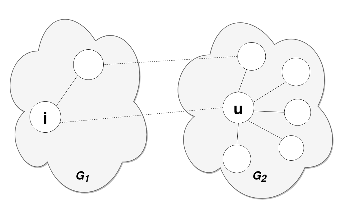
Figure 5: Zero violation of vertex $i$

For two real-world networks where isomorphism does not exist, we expect many vertices to have nonzero initial violations. Clearly, a nonzero violation does not imply a non-optimal mapping. We note that a zero violation does not always imply an optimal mapping. As shown in the Figure (5) where dashed lines indicate mappings, $i_{(1)}$ has a zero violation. This suggests the insufficiency of initial violation values.

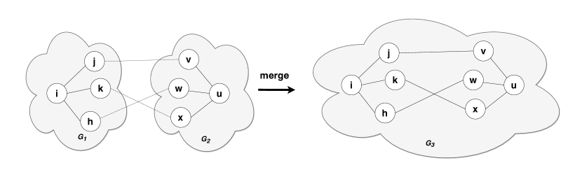
Figure 6: Example of the merge operation

To adapt the network information into our model, we use an iterative approach based on the intuition that a vertex is more mismatched if its neighbors are more mismatched. One immediate method is to propagate a violation value via edges throughout the networks. Let ${G}_{2}^{\prime}=(\bar{{V}}_{2},\bar{{E}}_{2})$ be the subgraph induced by $\bar{{V}}_{2}$ (as stated above, $\bar{{V}}_{2}$ is the set of aligned vertices in $G_{2}$). To start with, we merge ${G}_{1}$ and ${G}_{2}^{\prime}$ by adding edges to connect aligned cross-network vertices. Figure (6) illustrates a example of the merge operation. We denote the newly constructed undirected graph ${G}_{3}=({V}_{3},{E}_{3})$, where ${V}_{3}={V}_{1}\cup\bar{{V}}_{2}$ and ${E}_{3}={E}_{1}\cup\bar{{E}}_{2}\cup\{(i_{(1)},u_{(2)}):i_{(1)}\in{V}_{1},u_{(2)}=\widetilde{\Pi}_{i}\}$. Let C denote the adjacency matrix of ${G}_{3}$. Let R be the vector that encodes the propagated levels of mismatching for each vertex. Let D denote the diagonal degree matrix such that $\textbf{D}_{i,i}=|{N}(i)|$. We propagate violations in a PageRank [21] fashion:

$$\textbf{R}^{(k)}_{i}=\alpha\sum_{j}\frac{\textbf{C}_{ij}}{\textbf{D}_{j,j}}\textbf{R}^{(k-1)}_{j}+(1-\alpha)\textbf{o}_{i}.$$ (12)

In matrix notation, this is

$$\textbf{R}^{(k)}=\alpha\textbf{CD}^{-1}\textbf{R}^{(k-1)}+(1-\alpha)\textbf{o}.$$ (13)

By initializing $\mathbf{R}^{(0)}$ as a probability vector, we can rewrite Equation (13) to

$$\textbf{R}^{(k)}=[\alpha\textbf{CD}^{-1}+(1-\alpha)\textbf{o}\textbf{1}^{T}]\;\textbf{R}^{(k-1)},$$ (14)

where $\mathbf{1}$ is the vector with all entries equal to $1$.

Equation (14) encodes an eigenvalue problem that can be approximated by power iteration. Let $\textbf{E}=\alpha\textbf{CD}^{-1}+(1-\alpha)\textbf{o}\textbf{1}^{T}$. By the undirected nature of ${G}_{3}$, the transition matrix $\textbf{C}\textbf{D}^{-1}$ is irreducible; therefore E is a left-stochastic matrix with a leading eigenvalue equal to $1$, and the solution of Equation (14) is the principal eigenvector of E. Moreover, E is also primitive; therefore the leading eigenvalue of E is unique, and the corresponding principal eigenvector can be chosen to be strictly positive. As a result, the power iteration converges to its principal eigenvector.

The violation vector o plays the role of teleportation distribution, which encodes external influences on the importance of vertices. The converged R gives the levels of mismatching of vertices, and a vertex with a higher value is even more mismatched. We rank vertices in $G_{1}$ based on $\mathbf{R}$ in descending order.

4.2.2 Step 2 – Local Search

Based on the ranking produced in the previous step, RAWSEM uses a sliding window over sorted vertices to narrow down the search space. Let $m$ be the size of the window with the tail lying at the highest-ranked vertices. For each iteration, we construct ${V}^{\prime}_{1}$ by randomly selecting vertices within the window and perform the local search. If the objective has not been improved in $s$ iterations, we move the window $l$ nodes forward, then continue the local search procedure. The local search terminates when the objective has not been improved for $s_{max}$ number of iterations. In our experiments, we set $|{V}_{1}|=6$.

5 Experimental Results

In this section, we first present the experimental setup and performance of the proposed ELRUNA in comparison with $8$ baseline methods over three alignment scenarios. Then, we study the time-quality trade-off and the scalability of ELRUNA. We emphasize that ELRUNA is not a local search method and should not be compared with local search methods because ELRUNA can serve as a preprocessing step to all local searches. We demonstrate that RAWSEM could further improve the alignment quality with significantly fewer iterations than the naive local search method requires.

Reproducibility: Our source code, documentation, and data sets are available at https://tinyurl.com/uwn35an.

Baselines for ELRUNA. We compare ELRUNA with 8 state-of-the-art network alignment algorithms: IsoRank [31], Klau [13], NetAlign [2], REGAL [11], EigenAlign [6], C-GRAAL [19], NETAL [20], and HubAlign [9]. These algorithms, published in years 2008–2019, have proven superior to many other methods, so we choose them. Other methods that perform in significantly longer running time have not been considered. The baseline methods are described in the Related Work section. C-GRAAL, Klau and Netalign require prior similarities between cross-network vertices as input. Following [38, 11], we use the degree of similarities as the prior similarities. For Klau and Netalign, as suggested by [11], we construct the prior alignment matrix by choosing the highest $k\times\log_{2}n$ vertices, where $k=5$. Note that ELRUNA does not requires prior knowledge about the similarities between cross-network vertices.

We do not compare ELRUNA with FINAL [38] because FINAL solves a different problem, namely, the attributed network alignment problem. ModuleAlign [8] is also not chosen as a baseline method because it is the same as HubAlign [9] except that ModuleAlign uses a different method to optimize the biological similarities between vertices. Additionally, we do not compare with GHOST [22] because its signature extraction step took hours even for small networks.

Experimental Setup for ELRUNA. All experiments were performed on an Intel Xeon E5-2670 machine with 64 GB of RAM. For the sake of iterative progress comparison, we set the maximum number of iterations $t_{max}$ to the larger diameter of the two networks.

Our experiment consists of three scenarios: (1) self-alignment without and under the noise, (2) alignment between homogeneous networks, and (3) alignment between heterogeneous networks. Detailed descriptions of each category are presented later. In general, the first test scenario self-alignment without and under the noise consists of 12 networks from various domains. For each network, we generate up to 14 noisy copies with increasing noise levels (defined later) up to $25\%$. This gives us a total of $1,64$ pairs of a network to align. The second test scenario alignment between homogeneous networks has $3$ pairs of networks for which each pair consists of two subnetworks of a larger network. In our third test scenario alignment between heterogeneous networks, we align 5 pairs of networks where each pair consists of two networks from different domains. We note that the third scenario is usually used by attributed network alignment algorithms. Therefore, it is not exactly what we solve with our formulation, but we demonstrate the results because it is an important practical task. To the best of our knowledge, our experimental setup is the most comprehensive in terms of the combination of the number of baselines, the number of networks, the categories of testing cases, and the levels of noise applied.

Evaluation Metric. To quantify the alignment quality, we use two well-known metrics: the edge correctness (EC) [20] and the symmetric substructure score ($S^{3}$) [27]. Let $f(V_{1})=\{u\in V_{2}:\mathbf{P}_{i,u}=1,\exists i\in V_{1}\}$, and $f(E_{1})=|\{(f(i_{(1)}),f(j_{(1)}))\in E_{2}\;:\;(i_{(1)},j_{(1)})\in E_{1}\}|$. That is, $f(V_{1})$ is the set of vertices in $G_{2}$ that are aligned (note that since we assume $|V_{1}|\leq|V_{2}|$, some vertices in $G_{2}$ are left unaligned), and $f(E_{1})$ is the set of edges in $G_{2}$ such that for each edge, the alignment of its incident vertices is adjacent in $G_{1}$. Then, we have

$$EC=\frac{|f(E_{1})|}{|E_{1}|}$$ (15)

and

$$S^{3}=\frac{|f(E_{1})|}{|E_{1}|+|E(G_{2}[f(V_{1})])|-|f(E_{1})|},$$ (16)

where $|E(G_{2}[f(V_{1})])|$ is the number of edges in the subgraph of $G_{2}$ induced by $f(V_{1})$.

5.1 Self-alignment without and under the Noise

In this experiment, we analyze how ELRUNA performs with structure noise being added to the original network. Given a target network $G_{1}$, simply aligning $G_{1}$ with its random permutations is not a challenge for most of the existing state-of-the-art network alignment algorithms. A more interesting test case arises when we try to align the original networks $G_{1}$ with its noisy permutations $G_{2}$ such that $G_{2}$ is a copy of $G_{1}$ with additional edges being added [20, 14, 38, 37, 10]. This scenario is even more challenging when the number of noisy edges is large with respect to the number of edges in $G_{1}$. In addition, this perturbation approach reflects many real-life network alignment task scenarios [2, 10, 11].

Given the network ${G}_{1}=({V}_{1},{E}_{1})$, a noisy permutation of ${G}_{1}$ with noise level $p$, denoted by ${G}^{(p)}_{2}=({V}_{2},{E}_{2})$, is created with two steps:

1. Permute ${G}_{1}$ with some randomly generate permutation matrix.

2. Add $p|{E}_{1}|$ edges to ${G}_{1}$ uniformly at random by randomly connecting nonadjacent pairs of vertices.

Properties of each network $G_{1}$ are given in Table 5.1. Note that under this model, the highest EC any algorithm can achieve by aligning ${G}_{1}$ and ${G}_{2}$ is always $1$. In this experiment, we demonstrate the results without applying local search; that is, we demonstrate how only ELRUNA outperforms the state-of-the-art methods.

tableNetworks for test case: self-align without and under noise Domain $n$ $m$ label Barabasi random network 400 2,751 barabasi Homle random network 400 2,732 homel Coauthorships 379 914 co-auth_1 Gene functional association 993 1,300 bio_1 Economy 1,258 7,513 econ Router 2,113 6,632 router Protein-protein interaction 2,831 4,562 bio_2 Twitter 4,171 7,059 retweet_1 Erods collaboration 5,019 7,536 erdos Twitter 7,252 8,061 retweet_2 Social interaction 10,680 24,316 social Google+ 23,628 39,242 google+

To demonstrate the effectiveness of ELRUNA, we first solve the alignment problems on random networks generated by Baràbasi–Albert preferential attachment model (BA model) [1] and the Holme-Kim model (HK model) [12]; see Table 5.1. The HK model reinforces the BA model with an additional probability $q$ of creating a triangle after connecting a new node to an existing node. In our experiment we set $q=0.4$. For each of the random networks, we generate $12$ noisy permutations with increasing noise level $p$ from 0 to 0.21. We then align ${G}_{1}$ with each of its noisy permutations using ELRUNA and the baseline algorithms. ELRUNA has two versions, ELRUNA_Naive and ELRUNA_Seed, which differ by the alignment methods we use. The results are summarized in Figures 7 and 8.

Next, we solve the network alignment problem on 10 real-world networks [24, 16, 3] from various domains. The details of the selected networks are shown in Table 5.1. For each network, we use the same model to generate $14$ noisy permutations with increasing noise level $p$ from $0$ up to $0.25$. That is, $G_{2}^{(0.25)}$ has added additional $25\%$ noisy edges added to $G_{1}$. We then align $G_{1}$ with each of its permutation using ELRUNA and the baseline algorithms. The results are summarized in Figures 9–18.

Similar to most existing state-of-the-art network alignment algorithms’ testsets, the networks in our testset are sparse. This is one of the common limitations of the similarity matrix based approaches. Aligning dense graphs implies using dense similarity matrices (or comparable data structures that replace these matrices). Implementing scalable alignment algorithms for dense graphs that actually effectively manipulate dense similarity matrices requires a lot of effort (such as extremely fast matrix manipulations, parallelization, and specific dense data structures that are potentially different for different hardware) that is beyond the scope of this work because the focus will actually be more on the performance rather than the trade-off of quality and performance. To the best of our knowledge, the most competitive network alignment approaches are lack of effective implementation for dense graphs.

Results. Clearly, ELRUNA significantly outperforms all baselines on all networks. In particular, both versions of ELRUNA (ELRUNA_Naive and ELRUNA_Seed) outperform 6 existing methods—REGAL, EigenAlign, Klau, IsoRank, C-GRAAL, and NetAlign—by an order of magnitude under high noise levels. For the other two baselines, NETAL and HubAlgin, ELRUNA also produces much better results than they do, with improvement up to $60\%$ under high noise levels. At the same time, both versions of ELRUNA are robust to noise such that they output high-quality alignment even when $p$ reaches $0.25$. Noisy edges change the degrees of vertices by making them more uniformly distributed; in other words, they perform a process that can be viewed as network anonymization. This experiment demonstrates ELRUNA’s superiority in identifying the hidden isomorphism between two networks.

We observe that the alignment quality of Klau and NetAlign is similar. Such behaviors were also reported in other literature [11, 37]. We also note that the trends of $EC$ and $S^{3}$ are almost the same. EigenAlign crashed on bio_1 (for $p>0.17$), bio_2, econ (for $p>0.05$), router, and erdos networks, and it took over $23$ hours to even run on one instance of social, google+, and retweet_2 networks. C-GRAAL crashed on econ (ran successfully only on $p=0.3$), google+, and social networks. HubAlign crashed on google+ networks.

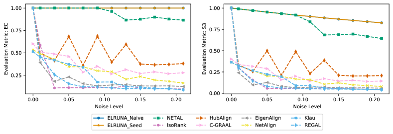
Figure 7: Alignment quality comparison on barabasi network

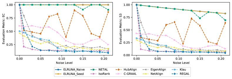
Figure 8: Alignment quality comparison on homle network

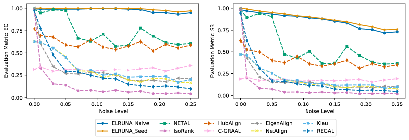
Figure 9: Alignment quality comparison on co-auth_1 network

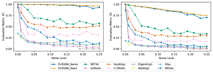
Figure 10: Alignment quality comparison on bio_1 network

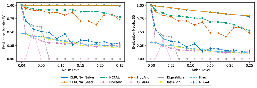
Figure 11: Alignment quality comparison on econ network

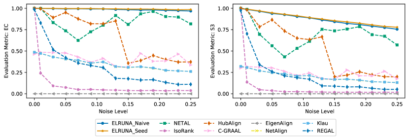
Figure 12: Alignment quality comparison on router network

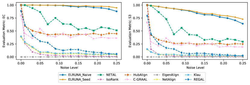
Figure 13: Alignment quality comparison on bio_2 network

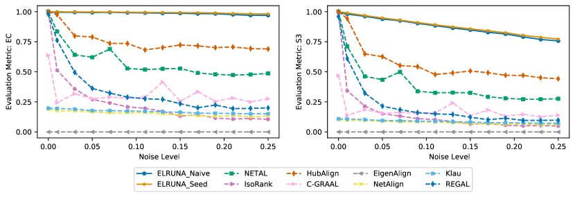
Figure 14: Alignment quality comparison on retweet_1 network

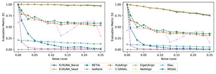
Figure 15: Alignment quality comparison on erdos network

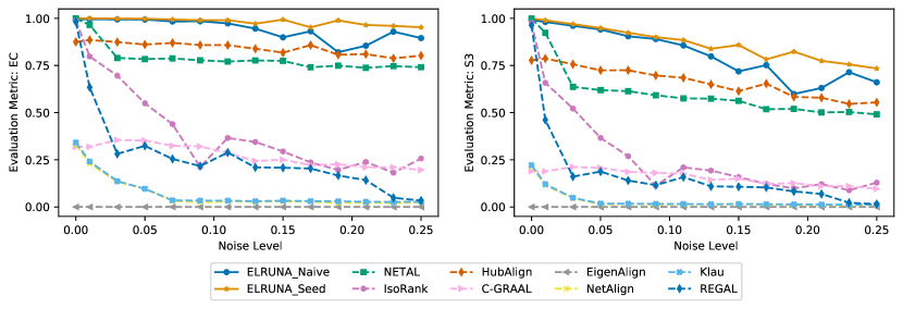
Figure 16: Alignment quality comparison on retweet_2 network

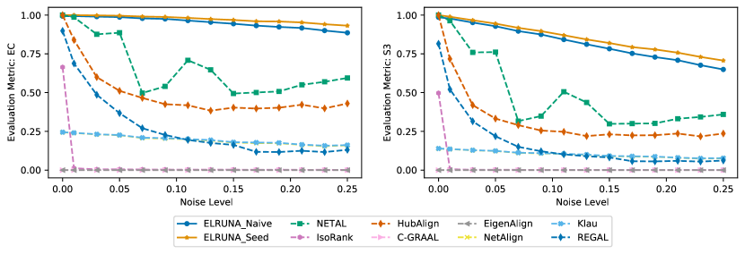
Figure 17: Alignment quality comparison on social network

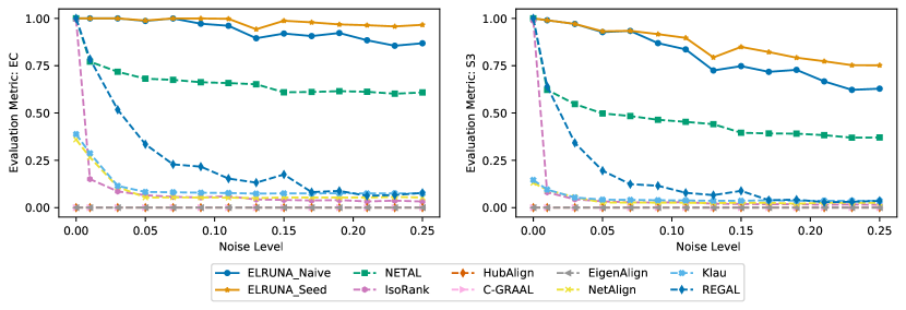
Figure 18: Alignment quality comparison on google+ network

5.2 Alignment between Homogeneous Networks

In this experiment, we study how ELRUNA performs when aligning two networks that were subgraphs of a larger network. Given a network $G$, we extract two induced subnetworks $G_{1}$ and $G_{2}$ of $G$ for which $G_{1}$ and $G_{2}$ share a common set of vertices. We compare ELRUNA_Naive and ELRUNA_Seed with the state-of-the-art methods by aligning 3 pairs of $G_{1}$ and $G_{2}$ [24, 4, 35] from 3 domains, respectively. The properties of networks are listed in Table 5.2. Note that the implementation of REGAL does not support alignment between networks with different sizes; therefore, it is not included in this testing case. In addition, the benchmark of EigenAlign is not included for the facebook networks because its running time was over 23 hours.

The first pair consists of two DBLP subnetworks with 2,455 overlapping nodes. The second pair of Digg social networks has 5,104 overlapping nodes, and the Facebook Friendship network has 8,130 nodes in common. Note that under this setting, the highest $EC$ any algorithm can achieve is lower than 1. In fact, the optimal $EC$ value is not known.

tableDatasets for test case: Alignment between homogeneous networks Domain $n$ $m$ label DBLP 3,134 vs 3,875 7,829 vs 10,594 dblp Digg Social Network 6,634 vs 7,058 12,177 vs 14,896 digg Facebook Friendship 9,932 vs 10,380 26,156 vs 31,280 facebook

In this experiment, we demonstrate the results without local search. That is, we demonstrate how ELRUNA outperforms the state-of-the-art methods. The results are shown in Figures 19, 20, and 21.

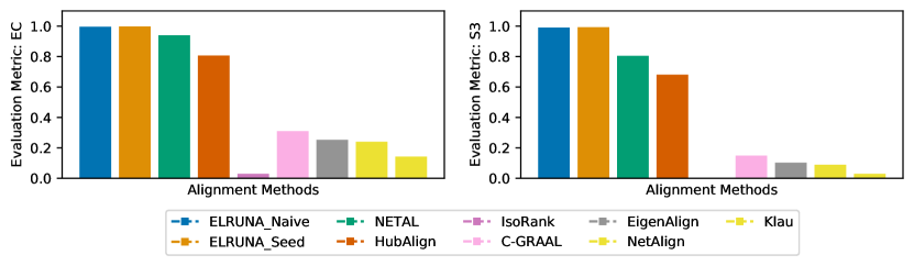
Figure 19: Alignment quality comparison on dblp networks

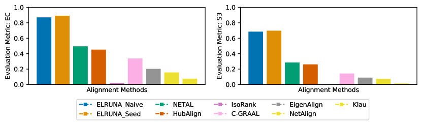
Figure 20: Alignment quality comparison on digg networks

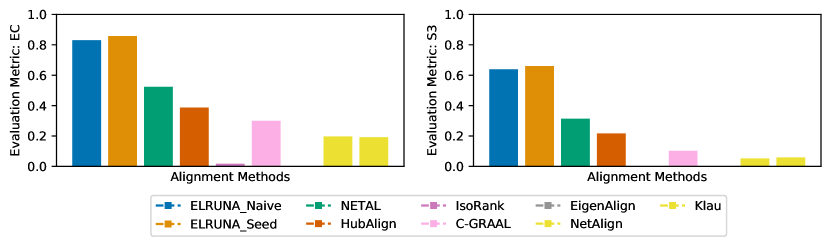
Figure 21: Alignment quality comparison on facebook networks

Results. ELRUNA outperforms all other baselines on DBLP, digg, and facebook networks. For the dblp networks, even though the $EC$ value of NETAL is close to ELRUNA (differs by $5.7734\%$), the difference between their $S^{3}$ score is more significant, with ELRUNA surpassing NETAL by $18.7728\%$. For the digg and facebook networks, ELRUNA_Naive achieves a 175.88% and a 158.45 % increase in the $EC$ score over NETAL, respectively. As of $S^{3}$, ELRUNA_Naive achieves and a 239.65% and a 203.8% increase over NETAL. At the same time, the $EC$ produced by ELRUNA_Naive is 2 to 11 times higher than for other baselines. ELRUNA_Seed outperforms ELRUNA_Naive (and therefore all baselines) with improvement of $EC$ up to 2.76% and improvement of $S^{3}$ up to 2.1% over ELRUNA_Naive.

This experiment further demonstrates the superiority of ELRUNA in identifying the underlying similar topology of networks and discovering correspondences of nodes.

5.3 Quality-Speed Trade-off and Scalability

As shown in the preceding section, ELRUNA significantly outperforms other methods in terms of alignment quality. In this section, we study the quality-speed trade-off of ELRUNA against baselines. Then, we evaluate the scalability of ELRUNA.

5.3.1 Quality-Speed Trade-off

We first evaluate the trade off by running each algorithm on the bio_1, bio_2, erdos, retweet, and social networks under the highest noise levels ($p=0.25$). That is, we align each $G_{1}$ with its corresponding $G_{2}^{(0.25)}$, then record the running time and alignment quality of each algorithm. In addition, we perform the same experiment on two pairs of networks from the homogeneous testing case: digg and facebook networks.

We measure the running time (in seconds) and alignment quality ($EC$ and $S^{3}$) of ELRUNA_Naive and ELRUNA_Seed with an incremental number of iterations. That is, we run the algorithm several times until convergence, each time with one additional iteration. For all other methods, we do not perform this incremental-iteration approach because either they cannot specify the number of iterations or the alignment quality is significantly lower than that of ELRUNA. The results are shown in Figures 22–28. For clarification, each dot on the ELRUNA_Naive and ELRUNA_Seed lines is one measurement after the termination of the algorithm under a particular number of iterations. Two adjacent dots are two measurements that differ by one additional iteration.

Note that the running times of C-GRALL and EigenAlign are not included because either they have crashed (as described in the preceding section) or both ran for several hours, which are not comparable to other methods. In addition, the running times of REGAL are not included for the digg and facebook networks because the implementation of REGAL does not support alignment between networks with different sizes.

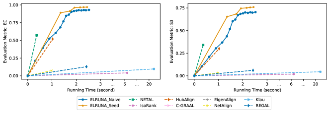
Figure 22: Quality-time comparison on bio_1 networks The last marker indicates the termination of the algorithm at which the algorithm is not improving any more. Each intermediate point indicates the termination of the algorithm at a particular iteration before convergence.

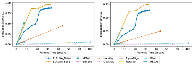
Figure 23: Quality-time comparison on bio_2 networks The last marker indicates the termination of the algorithm at which the algorithm is not improving any more. Each intermediate point indicates the termination of the algorithm at a particular iteration before convergence.

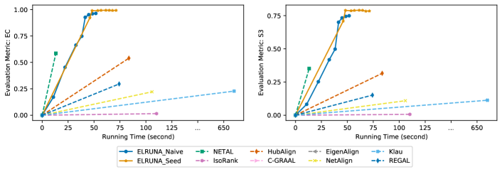
Figure 24: Quality-time comparison on erdos networks The last marker indicates the termination of the algorithm at which the algorithm is not improving any more. Each intermediate point indicates the termination of the algorithm at a particular iteration before convergence.

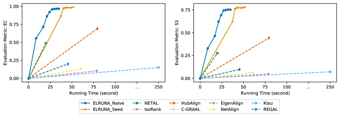
Figure 25: Quality-time comparison on retweet_1 networks The last marker indicates the termination of the algorithm at which the algorithm is not improving any more. Each intermediate point indicates the termination of the algorithm at a particular iteration before convergence.

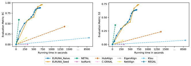
Figure 26: Quality-time comparison on social networks The last marker indicates the termination of the algorithm at which the algorithm is not improving any more. Each intermediate point indicates the termination of the algorithm at a particular iteration before convergence.

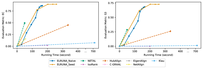
Figure 27: Quality-time comparison on digg networks The last marker indicates the termination of the algorithm at which the algorithm is not improving any more. Each intermediate point indicates the termination of the algorithm at a particular iteration before convergence.

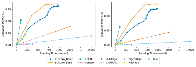
Figure 28: Quality-time comparison on facebook networks The last marker indicates the termination of the algorithm at which the algorithm is not improving any more. Each intermediate point indicates the termination of the algorithm at a particular iteration before convergence.

Result. As we have observed, in comparison with Klau and HubAlign, both versions of ELRUNA achieve significantly better alignment results with lower running time. Moreover, ELRUNA_Naive and ELRUNA_Seed always have intermediate states (at some $k$th iteration) that have running times similar to or lower than those of Netalign, REGAL, and IsoRank but produce much better results.

As for NETAL, we observe that ELRUNA_Naive always has an intermediate state with similar alignment quality and slightly higher running time. Also, ELRUNA_Seed always has an intermediate state with better alignment quality and slightly higher running time than those of NETAL. However, both proposed methods can further improve the alignment quality greatly beyond the intermediate state, whereas NETAL and other baselines cannot. In addition, as the two proposed algorithms proceed, each subsequent iteration always takes less time than the previous because the similarities are more defined after each iteration.

We observe that ELRUNA_Seed usually takes fewer iterations and longer running time to converge than does ELRUNA_Naive. These results are expected because the seed-and-extend alignment method is more computationally expensive than the naive alignment method.

5.3.2 Scalability

We evaluate the scalability of ELRUNA_Naive and ELRUNA_Seed by running them on networks from the self-alignment without and under noise testing case with no noisy edges. That is, we align $G_{1}$ with $G_{2}^{(0)}$. The result is shown in Figure 29.

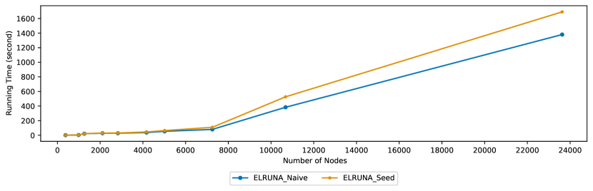
Figure 29: Scalability of ELRUNA

Results. We observe that the running time of both versions of ELRUNA is quadratic with respect to the number of nodes in networks.

5.4 Limitations: Alignment between Heterogeneous Networks

In this section, we discuss the limitations of ELRUNA. We compare ELRUNA with baselines on 5 pairs of networks where each pair consists of two networks from different domains. The first 3 pairs are social networks collected in  [38], and the other two pairs are biological networks [27]. The details of these networks are listed in Table 5.4.

tableDatasets for test case: Alignment between heterogeneous networks Doamin $n$ $m$ Offline vs Online 1,118 vs 3,906 1,511 vs 8,164 Flickr vs Lastfm 12,974 vs 15,436 16,149 vs 16,319 Flickr vs Myspace 6,714 vs 10,693 7,333 vs 10,686 Syne vs Yeast 1,837 vs 1,994 3,062 vs 15,819 Ecoli vs Yeast 1,274 vs 1,994 3,124 vs 15,819

In this experiment, we demonstrate the results without local search; that is, we show how ELRUNA outperforms the state-of-the-art methods. Results are shown in Figures 30–32. Because each pair of networks does not have underlying isomorphic subgraphs, the optimal objective is not known, and the highest EC is not 1.

We note that pairs of networks in this testing case do not have structurally similar underlying subgraphs. In fact, their topology could be very distinct from each other, given their different domains. Also, as we stated at the beginning of the experiment section, this comparison scenario is usually used by attributed network alignment algorithms. Therefore, it is not exactly what we solve with our formulation that relies solely on graph structure.

Results. We observe that ELRUNA_Naive did not perform well in this testing case due to the naive alignment method that it uses. As for ELRUNA_Seed, it achieves a 7.85% and a 11.41% increase in $EC$ over HubAlign and NETAL, respectively, for the pairs offline and online networks. Regarding other pairs of networks, the ELRUNA_Seed’s improvements of $EC$ HubAlign and NETAL are statistically insignificant. The results suggest that we need to enhance our algorithm in order to perform better under this testing case. One future direction is to extend ELRUNA to handle attributed networks.

Another limitation is that ELRUNA does not rely on the predefined vertex similarities; therefore, when such information is given, ELRUNA cannot utilize it to achieve better performance. For future work, we want to augment ELRUNA, which considers the prior similarities between vertices.

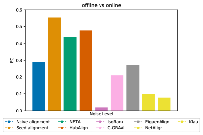
Figure 30: offline vs online networks

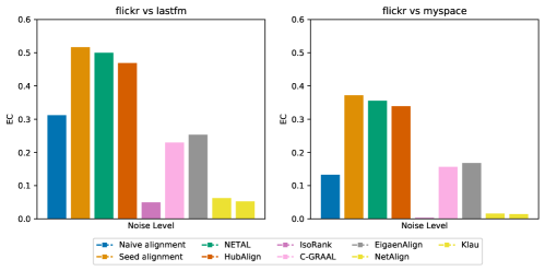
Figure 31: Flickr vs Lastfm and Flickr vs Myspace networks

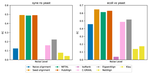
Figure 32: Syne vs Yeast and Ecoli vs Yeast networks

5.5 Evaluation of RAWSEM

In this section, we compare the performance of the proposed RAWSEM against the baseline local search. To evaluate their efficiency and effectiveness, we apply both methods as the postprocessing steps for ELRUNA_Naive. We align real-world networks from the self-alignment without and under noise testing case under the highest noise level. That is, $G_{1}$ is aligned with $G_{2}^{(0.25)}$. For each method we run it $20$ times on each pair of networks and measure its average running time, the average number of iterations to reach an optimum, and the average improved alignment quality. The results are summarized in Table 5.5.

Results. Clearly, RAWSEM outperforms the Baseline local search in terms of efficiency and effectiveness. In particular, RAWSEM achieves an increase of up to 13 times and 11 times for $EC$ and $S^{3}$, respectively, over the Baseline local search. Additionally, the number of iterations of the Baseline local search is orders of magnitude larger than that of RAWSEM. This experiment shows that RAWSEM can boost the alignment quality within seconds, thus making it a great candidate for a postprocessing step of network alignment algorithms.

We observe that RAWSEM does not always raise the objective to the global optima. This fact suggests that we should combine our selection rule with different local search methods, such as simulated annealing, to further enhance its performance. This is a further direction.

tableRAWSEM vs Baseline as postprosessing steps co-autho_1 bio_1 RAWSEM Baseline RAWSEM Baseline No. of iterations 1,301 28,091 1,817 32,274 Time (in seconds) 0.093 2.052 0.095 2.327 Improved $EC$ 2.3% 0.982% 3.231% 1.073% Improved $S^{3}$ 4.91% 1.175% 5.193% 1.91% econ router RAWSEM Baseline RAWSEM Baseline No. of iterations 1,580 50,000 798 42,367 Time (in seconds) 0.11 3.324 0.077 3.049 Improved $EC$ 0.506% 0% 1.406% 0.441% Improved $S^{3}$ 0.724% 0% 2.991% 0.892% bio_2 retweet_1 RAWSEM Baseline RAWSEM Baseline No. of iterations 3,069 61,290 4,415 60,272 Time (in seconds) 0.191 4.48 0.217 4.411 Improved $EC$ 5.477% 0.61% 1.241% 0.392% Improved $S^{3}$ 7.017% 1.326% 2.019% 0.673% erods retweet_2 RAWSEM Baseline RAWSEM Baseline No. of iterations 4,701 88,221 3,320 72,392 Time (in seconds) 0.323 6.25 0.204 5.19 Improved $EC$ 2.91% 0.31% 5.72% 0.437% Improved $S^{3}$ 4.801% 0.781% 10.08% 0.901% social google+ RAWSEM Baseline RAWSEM Baseline No. of iterations 7,701 100,297 11,928 152,116 Time (in seconds) 1.953 7.855 3.04 10.238 Improved $EC$ 4.903% 0.631% 3.29% 0.723% Improved $S^{3}$ 9.29% 1.01% 7.81% 1.59%

6 Conclusion and Future Work

In this paper, we propose ELRUNA, an iterative network alignment algorithm based on elimination rules. We also introduce RAWSEM, a novel random-walk-based selection rule for local search schemes that decreases the number of iterations needed to reach a local or global optimum. We conducted extensive experiments and demonstrate the superiority of ELRUNA and RAWSEM.

For future work, we aim to (1) improve the performance of ELRUNA on aligning regular graphs, (2) extend ELRUNA on aligning dense networks, and (3) develop advanced local search schemes to further reduce the number of iterations. Another possible extension of this work is to adopt the proposed algorithm to run on quantum computers as we have done in our previous work [28, 32, 30, 29].

Appendix

Pictorial examples of Rules 1 and 3

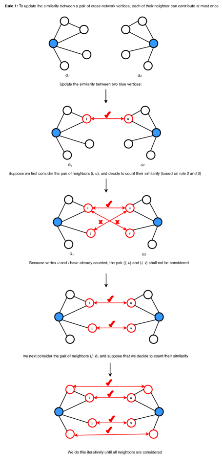
Figure 33: Rule 1 on an example graph

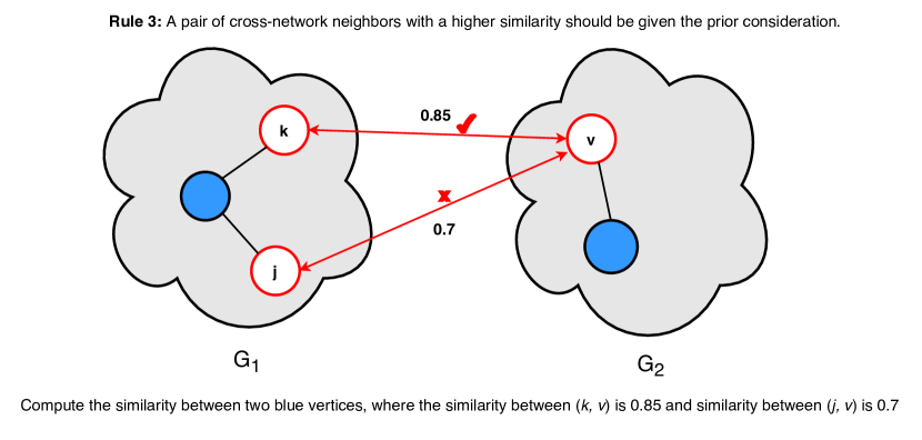
Figure 34: Rule 3 on an example graph

References

- [1] A. Barabási and R. Albert. Emergence of scaling in random networks. science, 286(5439):509–512, 1999.
- [2] M. Bayati, M. Gerritsen, D. Gleich, A. Saberi, and Y. Wang. Algorithms for large, sparse network alignment problems. In 2009 Ninth IEEE International Conference on Data Mining, pages 705–710, 2009.
- [3] Marián Boguná, Romualdo Pastor-Satorras, Albert Díaz-Guilera, and Alex Arenas. Models of social networks based on social distance attachment. Physical review E, 70(5):056122, 2004.
- [4] Munmun De Choudhury, Hari Sundaram, Ajita John, and Dorée Duncan Seligmann. Social synchrony: Predicting mimicry of user actions in online social media. In 2009 International conference on computational science and engineering, volume 4, pages 151–158. IEEE, 2009.
- [5] Boxin Du, Si Zhang, Nan Cao, and Hanghang Tong. First: Fast interactive attributed subgraph matching. In Proceedings of the 23rd ACM SIGKDD International Conference on Knowledge Discovery and Data Mining, pages 1447–1456, 2017.
- [6] Soheil Feizi, Gerald Quon, Mariana Mendoza, Muriel Medard, Manolis Kellis, and Ali Jadbabaie. Spectral alignment of graphs. IEEE Transactions on Network Science and Engineering, 2019.
- [7] P. Hiram Guzzi and T. Milenković. Survey of local and global biological network alignment: the need to reconcile the two sides of the same coin. Briefings in bioinformatics, 19(3):472–481, 2017.
- [8] S. Hashemifar, J. Ma, H. Naveed, S. Canzar, and J. Xu. ModuleAlign: module-based global alignment of protein–protein interaction networks. Bioinformatics, 32(17):i658–i664, 2016.
- [9] S. Hashemifar and J. Xu. Hubalign: an accurate and efficient method for global alignment of protein–protein interaction networks. Bioinformatics, 30(17):i438–i444, 2014.
- [10] Mark Heimann, Wei Lee, Shengjie Pan, Kuan-Yu Chen, and Danai Koutra. Hashalign: Hash-based alignment of multiple graphs. In Pacific-Asia Conference on Knowledge Discovery and Data Mining, pages 726–739. Springer, 2018.
- [11] Mark Heimann, Haoming Shen, Tara Safavi, and Danai Koutra. Regal: Representation learning-based graph alignment. In Proceedings of the 27th ACM International Conference on Information and Knowledge Management, pages 117–126, 2018.
- [12] P. Holme and B. Kim. Growing scale-free networks with tunable clustering. Physical review E, 65(2):026107, 2002.
- [13] G W. Klau. A new graph-based method for pairwise global network alignment. BMC bioinformatics, 10(1):S59, 2009.
- [14] D. Koutra, H. Tong, and D. Lubensky. Big-align: Fast bipartite graph alignment. In 2013 IEEE 13th ICDM, pages 389–398, 2013.
- [15] Danai Koutra and Christos Faloutsos. Individual and collective graph mining: principles, algorithms, and applications. Synthesis Lectures on Data Mining and Knowledge Discovery, 9(2):1–206, 2017.
- [16] Jure Leskovec and Julian J Mcauley. Learning to discover social circles in ego networks. In Advances in neural information processing systems, pages 539–547, 2012.
- [17] Chung-Shou Liao, Kanghao Lu, Michael Baym, Rohit Singh, and Bonnie Berger. IsoRankN: spectral methods for global alignment of multiple protein networks. Bioinformatics, 25(12):i253–i258, 2009.
- [18] Yangwei Liu, Hu Ding, Danyang Chen, and Jinhui Xu. Novel geometric approach for global alignment of PPI networks. In Thirty-First AAAI Conference on Artificial Intelligence, 2017.
- [19] Vesna Memišević and Nataša Pržulj. C-graal: Common-neighbors-based global graph alignment of biological networks. Integrative Biology, 4(7):734–743, 2012.
- [20] B. Neyshabur, A. Khadem, S. Hashemifar, and S. Arab. NETAL: a new graph-based method for global alignment of protein–protein interaction networks. Bioinformatics, 29(13):1654–1662, 2013.
- [21] Lawrence Page, Sergey Brin, Rajeev Motwani, and Terry Winograd. The pagerank citation ranking: Bringing order to the web. Technical report, Stanford InfoLab, 1999.
- [22] Rob Patro and Carl Kingsford. Global network alignment using multiscale spectral signatures. Bioinformatics, 28(23):3105–3114, 2012.
- [23] Dorit Ron, Ilya Safro, and Achi Brandt. Relaxation-based coarsening and multiscale graph organization. Multiscale Modeling & Simulation, 9(1):407–423, 2011.
- [24] Ryan A. Rossi and Nesreen K. Ahmed. An interactive data repository with visual analytics. SIGKDD Explor., 17(2):37–41, 2016.
- [25] Ilya Safro, Dorit Ron, and Achi Brandt. Graph minimum linear arrangement by multilevel weighted edge contractions. Journal of Algorithms, 60(1):24–41, 2006.
- [26] Ilya Safro, Peter Sanders, and Christian Schulz. Advanced coarsening schemes for graph partitioning. Journal of Experimental Algorithmics (JEA), 19:1–24, 2015.
- [27] Vikram Saraph and Tijana Milenković. MAGNA: maximizing accuracy in global network alignment. Bioinformatics, 30(20):2931–2940, 2014.
- [28] R. Shaydulin, H. Ushijima-Mwesigwa, I. Safro, S. Mniszewski, and Y. Alexeev. Community detection across emerging quantum architectures. arXiv preprint arXiv:1810.07765, 2018.
- [29] Ruslan Shaydulin, Hayato Ushijima-Mwesigwa, Christian FA Negre, Ilya Safro, Susan M Mniszewski, and Yuri Alexeev. A hybrid approach for solving optimization problems on small quantum computers. Computer, 52(6):18–26, 2019.
- [30] Ruslan Shaydulin, Hayato Ushijima-Mwesigwa, Ilya Safro, Susan Mniszewski, and Yuri Alexeev. Network community detection on small quantum computers. Advanced Quantum Technologies, page 1900029, 2019.
- [31] R. Singh, J. Xu, and B. Berger. Global alignment of multiple protein interaction networks with application to functional orthology detection. Proceedings of the National Academy of Sciences, 105(35):12763–12768, 2008.
- [32] Hayato Ushijima-Mwesigwa, Ruslan Shaydulin, Christian FA Negre, Susan M Mniszewski, Yuri Alexeev, and Ilya Safro. Multilevel combinatorial optimization across quantum architectures. arXiv preprint arXiv:1910.09985, 2019.
- [33] Vipin Vijayan, Dominic Critchlow, and Tijana Milenković. Alignment of dynamic networks. Bioinformatics, 33(14):i180–i189, 2017.
- [34] Vipin Vijayan, Vikram Saraph, and T Milenković. MAGNA++: Maximizing accuracy in global network alignment via both node and edge conservation. Bioinformatics, 31(14):2409–2411, 2015.
- [35] Bimal Viswanath, Alan Mislove, Meeyoung Cha, and Krishna P Gummadi. On the evolution of user interaction in Facebook. In Proceedings of the 2nd ACM workshop on Online social networks, pages 37–42, 2009.
- [36] J. Vogelstein, J. Conroy, V. Lyzinski, L. Podrazik, S. Kratzer, E. Harley, D. Fishkind, R. Vogelstein, and C. Priebe. Fast approximate quadratic programming for graph matching. PLOS one, 10(4):e0121002, 2015.
- [37] Abdurrahman Yasar and Ümit V Çatalyürek. An iterative global structure-assisted labeled network aligner. In Proceedings of the 24th ACM SIGKDD International Conference on Knowledge Discovery & Data Mining, pages 2614–2623, 2018.
- [38] S. Zhang and H. Tong. Final: Fast attributed network alignment. In Proceedings of the 22nd ACM SIGKDD, pages 1345–1354. ACM, 2016.
- [39] S. Zhang, H. Tong, R. Maciejewski, and T. Eliassi-Rad. Multilevel network alignment. In WWW, pages 2344–2354. ACM, 2019.