Generation of genuine tripartite entanglement for continuous variables in de Sitter space

Abstract

We study the distribution of quantum entanglement for continuous variables among causally disconnected open charts in de Sitter space. It is found that genuine tripartite entanglement is generated among the open chart modes under the influence of curvature of de Sitter space for any nonzero squeezing. Bipartite entanglement is also generated when the curvature is strong enough, even though the observers are separated by the event horizon. This provides a clearcut interpretation of the two-mode squeezing mechanism in the de Sitter space. In addition, the curvature generated genuine tripartite entanglement is found to be less sensitive to the mass parameter than the generated bipartite entanglement. The effects of the curvature of de Sitter space on the generated entanglement become more apparent in the limit of conformal and massless scalar fields.

I Introduction

Quantum entanglement, predicted by Schrödinger in 1935 schr , has fascinated many physicists since it was put forward due to its highly counterintuitive properties. As a central concept in quantum information theory, entanglement represents nonlocal correlation in quantum systems Bell . Entanglement is needed as key resource to carry out some quantum information processing tasks, e.g., quantum teleportation, quantum computation, quantum simulation, quantum superdense coding, quantum error correction, and so on Nielsen . It was recently realized that understanding the entanglement between field modes near a horizon, either black hole horizon or cosmic horizon, can help to understand some key questions in black hole thermodynamics and their relation to information Bombelli-Callen ; birelli ; Hawking-Terashima ; Brout . Therefore, many efforts have been expended on the investigation of entanglement in relativistic quantum systems Peres ; Schuller-Mann ; RQI1 ; jieci1 ; jieci2 ; Ralph ; RQI6 ; adesso2 ; RQI2 ; RQI4 ; RQI5 ; RQI7 ; adesso3 , and in the context of cosmology Ball:2005xa ; Fuentes:2010dt ; Nambu:2011ae ; Kanno16 ; wang2015 . In particular, we know that any two mutually separated regions would become causally disconnected in the exponentially expanding de Sitter space Sasaki:1994yt . The Bogoliubov transformations between the open chart vacua and the Bunch-Davies vacuum which have support on both regions of a free massive scalar field were derived in Sasaki:1994yt . Later, quantum entanglement and related nonlocal correlations of free field modes were studied in de Sitter space Maldacena:2012xp ; Albrecht18 ; Kanno:2014lma ; Kanno:2016qcc ; Choudhury:2017bou ; Iizuka:2014rua ; Nambu2018 ; Kanno:2014ifa ; Dimitrakopoulos:2015yva .

In this paper we study the distribution of quantum entanglement for continuous variables in de Sitter space. We consider the sharing of entanglement among three subsystems: the subsystem $A$ observed by a global observer Alice, the subsystem $B$ observed by Bob in region $R$ of the de Sitter space, and the subsystem $\bar{B}$ for an imaginary observer anti-Bob in region $L$. The initial state between modes $A$ and $B$ is prepared in a two-mode squeezed state from the perspective of a global observer. Our studying on the behaviors of continuous variables entanglement in de Sitter space is motivated by the following two reasons. Firstly, the two-mode squeezed state can be used to define particle states when the spacetime has at least two asymptotically flat regions birelli ; Peres ; Schuller-Mann ; Ralph ; adesso2 ; RQI2 ; RQI4 ; RQI5 ; adesso3 . This state has a special role in quantum field theory because the field modes in causally disconnected regions are found to be pair-wise squeezed due to spacetime evolution and relativistic effects birelli ; Peres ; Schuller-Mann ; Ralph ; adesso2 ; RQI2 ; RQI4 ; RQI5 ; adesso3 . Secondly, as a paradigmatic entangled state for continuous variables, the two-mode squeezed state can be produced in the lab and exploited for many current realization of continuous variable quantum information tasks brareview .

This work aims to study how the space curvature of de Sitter space affects the continuous variable entanglement described by observers in open chart vacua. We will derive the phase-space description of quantum state evolution in the de Sitter space basing on the Bogoliubov transformation between different open chart vacua and the Bunch-Davies vacuum. Then we evaluate not only the initial bipartite entanglement as degraded by the expanding de Sitter space, but remarkably, the multipartite entanglement which arises among all open chart modes. We are going to demonstrate that the bipartite entanglement initially prepared in the global bipartite modes does not disappear, but is redistributed among the modes in different open charts. As a consequence of the monogamy of entanglement, the entanglement between the initial modes described by the globe observers is degraded. In addition, the modes observed by Bob and anti-Bob are entangled when the curvature is strong enough even though they are separated by the event horizon, verifying the nonlocal nature of entanglement in curved space.

The outline of the paper is as follows. In Sec. II we review the solutions of mode functions and Bogoliubov transformations in the de Sitter space. In Sec. III we discuss the measurements of bipartite and tripartite Gaussian quantum entanglement. In Sec. IV we study the distribution of Gaussian quantum entanglement and the behaviors of the generated entanglement under the influences of the expanding and curvature of de Sitter space. The last section is devoted to a brief summary.

II Quantization of scalar field in de Sitter space

We consider a free scalar field $\phi$ with mass $m$ initially prepared in the Bunch-Davies vacuum of de Sitter space with metric $g_{\mu\nu}$. The action of the field is given by

$$S=\int d^{4}x\sqrt{-g}\left[\,-\frac{1}{2}\,g^{\mu\nu}\partial_{\mu}\phi\,\partial_{\nu}\phi-\frac{m^{2}}{2}\phi^{2}\,\right]\,.$$ (1)

Then we assume that one subsystem of the initial state is described the experimenter Bob who stays in the open region $R$ of the de Sitter space. The coordinate frames of open charts in de Sitter space can be obtained by analytic continuation from the Euclidean metric, and region $R$ is causally disconnected from region $L$ Sasaki:1994yt . The metrics for the open charts $R$ and $L$ in the de Sitter space are given by

$$ds^{2}_{R} = H^{-2}\left[-dt^{2}_{R}+\sinh^{2}t_{R}\left(dr^{2}_{R}+\sinh^{2}r_{R}\,d\Omega^{2}\right)\right]\,,$$

$$ds^{2}_{L} = H^{-2}\left[-dt^{2}_{L}+\sinh^{2}t_{L}\left(dr^{2}_{L}+\sinh^{2}r_{L}\,d\Omega^{2}\right)\right]\,,$$ (2)

where $H^{-1}$ is the Hubble radius and $d\Omega^{2}$ is the metric on the two-sphere.

Solving the Klein-Gordon equation for the scalar field $\phi$ in different open regions, one obtains

$$u_{\sigma p\ell m}(t_{R(L)},r_{R(L)},\Omega) \sim \frac{H}{\sinh t_{R(L)}}\,\chi_{p,\sigma}(t_{R(L)})\,Y_{p\ell m}(r_{R(L)},\Omega)\,,\qquad$$

$$-{\rm\bf L^{2}}Y_{p\ell m} = \left(1+p^{2}\right)Y_{p\ell m}\,,$$ (3)

where $Y_{p\ell m}$ are harmonic functions on the three-dimensional hyperbolic space. In Eq. (II) $\chi_{p,\sigma}(t_{R(L)})$ are positive frequency mode functions supporting on the $R$ and $L$ regions  Sasaki:1994yt

$$\chi_{p,\sigma}(t_{R(L)})=\left\{\begin{array}[]{l}\frac{e^{\pi p}-i\sigma e^{-i\pi\nu}}{\Gamma(\nu+ip+\frac{1}{2})}P_{\nu-\frac{1}{2}}^{ip}(\cosh t_{R})-\frac{e^{-\pi p}-i\sigma e^{-i\pi\nu}}{\Gamma(\nu-ip+\frac{1}{2})}P_{\nu-\frac{1}{2}}^{-ip}(\cosh t_{R})\,,\\ \\ \frac{\sigma e^{\pi p}-i\,e^{-i\pi\nu}}{\Gamma(\nu+ip+\frac{1}{2})}P_{\nu-\frac{1}{2}}^{ip}(\cosh t_{L})-\frac{\sigma e^{-\pi p}-i\,e^{-i\pi\nu}}{\Gamma(\nu-ip+\frac{1}{2})}P_{\nu-\frac{1}{2}}^{-ip}(\cosh t_{L})\,,\end{array}\right.$$ (7)

where $P^{\pm ip}_{\nu-\frac{1}{2}}$ are the associated Legendre functions and $\sigma=\pm 1$ is employed to distinguish the independent solutions in each open region. In addition, $p$ is a positive real parameter normalized by $H$, and $\nu$ is a mass parameter $\nu=\sqrt{\frac{9}{4}-\frac{m^{2}}{H^{2}}}\,$. These solutions can be normalized by the factor $N_{p}=\frac{4\sinh\pi p\,\sqrt{\cosh\pi p-\sigma\sin\pi\nu}}{\sqrt{\pi}\,|\Gamma(\nu+ip+\frac{1}{2})|}\,.$ To make the discussion clear we should know that $p$ can be regarded as the curvature parameter of the de Sitter space because, as $p$ becomes smaller than $1$, the effect of curvature gets stronger and stronger Kanno16 ; Albrecht18 . On the other hand , the mass parameter $\nu$ has two special values, which are $\nu=1/2$ for the conformally coupled massless scalar field and $\nu=3/2$ for the minimally coupled massless limit.

The scalar field can be expanded in terms of the creation and annihilation operators:

$$\hat{\phi}(t,r,\Omega)=\frac{H}{\sinh t}\int dp\sum_{\sigma,\ell,m}\left[\,a_{\sigma p\ell m}\,\chi_{p,\sigma}(t)+a_{\sigma p\ell-m}^{\dagger}\,\chi^{*}_{p,\sigma}(t)\right]Y_{p\ell m}(r,\Omega)\,,$$ (8)

where $a_{\sigma p\ell m}|0\rangle_{\rm BD}=0$ is the annihilation operator of the Bunch-Davies vacuum. For simplicity, hereafter we omit the indices $p$, $\ell$, $m$ in the operators $\phi_{p\ell m}$, $a_{\sigma p\ell m}$ and $a_{\sigma p\ell-m}^{\dagger}$. Similarly, the mode functions and the associated Legendre functions are rewritten as $\chi_{p,\sigma}(t)\rightarrow\chi^{\sigma}$, $P_{\nu-1/2}^{ip}(\cosh t_{R,L})\rightarrow P^{R,L}$, and $P_{\nu-1/2}^{-ip}(\cosh t_{R,L})\rightarrow P^{R*,L*}$.

On the other hand one can consider the positive frequency mode functions Sasaki:1994yt ; Kanno16 ; Albrecht18

$$\varphi^{q}=\left\{\begin{array}[]{ll}\frac{|\Gamma(1+ip)|}{\sqrt{2p}}P^{q}{}&\mbox{in region}~{}q\,,\\ 0{}&\mbox{in the opposite region}\,,\end{array}\right.$$ (11)

which are defined only on the $q=(R,L)$ region, respectively. In this case we introduce the creation and annihilation operators ($b_{q},b_{q}^{\dagger}$) in different regions by $b_{q}|0\rangle_{q}=0$. Then we can relate the creation and annihilation operators $(a_{\sigma},a_{\sigma}^{\dagger})$ and $(b_{q},b_{q}^{\dagger})$ in different reference frame by the Bogoliubov transformation

$$\phi(t)=a_{\sigma}\,\chi^{\sigma}+a_{\sigma}^{\dagger}\,\chi^{\sigma}{}^{*}=b_{q}\,\varphi^{q}+b_{q}^{\dagger}\,\varphi^{q}{}^{*}\,.$$ (12)

Using this transformation, the Bunch-Davies vacuum can be constructed from the vacuum states over $|0\rangle_{q}$ in the regions $R$ and $L$ Sasaki:1994yt ; Kanno16 ; Albrecht18 , which is

$$|0\rangle_{\rm BD}=N_{\gamma_{p}}^{-1}\exp\left(\gamma_{p}\,c_{R}^{\dagger}\,c_{L}^{\dagger}\,\right)|0\rangle_{R}|0\rangle_{L}\,,$$ (13)

where the parameter $\gamma_{p}$ is given by

$$\gamma_{p}=i\frac{\sqrt{2}}{\sqrt{\cosh 2\pi p+\cos 2\pi\nu}+\sqrt{\cosh 2\pi p+\cos 2\pi\nu+2}}\,.$$ (14)

The normalization factor $N_{\gamma_{p}}$ in Eq. (13) is found to be Sasaki:1994yt ; Kanno16 ; Albrecht18

$$N_{\gamma_{p}}^{2}=\left|\exp\left(\gamma_{p}\,c_{R}^{\dagger}\,c_{L}^{\dagger}\,\right)|0\rangle_{R}|0\rangle_{L}\right|^{2}=\frac{1}{1-|\gamma_{p}|^{2}}\,.$$ (15)

In addition, $\gamma_{p}$ simplifies to $|\gamma_{p}|=e^{-\pi p}$ for the conformally coupled massless scalar ($\nu=1/2$) and the minimally coupled massless scalar ($\nu=3/2$). It is worthy to note that the limit of large p has small $\gamma_{p}$ while small $p$ (i.e. larger curvature) has $\gamma_{p}$ approaching 1 ($\nu=1/2$). This because the effect of curvature becomes stronger and stronger when $p$ becomes smaller and smaller.

III Quantifying entanglement for continuous variables

In this section we recall the measures of Gaussian quantum entanglement for continuous variables. The character of a Gaussian state can be completely described in phase space by the symmetric covariance matrix $\bm{\sigma}$, whose entries are $\sigma_{ij}=\text{Tr}\big{[}{{{\{{{{\hat{R}}_{i}},{{\hat{R}}_{j}}}\}}_{+}}\ {\rho_{AB}}}\big{]}$. Here $\hat{R}=(\hat{x}_{1}^{A},\hat{p}_{1}^{A},\ldots,\hat{x}_{n}^{A},\hat{p}_{n}^{A},\hat{x}_{1}^{B},\hat{p}_{1}^{B},\ldots,\hat{x}_{m}^{B},\hat{p}_{m}^{B})^{\sf T}$ is a vector grouped the quadrature field operators. For each mode $i$, the phase space variables are defined by $\hat{a}_{i}^{A}=\frac{\hat{x}_{i}^{A}+i\hat{p}_{i}^{A}}{\sqrt{2}}$ and $\hat{a}_{i}^{B}=\frac{\hat{x}_{i}^{B}+i\hat{p}_{i}^{B}}{\sqrt{2}}$, where $\hat{a}_{i}^{A}$ and $\hat{a}_{i}^{B}$ are annihilation operators of the subsystems. The canonical commutation relations of these operators can be expressed as $[{{{\hat{R}}_{i}},{{\hat{R}}_{j}}}]=i{\Omega_{ij}}$, with the symplectic form $\Omega=\bigoplus_{1}^{n+m}{{\ 0\ \ 1}\choose{-1\ 0}}$. The covariance matrix $\sigma_{AB}$ must satisfy the Robertson-Schrödinger uncertainty relation simon87

$$\bm{\sigma}+i\Omega\geq 0\,,$$ (16)

to describe a physical state.

To measure bipartite entanglement in a relativistic setting, we employ the contangle contangle which is an entanglement monotone under Gaussian local operations and classical communication. This choice is because our main focus is the effect of spacetime curvature of de Sitter space on the distribution of entanglement among field modes in different open charts. In this setting, the contangle is the measure which enables mathematical treatment of distributed continuous variables entanglement as emerging from the fundamental monogamy constraints contangle ; hiroshima ; pisa . For pure states the contangle $\tau$ is defined as the square of the logarithmic negativity and it can be extended to mixed states by the Gaussian convex roof ordering . If $\bm{\sigma}_{AB}$ is the covariance matrix of a mixed bipartite Gaussian state where subsystem $A$ comprises one mode only, the contangle $\tau$ can be computed by (for detail please see Appendix A) contangle

$$\tau(\bm{\sigma}_{AB})\equiv\tau(\bm{\sigma}_{A|B}^{opt})=g[m_{AB}^{2}],\;\;\;g[x]={\rm arcsinh}^{2}[\sqrt{x-1}],$$ (17)

where $\bm{\sigma}_{AB}^{opt}$ corresponds to a pure Gaussian state, and $m_{AB}\equiv m(\bm{\sigma}_{AB}^{opt})=\sqrt{{\rm Det}\,\bm{\sigma}_{A}^{opt}}=\sqrt{{\rm Det}\,\bm{\sigma}_{B}^{opt}}$. The reduced covariance matrix $\bm{\sigma}_{A(B)}^{opt}$ of subsystem $A(B)$ are obtained by tracing over the degrees of freedom of subsystem $B$ ($A)$.

Unlike classical correlations, entanglement is monogamous, which means that it can not be freely shared among multiple subsystems of a mulitpartite quantum system pisa . Because of this property, we can employ the residual multipartite entanglement as a measurement of nonclassical correlations by exploring the entanglement distributed between multipartite systems. For a state distributed among $N$ parties each owns a single qubit (or a single mode), the monogamy constraint is described by the Coffman-Kundu-Wootters inequality ckw ,

$$E_{S_{i}|(S_{1}\ldots S_{i-1}S_{i+1}\ldots S_{N})}\geq\sum\limits_{j\neq i}^{N}{E_{S_{i}|S_{j}}},$$ (18)

where the multipartite system is partitioned in $N$ subsystems $S_{k}$ ($k=1,{\ldots},N$), each owning a single mode, and $E$ is the measure of bipartite entanglement between the $i$-th and $j$-th subsystems. The left hand side of inequality (18) measures the bipartite entanglement between a probe subsystem $S_{i}$ and the whole $N-1$ remaining subsystems. The other side quantifies the total bipartite entanglement between $S_{i}$ and each one of the remaining subsystems $S_{j\neq i}$ in the reduced subsystems. The residual multipartite entanglement is defined by the non-negative difference between these two entanglements, minimized over all choices of the probe subsystem.

In the simplest case of tripartite quantum system, the residual entanglement has the meaning of the genuine tripartite entanglement shared by the three subsystems ckw . In this case the multipartite entanglement is measured by contangle

$$\tau(\bm{\sigma}_{i|j|k})\equiv\min_{(i,j,k)}\left[\tau(\bm{\sigma}_{i|(jk)})-\tau(\bm{\sigma}_{i|j})-\tau(\bm{\sigma}_{i|k})\right]\,.$$ (19)

For pure states, the minimum in Eq. (19) is always attained by the decomposition realized with respect to the probe mode $i$ with smallest local determinant ${\rm Det}\,{\bm{\sigma}_{i}}=m^{2}_{i|(jk)}$ contangle .

IV Distribution of Gaussian entanglement in de Sitter space

IV.1 Generation of tripartite and bipartite Gaussian entanglement

As showed in Eq. (13), the Bunch-Davies vacuum for a global observer in de Sitter space can be expressed as a two-mode squeezed state of the $R$ and $L$ vacua Maldacena:2012xp ; Kanno:2014lma . Such state can be obtained by $|0\rangle_{\rm BD}=\hat{U}_{R,L}(\gamma_{p})|0\rangle_{R}|0\rangle_{L}$ in the Fock space, where $\hat{U}_{R,L}(\gamma_{p})=e^{\gamma_{p}(\hat{c}^{\dagger}_{\text{R}}\hat{c}^{\dagger}_{\text{L}}-\hat{c}_{\text{R}}\hat{c}_{\text{L}})}$ denotes the two-mode squeezing operator. In the phase space, the two-mode squeezing transformation can be expressed by the symplectic operator (for detail please see Appendix B)

$$S_{B,\bar{B}}(\gamma_{p})=\frac{1}{\sqrt{1-|\gamma_{p}|^{2}}}\left({\begin{array}[]{*{20}{c}}I_{2}&|\gamma_{p}|Z_{2}\\ |\gamma_{p}|Z_{2}&I_{2}\\ \end{array}}\right),$$ (22)

where the basics are $|kl\rangle=|k\rangle_{B}|l\rangle_{\bar{B}}$, which denotes that the squeezing transformation is acting on the modes observed by Bob and anti-Bob ($\bar{B}$). In this paper, we assume that Alice is a global observer who stays in the Bunch-Davies vacuum, while Bob is an observer resides in the region $R$ of the de Sitter open charts. We further assume that, there is no initial correlation between the entire state $\sigma^{\rm(G)}_{AB}(s)$ and the subsystem $\bar{B}$. Then the initial covariance matrix of the entire three mode state is $\sigma^{\rm(G)}_{AB}(s)\oplus I_{\bar{B}}$, where $\sigma^{\rm(G)}_{AB}(s)$ is prepared by an entangled Gaussian two-mode squeezed state in the Bunch-Davies vacuum

$$\sigma^{\rm(G)}_{AB}(s)=\left({\begin{array}[]{*{20}{c}}\cosh(2s)I_{2}&\sinh(2s)Z_{2}\\ \sinh(2s)Z_{2}&\cosh(2s)I_{2}\\ \end{array}}\right).$$ (25)

Here $I_{2}=\bigg{(}{\begin{array}[]{*{20}{c}}1&0\\ 0&1\\ \end{array}}\bigg{)}$, $Z_{2}=\bigg{(}\begin{array}[]{cc}1&0\\ 0&-1\\ \end{array}\bigg{)}$, and $s$ is the squeezing parameter. Under the transformation given in Eq. (22), the mode observed by Bob is mapped into two open charts. That is to say, an extra set of modes $\bar{B}$ becomes relevant from the perspective of Bob in the open chart $R$. Therefore, a complete description of the three mode state after the curvature-induced squeezing transformation is

$$\sigma^{\rm(a)}_{AB\bar{B}}(s,\gamma_{p}) = \big{[}I_{A}\oplus S_{B,\bar{B}}(\gamma_{p})\big{]}\big{[}\sigma^{\rm(G)}_{AB}(s)\oplus I_{\bar{B}}\big{]}$$ (26)

$$\big{[}I_{A}\oplus S_{B,\bar{B}}(\gamma_{p})\big{]}\,,$$

where $S_{B,\bar{B}}(\gamma_{p})$ is the phase-space expression of the two-mode squeezing in Eq. (22).

The genuine tripartite entanglement, as quantified by the residual contangle Eq. (19), is found to be

$$\tau_{(A|B|\bar{B})}=4s^{2}-{\rm arcsinh}^{2}\bigg{[}\sqrt{\frac{|\gamma_{p}|^{2}+(-2+|\gamma_{p}|^{2})\cosh(2s)}{\cosh(2s)|\gamma_{p}|^{2}+2-|\gamma_{p}|^{2}}-1}\bigg{]}\,.$$ (27)

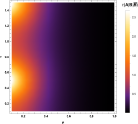
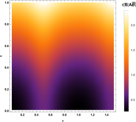
For any nonzero value of the squeezing parameters $s$ and $|\gamma_{p}|$, the residual contangle is nonzero. This in fact indicates that the state $\bm{\sigma}_{AB\bar{B}}$ is genuine entangled barbarella : it contains genuine tripartite entanglement among the global Alice, Bob in open chart $R$, and anti-Bob in open chart $L$. In Fig. (1 a), we plot the genuine tripartite entanglement $\tau_{(A|B|\bar{B})}$ as a function of the mass parameter $\nu$ and curvature parameter of de Sitter space $p$. The initial prepared entanglement in Bunch-Davies vacuum is kept fixed at $s=1.0$.

From Fig. (1 a) we can see that the genuine tripartite entanglement monotonically decrease with the increase of curvature parameter $p$. We know that the curvature of de Sitter space is a descending function of $p$ because, as $p$ is closer to zero, the effect of curvature gets stronger. Therefore, this in fact indicates that space curvature in de Sitter space generates genuine tripartite entanglement between the modes. Very remarkably, the genuine tripartite increases with increasing acceleration $\nu$ when $\nu<1/2$. It grows to a maximum for the conformally coupled massless scalar field ($\nu=1/2$) and then decreases. Again, we get the maximum value of the genuine tripartite entanglement when the mass parameter $\nu$ approaches the minimally coupled massless limit ( $\nu=3/2$). This generation of quantum entanglement will be precisely understood in the next subsection, where we will show that the initial prepared entanglement does not disappear, but is redistributed into tripartite correlations among different modes.

By using the definition Eq. (17), one can compute the bipartite contangles in different $1\to 2$ partitions of the state given in Eq. (26), which are found to be

$$\tau_{(A|B\bar{B})} = {\rm arcsinh}^{2}\bigg{[}\sqrt{\cosh(2s)-1}\bigg{]}\,,$$ (28)

$$\tau_{(B|A\bar{B})} = {\rm arcsinh}^{2}\bigg{[}\sqrt{\frac{\cosh(2s)+2|\gamma_{p}|^{2}-1}{1-|\gamma_{p}|^{2}}}\bigg{]}\,,$$

$$\tau_{(\bar{B}|AB)} = {\rm arcsinh}^{2}\bigg{[}\sqrt{\frac{|\gamma_{p}|^{2}(\cosh(2s)+1)}{1-|\gamma_{p}|^{2}}}\bigg{]}\,.$$

From Eq. (28) we can see that each single party is entangled with the block of the remaining two parties for any nonzero value of the parameters $s$ and $\gamma_{p}$, with respect to all possible global splitting of the three mode state.

Figure 1: (Color online). Gaussian quantum entanglement as a function of the mass parameter $\nu$ and curvature parameter of the de Sitter space $p$. The squeezing parameter $s$ in the initial state is fixed as $s=1$.

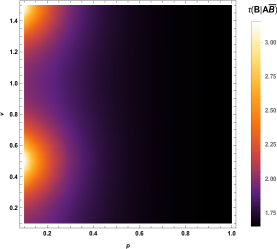
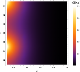
The values of the $1\to 2$ bipartite entanglement parameters from Eq. (28) are plotted in Fig. (1) as a function of the mass parameter $\nu$ and curvature parameter $p$, for a fixed degree of squeezing parameter $s=0.5$. From Fig. (1 b-c) we can see that the $1\to 2$ bipartite entanglement monotonically decrease with the increase of curvature parameter $p$, which means that space curvature also generates bipartite entanglement between these modes. However, the generated entanglement are apparently affected by the curvature of de Sitter space only around $\nu=1/2$ (conformal scalar limit) and $\nu=3/2$ (massless scalar limit). The degree of entanglement is much bigger than others when the value of $\nu$ is in the neighborhood of $\nu=1/2$ and $\nu=3/2$, as clearly visible in Fig. (1 b-c).

Figure 2: (Color online). Gaussian quantum entanglement as a function of the squeezing parameter $s$ and the mass parameter $\nu$. The curvature parameter of the de Sitter space is fixed as $p=0.2$.

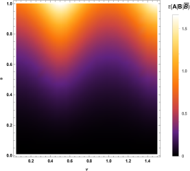
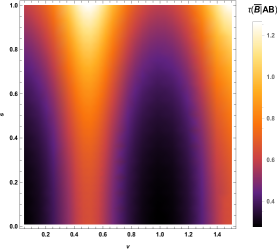
In Fig. (2 a), we plot the genuine tripartite entanglement $\tau_{(A|B|\bar{B})}$ as a function of the squeezing $s$ and mass parameter $\nu$ with fixed $p=0.2$. The bipartite quantum entanglement between the mode described by one observer and the group of modes described by the other two is plotted in Fig. (2 b-c). From (2 a-c) we can see that both the generated tripartite and bipartite are monotonous increasing function of the initial squeezing parameter $s$ in the Bunch-Davies vacuum. This confirms the fact that the distributed quantum resource in these mode root in the prepared resource in the two-mode squeezed state in Eq. (25). Due to the monogamy of entanglement, the entanglement between the initial modes is degraded. In addition, comparing to the bipartite contangles, the genuine tripartite entanglement $\tau_{(A|B|\bar{B})}$ is found to be less sensitive to the mass parameter $\nu$.

IV.2 Sharing of Gaussian entanglement among causally disconnected regions

To better understand the interplay between squeezing and the space curvature in the generation of Gaussian quantum entanglement, in this subsection we discuss the behavior of $1\to 1$ bipartite entanglement in the tripartite system. First of all, we find that there is no bipartite entanglement between the modes observed by the globe Alice and anti-Bob in the open chart $L$. Then we discuss the entanglement between the initial nonseparable Alice and Bob and the initial separable Bob and anti-Bob. Because Bob in chart $R$ has no access to the modes in the causally disconnected $L$ region, we must therefore trace over the inaccessible modes. Taking the trace over mode $\bar{B}$ in chart $L$, one obtains covariance matrix $\sigma_{AB}(s,\gamma_{p})$ for Alice and Bob

$$\sigma_{AB}(s,\gamma_{p})=\left({\begin{array}[]{*{20}{c}}\cosh(2s)I_{2}&\frac{\sinh(2s)}{\sqrt{1-|\gamma_{p}|^{2}}}Z_{2}\\ \frac{\sinh(2s)}{\sqrt{1-|\gamma_{p}|^{2}}}Z_{2}&\frac{|\gamma_{p}|^{2}+\cosh(2s)}{1-|\gamma_{p}|^{2}}I_{2}\\ \end{array}}\right).$$ (31)

We also interested in the Gaussian entanglement between mode $B$ in the $R$ region and anti-Bob in $L$ region, which are separated by the event horizon of the de Sitter space. Tracing over the modes in $A$, we obtain the covariance matrix $\sigma_{B\bar{B}}(s,\gamma_{p})$ for Bob and anti-Bob

$$\sigma_{B\bar{B}}(s,\gamma_{p})=\left({\begin{array}[]{*{20}{c}}\frac{|\gamma_{p}|^{2}+\cosh(2s)}{1-|\gamma_{p}|^{2}}I_{2}&\frac{2|\gamma_{p}|\cosh^{2}(s)}{1-|\gamma_{p}|^{2}}Z_{2}\\ \frac{2|\gamma_{p}|\cosh^{2}(s)}{1-|\gamma_{p}|^{2}}Z_{2}&\frac{1+|\gamma_{p}|^{2}\cosh(2s)}{1-|\gamma_{p}|^{2}}I_{2}\\ \end{array}}\right).$$ (34)

Then we find that the modes observed by Bob and anti-Bob are entangled when the curvature is strong enough even though they are separated by the event horizon, which verifies the fact that the entanglement is one kind of nonlocal quantum correlation.

Figure 3: (Color online). Bipartite entanglement between the modes as a function of the curvature parameter of the de Sitter space $p$. The initial squeezing parameter is fixed as $s=0.8$ and the mass parameter is fixed as $\nu=0.2$.

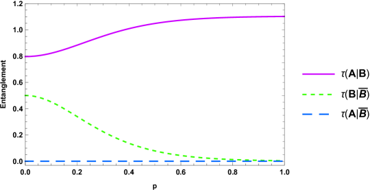
The contangles of the states $\sigma_{AB}$ and $\sigma_{B\bar{B}}$, quantifying the bipartite entanglement described by two observers, are found to be

$$\tau_{(A|B)} = {\rm arcsinh}^{2}\bigg{[}\frac{|\gamma_{p}|^{2}+(2-|\gamma_{p}|^{2})\cosh(2s)}{\cosh(2s)|\gamma_{p}|^{2}+2-|\gamma_{p}|^{2}}\bigg{]}\,,$$ (35)

$$\tau_{(B|\bar{B})} = {\rm arcsinh}^{2}\bigg{(}\frac{1+|\gamma_{p}|^{2}}{1-|\gamma_{p}|^{2}}\bigg{)}\,.$$ (36)

Let us give some comments on the quantum entanglement created between the modes in the open charts $R$ and $L$. Note that the entanglement in the mixed state $\bm{\sigma}_{B\bar{B}}$ is exactly equal to that of a pure two-mode squeezed state with squeezing $\gamma_{p}$. This provides a clearcut interpretation of the two-mode squeezing mechanism, in which the curvature of de Sitter space is responsible of the creation of entanglement between the accessible mode described by Bob, and the unaccessible one described by anti-Bob.

From Fig. (3) we can see that the bipartite entanglement between the initially entangled Alice and Bob monotonically increases with increasing $p$, while the entanglement between the causally disconnected Bob and anti-Bob decreases with increasing $p$. Now we have all the elements necessary to fully understand the spacetime curvature on Gaussian entanglement of scalar fields in the de Sitter space: There is bipartite entanglement between the two modes in the two distinct open charts, and this entanglement is a function of the spacetime curvature parameter. In addition, the bipartite entanglement initially prepared in the Bunch-Davies vacuum is redistributed into a genuine tripartite entanglement among the modes described by the observers in different open charts. Therefore, as a consequence of the monogamy of entanglement, the entanglement between the two modes $A$ and $B$ is degraded.

V Conclusions

We have studied the distribution of entanglement among the mode $A$ described by the globe observer Alice, mode $B$ described by Bob in the de Sitter region $R$, and the complimentary mode $\bar{B}$ described by a hypothetical observer anti-Bob in the causally disconnected region $L$. It is found that space curvature in de Sitter space generates genuine tripartite entanglement between the modes. In the expanding de Sitter space, each single party in the tripartite quantum system is entangled with the block of the remaining two parties, with respect to all possible global splitting of the three mode state. The modes $B$ and $\bar{B}$ get entangled when the curvature is strong enough even though they are separated by the event horizon. In addition, comparing to the generated bipartite entanglement, the generated genuine tripartite entanglement is found to be less sensitive to the mass parameter $\nu$. The modes observed by Bob and anti-Bob are entangled when the curvature is strong enough even though they are separated by the event horizon. This provides an interpretation of the two-mode squeezing mechanism, in which the curvature of de Sitter space is responsible of the creation of entanglement between them. We also find that the effects of the curvature of de Sitter space on the generated tripartite and bipartite entanglement become more apparent in the limit of conformal and massless scalar fields.

Appendix A The definition of contangle for continuous variables

In this appendix, we recall the definition of contangle for continuous variables and how it relates logarithmic negativity. Let us start with the monogamy inequality for a three mode Gaussian state

$$E^{i|(jk)}-E^{i|j}-E^{i|k}\geq 0\;,$$ (37)

where $E$ is a proper measure of bipartite entanglement and the indexes $\{i,j,k\}$ label the modes. When dealing with $1\times N$ partitions of a multimode pure Gaussian state together with its $1\times 1$ reduced partitions, the measure of entanglement should be a monotonically decreasing function $f(\tilde{n}_{-})$ of the smallest symplectic eigenvalue $\tilde{n}_{-}$ of the corresponding partially transposed covariance matrix $\tilde{\sigma}$. This is because $\tilde{n}_{-}$ is the only eigenvalue that can be smaller than $1$ adescaling , which violates the PPT criterion for the selected bipartition. Moreover, for a pure three mode Gaussian state, it is required that the bipartite entanglements $E^{i|(jk)}$ and $E^{i|j}=E^{i|k}$ are respectively functions $f(\tilde{n}_{-}^{i|(jk)})$ and $f(\tilde{n}_{-}^{i|j})$ of the associated smallest symplectic eigenvalues $\tilde{n}_{-}^{i|(jk)}$ and $\tilde{n}_{-}^{i|j}$ contangle .

For a generic pure state $|\psi\rangle$ of a $(1+N)$ mode continuous variable system, one can define the square of the logarithmic negativity as a measure of bipartite entanglement:

$$\tau(\psi)\equiv\ln^{2}\|\tilde{\rho}\|_{1}\;,\quad\rho=|\psi\rangle\!\langle\psi|\;.$$ (38)

This is a convex, increasing function of the logarithmic negativity $E_{\cal N}$. For any pure multipartite Gaussian state $|\psi\rangle$ with covariance matrix $\sigma$, explicit evaluation gives

$$\tau(\psi)\equiv\tau(\sigma)=\ln^{2}\left(1/\mu_{A}-\sqrt{1/\mu_{A}^{2}-1}\right),$$ (39)

where $\mu_{A}=1/\sqrt{{\rm Det}\,\sigma_{A}}$ is the local purity of the reduced covariance matrix $\sigma_{A}$. From Eq. (39) we can see that the convex roof of the squared logarithmic negativity defines the continuous-variable tangle, or, in short, the contangle for pure states contangle . The definition in Eq. (38) can be naturally extended to mixed states $\rho$ of $(N+1)$ mode continuous variable systems through the convex-roof formalism contangle . Namely, we can define the contangle $\tau(\rho)$ for mixed states as

$$\tau(\rho)\equiv\inf_{\{p_{i},\psi_{i}\}}\sum_{i}p_{i}\tau(\psi_{i})\;,$$ (40)

where the infimum is taken over all convex decompositions of $\rho$ in terms of pure states $\{|\psi_{i}\rangle\}$.

The sum in Eq. (40) should be replaced by an integral if the index $i$ is continuous, and the probabilities $\{p_{i}\}$ is replaced by the probability distribution $\pi(\sigma)$. For mixed multimode Gaussian states with covariance matrix $\sigma$, one should denote the contangle by $\tau(\sigma)$, in analogy with the notation used for pure Gaussian states. Then we define the contangle for Gaussian states by the infimum of the average contangle, taken over all pure Gaussian state,

$$\tau(\sigma)\equiv\inf_{\{\pi(d\sigma),\sigma\}}\int\pi(d\sigma)\tau(\sigma)\;.$$ (41)

If $\sigma_{AB}$ denotes a mixed two-mode Gaussian state, the Gaussian decomposition is the optimal one contangle , and the optimal pure state covariance matrix $\sigma_{AB}$ minimizing $\tau(\sigma_{AB})$ is characterized by $\tilde{n}_{-}(\tilde{\sigma_{AB}})$. Considering that the smallest symplectic eigenvalue is the same for both partially transposed covariance matrixes, we have $\tau(\sigma_{AB})=[\max\{0,-\ln\tilde{n}_{-}(\sigma_{AB})\}]^{2}$. Therefore, for a mixed bipartite Gaussian state where subsystem $A$ comprises one mode only, the contangle $\tau$ can be computed by contangle

$$\tau(\sigma_{AB})\equiv\tau(\sigma_{A|B}^{opt})=g[m_{AB}^{2}],\;\;\;g[x]={\rm arcsinh}^{2}[\sqrt{x-1}],$$ (42)

where $\sigma_{AB}^{opt}$ corresponds to a pure Gaussian state, and $m_{AB}\equiv m(\sigma_{AB}^{opt})=\sqrt{{\rm Det}\,\sigma_{A}^{opt}}=\sqrt{{\rm Det}\,\sigma_{B}^{opt}}$.

Appendix B Two-mode squeezed transformation in phase space and the entire final state

The Bunch-Davies vacuum for a global observer can be expressed as a two-mode squeezed state of the $R$ and $L$ vacua

$$|0\rangle_{\rm BD}=\sqrt{1-|\gamma_{p}|^{2}}\,\sum_{n=0}^{\infty}\gamma_{p}^{n}|n\rangle_{L}|n\rangle_{R}\,,$$ (43)

where $\gamma_{p}$ is the squeezing parameter. In the Fock space, the two-mode squeezed state can be obtained by $|0\rangle_{\rm BD}=\hat{U}_{R,L}(\gamma_{p})|0\rangle_{R}|0\rangle_{L}$, where $\hat{U}_{R,L}(\gamma_{p})=e^{\gamma_{p}(\hat{c}^{\dagger}_{\text{R}}\hat{c}^{\dagger}_{\text{L}}-\hat{c}_{\text{R}}\hat{c}_{\text{L}})}$ is the two mode squeezing operator. In the phase space, such transformation can be expressed by a symplectic phase-space operator

$$\sigma_{B\bar{B}}(\gamma_{p})=\begin{pmatrix}\cosh\left(2\gamma_{p}\right)&0&\sinh\left(2\gamma_{p}\right)&\sinh\left(2\gamma_{p}\right)\\ 0&\cosh\left(2\gamma_{p}\right)&\sinh\left(2\gamma_{p}\right)&-\sinh\left(2\gamma_{p}\right)\\ \sinh\left(2\gamma_{p}\right)&\sinh\left(2\gamma_{p}\right)&\cosh\left(2\gamma_{p}\right)&0\\ \sinh\left(2\gamma_{p}\right)&-\sinh\left(2\gamma_{p}\right)&0&\cosh\left(2\gamma_{p}\right)\end{pmatrix},$$ (44)

where $\cosh\gamma_{p}=(\sqrt{1-|\gamma_{p}|^{2}})^{-1}$. This covariance matrix is computed by $\sigma_{B\bar{B}}(\gamma_{p})=S^{T}_{B,\bar{B}}(\gamma_{p})I_{4}S_{B,\bar{B}}(\gamma_{p})$, where (Eq. 15 in the main manuscript)

$$S_{B,\bar{B}}(\gamma_{p})=\frac{1}{\sqrt{1-|\gamma_{p}|^{2}}}\left(\!\!\begin{array}[]{cccc}1&0&|\gamma_{p}|&0\\ 0&1&0&-|\gamma_{p}|\\ |\gamma_{p}|&0&1&0\\ 0&-|\gamma_{p}|&0&1\end{array}\!\!\right),$$ (49)

which denotes that squeezing transformation are performed to the bipartite state shared between Bob and anti-Bob ($\bar{B}$).

The expression given in Eq. (17) of the main manuscript is the phase space description of the entire state after the curvature-induced squeezing transformation given in Eq. (15). The covariance matrix of the entire state is computed by

$$\sigma_{AB\bar{B}}(s,r) = \big{[}I_{A}\oplus S_{B,\bar{B}}(\gamma_{p})\big{]}\big{[}\sigma^{\rm(M)}_{AB}(s)\oplus I_{\bar{B}}\big{]}$$ (53)

$$\big{[}I_{A}\oplus S_{B,\bar{B}}(\gamma_{p})\big{]}$$

$$= \left(\begin{array}[]{ccc}\mathcal{\sigma}_{A}&\mathcal{E}_{AB}&\mathcal{E}_{A\bar{B}}\\ \mathcal{E}^{\sf T}_{AB}&\mathcal{\sigma}_{B}&\mathcal{E}_{B\bar{B}}\\ \mathcal{E}^{\sf T}_{A\bar{B}}&\mathcal{E}^{\sf T}_{B\bar{B}}&\mathcal{\sigma}_{\bar{B}}\\ \end{array}\right)\,,$$

where $\sigma^{\rm(G)}_{AB}(s)\oplus I_{\bar{B}}$ is the initial covariance matrix for the entire system. In Eq. (26) the diagonal elements have the following forms:

$$\mathcal{\sigma}_{A}=\cosh(2s)I_{2},$$ (54)

$$\mathcal{\sigma}_{B}=[\cosh(2s)\cosh^{2}(\gamma_{p})+\sinh^{2}(\gamma_{p})]I_{2},$$ (55)

and

$$\mathcal{\sigma}_{\bar{B}}=[\cosh^{2}(\gamma_{p})+\cosh(2s)\sinh^{2}(\gamma_{p})]I_{2}.$$ (56)

The non-diagonal elements are $\mathcal{E}_{AB}=[\cosh(\gamma_{p})\sinh(2s)]Z_{2}$,

$$\mathcal{E}_{B\bar{B}}=[\cosh^{2}(s)\sinh(2\gamma_{p})]Z_{2},$$ (57)

and

$$\mathcal{E}_{A\bar{B}}=[\sinh(2s)\sinh(\gamma_{p})]Z_{2},$$ (58)

with

$$Z_{2}=\begin{pmatrix}1&0\\ 0&-1\end{pmatrix}.$$ (59)

References

- (1) E. Schrödinger, Proc. Camb. Phil. Soc. 31, 555 (1935).
- (2) J. Bell, On the Einstein Podolsky Rosen paradox, in Physics 1 (University of Maryland, College Park, MD, 1964), p. 195.
- (3) M. A. Nielsen and I. L. Chuang, Quantum Computation and Quantum Information (Cambridge University Press, Cambridge, England, 2000).
- (4) L. Bombelli, R. K. Koul, J. Lee, and R. Sorkin, Phys. Rev. D 34, 373 (1986).
- (5) S. W. Hawking, Commun. Math. Phys. 43, 199 (1975); Phys. Rev. D 14, 2460 (1976); H. Terashima, Phys. Rev. D 61, 104016 (2000).
- (6) R. Brout, S. Massar, R. Parentani, and P. Spindel, Phys. Rep. 260, 329 (1995).
- (7) N. D. Birrell and P. C. W. Davies, Quantum fields in curved space (Cambridge University Press,
- (8) A. Peres and D. R. Terno, Rev. Mod. Phys. 76, 93 (2004).
- (9) I. Fuentes-Schuller, and R. B. Mann, Phys. Rev. Lett. 95, 120404 (2005).
- (10) G. Adesso, I. Fuentes-Schuller, and M. Ericsson, Phys. Rev. A 76, 062112 (2007).
- (11) M. Aspachs, G. Adesso, and I. Fuentes, Phys. Rev. Lett 105, 151301 (2010).
- (12) D. J. Hosler, C. van de Bruck and P. Kok, Phys. Rev. A 85, 042312 (2012).
- (13) N. Friis, A. R. Lee, K. Truong, C. Sabín, E. Solano, G. Johansson, and I. Fuentes, Phys. Rev. Lett. 110, 113602 (2013).
- (14) J. Doukas, E. G. Brown, A. Dragan, and R. B. Mann, Phys. Rev. A 87, 012306 (2013).
- (15) D. Su, and T. C. Ralph, Phys. Rev. D 90, 084022 (2014).
- (16) J. Wang, H. Cao, J. Jing, and H. Fan, Phys. Rev. D 93, 125011 (2016).
- (17) T. Liu, J. Jing, and J. Wang, Adv. Quantum Technol. 1, 1800072 (2018); J. Wang, T. Liu, J. Jing, and S. Chen, Adv. Quantum Technol. 2, 1900003 (2019).
- (18) M. Ahmadi, D. E. Bruschi, and I. Fuentes, Phys. Rev. D 89, 065028 (2014); M. Ahmadi, A. R. H. Smith, and A. Dragan, Phys. Rev. A 92, 062319 (2015).
- (19) A. Blasco, L. J. Garay, M. Martín-Benito,and E. Martín-Martínez, Phys. Rev. Lett. 114, 141103 (2015).
- (20) B. Richter and Y. Omar, Phys. Rev. A 92, 022334 (2015).
- (21) J. L. Ball, I. Fuentes-Schuller and F. P. Schuller, Phys. Lett. A 359, 550 (2006).
- (22) I. Fuentes, R. B. Mann, E. Martin-Martinez and S. Moradi, Phys. Rev. D 82, 045030 (2010).
- (23) Y. Nambu and Y. Ohsumi, Phys. Rev. D 84, 044028 (2011).
- (24) J. Wang, Z. Tian, J. Jing, and H. Fan, Nucl. Phys. B 892, 390 (2015).
- (25) S. Kanno, J. P. Shock and J. Soda, Phys. Rev. D 94, 125014 (2016).
- (26) M. Sasaki, T. Tanaka and K. Yamamoto, Phys. Rev. D 51, 2979 (1995).
- (27) J. Maldacena and G. L. Pimentel, JHEP 1302, 038 (2013).
- (28) S. Kanno, J. Murugan, J. P. Shock and J. Soda, JHEP 1407, 072 (2014).
- (29) N. Iizuka, T. Noumi and N. Ogawa, Nucl. Phys. B 910, 23 (2016).
- (30) A. Albrecht, S. Kanno, and M. Sasaki, Phys. Rev. D 97, 083520 (2018).
- (31) A. Matsumura and Y. Nambu, Phys. Rev. D 98, 025004 (2018).
- (32) S. Kanno, M. Sasaki and T. Tanaka, JHEP 1703, 068 (2017).
- (33) S. Choudhury and S. Panda, Eur. Phys. J. C 78, 52 (2018).
- (34) S. Kanno, JCAP 1407, 029 (2014).
- (35) F. V. Dimitrakopoulos, L. Kabir, B. Mosk, M. Parikh and J. P. van der Schaar, JHEP 1506, 095 (2015).
- (36) S. L. Braunstein and P. van Loock, Rev. Mod. Phys. 77, 513 (2005).
- (37) R. Simon, E. C. G. Sudarshan, and N. Mukunda, Phys. Rev. A 36, 3868 (1987).
- (38) G. Adesso and F. Illuminati, New J. Phys. 8, 15 (2006).
- (39) T. Hiroshima, G. Adesso, and F. Illuminati, Phys. Rev. Lett. 98, 050503 (2007).
- (40) G. Adesso and F. Illuminati, Int. J. Quant. Info. 4, 383 (2006).
- (41) R. F. Werner and M. M. Wolf, Phys. Rev. Lett. 86, 3658 (2001).
- (42) G. Adesso, and F. Illuminati, Phys. Rev. A 72, 032334 (2005).
- (43) V. Coffman, J. Kundu, and W. K. Wootters, Phys. Rev. A 61, 052306 (2000).
- (44) G. Giedke, B. Kraus, M. Lewenstein, and J. I. Cirac, Phys. Rev. A 64, 052303 (2001).
- (45) G. Adesso, A. Serafini and F. Illuminati Phys. Rev. Lett. 93, 220504 (2004).