DNN Approximation of Nonlinear Finite Element Equations

Abstract.

We investigate the potential of applying (D)NN ((deep) neural networks) for approximating nonlinear mappings arising in the finite element discretization of nonlinear PDEs (partial differential equations). As an application, we apply the trained DNN to replace the coarse nonlinear operator thus avoiding the need to visit the fine level discretization in order to evaluate the actions of the true coarse nonlinear operator. The feasibility of the studied approach is demonstrated in a two-level FAS (full approximation scheme) used to solve a nonlinear diffusion-reaction PDE.

1. Introduction

In recent times deep neural networks, ([8]), have become the method of choice in solving state of the art machine learning problems, such as classification, clustering, pattern recognition, and prediction with enormous impact in many applied areas. There is also an increasing trend in scientific computing to take advantage of the potential of DNNs as nonlinear approximation tool, ([4]). This goes both for using DNNs in devising new approximation algorithms as well as for trying to develop mathematical theories that explain and quantify the ability of DNNs as universal approximation methodology, with results originating in ([6]) to many recent works, especially in the area of convolutional NN, ([16], [21], [7]). At any rate, this is still a very active area of research with no ultimate theoretical result available yet.

Recently, the deep neural networks have been also utilized in the field of numerical solution of PDEs ([1], [5], [9], [11], [12]), and for convolutional ones, see ([10]).

In this work, we investigate the ability of fully connected DNNs to provide an accurate enough approximation of the nonlinear mappings that arise in the finite element discretization of nonlinear PDEs. The finite element method applied to a nonlinear PDE posed variationally, basically requires the evaluation of integrals over each finite element which involves nonlinear functions that can be evaluated pointwise (generally, using quadratures). The unknown function $u_{h}$ which approximates the solution of the PDE is a linear combination of piecewise polynomials and the individual integrals for any given value of $u_{h}$ can be evaluated accurately enough (in general, approximately, using quadrature formulas). Typically, in a finite element discretization procedure, we use refinement. That is, we can have a fine enough final mesh, a set of elements ${\mathcal{T}}_{h}$, obtained from a previous level coarse mesh ${\mathcal{T}}_{H}$. One way to solve the fine-level nonlinear discretization problem, is to utilize the existing hierarchy of discretizations. One approach to maintain high accuracy of the coarse operators while evaluating their actions is to utilize the accurate fine level nonlinear operator. That is, for any given coarse finite element function, we expand it in terms of the fine level basis, apply the action of the fine level nonlinear operator and then restrict the result back to the coarse level, i.e., we apply a Galerkin procedure. This way of defining the coarse nonlinear operator provides better accuracy, however its evaluation requires fine-level computations. In the linear case, one can actually precompute the coarse level operators (matrices) explicitly, which is not the case in the nonlinear case. This study offers a way to generate a coarse operator, that can approximate the variationally defined finite element one on coarse levels by training a fully connected DNN. We do not do this globally, but rather construct the desired nonlinear mapping based on actions of locally trained DNNs associated with each coarse element from a coarse mesh ${\mathcal{T}}_{H}$. This is much more feasible than training the actions of the global coarse nonlinear mapping; these will have as input many coarse functions (i.e., their coefficient vectors) and are thus much bigger and hence much more expensive than their restrictions to the individual coarse elements.

The remainder of this paper is structured as follows. In Section 2, we introduce the problem in a general setting. Then in the following Section 2.3, we present a computational study of the training of the coarse nonlinear operators by varying the domain (a box in a high-dimensional space with size equal to the number of local coarse degrees of freedom). The purpose of the study is to assess the complexity of the local DNNs depending on the desired approximation accuracy. We also show the approximation accuracy of the global coarse nonlinear mapping (of our main interest) which depends on the coarsening ratio $H/h$. In Section 3, we introduce the FAS (full approximation scheme) solver ([2]), and in the following section 3.5, we apply the trained DNNs to replace the true coarse operator in a two-level FAS for a model nonlinear diffusion-reaction PDE discretized by piecewise linear elements. Finally, in Section 4, we draw some conclusions and outline few directions for possible future work.

2. Approximation for nonlinear mappings using DNNs

2.1. Problem setting

We are given the system of nonlinear equations

(2.1) $$F({\mathbf{u}})={\mathbf{f}}.$$

Here, $F$ is a mapping from ${\mathbb{R}}^{n}\mapsto{\mathbb{R}}^{n}$, and we have access only at its actions (by calling some function).

We assume that the solution belongs to a box $K\subset{\mathbb{R}}^{n}$, e.g., ${\mathbf{u}}\in[-a,a]^{n}$ for some value of $a>0$. Typically, nonlinear problems like (2.1) are solved by iterations, and for any given current iterate ${\mathbf{u}}$, we look for a correction ${\mathbf{g}}$ such that ${\mathbf{u}}:={\mathbf{u}}+{\mathbf{g}}$ gives a better accuracy. This motivates us to rewrite (2.1) as

$$G({\mathbf{u}},\;{\mathbf{g}})={\overline{\mathbf{f}}},$$

where

$$G({\mathbf{u}},\;{\mathbf{g}}):=F({\mathbf{u}}+{\mathbf{g}})-F({\mathbf{u}})\text{ and }{\overline{\mathbf{f}}}:={\mathbf{f}}-F({\mathbf{u}}).$$

Our goal is to train a DNN where ${\mathbf{u}}$ and ${\mathbf{g}}$ are the inputs and $G({\mathbf{u}},\;{\mathbf{g}})$ is the output. The input ${\mathbf{u}}$ is drawn from the box $K$, whereas the correction ${\mathbf{g}}$ is drawn from a small ball $B=\{\|{\mathbf{g}}\|\leq\delta\}$. In our study to follow, we vary the parameters $a$ and $\delta$ for a particular mapping $F$ (and respective $G$) to assess the complexity of the resulting DNN and examine the approximation accuracy. The general strategy is as follows. We draw $m_{a}\geq 1$ vectors from the box $K$ using Sobol sequence ([17, 18]) and $m_{\delta}\geq 1$ vectors from the ball $B$, also using Sobol sequence. The alternative would be to simply use random points in $K$ and $B$, however Sobol sequence is better in terms of cost versus approximation ability (at least for smooth mappings). Once we have built the DNN with a desired accuracy on the training data, we test its approximation quality on a number of randomly selected points from $K$ and $B$.

Our results are documented in the next subsection for a particular example of a finite element mapping; first on each individual subdomain (coarse element) $T\in{\mathcal{T}}_{H}$ and then for its global action composed from all locally trained DNNs.

2.2. Training DNNs for model nonlinear finite element mapping

We consider the nonlinear PDE

(2.2) $$\begin{array}[]{rl}-\text{div}(k(u)\nabla u)+u&=f\,\mbox{on}\,\Omega,\\ \nabla u\cdot\vec{n}&=0\,\mbox{on}\,\partial\Omega.\end{array}$$

Here, $\Omega$ is a polygon in ${\mathbb{R}}^{2}$ and $k(u)$ is a given positive nonlinear function of $u$.

The variational formulation for (2.2) is: find $u\in H^{1}(\Omega)$ such that

$$\int_{\Omega}(k(u)\nabla u\cdot\nabla v+uv)\;dx=\int_{\Omega}fv\;dx\,\mbox{for all}\,v\in H^{1}(\Omega).$$

The above problem is discretized by piecewise linear finite elements on triangular mesh ${\mathcal{T}}_{h}$ that yields a system of nonlinear equations.

In this section, we consider the coarse nonlinear mapping that corresponds to a coarse triangulation ${\mathcal{T}}_{H}$ which after refinement gives the fine one ${\mathcal{T}}_{h}$. The coarse finite element space is $V_{H}$ and the fine one is $V_{h}$. By construction, we have $V_{H}\subset V_{h}$. Let $\{\phi^{H}_{i}\}^{N_{H}}_{i=1}$ be the basis of $V_{H}$ and $\{\phi^{h}_{i}\}^{N_{h}}_{i=1}$ be the basis of $V_{h}$. These are piecewise linear functions associated with their respective triangulations ${\mathcal{T}}_{H}$ and ${\mathcal{T}}_{h}$. More specifically, we use Lagrangian bases, i.e., $\phi^{H}_{i}$ and $\phi^{h}_{i}$ are associated with the sets of vertices, ${\mathcal{N}}_{H}$ and ${\mathcal{N}}_{h}$, of the elements of their respective triangulations.

The coarse nonlinear operator $F:=F_{H}$ is then defined as follows. Let $u_{H}\in V_{H}$ be a coarse finite element function. Since $V_{H}\subset V_{h}$, we can expand $u_{H}$ in terms of the basis of $V_{h}$, i.e.,

$$u_{H}=\sum\limits_{{\mathbf{x}}_{i}\in{\mathcal{N}}_{h}}u_{H}({\mathbf{x}}_{i})\phi^{h}_{i}.$$

We can also expand $u_{H}$ in terms of the basis of $V_{H}$, i.e., we have

$$u_{H}=\sum\limits_{{\mathbf{x}}_{i}\in{\mathcal{N}}_{H}}u_{H}({\mathbf{x}}_{i})\phi^{H}_{i}.$$

In the actual computations we use their coefficient vectors

$${\mathbf{u}}_{c}=(u_{H}({\mathbf{x}}_{i}))_{{\mathbf{x}}_{i}\in{\mathcal{N}}_{H}}\in{\mathbb{R}}^{N_{H}}\text{ and }{\mathbf{u}}=(u_{H}({\mathbf{x}}_{i}))_{{\mathbf{x}}_{i}\in{\mathcal{N}}_{h}}\in{\mathbb{R}}^{N_{h}}.$$

These coefficient vectors are related by an interpolation mapping $P$ (which is piecewise linear), i.e., we have

$${\mathbf{u}}=P{\mathbf{u}}_{c}.$$

First we define the local nonlinear mappings $F:=F^{H}_{T}$, associated with each $T\in{\mathcal{T}}_{H}$.

In terms of finite element functions, we have as input $u_{H}$ restricted to $T$, and we evaluate the integrals

$$F^{H}_{T}:\;\left.u_{H}\right|_{T}\mapsto\int\limits_{T}k(u_{H})\nabla u_{H}\cdot\nabla\phi^{H}_{i}\;d{\mathbf{x}},\text{ for all vertices }{\mathbf{x}}_{i}\text{ of the coarse element }T.$$

Each integral over $T$ is computed as a sum of integrals over the fine-level elements $\tau\subset T$, $\tau\in{\mathcal{T}}_{h}$, using fine level computations, i.e., $u_{H}$ and $\phi^{H}_{i}$ are linear on each $\tau$ and these fine-level integrals are assumed computable (by the finite element software used to generate the fine level discretization, which possibly employs high order quadratures).

In terms of linear algebra computations, we have ${\mathbf{u}}_{c,\;T}=(u^{H}({\mathbf{x}}_{i}))_{{\mathbf{x}}_{i}\in{\mathcal{N}}_{H}\cap T}$ as an input vector, and have as an output a vector $F^{H}_{T}({\mathbf{u}}_{c,\;T})$ of the same size, i.e., equal to the number of vertices of $T$. Note that we will be training the DNN for the mapping of two variables, ${\mathbf{u}}_{c,\;T}$ and ${\mathbf{g}}_{c,\>T}$, i.e.,

$$G_{T}({\mathbf{u}}_{c,\;T},\;{\mathbf{g}}_{c,\;T}):=F^{H}_{T}({\mathbf{u}}_{c,\;T}+{\mathbf{g}}_{c,\;T})-F^{H}_{T}({\mathbf{u}}_{c,\;T}).$$

That is, the input vectors will have size two times bigger than the output vectors. Once we have trained the local actions of the nonlinear mapping, the global action is obtained by standard assembly, using the fact that

(2.3) $$G({\mathbf{u}}_{c},\;{\mathbf{g}}_{c})=\sum\limits_{T\in{\mathcal{T}}_{H}}I_{T}G_{T}({\mathbf{u}}_{c,\;T},\;{\mathbf{g}}_{c,\;T}).$$

Here, $I_{T}$ stands for the mapping that extends a local vector defined on $T$ to a global vector by zero values outside $T$. For a global vector ${\mathbf{v}}_{c}$, ${\mathbf{v}}_{c,\;T}=(I_{T})^{T}{\mathbf{v}}_{c}=\left.{\mathbf{v}}_{c}\right|_{T}$ denotes its restriction to $T$.

In the following section, we provide actual test results for training DNNs, first for the local mappings $G_{T}$, and then for the respective global one $G$.

2.3. Training local DNNs for the model finite element mapping

We use Keras, ([14]), a Python Deep Learning library to approximate nonlinear mappings. Keras is a high-level neural networks API (Application Programming Interface), written in Python and capable of running on top of TensorFlow ([15]). In this work, we use a fully connected network. The Sequential model in Keras provides a way to implement such a network.

The input vectors are of size $2n_{c}$ (${\mathbf{u}}_{c,T}$ stacked on top of ${\mathbf{g}}_{c,T}$) and the desired outputs are the actions ($G_{T}({\mathbf{u}}_{c,T},\;{\mathbf{g}}_{c,T})$) represented as vectors of size $n_{c}$ for any given input. The network consists of few fully connected layers with tanh activation at each layer. We use the standard mean squared error as the loss function.

In the tests to follow, we use data ${\mathbf{u}}_{c,\;T}$ from the boxes $K$, and ${\mathbf{g}}_{c,T}$ from balls $B$ of various sizes. Specifically, we performed the numerical tests with $10$ ${\mathbf{u}}_{c,\;T}$ vectors each taken from

$$K=[-1,1]^{n_{c}},[-0.1,0.1]^{n_{c}},[-0.05,0.05]^{n_{c}},[-0.01,0.01]^{n_{c}},$$

and $50$ ${\mathbf{g}}_{c,\;T}$ vectors drawn from balls $B$ with radii $\delta_{B}=0.1,0.05,0.01,0.005$, respectively (i.e., the first $K$ is paired with the first ball $B$, the second box $K$ is paired with the second ball $B$, and so on). In our test we have chosen $n_{c}=4$, that is, the local sets $T$ have four coarse dofs. Also, we vary the ratio $H/h=2,4,8$, which implies that we have $9,16,$ and $81$ fine dofs, respectively (while keeping fixed the number of coarse dofs $n_{c}=4$ in $T$).

The network was trained with $3$ layers, each with $16$ neurons. The training algorithm was provided by TensorFlow using the ADAM optimizer ([13]) which is a variant of the SGD (stochastic gradient descent) algorithm, see, e.g., ([19]). We used $500$ epochs, $batch\,size=10$, learning rate $\alpha=0.001$ along with $\beta_{1}=0.9$ and $\beta_{2}=0.999$. For more details on the meaning of these parameters, we refer to ([14]) and ([19]).

figureSchematic representation of the used network architecture

Let $G_{T_{DNN}}$ be the action after the training. Tables 2.3, 2.3, and 2.3 show the average of the relative errors using $\left\|\right\|_{2}$ and $\left\|\right\|_{\infty}$ of $\dfrac{\left\|G_{T}({\mathbf{u}}_{c,\;T},\;{\mathbf{g}}_{c,\;T})-G_{T_{DNN}}({\mathbf{u}}_{c,\;T},\;{\mathbf{g}}_{c,\;T})\right\|_{2}}{\left\|G_{T}({\mathbf{u}}_{c,\;T},\;{\mathbf{g}}_{c,\;T})\right\|_{2}}$ and $\dfrac{\left\|G_{T}({\mathbf{u}}_{c,\;T},\;{\mathbf{g}}_{c,\;T})-G_{T_{DNN}}({\mathbf{u}}_{c,\;T},\;{\mathbf{g}}_{c,\;T})\right\|_{\infty}}{\left\|G_{T}({\mathbf{u}}_{c,\;T},\;{\mathbf{g}}_{c,\;T})\right\|_{\infty}}$ over $100$ examples consisting of $10$ ${\mathbf{u}}_{c,\;T}$ within the box $K$ and $10$ ${\mathbf{g}}_{c,\;T}$ within the ball $B$.

$K$	$\delta_{B}$	relative $\ell_{2}$-error	relative $\ell_{\infty}$-error
$[-1,1]^{n_{c}}$	0.1	0.005209	0.007234
$[-1,1]^{n_{c}}$	0.05	0.000829	0.001168
$[-1,1]^{n_{c}}$	0.01	0.000245	0.000374
$[-1,1]^{n_{c}}$	0.005	0.000125	0.000193
$[-0.1,0.1]^{n_{c}}$	0.05	0.000131	0.000186
$[-0.1,0.1]^{n_{c}}$	0.01	3.858919E-06	5.973702E-06
$[-0.1,0.1]^{n_{c}}$	0.005	3.966236E-06	6.276684E-06
$[-0.05,0.05]^{n_{c}}$	0.01	1.043632E-06	1.487640E-06
$[-0.05,0.05]^{n_{c}}$	0.005	6.841004E-07	1.048721E-06
$[-0.01,0.01]^{n_{c}}$	0.005	3.636231E-08	5.151947E-08

tableThe relative average $L_{2}$ and $L_{\infty}$ errors for $H/h=2$

$K$	$\delta_{B}$	relative $\ell_{2}$-error	relative $\ell_{\infty}$-error
$[-1,1]^{n_{c}}$	0.1	0.001198	0.001670
$[-1,1]^{n_{c}}$	0.05	0.0007022	0.001021
$[-1,1]^{n_{c}}$	0.01	0.000254	0.000377
$[-1,1]^{n_{c}}$	0.005	1.692172E-05	2.455399E-05
$[-0.1,0.1]^{n_{c}}$	0.05	1.692172E-05	2.455399E-05
$[-0.1,0.1]^{n_{c}}$	0.01	3.105803E-06	4.837250E-06
$[-0.1,0.1]^{n_{c}}$	0.005	2.251858E-06	3.573355E-06
$[-0.05,0.05]^{n_{c}}$	0.01	8.565291E-07	1.322711E-06
$[-0.05,0.05]^{n_{c}}$	0.005	6.394531E-07	9.717701E-07
$[-0.01,0.01]^{n_{c}}$	0.005	2.872041E-08	4.041187E-08

tableThe relative average $L_{2}$ and $L_{\infty}$ errors for $H/h=4$

$K$	$\delta_{B}$	relative $\ell_{2}$-error	relative $\ell_{\infty}$-error
$[-1,1]^{n_{c}}$	0.1	0.001060	0.001010
$[-1,1]^{n_{c}}$	0.05	0.000641	0.001003
$[-1,1]^{n_{c}}$	0.01	0.000196	0.000292
$[-1,1]^{n_{c}}$	0.005	1.141443E-05	1.723346E-05
$[-0.1,0.1]^{n_{c}}$	0.05	1.151866E-05	1.744020E-05
$[-0.1,0.1]^{n_{c}}$	0.01	2.756513E-06	4.175218E-06
$[-0.1,0.1]^{n_{c}}$	0.005	2.115907E-06	3.441013E-06
$[-0.05,0.05]^{n_{c}}$	0.01	8.378942E-07	1.221053E-06
$[-0.05,0.05]^{n_{c}}$	0.005	5.626164E-07	8.913452E-07
$[-0.01,0.01]^{n_{c}}$	0.005	2.645869E-08	3.999300E-08

tableThe relative average $L_{2}$ and $L_{\infty}$ errors for $H/h=8$

The approximation of the global coarse nonlinear operator is presented in Table 2.3. As it is seen from formula (2.3), we can approximate each $G_{T}$ independently of each other, and after combining the individual approximations (using the same assembly formula with each $G_{T}$ replaced by its DNN approximation), we define the approximation to the global $G$. We use the same setting for training the individual neural networks for each $G_{T}$. We have decomposed $\Omega$ into several subdomains $T\in{\mathcal{T}}_{H}$ so that which each $T$ has $n_{c}=4$. In this test, we chose $H/h=2$.

In Table 2.3, we show how the accuracy varies for different local boxes $K$ and respective balls $B$. As before, we present the average of the relative $L_{2}$ and $L_{\infty}$ errors. One can notice that for finer $h$ (and $H=2h$), i.e., more local subdomains $T$, we get somewhat better approximations of the global $G$. It should be expected since  with smaller $h$ the finite element problem approximates better the continuous one. Some visual illustration of this fact is presented in Figures 1, 2, 3, 4, 5, and 6. More specifically, we provide plots of $G_{T}$ and $G_{T_{DNN}}$ for the data that achieves the min and max $L_{2}$ errors when the number of subdomains are 4, 16 and 64 corersponding to box $K=[-0.05,0.05]$ and and ball $B$ with $\delta_{B}=0.005$.

# of subdomains	$K=[-1,1]$	$K=[-0.1,0.1]$	$K=[-0.05,0.05]$
	$\delta_{B}=0.1$	$\delta_{B}=0.01$	$\delta_{B}=0.005$
4	$L_{2}\,\mbox{error:}\,$0.004838	6.379939E-05	9.578247E-06
	$L_{\infty}\,\mbox{error:}\,$ 0.008154	0.000130	3.154789E-05
16	$L_{2}\,\mbox{error:}\,$0.003847	4.363349E-05	1.112007E-06
	$L_{\infty}\,\mbox{error:}\,$ 0.005229	0.000021	1.828478E-05
64	$L_{2}\,\mbox{error:}\,$0.002977	7.388419E-06	8.997734E-07
	$L_{\infty}\,\mbox{error:}\,$ 0.003401	2.789513e-5	3.907758E-06
100	$L_{2}\,\mbox{error:}\,$: 0.000909	5.655502e-6	9.043519E-08
	$L_{\infty}\,\mbox{error:}\,$ 0.001688	1.542110e-5	4.098461E-07

tableComparison for different numbers of subdomains

For the next test, we have $n_{c}=4$ and $H/h=4$. The same settings for neural networks are used along with $K=[-0.05,0.05]$ and $\delta_{B}=0.005$. The results in Table 2.3 show the average of the relative $L_{2}$ and $L_{\infty}$ errors for different number of subdomains.

# of subdomains	$L_{2}$ min	$L_{2}$ max	$L_{2}$	$L_{\infty}$
4	2.204530E-06	1.012479E-04	5.276626E-06	2.367189E-05
16	1.307212E-07	2.768105E-05	7.107769E-07	2.068912E-06
64	4.8551896E-08	1.395091E-05	5.341155E-08	7.789968E-07

tableThe relative average $L_{2}$ and $L_{\infty}$ errors for $H/h=4$

As expected, since smaller $h$ and fixed $H$ gives better approximation of the nonlinear operator, for the ratio $H/h=4$ we do see better approximation than for $H/h=2$.

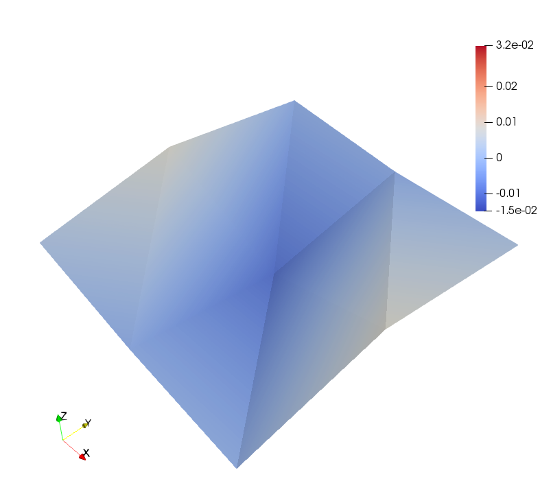
(a) $G_{T}({\mathbf{u}}_{c,\;T},\;{\mathbf{g}}_{c,\;T})$

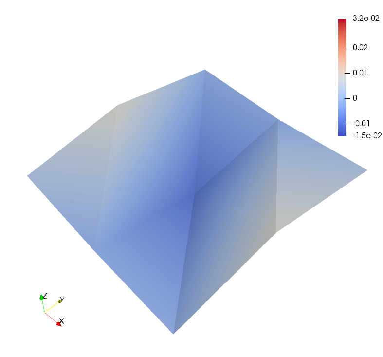
(b) $G_{T_{DNN}}({\mathbf{u}}_{c,\;T},\;{\mathbf{g}}_{c,\;T})$

Figure 1. Plots of $G_{T}$ and $G_{T_{DNN},\;{\mathbf{g}}_{c,\;T}}$ for four subdomains at the $({\mathbf{u}}_{c,\;T},\;{\mathbf{g}}_{c,\;T})$ which achieves the min $L_{2}$ error. The min relative error is $2.662757E{-06}$.

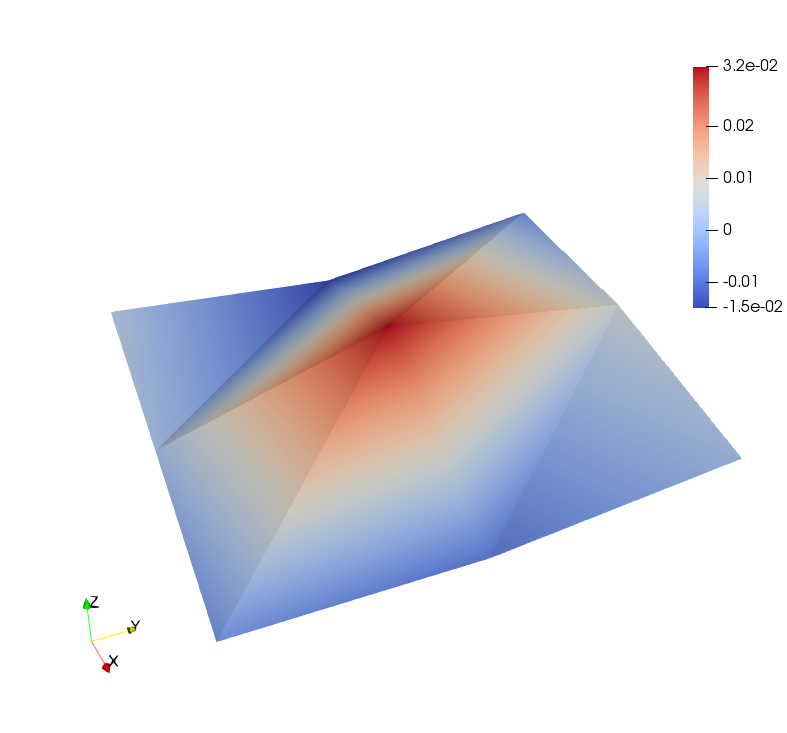
(a) $G_{T}({\mathbf{u}}_{c,\;T},\;{\mathbf{g}}_{c,\;T})$

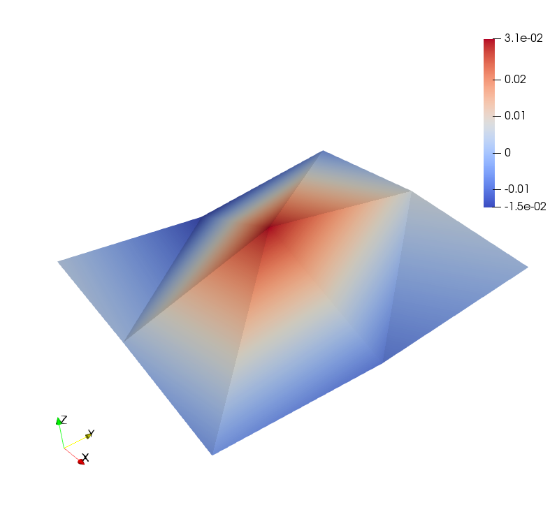
(b) $G_{T_{DNN}}({\mathbf{u}}_{c,\;T},\;{\mathbf{g}}_{c,\;T})$

Figure 2. Plots of $G_{T}$ and $G_{T_{DNN}}$ for four subdomains at the $({\mathbf{u}}_{c,\;T},\;{\mathbf{g}}_{c,\;T})$ which achieves the max $L_{2}$ error. The max relative error is $1.122974E{-04}$.

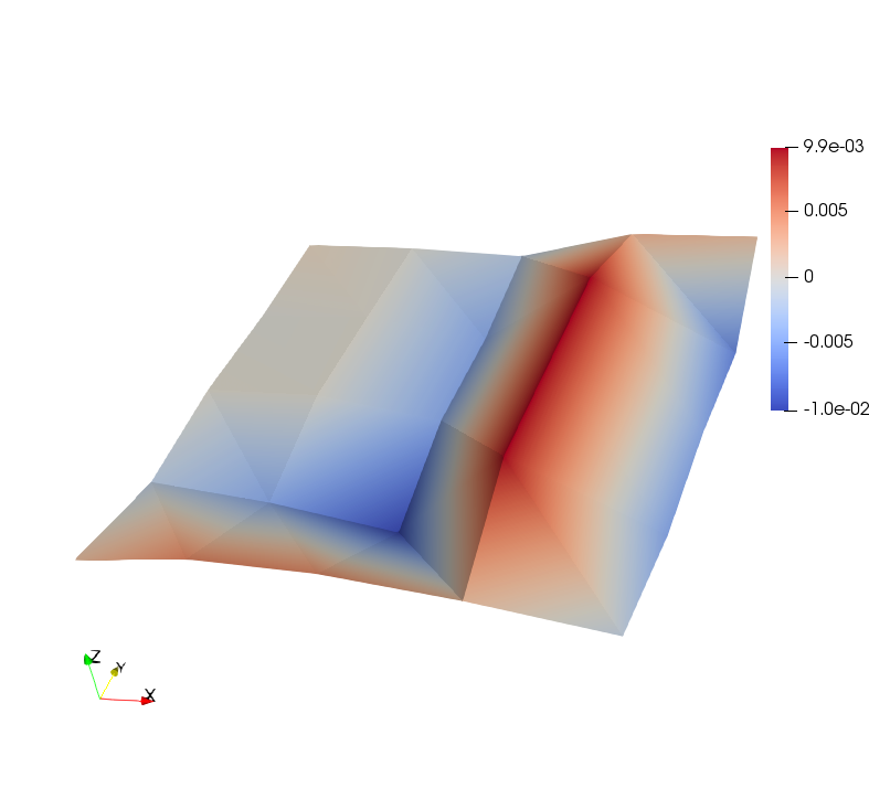
(a) $G_{T}({\mathbf{u}}_{c,\;T},\;{\mathbf{g}}_{c,\;T})$

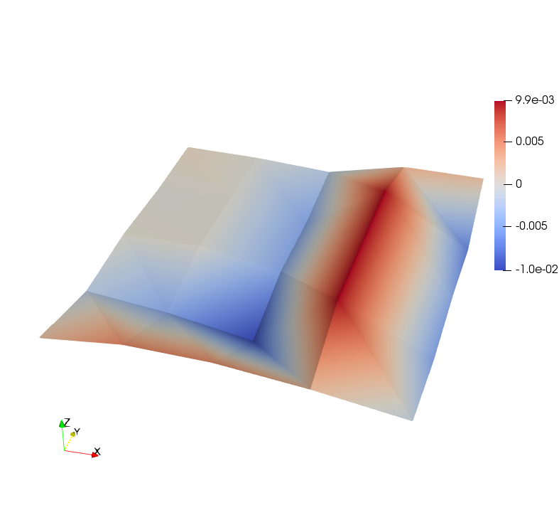
(b) $G_{T_{DNN}}({\mathbf{u}}_{c,\;T},\;{\mathbf{g}}_{c,\;T})$

Figure 3. Plots of $G_{T}$ and $G_{T_{DNN}}$ for sixteen subdomains at the $({\mathbf{u}}_{c,\;T},\;{\mathbf{g}}_{c,\;T})$ which achieves the min $L_{2}$ error. The min relative error is $8.886265E{-07}$.

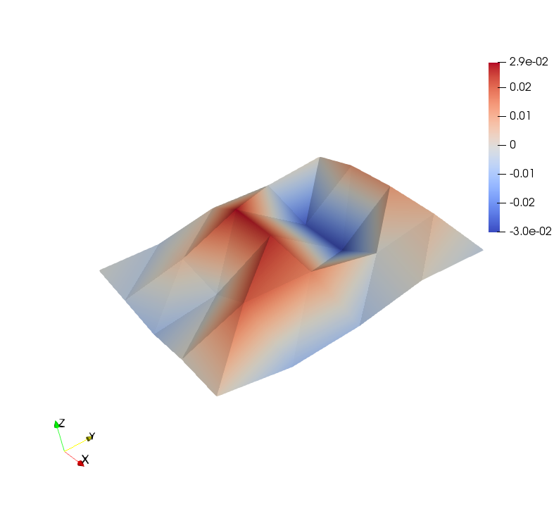
(a) $G_{T}({\mathbf{u}}_{c,\;T},\;{\mathbf{g}}_{c,\;T})$

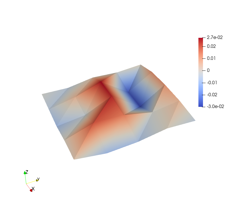
(b) $G_{T_{DNN}}({\mathbf{u}}_{c,\;T},\;{\mathbf{g}}_{c,\;T})$

Figure 4. Plots of $G_{T}$ and $G_{T_{DNN}}$ for sixteen subdomains at the $({\mathbf{u}}_{c,\;T},\;{\mathbf{g}}_{c,\;T})$ which achieves the max $L_{2}$ error. The max relative error is $1.285776E{-05}$.

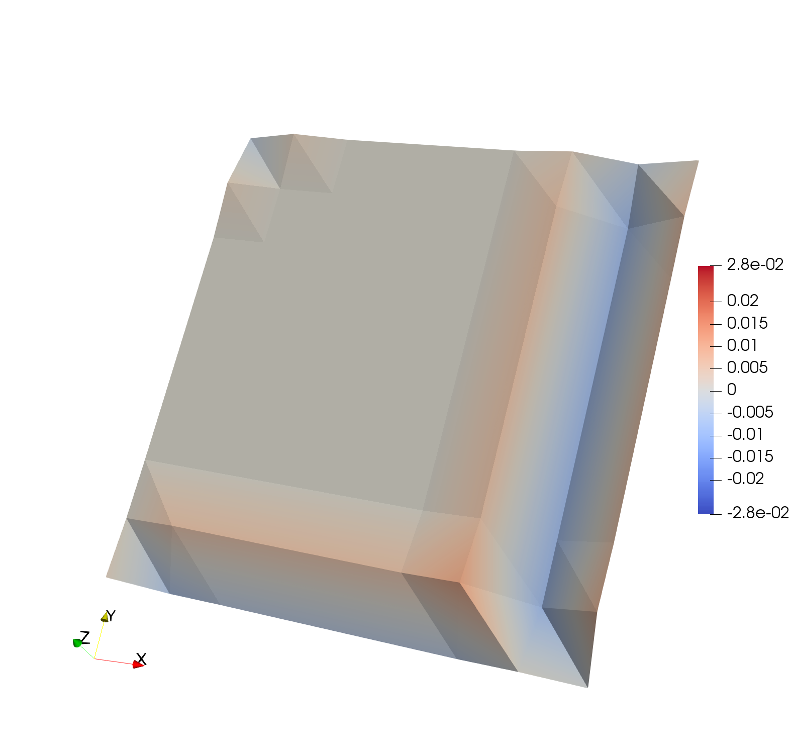
(a) $G_{T}({\mathbf{u}}_{c,\;T},\;{\mathbf{g}}_{c,\;T})$

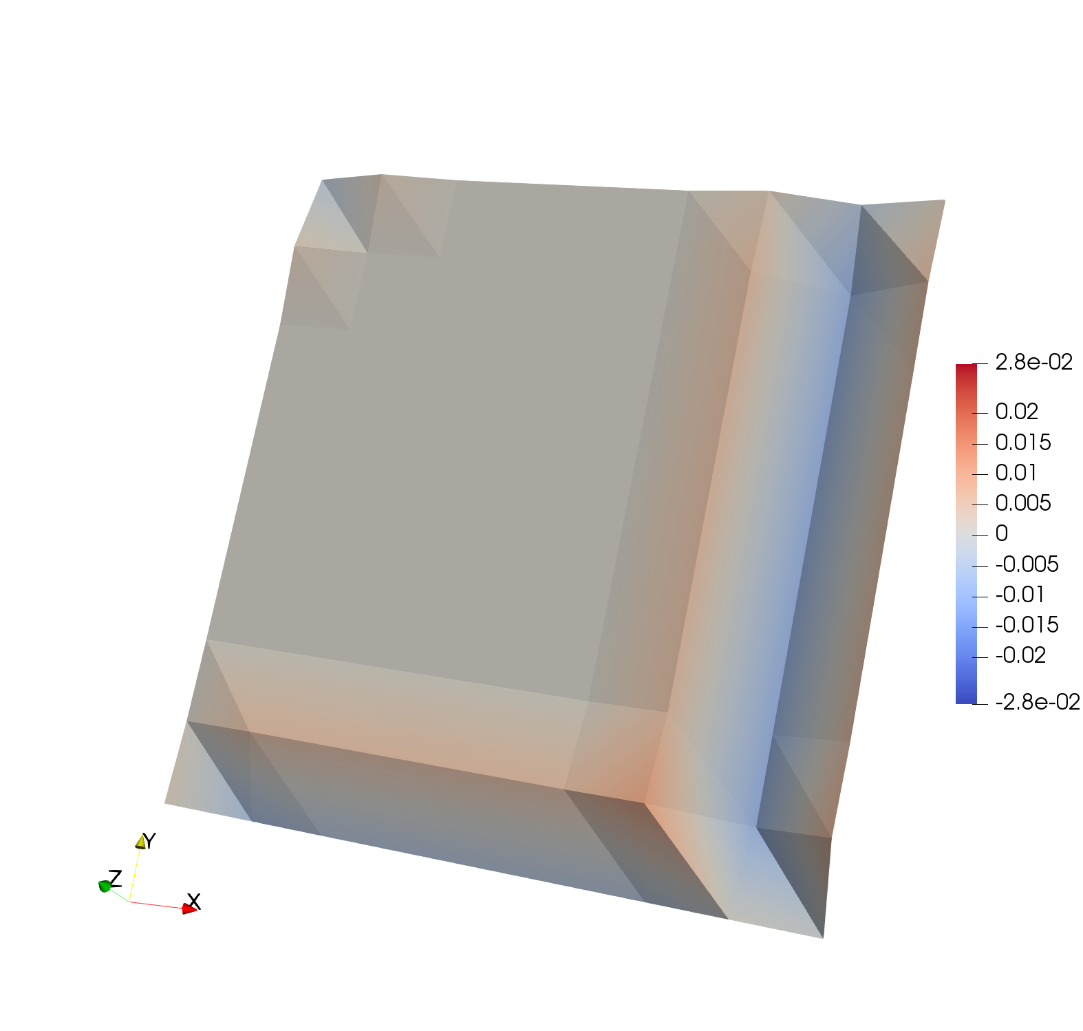
(b) $G_{T_{DNN}}({\mathbf{u}}_{c,\;T},\;{\mathbf{g}}_{c,\;T})$

Figure 5. Plots of $G_{T}$ and $G_{T_{DNN}}$ for sixty four subdomains at the $({\mathbf{u}}_{c,\;T},\;{\mathbf{g}}_{c,\;T})$ which achieves the min $L_{2}$ error. The min relative error is $1.493536E{-07}$.

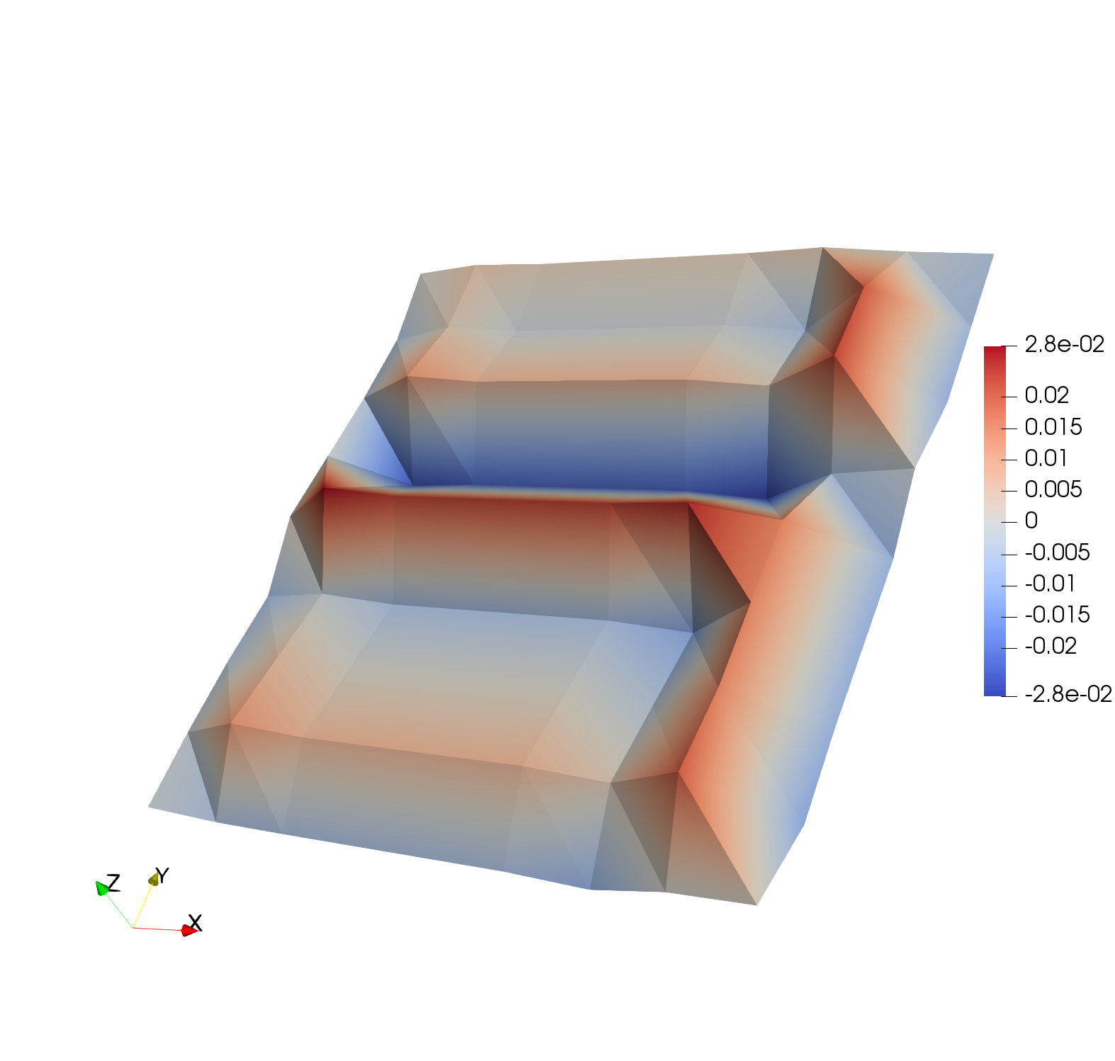
(a) $G_{T}({\mathbf{u}}_{c,\;T},\;{\mathbf{g}}_{c,\;T})$

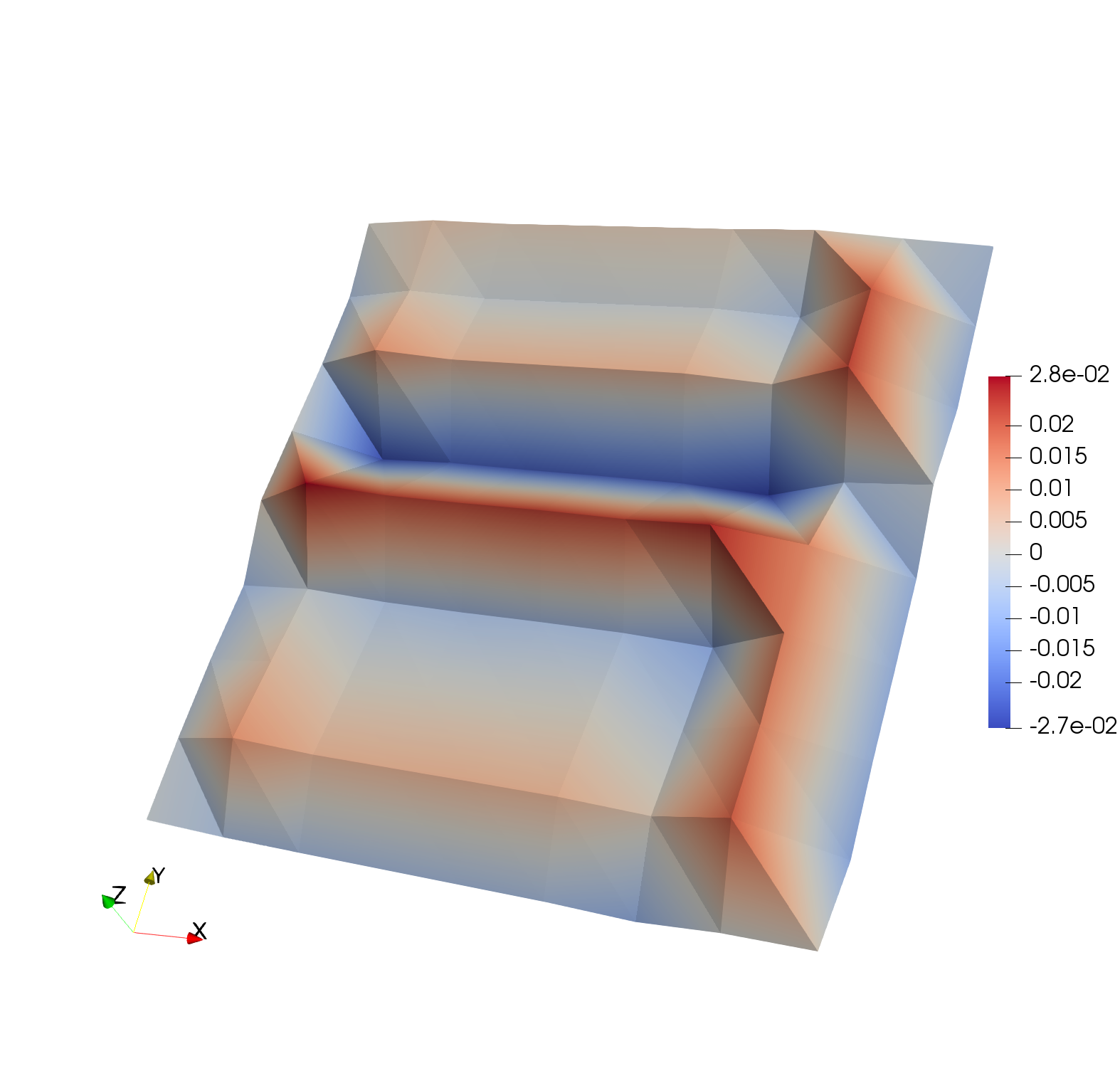
(b) $G_{T_{DNN}}({\mathbf{u}}_{c,\;T},\;{\mathbf{g}}_{c,\;T})$

Figure 6. Plots of $G_{T}$ and $G_{T_{DNN}}$ for sixty four subdomains at the $({\mathbf{u}}_{c,\;T},\;{\mathbf{g}}_{c,\;T})$ which achieves the max $L_{2}$ error. The max relative error is $2.717447E{-05}$.

3. Application of DNN approximate coarse mappings in two-level FAS

3.1. The FAS algorithm

A standard approach for solving (2.1) is to use Newton’s method. The latter is an iterative process in which given a current iterate ${\mathbf{u}}$, we compute the next one, ${\mathbf{u}}_{next}$, by solving the Jacobian equation

(3.1) $$J_{F}({\mathbf{u}}){\mathbf{y}}={\mathbf{r}}:={\mathbf{f}}-F({\mathbf{u}}),$$

and then ${\mathbf{u}}_{next}={\mathbf{u}}+{\mathbf{y}}$.

Typically, the Jacobian problem (3.1) is solved by an iterative method such as GMRES (generalized minimal residual).

To speed-up the convergence, for nonlinear equations coming from finite element discretizations of elliptic PDEs, such as (2.2), we can exploit hierarchy of discretizations. A popular method is the two-level FAS (full approximation scheme) proposed by Achi Brandt, ([2]) (see also ([20])). For a recent convergence analysis of FAS, we refer to ([3]).

To define the two-level FAS, we need a coarse version of $F$, which is another nonlinear mapping $F_{c}:\;{\mathbb{R}}^{n_{c}}\mapsto{\mathbb{R}}^{n_{c}}$, for some $n_{c}<n$. We also need its Jacobian $J_{c}=J_{F_{c}}$. Again, we assume that both are available via their actions (by calling some appropriate functions). To communicate data between the original, fine level, ${\mathbb{R}}^{n}$ and the coarse level, ${\mathbb{R}}^{n_{c}}$, we are given two linear mappings (matrices):

• Coarse-to-fine (interpolation or prolongation) mapping $P:\;{\mathbb{R}}^{n_{c}}\mapsto{\mathbb{R}}^{n}$.

• Fine-to-coarse projection $\pi:\;{\mathbb{R}}^{n}\mapsto{\mathbb{R}}^{n_{c}}$, more precisely, we assume that $\pi P=I$ (then $(P\pi)^{2}=P\pi$ is a projection). In our finite element setting, $\pi$ is simply the restriction of a fine-grid vector ${\mathbf{u}}$ to the coarse dofs, i.e., $\pi=[0,\;I]$, where the columns in $I$ correspond to the coarse dofs viewed as subset of the the fine dofs.

Then, the two-level FAS (TL-FAS) can be formulated as follows.

Algorithm 3.1 (Two-level FAS).

For problem (2.1), with a current approximation ${\mathbf{u}}$, the two-level FAS method performs the following steps to compute the next approximation ${\mathbf{u}}_{next}$.

• For a given $m\geq 1$ apply $m$ steps of (inexact) Newton algorithm, (3.1), to compute ${\mathbf{y}}_{m}$ and let ${\mathbf{u}}_{\frac{1}{3}}={\mathbf{u}}+{\mathbf{y}}_{m}$.

• Form the coarse-level nonlinear problem for ${\mathbf{u}}_{c}$

  (3.2) $$F_{c}({\mathbf{u}}_{c})={\mathbf{f}}_{c}\equiv F_{c}(\pi{\mathbf{u}}_{\frac{1}{3}})+P^{T}({\mathbf{f}}-F({\mathbf{u}}_{\frac{1}{3}})).$$

• Solve (3.2) accurately enough using Newton’s method based on the coarse Jacobian $J_{c}$ and initial iterate ${\mathbf{u}}_{c}:=\pi{\mathbf{u}}_{\frac{1}{3}}$. Here we use enough iterations of GMRES for solving the resulting coarse Jacobian residual equations

  $$J_{c}({\mathbf{u}}_{c}){\mathbf{y}}_{c}={\mathbf{r}}_{c}={\mathbf{f}}_{c}-F_{c}({\mathbf{u}}_{c}),\text{ and let }{\mathbf{u}}_{c}:={\mathbf{u}}_{c}+{\mathbf{y}}_{c},$$

  until a desired accuracy is reached.

• Update fine-level approximation

  $${\mathbf{u}}_{\frac{2}{3}}={\mathbf{u}}_{\frac{1}{3}}+P({\mathbf{u}}_{c}-\pi{\mathbf{u}}_{\frac{1}{3}}).$$

• Repeat the FAS cycle starting with ${\mathbf{u}}:={\mathbf{u}}_{next}={\mathbf{u}}_{\frac{2}{3}}$ until a desired accuracy is reached.

In what follows, we use the following equivalent form of the TL-FAS. At the coarse level, we will represent ${\mathbf{u}}_{c}:={\mathbf{u}}^{0}_{c}+{\mathbf{g}}_{c}$, where ${\mathbf{u}}^{0}_{c}=\pi{\mathbf{u}}_{\frac{1}{3}}$ is the initial coarse iterate coming from the fine level, and we will be solving for the correction ${\mathbf{g}}_{c}$. That is, the coarse problem in terms of the correction reads

$${\overline{F}}_{c}({\mathbf{g}}_{c})={\overline{\mathbf{f}}}_{c},$$

where

$$\begin{array}[]{rl}{\overline{F}}_{c}({\mathbf{g}}_{c})&\equiv G_{c}({\mathbf{u}}^{0}_{c},\;{\mathbf{g}}_{c})=F_{c}({\mathbf{u}}^{0}_{c}+{\mathbf{g}}_{c})-F_{c}({\mathbf{u}}^{0}_{c})\\ {\overline{\mathbf{f}}}_{c}&\equiv P^{T}({\mathbf{f}}-F({\mathbf{u}}_{\frac{1}{3}}))={\mathbf{f}}_{c}-F_{c}({\mathbf{u}}^{0}_{c}).\end{array}$$

The rest of the algorithm does not change, in particular, we have

$$\begin{array}[]{rl}{\mathbf{r}}_{c}&={\mathbf{f}}_{c}-F_{c}({\mathbf{u}}_{c})\\ &={\mathbf{f}}_{c}-F_{c}({\mathbf{u}}^{0}_{c}+{\mathbf{g}}_{c})\\ &={\overline{\mathbf{f}}}_{c}+F_{c}({\mathbf{u}}^{0}_{c})-F_{c}({\mathbf{u}}^{0}_{c}+{\mathbf{g}}_{c})\\ &={\overline{\mathbf{f}}}_{c}-G_{c}({\mathbf{u}}^{0}_{c},\;{\mathbf{g}}_{c})\\ &={\overline{\mathbf{f}}}_{c}-{\overline{F}}_{c}({\mathbf{g}}_{c}),\end{array}$$

and

$${\mathbf{u}}_{\frac{2}{3}}={\mathbf{u}}_{\frac{1}{3}}+P({\mathbf{u}}_{c}-\pi{\mathbf{u}}_{\frac{1}{3}})={\mathbf{u}}_{\frac{1}{3}}+P({\mathbf{u}}_{c}-{\mathbf{u}}^{0}_{c})={\mathbf{u}}_{\frac{1}{3}}+P{\mathbf{g}}_{c}.$$

3.1.1. The choice for $F_{c}$ using DNN

In our finite element setting, a true (Galerkin) coarse operator is $P^{T}F(P(.))$, where $P$ is the piecewise linear interpolation mapping and $F$ is the fine level nonlinear finite element operator. We train the global coarse actions based on the fact that the actions of $F$ and $P$ can be computed subdomain-by-subdomain employing standard finite element assembly procedure, as described in the previous section. That is, $F$ can be assembed by local $F_{T}$s and the coarse $P^{T}F(P(.))$ can be assembled from local coarse actions $P^{T}_{T}F_{T}(P_{T}(.))$ based on local versions $\{P_{T}\}$ of $P$.

More specifically, we train for each subdomain $T\in{\mathcal{T}}_{H}$ a DNN which takes as input any pair of coarse vectors ${\mathbf{v}}_{c,T},\;{\mathbf{g}}_{c,\;T}\in{\mathbb{R}}^{n_{c}}$ and produces $P^{T}_{T}F_{T}(P_{T}({\mathbf{v}}_{c,T}+{\mathbf{g}}_{c,T}))-P^{T}_{T}F_{T}(P_{T}{\mathbf{v}}_{c,T})\in{\mathbb{R}}^{n_{c}}$ as our desired output. The global action $P^{T}F(P({\mathbf{v}}_{c}+{\mathbf{g}}_{c}))-P^{T}F(P({\mathbf{v}}_{c}))$ is computed by assembling all local actions, and we use the same assembling procdeure for the approximations obtained using the trained local DNNs.

The trained this way DNN gives the actions of our coarse nonlinear mapping ${\overline{F}}_{c}(.)$.

3.2. Some details on implementing TL-FAS algorithm

We are solving the nonlinear equation $F({\mathbf{u}})={\mathbf{f}}$ where the actions of $F:\;{\mathbb{R}}^{n}\mapsto{\mathbb{R}}^{n}$ are available. Also, we assume that we can compute its Jacobian matrix for any given ${\mathbf{u}}$, $J({\mathbf{u}})$.

We are also given an interpolation matrix $P:\;{\mathbb{R}}^{n_{c}}\mapsto{\mathbb{R}}^{n}$. Finally, we have a mapping $\pi:\;{\mathbb{R}}^{n}\mapsto{\mathbb{R}}^{n_{c}}$ such that $\pi P=I$ on ${\mathbb{R}}^{n_{c}}$. This implies that $P\pi$ is a projection, i.e, $(P\pi)^{2}=P\pi$.

Consider the coarse nonlinear mapping $F({\mathbf{u}}_{c})\equiv P^{T}(F(P{\mathbf{u}}_{c})):\;{\mathbb{R}}^{n_{c}}\mapsto{\mathbb{R}}^{n_{c}}$.

We assume that an approximation $G({\mathbf{v}}_{c},\;{\mathbf{g}}_{c})$ to the mapping

$$F_{c}({\mathbf{v}}_{c}+{\mathbf{g}}_{c})-F_{c}({\mathbf{v}}_{c}),$$

is available through its actions for a set of input vectors ${\mathbf{v}}_{c}$ varying in a given box $K$ and for another input vector ${\mathbf{g}}_{c}$ varying in a small ball $B$ about the origin. For a fixed ${\mathbf{v}}_{c}$, we denote ${\overline{F}}_{c}({\mathbf{g}}_{c})=G({\mathbf{v}}_{c},\;{\mathbf{g}}_{c})$.

We are interested in the following two-level FAS algorithm for solving $F({\mathbf{u}})={\mathbf{f}}$.

Algorithm 3.2 (TL-FAS).

Input parameters:

• Initial approximation ${\mathbf{u}}_{0}$ sufficiently close to the exact solution ${\mathbf{u}}_{*}$. For a problem with a known solution, we choose ${\mathbf{u}}_{0}={\mathbf{u}}_{*}+\tau\times(\text{random vector})$, where $\tau$ is an input (e.g., $\tau=1,\;0.1,\;10.0,...$). The random vector has as components random numbers in $(-1,1)$.

• $\delta$ (e.g., $\delta=0.1$, or $\delta=0.5$) - tolerance used in GMRES to solve approximately the fine-level Jacobian equations.

• Maximal number $N_{\max}=1,2\text{ or }4,$ of fine-level inexact Newton iterations

• Additionally, maximal number of GMRES iterations, $I_{\max}=2,\text{ or }5,$ allowed in solving the fine-level Jacobian equations.

• $\delta_{c}$ (e.g., $\delta_{c}=10^{-3}$), tolerance used in GMRES for solving coarse-level Jacobian equations.

• $\tau_{c}$ (equal to $1$ or $0.1$, or $0.01$) - step length in coarse-level inexact Newton iterations.

• Maximal number of coarse-level GMRES iterations, $I^{c}_{\max}=1000$.

• Maximal number of inexact coarse-level Newton iterations , $N^{c}_{\max}=10\text{ or }100$.

• Maximal number of FAS iterations, $N_{FAS}=10$.

• Tolerance for FAS iterations, $\epsilon=10^{-6}$.

With the above input specified, a TL-FAS algorithm takes the form:

• FAS-loop: If visited $<N_{FAS}$ times perform the steps below. Otherwise exit.

  • Perform $N_{\max}$ fine-level inexact Newton iterations, which involve the following steps:

    • For the current iterate ${\mathbf{u}}$ (the initial one, ${\mathbf{u}}={\mathbf{u}}_{0}$, is given as input) compute residual

      $${\mathbf{r}}={\mathbf{f}}-F({\mathbf{u}}).$$

    • Compute Jacobian $J({\mathbf{u}})$.

    • Solve approximately the Jacobian equation

      $$J({\mathbf{u}}){\mathbf{y}}={\mathbf{r}},$$

      using at most $I_{\max}$ GMRES iterations or until reaching tolerance $\delta$, i.e.,

      $$\|J({\mathbf{u}}){\mathbf{y}}-{\mathbf{r}}\|\leq\delta\;\|{\mathbf{r}}\|.$$

    • Update ${\mathbf{u}}:={\mathbf{u}}+{\mathbf{y}}$.

  • Compute fine-level Jacobian $J({\mathbf{u}})$ and the coarse-level one $J_{c}=P^{T}J({\mathbf{u}})P$.

  • Compute ${\mathbf{u}}_{c}=\pi{\mathbf{u}}$.

  • Coarse-loop for solving

    $${\overline{\mathbf{F}}}_{c}({\mathbf{g}}_{c}):=G({\mathbf{u}}_{c},{\mathbf{g}}_{c})={\overline{\mathbf{f}}}_{c}\equiv P^{T}({\mathbf{f}}-F({\mathbf{u}})),$$

    with initial guess ${\mathbf{g}}_{c}=0$ where we keep ${\mathbf{u}}_{c}$ and the coarse Jacobian $J_{c}$ fixed. The coarse-level loop reads:

    • Compute coarse residual

      $${\mathbf{r}}_{c}={\overline{\mathbf{f}}}_{c}-{\overline{F}}_{c}({\mathbf{g}}_{c}).$$

    • Solve by GMRES, $J_{c}{\mathbf{y}}_{c}={\mathbf{r}}_{c}$ using at most $I^{c}_{\max}$ iterations or until we reach $\|J_{c}{\mathbf{y}}_{c}-{\mathbf{r}}_{c}\|\leq\delta_{c}\;\|{\mathbf{r}}_{c}\|.$

    • Update

      $${\mathbf{g}}_{c}:={\mathbf{g}}_{c}+\tau_{c}{\mathbf{y}}_{c}.$$

    • Repeat at most $N^{c}_{\max}$ times the above three steps of the coarse-level loop.

  • Update fine-level iterate

    $${\mathbf{u}}:={\mathbf{u}}+P{\mathbf{g}}_{c}.$$

  • If $\|F({\mathbf{u}})-{\mathbf{f}}\|>\epsilon\|F({\mathbf{u}}_{0})-{\mathbf{f}})\|$, go to the beginning of FAS-loop. Otherwise exit.

3.3. Local tools for FAS

We stress again that all global actions of the coarse operator (exact and approimate via DNNs) are realized by assembly of local actions. All this is possible due to the inherent nature of the finite element method. We illustrate the local subdomains in Fig. 7 and Fig. 8.

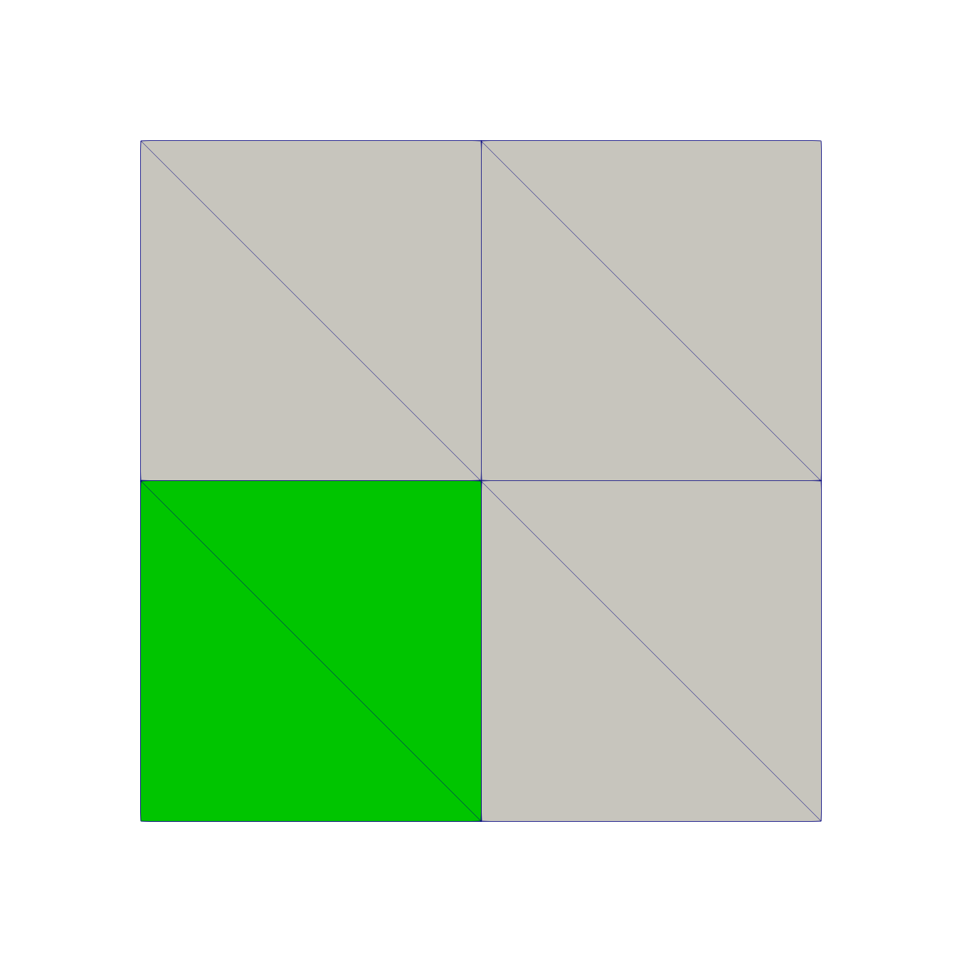
(a) Global coarse mesh

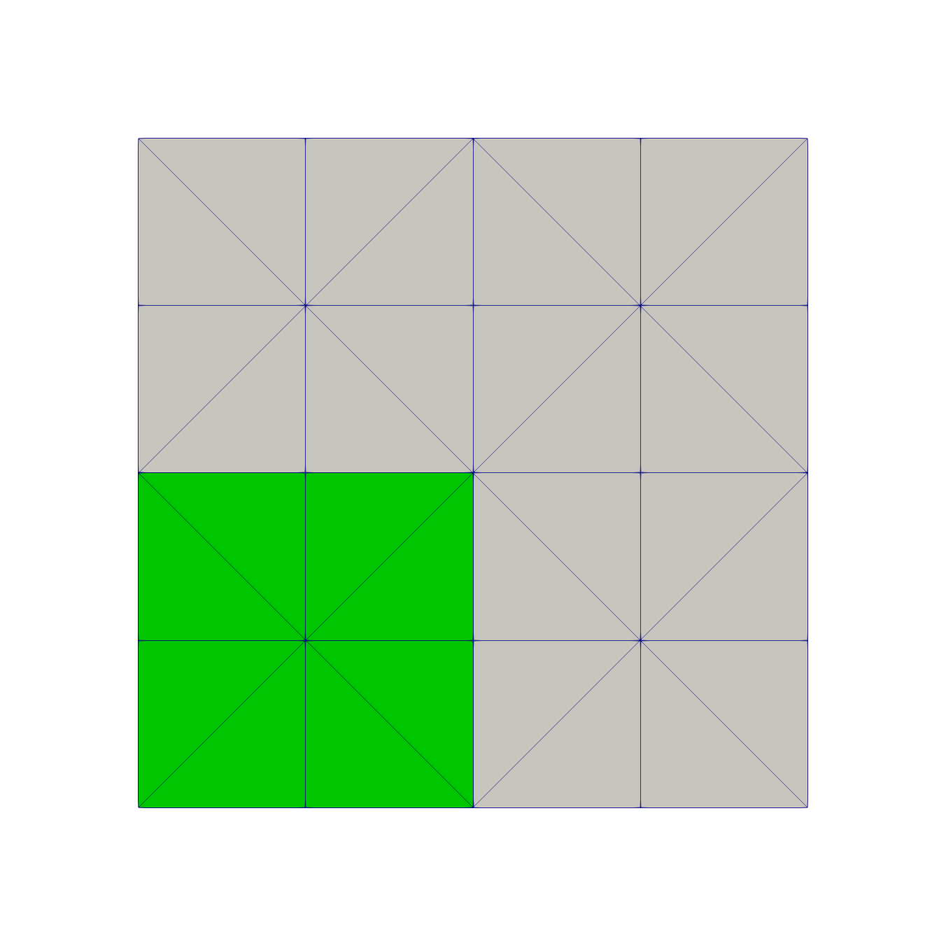
(b) Global fine mesh

Figure 7. An example of domain decomposition for 4 subdomains when we have $H/h=2$.

(a) Global coarse mesh

(b) Global fine mesh

Figure 8. A visualization when we have 4 subdomains and $H/h=4$.

More specifically, in Figures 7 and 8 , on the left we have an example of a global coarse mesh ${\mathcal{T}}_{H}$, with the shaded area being the submesh contained in $T\in\Omega_{H}$ -one of the four subdomains in ${\mathcal{T}}_{H}$. On the right, we show the submesh of the global fine mesh ${\mathcal{T}}_{h}$ restricted to the subdomain $T$.

3.4. Some details on implementing TL-FAS with DNNs

Using the tools and algorithms from the previous sections, we first outline an implementation that involves training inside FAS and then present the algorithm for training outside the FAS. Training on the outside is useful because the training is then only part of a one time set up cost and independent of the r.h.s. The two-level training inside FAS is formulated as follows.

Algorithm 3.3 (Training inside FAS).

With the inputs specified in algorithm 3.2, the training inside takes the following steps

• Perform $N_{\max}$ fine-level inexact Newton iterations, which involve steps in algorithm 3.2 and update ${\mathbf{u}}$.

• Compute fine-level Jacobian $J({\mathbf{u}})$ and the coarse-level one $J_{c}=P^{T}J({\mathbf{u}})P$.

• Compute ${\mathbf{u}}_{c}=\pi{\mathbf{u}}$.

• We generate samples which are in the neighborhood of ${\mathbf{u}}_{c}$. More specifically, we use a shifted box $K=\{{\mathbf{u}}_{c}\}+[-0.05,0.05]$ and draw $10$ to $20$ vectors ${\mathbf{u}}_{c}$ from $K$ and $30$ to $50$ vectors ${\mathbf{g}}_{c}$ from the ball $B$ with radius $\delta_{B}=0.005$. We use these sets as inputs for training the DNNs to get the approximations of $G_{c,\;T}$ for each subdomain $T\in{\mathcal{T}}_{H}$ and assemble them into a global coarse action, $G_{c}$. Next, we enter the coarse-level loop as in Algorithm 3.2 and the rest of the algorithm remains the same. Note that the training is done only for the first fine-level iterate ${\mathbf{u}}$.

The following implementation gives the approximations of $G_{c,\;T}$ for each subdomain $T$ and can be performed outside the Algorithm 3.2.

Algorithm 3.4 (Training outside FAS).

Given the inputs specified in algorithm 3.2,in order to get the approximations of $G_{c,\;T}$ we proceed the training outside as follows

• We take $M$ inputs ${\mathbf{u}}$ from the box $K=[-0.05,0.05]$, and $m$ corrections ${\mathbf{g}}$ are drawn from the ball $B$ of radius $\delta_{B}=0.005$. This gives a training set with $M\times n$ vectors.

• We then use these vectors as inputs and train the neural networks which provide approximations of $G_{c,\;T}$ for each subdomain $T\in{\mathcal{T}}_{H}$. The latter after assembly give the global coarse action, $G_{c}$.

• Next, we enter Algorithm 3.2 with this approximate $G_{c}$ and the rest of the algorithm remains the same.

3.5. Comparative results for FAS with exact and approximate coarse operators using DNNs

In this section, we present some results for two level FAS using the exact operators and its approximation from the training inside and outside as mentioned in the previous section.

We perform the tests with the neural networks using the same settings in section 2.3 and test our algorithm for problem 2.1 with exact solution is $u_{*}=x^{2}(1-x)^{2}+y^{2}(1-y)^{2}$ on the unit square in $\mathbb{R}^{2}$ with $H/h=2$. For the FAS algorithm, we use the following parameters:

• Initial approximation ${\mathbf{u}}_{0}={\mathbf{u}}_{*}+\tau\times(\text{random vector})$, where $\tau=2$ and the random vector has as components random numbers in $(-1,1)$.

• $\delta=10^{-6}$ - tolerance used in GMRES to approximately solve the fine-level Jacobian equations.

• Maximal number $N_{\max}=2$ of fine-level inexact Newton iterations and tolerance is $0.01$.

• Maximal number of GMRES iterations, $I_{\max}=4$ allowed in solving the fine-level Jacobian equations.

• $\delta_{c}=10^{-8}$, tolerance used in GMRES for solving coarse-level Jacobian equations.

• $\tau_{c}=0.1$ - step length in coarse-level inexact Newton iterations for FAS two levels with true operators, FAS training inside, and $\tau_{c}=0.0001$ for FAS training outside.

• Maximal number of coarse-level GMRES iterations, $I^{c}_{\max}=10$.

• Maximal number of inexact coarse-level Newton iterations , $N^{c}_{\max}=5$ with tolerance $10^{-4}$.

• Maximal number of FAS iterations, $N_{FAS}=10$.

• Tolerance for FAS iterations, $\epsilon=10^{-6}$.

We present the results in Table 3.5 (TL-FAS with true coarse operator), Table 3.5 (TL-FAS with training inside), and Table 3.5 (TL-FAS with training outside). It can be seen that the training inside does give similar results to the true operators and even better in terms of relative residuals. For four subdomains, the training outside reached the same number of iterations in FAS as in Tables 3.5 and 3.5. However, we did not achieve as small residuals as we could in the previous two cases. When we have more subdomains, the training outside requires more iterations on the coarse level than the other two approaches, but nevertheless it still meets the desired tolerance.

# of subdomains	True Operators
	FAS iteration	# coarse iterations	Relative residuals
4	1	5	0.174041
	2	5	0.003939
	3	5	4.377789E-06
	4	1	1.081675E-11
16	1	5	0.161382
	2	5	0.001406
	3	1	3.843124E-07
64	1	5	0.162089
	2	5	0.002728
	3	1	2.393705E-06
	4	1	1.141114E-09

tableResults for FAS using true operators with different number of subdomains using $k=1+u^{2}$.

# of subdomains	Approximate Operators with inside training
	FAS iteration	# coarse iterations	Relative residuals
4	1	5	0.171590
	2	5	0.003733
	3	1	3.826213E-06
	4	1	8.325530e-12
16	1	5	0.160120
	2	5	0.001286
	3	1	2.946412E-07
64	1	5	0.159982
	2	5	0.001521
	3	1	4.671780E-07

tableResults for training NNs inside with different number of subdomains using $k=1+u^{2}$.

# of subdomains	Approximate Operators with outside training
	FAS iteration	# coarse iterations	Relative residuals
4	1	5	0.186189
	2	5	0.004746
	3	5	5.300791E-06
	4	5	5.623933e-10
16	1	5	0.174228
	2	5	0.002257
	3	5	1.246687E-06
	4	5	4.025110E-09
64	1	5	0.176886
	2	5	0.004503
	3	5	1.488866E-05
	4	5	2.061581E-08

tableResults for training NNs outside with different number of subdomains using $k=1+u^{2}$.

We also studied the case $H/h=4$ with the same setting as above for the neural networks, the same $k=1+u^{2}$ and the exact solution. The following tables (Tables 3.5, 3.5, and 3.5) represent the results for 4 and 16 subdomains. They show similar behaviour as in the previous case of $H/h=2$.

# of subdomains	True Operators
	FAS iteration	# coarse iterations	Relative residuals
4	1	5	0.171241
	2	5	0.002991
	3	1	2.325478E-06
	4	1	6.696561e-12
16	1	5	0.168299
	2	5	0.002804
	3	1	4.457398E-06
	4	1	3.394781E-08

tableResults for FAS using true operators with $H/h=4$.

# of subdomains	Approximate Operators with inside training
	FAS iteration	# coarse iterations	Relative residuals
4	1	5	0.172198
	2	5	0.003446
	3	1	1.292521E-06
	4	1	6.055108e-12
16	1	5	0.167623
	2	5	0.002594
	3	5	4.748181E-06
	4	1	2.390020E-09

tableResults for NNs training inside with $H/h=4$.

# of subdomains	Approximate Operators with outside training
	FAS iteration	# coarse iterations	Relative residuals
4	1	5	0.172328
	2	5	0.003307
	3	1	3.165177E-06
	4	1	2.408886e-10
16	1	5	0.168451
	2	5	0.002085
	3	5	1.009380E-06
	4	1	2.813398E-09

tableResults for NNs training outside with $H/h=4$.

3.5.1. Cost of training

To get a sense of the cost, for the case of 4 subdomains and $H/h=2$, we display the accuracy and the loss values, characteristics provided by Keras, commonly used in training DNNs. Here, we only present the results for one of the four subdomains since the outcomes are similar for all other subdomains. Figure 9 shows plots for training inside whereas Figure 10 for the training outside FAS.

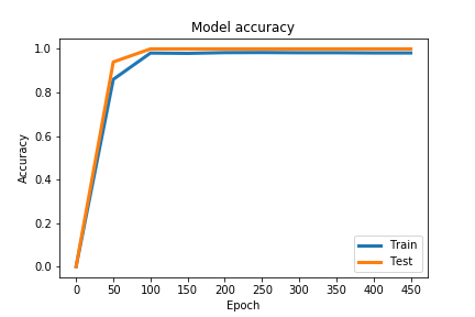
(a) Training and testing accuracy

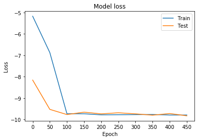
(b) Training and testing loss

Figure 9. Plots of the accuracy at every 50 epochs and the log scale of loss values at every 50 epochs for one subdomain. We use $80\%$ of the number of vectors for training purpose and $20\%$ for testing. Here, we do the training inside the FAS.

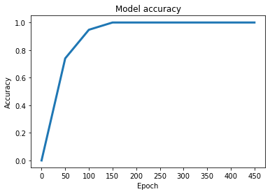
(a) Training and testing accuracy

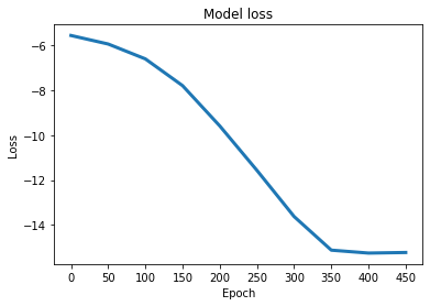
(b) Training and testing loss

Figure 10. We do the training outside the FAS and use all the data/vectors for testing the accuracy as well as the loss values. We plot the accuracy at every 50 epochs and the log scale of loss values at every 50 epochs for one subdomain.

3.5.2. Results for different nonlinear coefficients $k=k(u)$

Next, we consider 4 subdomains with $H/h=2$ for different coefficients $k$. We use the same settings for the initial inputs and the neural networks as specified at the beginning of this section. We see in Table 3.5.2, Table 3.5.2, Table 3.5.2, Table 3.5.2, Table 3.5.2 and Table 3.5.2 that the results are comparable for all of the used coefficients $k=k(u)$.

More specifically, the results for $k=1+e^{-u}+x^{2}+y^{2}$ are found in Table 3.5.2, Table 3.5.2, Table 3.5.2.

FAS iteration	# coarse iterations	Relative residuals
1	5	0.128534
2	5	0.000738
3	1	3.857236E-07

tableResults for FAS using true operators

FAS iteration	# coarse iterations	Relative residuals
1	5	0.127007
2	5	0.000706
3	1	2.677881E-07

tableResults for FAS with training inside

FAS iteration	# coarse iterations	Relative residuals
1	5	0.141989
2	5	0.001091
3	5	7.363723E-07

tableResults for FAS with training outside

Similarly, for $k=1+e^{-u}$, we have the results displayed in Table 3.5.2, Table 3.5.2 and Table 3.5.2.

FAS iteration	# coarse iterations	Relative residuals
1	5	0.127675
2	5	0.000701
3	1	2.662172E-07

tableResults for FAS with true operators

FAS iteration	# coarse iterations	Relative residuals
1	5	0.124039
2	5	0.000535
3	1	1.782604E-07

tableResults for FAS with training inside

FAS iteration	# coarse iterations	Relative residuals
1	5	0.141077
2	5	0.001084
3	5	7.305067E-07

tableResults for FAS with training outside

3.5.3. Illustration of the computed approximate solutions

We also provide illustration for the approximate solutions obtained from Newton method using the nonlinear operators from the training outside FAS and project them back to the fine level along with the true solutions in the following figures 11, 12 and 13 for several subdomain cases. Here, we use the true solution $u=x^{2}(1-x)^{2}+y^{2}(1-y)^{2}$. These illustrations demonstrate the potential for using the trained DNNs as accurate discretization tool.

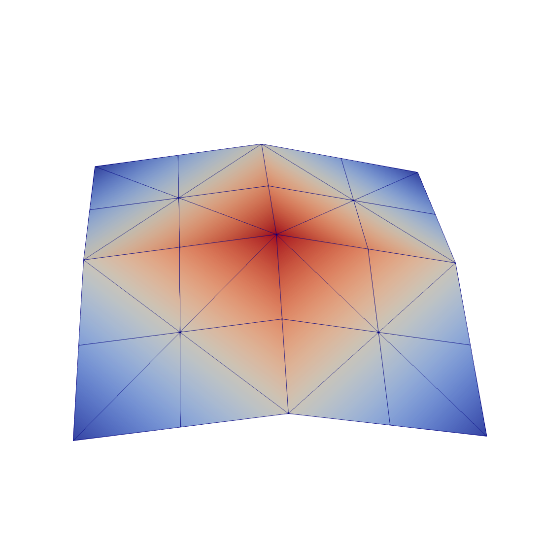
(a) True solution

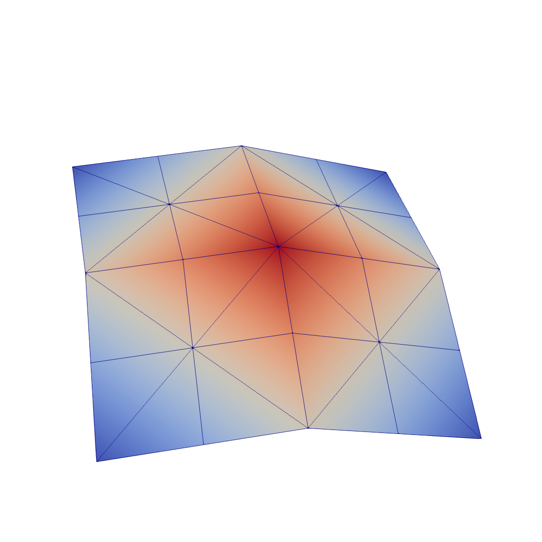
(b) Approximate solution

Figure 11. Plots of approximate and true solutions for 4 subdomains.

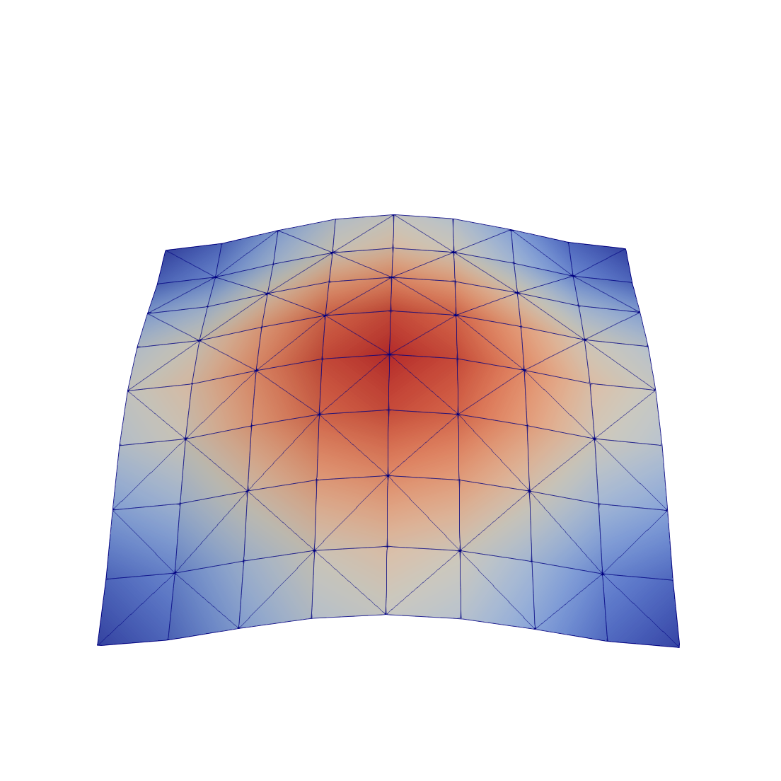
(a) True solution

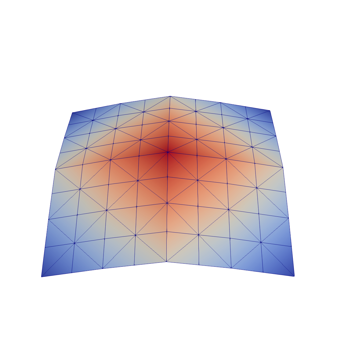
(b) Approximate solution

Figure 12. Plots of approximate and true solutions for 16 subdomains.

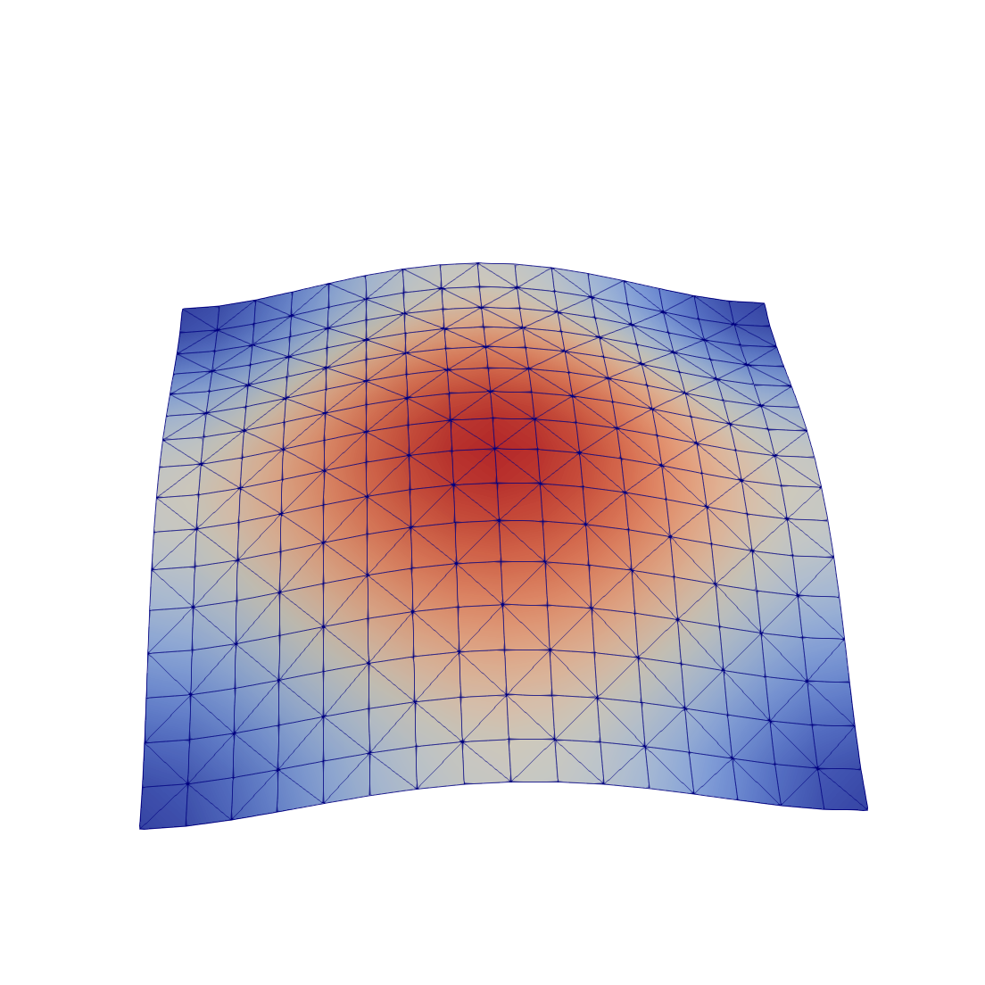
(a) True solution

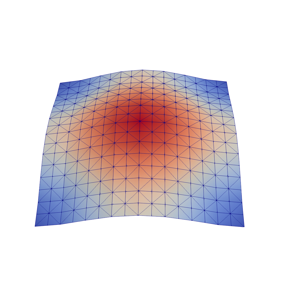
(b) Approximate solution

Figure 13. Plots of approximate and true solutions for 64 subdomains.

Similarly, we perform the test with the exact solution $u=\mbox{cos}(\pi x)\mbox{cos}(\pi y)$. Figure 14, 15, and 16 show the plots of approximate solutions and true solutions for different number of subdomains.

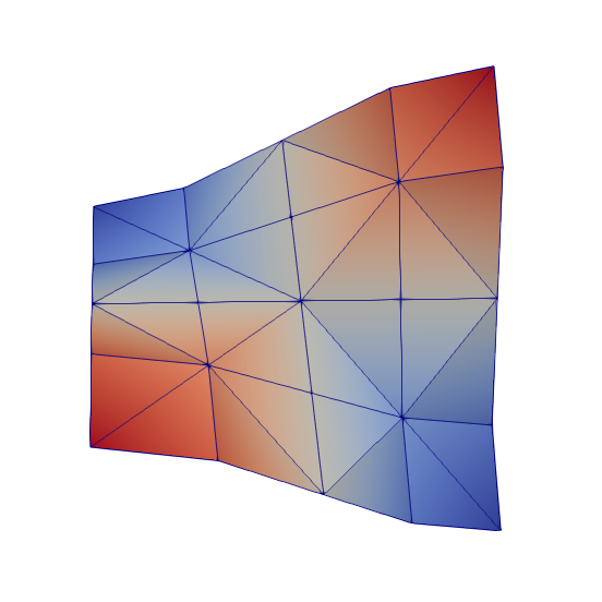
(a) True solution

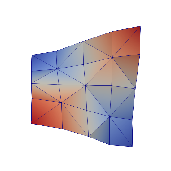
(b) Approximate solution

Figure 14. Plots of approximate and true solutions for 4 subdomains.

(a) True solution

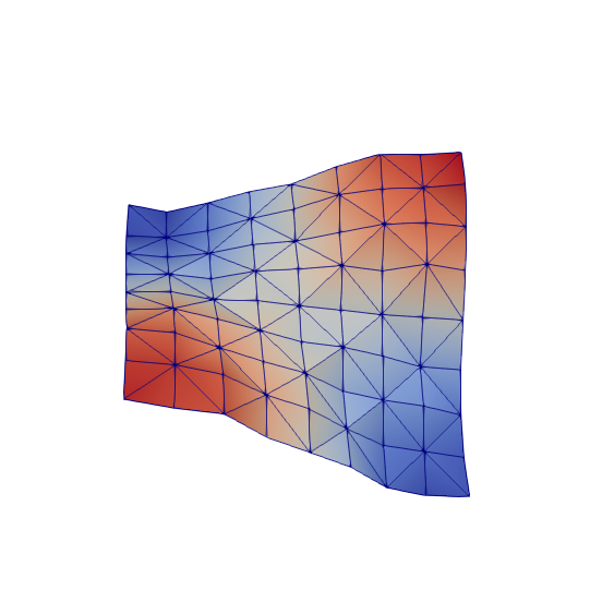
(b) Approximate solution

Figure 15. Plots of approximate and true solutions for 16 subdomains.

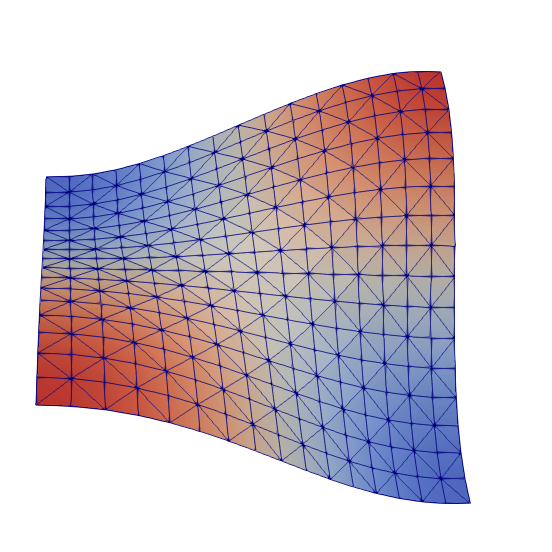
(a) True solution

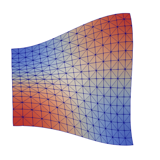
(b) Approximate solution

Figure 16. Plots of approximate and true solutions for 64 subdomains.

4. Conlusions and future work

The paper presented first encouraging results for approximating coarse finite element nonlinear operators for model diffusion reaction PDE in two dimensions. These operators were successfully employed in a two-level FAS for solving the resulting system of nonlinear algebraic equations. The resulting DNNs are quite expensive to replace the true Galerkin coarse nonlinear operators, however once constructed, one could in principle use them for solving the same type nonlinear PDEs with different r.h.s. Upto a certain extent we can control the DNN complexity by choosing larger ratio $H/h$ and finally, it is clear that the training since it is local, subdomain-by-subdomain, and independent of each other, one can exploit parallelism in the training. Another viable option is to use convolutional DNNs instead of the currently employed fully connected ones. Also, a natural next step is to apply recursion, thus ending up with a hierarchy of trained coarse DNNs for use as coarse nonlinear discretization operators. There is one more part where we can apply DNNs, namely to get approximations to the coarse Jacobians, $J_{c}({\mathbf{u}}_{c,T})$ (also done locally). Here, the input is the local coarse vector ${\mathbf{u}}_{c,\;T}$ and the output will be a local matrix $J_{c,T}({\mathbf{u}}_{c,T})$. It is also of interest to consider more general nonlinear, including stochastic, PDEs, which is a widely open area for future research.

Disclaimer

This document was prepared as an account of work sponsored by an agency of the United States government. Neither the United States government nor Lawrence Livermore National Security, LLC, nor any of their employees makes any warranty, expressed or implied, or assumes any legal liability or responsibility for the accu- racy, completeness, or usefulness of any information, apparatus, product, or pro- cess disclosed, or represents that its use would not infringe privately owned rights. Reference herein to any specific commercial product, process, or service by trade name, trademark, manufacturer, or otherwise does not necessarily constitute or im- ply its endorsement, recommendation, or favoring by the United States government or Lawrence Livermore National Security, LLC. The views and opinions of authors expressed herein do not necessarily state or reflect those of the United States gov- ernment or Lawrence Livermore National Security, LLC, and shall not be used for advertising or product endorsement purposes.

References

- [1] L. Bar and N. Sochen, Unsupervised deep learning algorithm for pde-based for- ward and inverse problems, 2019. arXiv: 1904.05417.
- [2] A. Brandt and O. Livne, Multigrid techniques, Society for Industrial and Applied Mathematics, 2011. DOI: 10.1137/1.9781611970753.
- [3] L. Chen, X. Hu, and S. M. Wise, Convergence analysis of a generalized full approximation storage scheme for convex optimization problems, submitted. 2018.
- [4] T. Chen and H. Chen, Universal approximation to nonlinear operators by neu- ral networks with arbitrary activation functions and its application to dynamical systems, Ieee transactions on neural networks, vol. 6, no. 4, pp. 911-917, 1995.
- [5] M. M. Chiaramonte and M. Kiener, Solving differential equations using neural networks, http://cs229.stanford.edu/proj2013/, 2017.
- [6] G. Cybenko, Approximation by superpositions of a sigmoidal function, Math- ematics of control, signals and systems, vol. 2, no. 4, pp. 303-314, Dec. 1989. [Online]. Available: https://doi.org/10.1007/BF02551274.
- [7] I. Daubechies, R. DeVore, S. Foucart, B. Hanin, and G. Petrova, Nonlinear approximation and (deep) relu networks, 2019. arXiv: 1905.02199.
- [8] I. Goodfellow, Y. Bengio, and A. Courville, Deep learning, The MIT Press, 2016.
- [9] J. Han, A. Jentzen, and W. E, Solving high-dimensional partial differential equations using deep learning, 2018. arXiv: 1707.02568.
- [10] J. He and J. Xu, Mgnet: A unified framework of multigrid and convolutional neural network, Science China Mathematics, vol. 62, no. 7, pp. 1331-1354, Jul. 2019. DOI: 10.1007/s11425-019-9547-2.
- [11] J.-T. Hsieh, S. Zhao, S. Eismann, L. Mirabella, and S. Ermon, Learning neural PDE Solvers with convergence guarantees, 2019. arXiv: 1906.01200.
- [12] T.-W. Ke, M. Maire, and S. X. Yu, Multigrid neural architectures, 2016. arXiv:1611.07661.
- [13] D. P. Kingma and J. Ba, Adam: A method for stochastic optimization, Corr, vol. abs/1412.6980, 2014.
- [14] S. Pal and S. Gulli, Deep learning with keras: Implementing deep learning models and neural networks with the power of python. Packt Publishing, 2017.
- [15] N. Shukla, Machine learning with tensorflow. Manning Publications Co., 2018.
- [16] J. W. Siegel and J. Xu, On the approximation properties of neural networks, 2019. arXiv:1904.02311.
- [17] I. M. Sobol’, On the distribution of points in a cube and the approximate eval- uation of integrals, USSR computational mathematics and mathematical physics, vol. 7, no. 4, pp. 86-112, 1967.
- [18] I. M. Sobol’, D. Asotsky, A. Kreinin, and S. Kucherenko, Construction and comparison of high-dimensional sobol’ generators, Wilmott, vol. 2011, no. 56, pp. 64-79, 2011.
- [19] G. Strang, Linear algebra and learning from data. Wellesley-Cambridge Press, Feb. 2019.
- [20] P. S. Vassilevski, Multilevel block factorization preconditioners: Matrix-basedanalysis and algorithms for solving finite element equations. Springer Science and Business Media, 2008.
- [21] D.-X. Zhou, Universality of deep convolutional neural networks, 2018. arXiv:1805.10769.