Benchmarking results for the Newton-Anderson method

Abstract

This paper primarily presents numerical results for the Anderson accelerated Newton method on a set of benchmark problems. The results demonstrate superlinear convergence to solutions of both degenerate and nondegenerate problems. The convergence for nondegenerate problems is also justified theoretically. For degenerate problems, those whose Jacobians are singular at a solution, the domain of convergence is studied. It is observed in that setting that Newton-Anderson has a domain of convergence similar to Newton, but it may be attracted to a different solution than Newton if the problems are slightly perturbed.

1 Introduction

The purpose of this paper is to present some standard benchmark tests, including both degenerate and nondegenerate problems, for Anderson acceleration applied to Newton iterations, referred to as the Newton-Anderson method. The motivation behind studying this method stems from the results of [1], where it was shown how Anderson acceleration can locally improve the convergence rate of linearly converging fixed-point iterations for nondegenerate problems, and from the numerical results of [2], where Anderson acceleration applied to Newton’s method was demonstrated to allow convergence for a finite element discretization of the steady Navier-Stokes equations with a Reynold’s number high enough to cause standard Newton iterations to diverge. In that setting, the convergence history for Newton-Anderson was similar to that of a damped Newton method.

A further investigation in [3] proved that in one dimension, Anderson($1$), Anderson acceleration with an algorithmic depth of $m=1$, applied to Newton provides higher order (superlinear) convergence to nonsimple roots of scalar equations. Newton alone is known to only provide linear convergence for such problems [4, Chapter 6], at the rate $1-1/p$, where $p$ is the multiplicity of the root. Generalizing to higher dimensions, it is reasonable to ask whether Newton-Anderson also provides superlinear convergence for degenerate systems: those whose Jacobians are singular at a solution. The convergence of Newton’s method for such systems has been shown to be locally linear, in the intersection of a ball and a star-shaped domain about the solution [5, 6]. The numerical results in subsection 2.2 indicate that Newton-Anderson can provide such locally superlinear convergence, and that an algorithmic depth of $m=1$ can be sufficient to accomplish this.

Results for the first accelerated Newton method of [7], which has been shown both theoretically and numerically to provide superlinear convergence for degenerate problems [7, 8, 9], are shown alongside Newton and Newton-Anderson. This method, which can be viewed either as a predictor-corrector or an extrapolation method applied to every other iteration, is similar in form to Anderson(1) (particularly when considered from the extrapolation viewpoint), but has convergence properties that are sensitive to the tuning of two parameters. This method will be referred to as accelerated-Newton (or KS-acc. N., in the tables of results). The advantage of Newton-Anderson(1), is that, to the present authors’ knowledge, there is not a robust method of determining a priori the two parameters, $C>0$ ($C\in\mathbb{R}$ as originally presented in [7]) and $\alpha\in(0,1)$, of the accelerated-Newton method. A brief discussion of convergence theory for Newton-Anderson in the nondegenerate setting is included in subsection 1.1. The analysis of the convergence properties of Newton-Anderson however, particularly in the degenerate setting, remains pending.

In Section 2, the Newton-Anderson method is first tested on problems from the standard benchmark problem set of [10] to identify further problem classes on which Newton-Anderson is either advantageous or disadvantageous; and, to identify problems or problem classes where Newton-Anderson($m$), with $m>1$, is preferable to Newton-Anderson(1). The only problem identified from this set that falls in the last category is the Powell badly scaled function. Another such example designed to demonstrate that there exist problems where depth $m>1$ is preferred is (D3.) shown in subsection 2.2. That degenerate problem was purposely designed to demonstrate Newton-Anderson($m$) converging at at iterate $x_{m+1}$, for a problem $f(x)=0$, of the form $f_{i}(x)=[(Ax-b)_{i}]^{p_{i}}$, where $f:\mathbb{R}^{n}\rightarrow\mathbb{R}^{n}$, and there are $m\leq n$ distinct exponents $p_{i}$.

Next, the iterative schemes tested on the problems of sections 2 and 3 are specified. Each one is given below in terms of a uniform damping parameter $\beta\in(0,1]$, as is standard practice for all but Algorithm 4. Damping ($\beta\neq 1$) was only used here for one problem, the Brown almost-linear function on $\mathbb{R}^{n}$, with $n=20$. In that case the damping factor $\beta=0.8$ improved the convergence of all methods tested.

Algorithm 1 (Newton’s method)

Set $\beta\in(0,1]$. Choose $x_{0}$.
For $k=0,1,\ldots$
Set $x_{k+1}=x_{k}-\beta[f^{\prime}(x_{k})]^{-1}f(x_{k})$

Algorithm 2 (Newton-Anderson(1) from [11])

Set $\beta\in(0,1]$. Choose $x_{0}$. Compute $w_{1}=-[f^{\prime}(x_{0})]^{-1}f(x_{0})$. Set $x_{1}=x_{0}+\beta w_{1}$
For $k=1,2,\ldots$
Compute $w_{k+1}=-[f^{\prime}(x_{k})]^{-1}f(x_{k})$
Compute $\gamma^{k+1}={(w_{k+1},w_{k+1}-w_{k})}/{\left\|{w_{k+1}-w_{k}}\right\|^{2}}$
Set $x_{k+1}=x_{k}+\beta w_{k+1}-\gamma^{k+1}\left((x_{k+1}-x_{k})+\beta(w_{k+1}-w_{k})\right)$

Algorithm 3 (Newton-Anderson($m$) from [11])

Set $\beta\in(0,1]$ and $m\geq 0$. Choose $x_{0}$. Compute $w_{1}=-[f^{\prime}(x_{0})]^{-1}f(x_{0})$. Set $x_{1}=x_{0}+\beta w_{1}$
For $k=1,2,\ldots$, set $m_{k}=\min\{k,m\}$
Compute $w_{k+1}=-[f^{\prime}(x_{k})]^{-1}f(x_{k})$
Set $F_{k}=\begin{pmatrix}(w_{k+1}-w_{k})&\ldots&(w_{k-m+2}-w_{k-m+1}\end{pmatrix}$, and $E_{k}=\begin{pmatrix}(x_{k}-x_{k-1})&\ldots&(x_{k-m+1}-x_{k-m})\end{pmatrix}$
Compute $\gamma^{k+1}=\operatorname{argmin}_{\gamma\in\mathbb{R}^{m}}\left\|{w_{k+1}-F_{k}\gamma}\right\|$
Set $x_{k+1}=x_{k}+\beta w_{k+1}-\left(E_{k}+\beta F_{k}\right)\gamma^{k+1}$

Algorithm 4 (Accelerated Newton from Theorem 1.3 of [7])

Set $\beta\in(0,1]$ and parameters $C>0$ and $\alpha\in(0,1)$. Choose $x_{0}$.
For $k=1,2,\ldots$
Compute $\hat{w}_{k+1}=-[f^{\prime}(x_{k})]^{-1}f(x_{k})$.
Set $y_{k+1}=x_{k}+\beta\hat{w}_{k+1}$
Compute $w_{k+1}=-[f^{\prime}(y_{k+1})]^{-1}f(y_{k+1})$
Set $x_{k+1}=y_{k+1}-(2-C\left\|{w_{k+1}}\right\|^{\alpha})w_{k+1}$

In accordance with [12], results are shown for Algorithm 4 with parameter choices $C=1$ and $\alpha=0.9$. In the cases where the iteration with those parameters failed to converge, results are additionally shown with parameters $C=0.35$ and $\alpha=0.1$. In [7], where Algorithm 4 is introduced, the given parameter range for $C$ is $\mathbb{R}$; however, $C>0$ appears to be standard in presented demonstrations of the method [7, 8, 9, 12], and $C\leq 0$ is not considered here.

If the norm $\|\cdot\|$ used in the optimization step of Algorithm 3 is induced by an inner product $(\,\cdot,\cdot\,)$, Algorithm 3 reduces to Algorithm 2, for $m=1$ (and reduces to Algorithm 1, for $m=0$). See [13, 14] for the equivalence of this form of the Anderson algorithm to that originally stated in [11], and [15] for a results on optimization in norms not induced by inner products. Throughout the remainder, the norm $\|\cdot\|$ will denote the $l_{2}$ norm over $\mathbb{R}^{n}$.

1.1 Convergence theory

Convergence and acceleration theory for Anderson acceleration applied to fixed-point iterations has been recently been studied under assumptions that the underlying fixed-point operator is contractive (linearly converging) [1, 2, 15, 16, 17], nonexpansive [18], or nondegenerate [1]. Here, a small contribution to the theoretical understanding of the method is introduced for the particular case of applying Anderson acceleration to Newton iterations. The first lemma shows for nondegenerate problems that Newton-Anderson($m$) displays superlinear convergence under the assumption that the optimization coefficients are bounded. The second lemma shows for Newton-Anderson(1) that if the direction cosine between consecutive update steps is bounded below unity (the update steps don’t become parallel), then the resulting optimization coefficient is bounded. This result is applied to the first lemma in Theorem 3 to show superlinear convergence of the error for Newton-Anderson(1). The results that follow in this section do not show that Newton-Anderson is an improvement over Newton (and where Newton converges quadratically, it generally is not), but they do show that the technique is reasonable.

While the underlying theory behind the superlinear convergence in degenerate settings is of interest to the authors, it is only demonstrated numerically here. The first part of the next assumption is a nondegeneracy condition which requires that the singular values of $f^{\prime}$ are uniformly bounded away from zero.

Assumption 1

Let $f:\mathbb{R}^{n}\rightarrow\mathbb{R}^{n}$, be continuously Frechét differentiable, and suppose there exist positive constants $\sigma$ and $L$ such that

$$\sigma\left\|{x}\right\| \leq\left\|{f^{\prime}(y)x}\right\|,~{}\text{ for all }~{}x,y\in\mathbb{R}^{n},$$ (1)

$$\left\|{f^{\prime}(x)-f^{\prime}(y)}\right\| \leq L\left\|{x-y}\right\|,~{}\text{ for all}~{}x,y\in\mathbb{R}^{n}.$$ (2)

Based on Assumption 1, $f^{\prime}$ is invertible on $\mathbb{R}^{n}$, and since $\sigma$ provides a lower bound on the smallest singular value of $f^{\prime}$, its inverse satisfies

$$\left\|{f^{\prime}(x)^{-1}y}\right\|\leq\frac{1}{\sigma}\left\|{y}\right\|,~{}\text{ for all }x,y\in\mathbb{R}^{n}.$$

For the remainder of the section, suppose $f(x)=0$ has solution $x^{\ast}$. The error in iteration $k$ will be denoted by $e_{k}^{\ast}=x_{k}-x^{\ast}$.

Lemma 1 (Convergence assuming bounded coefficients)

Let Assumption 1 hold, and let $x^{\ast}$ be a solution to the problem $f(x)=0$. Then the errors $\{e_{k+1}^{\ast}\}_{k\geq 1}$ generated by Algorithm 3 with $\beta=1$, satisfy

$$\left\|{e_{k+1}^{\ast}}\right\|\leq\frac{L\bar{\gamma}_{k+1}}{2\sigma}\sum_{j=k-m}^{k}\left\|{e_{j}^{\ast}}\right\|^{2},\quad~{}\text{ where }~{}\bar{\gamma}_{k+1}=\max\left\{2\left\|{\gamma^{k+1}}\right\|_{\infty},1+\left\|{\gamma^{k+1}}\right\|_{\infty}\right\}.$$ (3)

For the simple but useful case of depth $m=1$, $\gamma^{k+1}$ is a scalar coefficient and

$$\left\|{e_{k+1}^{\ast}}\right\|\leq\frac{L}{2\sigma}\left(|1-\gamma^{k+1}|\left\|{e_{k}^{\ast}}\right\|^{2}+|\gamma^{k+1}|\left\|{e_{k-1}^{\ast}}\right\|^{2}\right).$$ (4)

The results of Lemma 1 show superlinear convergence if $\bar{\gamma}_{k+1}$ (or $\gamma^{k+1}$ for $m=1$) can be shown to be bounded. In Lemma 2, a condition is found on the direction cosines between $w_{k+1}$ and $w_{k}$ to guarantee this bound for the particular case of depth $m=1$. While the more general result for depths $m>1$ is not presented here, it can likely be obtained through an application of the machinery developed in [1] in which a QR decomposition is used to analyze the defect introduced by the matrix $F_{k}$ of Algorithm 3 having columns that are not orthogonal.

Proof 1

For an arbitrary index $l\geq 1$, the usual estimates for Newton’s method hold under Assumption 1. In particular expanding $f(x_{l})$ about $0=f(x^{\ast})$ for an arbitrary index $l\geq 0$ allows $f(x_{l})=\int_{0}^{1}f^{\prime}(x^{\ast}+te_{l}^{\ast})e_{l}^{\ast}\operatorname{\,d}t$. The error in $x_{l}+w_{l+1}$ then satisfies

$$x_{l}+w_{l+1}-x^{\ast} =e_{l}^{\ast}-f^{\prime}(x_{l})^{-1}f(x_{l})=f^{\prime}(x_{l})^{-1}(f^{\prime}(x_{l})e_{l}^{\ast}-f(x_{l}))=f^{\prime}(x_{l})^{-1}\int_{0}^{1}(f^{\prime}(x_{l})-f^{\prime}(x^{\ast}+te_{l}^{\ast}))e_{l}^{\ast}\operatorname{\,d}t.$$

Under the two conditions of Assumption 1, the usual bound holds

$$\left\|{x_{l}+w_{l+1}-x^{\ast}}\right\|\leq\frac{L}{2\sigma}\left\|{e_{l}^{\ast}}\right\|^{2}.$$ (5)

Expanding the update step of Algorithm 3, with $m_{k}$ denoted by $m$, and the entries of $\gamma^{k+1}$ denoted $\gamma_{1},\ldots,\gamma_{m}$, for simplicity

$$x_{k+1} =x_{k}+w_{k+1}-\sum_{j=k-m+1}^{k}((x_{j}-x_{j-1})+(w_{j+1}-w_{j}))\gamma_{k-j+1}$$

$$=(x_{k}+w_{k+1})(1-\gamma_{1})+(x_{k-1}+w_{k})(\gamma_{1}-\gamma_{2})+\ldots+(x_{k-m+1}+w_{k-m+2})(\gamma_{m-1}-\gamma_{m})+(x_{k-m}+w_{k-m+1})\gamma_{m}$$

$$=(x_{k}+w_{k+1})(1-\gamma_{1})+\sum_{j=k-m+1}^{k-1}(x_{j}+w_{j+1})(\gamma_{k-j}-\gamma_{k-j+1})+(x_{k-m}+w_{k-m+1})\gamma_{m}.$$

Writing $e^{\ast}=e^{\ast}((1-\gamma_{1})+(\gamma_{1}-\gamma_{2})+\ldots+(\gamma_{m-1}-\gamma_{m})+\gamma_{m})$, the error $e_{k+1}^{\ast}$ is represented by

$$e^{\ast}_{k+1}=(x_{k}+w_{k+1}-x^{\ast})(1-\gamma_{1})+\sum_{j=k-m+1}^{k-1}(x_{j}+w_{j+1}-x^{\ast})(\gamma_{k-j}-\gamma_{k-j+1})+(x_{k-m}+w_{k-m+1}-x^{\ast})\gamma_{m}.$$ (6)

Taking norms and applying (5) to each term of (6), yields the result (3).

For the simple case of $m=1$, letting $\gamma=\gamma^{k+1}$, the estimate (5) is applied to the expansion

$$x_{k+1}-x^{\ast}=x_{k}+w_{k+1}-x^{\ast}-\gamma\left((x_{k}-x_{k-1})+(w_{k+1}-w_{k})\right)=(1-\gamma)(x_{k}+w_{k+1}-x^{\ast})+\gamma(x_{k-1}+w_{k}-x^{\ast}),$$

to produce the result (4).

The next lemma is specific to the algorithmic depth of $m=1$, and produces a simple verifiable condition under which the optimization coefficient $\gamma^{k+1}$ for depth $m=1$ is bounded in magnitude by 1.

Lemma 2 (Boundedness conditions for $\gamma^{k+1}$ for Newton-Anderson(1))

The coefficient $\gamma^{k+1}$ produced by Algorithm 2 (or Algorithm 3 with $m=1$) is bounded, so long as $\cos(w_{k+1},w_{k})\leq\bar{\alpha}$, for some $\bar{\alpha}<1$. Specifically, for $\bar{\alpha}=0.942$, it holds that $|\gamma|<2$.

Proof 2

For depth $m=1$, $\gamma=\gamma^{k+1}$ is given by

$$\gamma=\frac{(w_{k+1},w_{k+1}-w_{k})}{\left\|{w_{k+1}-w_{k}}\right\|^{2}}=\frac{\left\|{w_{k+1}^{2}}\right\|-(w_{k+1},w_{k})}{\left\|{w_{k+1}}\right\|^{2}+\left\|{w_{k}}\right\|^{2}-2(w_{k+1},w_{k})}=\frac{\left\|{w_{k+1}}\right\|/\left\|{w_{k}}\right\|-\cos(w_{k+1},w_{k})}{\left\|{w}\right\|_{k+1}/\left\|{w_{k}}\right\|+\left\|{w_{k}}\right\|/\left\|{w_{k+1}}\right\|-2\cos(w_{k+1},w_{k})},$$ (7)

where $\cos(u,v)$ is the direction cosine between vectors $u,v\in\mathbb{R}^{n}$. For $w_{k+1},w_{k}\neq 0$, the right-hand side of (7) is of the form

$$\gamma=\psi_{\alpha}(r)=\frac{r-\alpha}{r+1/r-2\alpha},\quad r>0,~{}-1\leq\alpha\leq 1.$$ (8)

Clearly $\psi_{1}(r)$ has a singularity as $r\rightarrow 1$; however for $\alpha<1$, there are no singularities. Hence, so long as $\cos(w_{k+1},w_{k})\leq\bar{\alpha}<1$, the coefficient $\gamma$ remains bounded.

To be more precise and determine a value of $\bar{\alpha}$ for which $|\gamma|<2$, for instance, it is first noted that $|\psi_{\alpha}(r)|<1$ for $\alpha\in[-1,0]$ and $r>0$, and $\psi_{\alpha}(1)=1/2$. So, it remains to investigate $\alpha\in(0,1)$ for $r>0,~{}r\neq 1$. The extreme values of $\psi_{\alpha}(r)$ can first be found for each fixed value of $\alpha\in(0,1)$, by setting $0=\psi_{\alpha}^{\prime}(r)=(-\alpha r^{2}+2r-\alpha)/(r^{2}-2\alpha r+1)^{2}$. The numerator yields a quadratic equation in $r$ to which the solution for $r<1$ is $r_{\alpha}=(1-\sqrt{1-\alpha^{2}})/\alpha$. Plugging this into (8) yields

$$\psi_{\alpha}(r_{\alpha})=\frac{(2/\alpha^{2}-1)(1-\sqrt{1-\alpha^{2}})-1}{2(1/\alpha^{2}-1)(1-\sqrt{1-\alpha^{2}})},$$

which is a decreasing function of $\alpha$, for $\alpha>0$. Investigating this function numerically, it is seen, for example, that $\psi_{\alpha}(r)>-0.990$ for $\alpha<0.942$.

For $r>1$, the extremum of $\psi_{\alpha}(r)$ occurs at $r_{\alpha}=(1+\sqrt{1-\alpha^{2}})/\alpha$, for which

$$\psi_{\alpha}(r_{\alpha})=\frac{(2/\alpha^{2}-1)(1+\sqrt{1-\alpha^{2}})-1}{2(1/\alpha^{2}-1)(1+\sqrt{1-\alpha^{2}})},$$

which is an increasing function of $\alpha$, for $\alpha>0$; and, for which $\psi_{\alpha}(r)<1.99$ for $\alpha<0.942$.

Theorem 3 (Superlinear convergence for Newton-Anderson(1))

Let Assumption 1 hold, and let $x^{\ast}$ be a solution to the problem $f(x)=0$. Then the errors $\{e_{k+1}^{\ast}\}_{k\geq 1}$ generated by Algorithm 2 (or Algorithm 3 with $m=1$) and $\beta=1$ converge superlinearly to zero if the direction cosines between update steps satisfy $\cos(w_{k+1},w_{k})<\bar{\alpha}$, for some constant $\bar{\alpha}<1$.

Proof 3

The result follows immediately from applying the results of Lemma 2 to the result (4) of Lemma 1.

This shows that if consecutive update steps are not parallel (anti-parallel is harmless), then convergence is locally better than linear. The superlinear convergence for nondegenerate problems agrees with the numerical results shown below. Consistent with the theory, the convergence is also observed to be subquadratic. While it is not demonstrated here, superlinear convergence for degnererate problems (which violate Assumption 1) is also obesrved.

2 Benchmark results

The first set of problems considered are the systems of nonlinear equations that map $f:\mathbb{R}^{n}\rightarrow\mathbb{R}^{n}$, from the standard test set of Moré et al., [10]. The problems and results are stated in subsection 2.1. Subsection 2.2 that follows specifically considers additional degenerate problems.

Throughout this section, each method was terminated on the residual reduced below the tolerance $\|f(x_{k})\|<10^{-8}$. In section 3 discussing the domain of convergence to particular solutions, iterations were terminated based on error dropping below tolerance $\|x_{k}-x^{\ast}\|<10^{-8}$, where $x^{\ast}$ is a given (known) solution. All computations were done in Matlab on an 8 core Intel Xeon W-2145 CPU @ 3.70GHz, with 64 GB memory. Timing was performed using Matlab’s tic/toc commands. Each algorithm/problem pair was run 100 times, and the results were averaged to produce the time displayed in the tables of results.

Problems from the Systems of Nonlinear Equations test set of [10] for which all methods converged in no more than four iterations, in addition to the Chebyquad function, are excluded from the test set below. In a slight (but standard) abuse of notation, subscripts are used in the algorithms above to indicate iteration counts, and in the problem descriptions below to denote components of $x\in\mathbb{R}^{n}$.

2.1 Problems $f:\mathbb{R}^{n}\rightarrow\mathbb{R}^{n}$ from [10]

1. Powell badly scaled function, [10, (3)] and [19], n = 2.

   $$f(x)=\begin{pmatrix}10^{4}x_{1}x_{2}-1\\ \exp(-x_{1})+\exp(-x_{2})-1.0001\end{pmatrix},\quad\text{ with }\,x_{0}=\begin{pmatrix}0,1\end{pmatrix}^{T}.$$ (9)

2. Helical valley function, [10, (7)] and [20], n = 3.

   $$f(x)=\begin{pmatrix}10(x_{3}-10\theta(x_{1},x_{2}))\\ 10(\sqrt{x_{1}^{2}+x_{2}^{2}}-1)\\ x_{3}\end{pmatrix},\quad\text{ where }\theta(x_{1},x_{2})=\frac{1}{2\pi}\arctan(x_{2}/x_{1}),\quad\text{ with }\,x_{0}=\begin{pmatrix}-1,0,0\end{pmatrix}^{T},$$ (10)

   where $\arctan(\cdot)$ is the four-quadrant arctangent function.

3. Powell singular function, [10, (13)] and [21], n = 4.

   $$f(x) =\begin{pmatrix}x_{1}+10x_{2}\\ \sqrt{5}(x_{3}-x_{4})\\ (x_{2}-2x_{3})^{2}\\ \sqrt{10}(x_{1}-x_{4})^{2}\end{pmatrix},\text{ with }\,x_{0}=\begin{pmatrix}3,-1,0,1\end{pmatrix}^{T}.\quad$$ (11)

4. Watson function, [10, (20)] and [22], $n=31$.

   $$f_{i}(x) =\sum_{j=2}^{n}(j-1)x_{j}t_{i}^{j-2}-\left(\sum_{j=1}^{n}x_{j}t_{i}^{j-1}\right)^{2}-1,\text{ where }t_{i}=i/29,~{}1\leq i\leq 29,$$

   $$f_{30}(x) =x_{1},~{}f_{31}(x)=x_{2}-x_{1}^{2}-1,\quad\text{ with }\,x_{0}=\begin{pmatrix}0,\ldots,0\end{pmatrix}^{T}.$$ (12)

5. Trigonometric function, [10, (26)] and [20], $n=100,1000,10000$.

   $$f_{i}(x)=n-\sum_{j=1}^{n}\cos x_{j}+i(1-\cos x_{i})-\sin x_{i},\quad\text{ with }\,x_{0}=\begin{pmatrix}1/n,\ldots,1/n\end{pmatrix}^{T}.$$ (13)

6. Brown almost-linear function, [10, (27)] and [23], $n=5,20$.

   $$f_{i}(x) =x_{i}+\sum_{j=1}^{n}x_{j}-(n+1),\quad 1\leq i<n,$$

   $$f_{n}(x) =\left(\prod_{j=1}^{n}x_{j}\right)-1,\quad\text{ with }\,x_{0}=\begin{pmatrix}1/2,\ldots,1/2\end{pmatrix}^{T}.$$ (14)

7. Broyden tridiagonal function, [10, (30)] and [24], $n=1000$.

   $$f_{i}(x)=(3-2x_{i})x_{i}-x_{i-1}-2x_{i+1}+1,~{}(x_{0}=x_{n+1}=0),\quad\text{ with }\,x_{0}=\begin{pmatrix}-1,\ldots,-1\end{pmatrix}^{T}.$$ (15)

8. Broyden banded function, [10, (31)] and [25], $n=1000$.

   $$f_{i}(x) =x_{i}(2+5x_{i}^{2})+1-\sum_{j\in J_{i}}x_{j}(1+x_{j}),~{}J_{i}=\{j\,:j\neq i,\,\max(1,i-5)\leq j\leq\min(n,i+1)\},$$

   $$\text{ with }\,x_{0}=\begin{pmatrix}-1,\ldots,-1\end{pmatrix}^{T}.$$ (16)

2.1.1 Results

The first set of results, those for which Anderson(1) was preferred over Anderson($m$), with $m>1$, are summarized in table 1. Here, results are given for Newton, Newton-Anderson(1), and accelerated-Newton. An entire predictor-corrector step is counted as a single iteration for the accelerated-Newton method. For each problem and method, the number of iterations ($k$), terminal residual $\left\|{f(x_{k})}\right\|$, norm of the final update step $\left\|{w_{k}}\right\|$, the terminal approximate order of convergence $q_{k}=\log\left\|{f(x_{k})}\right\|/\log\left\|{f(x_{k-1})}\right\|$, and the (average) time in seconds, are displayed.

Problem	method	iterations ($k$)	$\|f(x_{k})\|$	$\|w_{k}\|$	$q_{k}$	time (sec)
B2. (10)	Newton	10	1.325e-14	4.161e-08	2.235	9.655e-05
$n=3$	N. Anderson(1)	10	5.485e-13	1.001e-08	1.794	0.0001249
	KS-acc. N. $(1.0,0.9)$	F	–	–	–	–
	KS-acc. N. $(0.35,0.1)$	11	1.042e-16	6.591e-18	2.391	0.0001292
B3. (11)	Newton	16	2.954e-09	3.743e-05	1.076	0.0002417
$n=4$	N. Anderson(1)	3	4.163e-17	0.2157	40.27	0.0001412
	KS-acc. N. $(1.0,0.9)$	3	5.964e-10	0.003071	2.638	0.0001279
B4. (B4.)	Newton	5	6.004e-14	13.5	1.71	0.01759
$n=31$	N. Anderson(1)	7	2.863e-10	3.341	1.73	0.02455
	KS-acc. N. $(1.0,0.9)$	4	2.215e-13	9.818	2.807	0.02716
B5. (13)	Newton	10	1.892e-11	6.137e-07	1.726	0.003895
$n=100$	N. Anderson(1)	8	9.565e-13	1.159e-08	1.518	0.003095
	KS-acc. N. $(1.0,0.9)$	7	3.568e-12	3.571e-12	1.741	0.003868
B5. (13)	Newton	13	9.906e-11	4.454e-07	1.575	0.4408
$n=1000$	N. Anderson(1)	11	1.653e-11	2e-08	1.4	0.3734
	KS-acc. N. $(1.0,0.9)$	6	1.302e-09	1.308e-09	1.534	0.3695
B7. (15)	Newton	4	1.065e-09	4.555e-05	2.312	0.01596
$n=1000$	N. Anderson(1)	6	1.59e-14	6.612e-09	1.788	0.02284
	KS-acc. N. $(1.0,0.9)$	4	1.904e-13	6.395e-14	2.187	0.02831
B8. (B8.)	Newton	8	5.669e-09	2.419e-08	1.24	0.09291
$n=1000$	N. Anderson(1)	9	3.668e-10	1.768e-09	1.2	0.1056
	KS-acc. N. $(1.0,0.9)$	9	3.204e-10	6.07e-11	1.19	0.1814
B6. (B6.)	Newton	18	3.14e-15	6.481e-08	2.058	0.0002524
$n=5$	N. Anderson(1)	24	5.031e-12	2.935e-07	1.555	0.0003786
	KS-acc. N. $(1.0,0.9)$	F	–	–	–	–
	KS-acc. N. $(0.35,0.1)$	9	3.397e-15	2.334e-16	1.963	0.0002039
B6. (B6.)	Newton, $\beta=0.8$	368	4.743e-09	4.854e-07	1.092	0.02743
$n=20$	N. Anderson(1), $\beta=0.8$	52	7.394e-10	3.853e-09	1.088	0.004206
	KS-acc. N. $(1.0,0.9)$, $\beta=0.8$	F	–	–	–	–
	KS-acc. N. $(0.35,0.1)$, $\beta=0.8$	147	1.931e-09	4.224e-08	1.602	0.02054

Table 1: Results for problems from [10] where Newton-Anderson(1) converges

Problem	method	iterations ($k$)	$\|f(x_{k})\|$	$\|w_{k}\|$	$q_{k}$	time (sec)
B1. (9)	Newton	12	1.573e-11	3.987e-05	1.769	0.0001241
$n=2$	N. Anderson(1)	F	–	–	–	–
	N. Anderson(2)	12	4.058e-09	0.0001451	1.518	0.0003492
	KS-acc. N. $(1.0,0.9)$	8	5.773e-15	5.886e-16	1.818	7.731e-05

Table 2: Results for problems from [10] where Newton-Anderson(1) fails to converge.

2.1.2 Discussion

In accordance with the expected results, for the Powell singular function (11), whose Jacobian is singular at the solution (with rank 2), Newton converges linearly, and both accelerated and Anderson methods yield faster convergence, as seen in the convergence histories shown in in figure 1, on the right. In terms of timing, Newton-Anderson(1) is advantageous over accelerated-Newton as the problem dimension $n$ increases, as Newton-Anderson(1) solves a linear system plus computes two additional inner products to set the optimization parameter, whereas accelerated-Newton solves two linear systems. This difference is illustrated by comparing the results of problem (11) with $n=4$ to problem (B8.) with $n=1000$, where both methods converge in the same number of iterations.

Newton-Anderson(1) was found disdvantageous compared to Newton in terms of timing for the Watson function (B4.), with $n=31$, and the Broyden tridiagonal function with $n=1000$ (15), taking respectively 1.40 and 1.44 times as long as Newton to converge (but only two additional iterations). It was found nominally disadvantageous for the Broyden banded function (B8.), with $n=1000$, taking 1.14 times as long to converge as Newton, with one additional iteration. Newton-Anderson and Newton both converged in 10 iterations for the Helical valley function (10), with $n=3$. In each of the above cases, Newton-Anderson converged faster than accelerated-Newton. In agreement with the results of [1, 2], these results indicate that Anderson slows the convergence of quadratically-converging iterations, and should not be used on problems for which Newton is known to converge robustly and quadratically.

For the Brown almost-linear function (B6.), Newton-Anderson converged in 1.5 times as long as Newton (6 additional iterations) with $n=5$ and no damping, but 0.15 times as long as Newton (316 fewer iterations), for the problem with dimension $n=20$ with a damping factor of $0.8$. In both cases, accelerated-Newton failed to converge with parameters $(C,\alpha)=(1.0,0.9)$, and succeeded with parameters $(0.35,0.1)$. Taken together, these results indicate that Newton-Anderson can be useful for problems where convergence of Newton is locally quadratic but less stable as the dimensions of the problem increases.

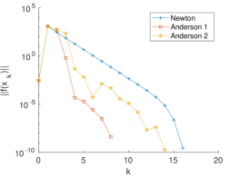
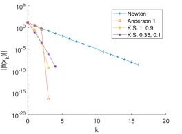
Figure 1: Left: convergence history for the trigonometric function (13), with $n=$10,000, for Newton and Newton-Anderson($m$), $m=1,2$. Right: convergence hisory for the Powell singular function (11), illustrating the high terminal order of convergence for Newton-Anderson(1).

For the trigonometric function (13), as $n$ increases, the Newton method has an extended preasymptotic regime of linear convergence. Both accelerated methods, which display superlinear (but subquadratic) convergence, attain residual tolerance in fewer iterations. Newton-Anderson($m$) for $m=1,2$ are illustrated for $n=$ 10,000, in figure 1 on the left. On the right of figure 1, the residual history for the Powell singular function is shown. The plot illustrates the curiously high approximate order of convergence for Anderson(1). The accelerated-Newton method is shown for comparison, with both sets of tested parameters, along with Newton.

Results for the Powell badly scaled function (9) are shown in table 2. For this problem, Newton-Anderson($m$) converges for $m>1$, but not $m=1$. Tests (not shown) were run for $m=1,\ldots,20$. However, as $n=2$ for this problem, the optimization problem reduces to a solvable linear system for depth $m=2$, and results with greater depths are not shown. Convergence can be restored for $m=1$ by applying a safeguarding strategy based on Lemma 2. If a Newton step is taken whenever $\cos(w_{k+1},w_{k})>0.942$, and the Anderson(1) step otherwise, then Newton-Anderson(1) converges, essentially tracking the Newton iteration.

2.2 Additional degenerate problems

Based on the results of [3], which show superlinear convergence of Newton-Anderson(1) to nonsimple roots of scalar equations, it is conjectured that Newton-Anderson also provides superlinear convergence to solutions of degenerate problems. Three such problems (in addition to the Powell singular function above) are collected in this section. The first two are standard problems from the literature and the third was chosen to demonstrate a case where Newton-Anderson(4) converges faster than Newton-Anderson($m$), for $m=1,2,3$.

1. From [6], $f:\mathbb{R}^{3}\rightarrow\mathbb{R}^{3}$

   $$f(x_{1},x_{2},x_{3})=\begin{pmatrix}x_{1}+x_{1}x_{2}+x_{2}^{2}\\ x_{1}^{2}-2x_{1}+x_{2}^{2}\\ x_{1}+x_{3}^{2}\end{pmatrix}\quad\text{ with }\,x_{0}=\begin{pmatrix}0.1,0.5,1.0\end{pmatrix}^{T}.$$ (17)

2. Chandrasekhar H-equation from [16]. The Chandrasekhar H-equation from radiative transfer (see [16, 26, 27] and the references therein), is given by

   $$F(H)(\mu)\coloneqq H(\mu)-\left(1-\frac{\omega}{2}\int_{0}^{1}\frac{\mu H(\nu)d\nu}{\mu+\nu}\right)^{-1}=0.$$

   Discretizing the equation (as described in [16, Example 2.10]) by the composite midpoint rule with $n$ subintervals, yields the discrete system in $f:\mathbb{R}^{n}\rightarrow\mathbb{R}^{n}$ given componentwise for $h\in\mathbb{R}^{n}=(h_{1},\cdots,h_{n})^{T}$, by

   $$f_{i}(h)=h_{i}-\left(1-\frac{\omega}{2n}\sum_{j=1}^{n}\frac{ih_{j}}{i+j-1}\right),\quad 1\leq i\leq n,\quad\text{ with }\,x_{0}=\begin{pmatrix}1,\ldots,1\end{pmatrix}^{T}.$$ (18)

3. Problem designed to demonstrate Newton-Anderson(4).

   $$f_{i}(x) =[(Ax-b)_{i}]^{p_{i}},~{}A=\begin{pmatrix}2&-1&\\ -1&2&-1\\ &\ddots&\ddots&\ddots\\ &&-1&2&-1\\ &&&-1&2\end{pmatrix},~{}b=\begin{pmatrix}-11,-7,-5,-3,-2,2,3,5,7,11\end{pmatrix}^{T},$$

   $$p=\begin{pmatrix}2,4,4,2,2,8,8,2,12,12\end{pmatrix},\quad\text{ with }\,x_{0}=\begin{pmatrix}0,\ldots,0\end{pmatrix}^{T}.$$ (19)

Problem	method	iterations ($k$)	$\|f(x_{k})\|$	$\|w_{k}\|$	$q_{k}$	time (sec)
D1.	Newton	14	3.991e-09	6.903e-05	1.077	0.000129
$n=3$	N. Anderson(1)	5	1.656e-10	1.349e-05	1.493	7.152e-05
	KS-acc. N. $(1.0,0.9)$	3	2.396e-09	0.0001877	1.993	4.476e-05
D2.	Newton	16	2.628e-09	0.000382	1.075	0.9698
$n=1000$	N. Anderson(1)	6	1.236e-11	0.001947	1.663	0.3671
	N. Anderson(2)	6	1.912e-11	2.595e-06	1.399	0.3658
	KS-acc. N. $(1.0,0.9)$	F	–	–	–	–
	KS-acc. N. $(0.35,0.1)$	4	3.986e-09	0.002449	1.461	0.4772
D3.	Newton	46	4.339e-09	0.07587	1.057	0.001038
$n=10$	N. Anderson(1)	17	7.899e-09	0.01347	1.45	0.0008288
	N. Anderson(2)	26	6.781e-11	0.0003507	1.404	0.002012
	N. Anderson(3)	6	3.964e-10	0.09431	5.87	0.000219
	N. Anderson(4)	5	7.289e-25	0.1056	23.05	0.0001861
	KS-acc. N. $(1.0,0.9)$	F	–	–	–	–
	KS-acc. N. $(0.35,0.1)$	F	–	–	–	–
	KS-acc. N. $(0.7,0.3)$	20	1.758e-09	0.07474	1.165	0.0007143

Table 3: Results for degenerate problems.

2.3 Discussion

In problems (17), (18), and (D3.), Newton-Anderson(1) converges faster than Newton by respective factors of 0.55, 0.38, and 0.8. Newton-Anderson(4) outperforms Newton-Anderson(1) by a factor of 0.22, and accelerated-Newton by a factor or 0.26, in the last problem. The approximate convergence order $q_{k}$ is close to one for Newton in each case, and greater than one (generally above 1.4) for each of the accelerated methods, when they converge. The accelerated-Newton method was run with an additional parameter pair for (D3.) as the method did not converge under either of the other two parameter-pairs used in the rest of the tests. The varied nature of these problems in terms of both problem dimension, and the dimension of the nullspaces at their respective solutions, indicates consistent behavior of Newton-Anderson on degenerate problems, which is worth a theoretical investigation.

The first problem (17) has a Jacobian featuring a two-dimensional nullspace at the solution. For the Chandrasekhar $H$-equation (18), the rank of the Jacobian at the solution is $n-1$. For the degenerate polynomial problem (D3.), the Jacobian has rank zero at the solution. The problem was designed to solve exactly for $m=4$ after the first full optimization. It is shown here to illustrate that there exists a class of problems for which $m>1$ is preferable. It is not yet clear what this problem class is.

3 Domain of convergence

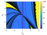
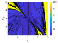
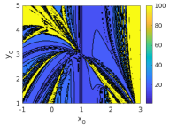
Figure 2: Domain of convergence to $x_{+}=x_{-}$ for (20) with $\varepsilon=0$. Left: Newton iterations; center: Newton-Anderson(1); right: accelerated-Newton with $C=0.5$ and $\alpha=0.35$.

In this section, the domains of convergence for Newton, Newton-Andreson(1), and accelerated-Newton are compared on standard benchmark degenerate and nearly degenerate polynomial systems.

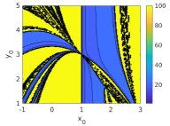
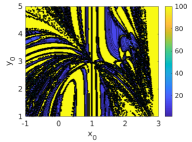
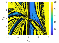
Figure 3: Domain of convergence to $x_{+}$ for (20) with $\varepsilon=10^{-6}$. Left: Newton iterations; center: Newton-Anderson(1); right: accelerated-Newton.

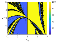
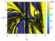
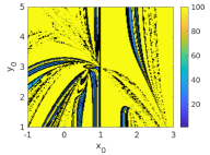
Figure 4: Domain of convergence to $x_{-}$ for (20) with $\varepsilon=10^{-6}$. Left: Newton iterations; center: Newton-Anderson(1); right: accelerated-Newton.

The first investigated problem is the polynomial system $f:\mathbb{R}^{2}\rightarrow\mathbb{R}^{2}$ from [8, Section 5].

$$f(x_{1},x_{2})=\begin{pmatrix}(x_{1}-1)+(x_{2}-3)^{2}\\ \varepsilon(x_{2}-3)+(3/2)(x_{1}-1)(x_{2}-3)+(x_{2}-3)^{2}+(x_{2}-3)^{3}\end{pmatrix}.$$ (20)

As presented in [8], for $\varepsilon>0$ there are two distinct roots in the vicinity of $x_{+}=(1,3)^{T}$, the second being $x_{-}=(1-\eta^{2},3+\eta)^{T}$, for $\eta=1-\sqrt{1+2\varepsilon}$. For $\varepsilon=0$, the degenerate case, the two roots coincide; and, for $\varepsilon\ll 1$ but $\varepsilon>0$, the near-degenerate case, the two roots are distinct but close. For figures 2-4, each algorithm is run from the the intial iterate $(x_{0},y_{0})$ for $x_{0}\in[-1,3]$ and $y_{0}\in[1,5]$ over a grid of 40,000 equally spaced points, and the number of iterations to convergence to a particular solution is displayed. The maximum of 100 iterations indicates not converging to the specified solution. As demonstrated in figure 2, Algorithm 2 has a similar domain of convergence to Newton (Algorithm 1) and accelerated-Newton, (Algorithm 4); but, as illustrated in figures 3-4, as $\varepsilon$ is varied away from zero, the Anderson method has substantially different domains of attraction to the roots $x_{-}$ and $x_{+}$. For this example, Algorithm 4 was run with parameters $C=0.5$ and $\alpha=0.35$, presented as optimal for $\varepsilon=10^{-6}$ in [8].

The second system investigated for domain of convergence is (17), from subsection 2.2. In this system, the Jacobian degenerates for coordinates $x_{3}=0$, and also for $x_{1}=x_{2}=0$. Here the domain of convergence is investigated for $x_{0}=(a,b,10^{-3})$, as the first two components are varied, again over a grid of 40,000 equally spaced initial iterates. This example points out that the domains of convergence are similar for the three algorithms, but the accelerated-Newton method is sensitive to parameter choice. With $\alpha$ and $C$ chosen small enough, the convergence is similar to Newton and Newton-Anderson, but with the parameters chosen too large ($C=1,\alpha=0.9$), the star-shaped domain of convergence is considerably smaller.

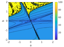
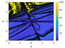
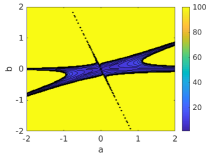
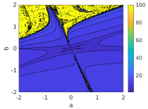
Figure 5: Domain of convergence to $x^{\ast}=(0,0,0)^{T}$ for (17), with $x_{0}=(a,b,10^{-3})^{T}$. Top left: Newton iterations; top right: Newton-Anderson(1); bottom left: accelerated-Newton with $C=1.0,\alpha=0.9$; bottom right: accelerated-Newton with $C=0.1,\alpha=0.35$.

4 Conclusion

This results of this numerical benchmarking investigation of the Newton-Anderson method indicate a superlinear but (usually) subquadratic order of convergence on both degenerate problems and nondegenerate problems. The superlinear convergence for nondegenerate problems is also shown theoretically. The Newton-Anderson method is seen to be advantageous in both the degenerate setting and for problems in which Newton’s method has an extended linearly converging preasymptotic regime, such as the trigonometric function (13) considered here. Further investigations show the method can show a similar domain of convergence to the standard Newton iteration for degenerate problems; however, under small perturbation of a problem parameter, the Newton-Anderson method may be attracted to a different solution than the Newton iteration.

References

- [1] S. Pollock, L. G. Rebholz, Anderson acceleration for contractive and noncontractive iterations, available as: arXiv:1810.08455 [math.NA] (2019).
- [2] C. Evans, S. Pollock, L. Rebholz, M. Xiao, A proof that Anderson acceleration improves the convergence rate in linearly converging fixed point methods (but not in those converging quadratically), available as: arXiv:1808.03971 [math.NA] (2019).
- [3] S. Pollock, Fast convergence to higher-multiplicity zeros (2019).
- [4] A. Quarteroni, R. Sacco, F. Saleri, Numerical Mathematics (Texts in Applied Mathematics), Springer-Verlag, Berlin, Heidelberg, 2006.
- [5] G. W. Reddien, On Newton’s method for singular problems, SIAM J. Numer. Anal. 15 (5) (1978) 993–996.
- [6] G. Reddien, Newton’s method and high order singularities, Computers & Mathematics with Applications 5 (2) (1979) 79–86. doi:https://doi.org/10.1016/0898-1221(79)90061-0.
- [7] C. Kelley, R. Suresh, A new acceleration method for Newton’s method at singular points, SIAM Journal on Numerical Analysis 20 (5) (1983) 1001–1009. doi:10.1137/0720070.
- [8] D. Decker, C. Kelley, Expanded convergence domains for Newton’s method at nearly singular roots, SIAM Journal on Scientific and Statistical Computing 6 (4) (1985) 951–966. doi:10.1137/0906064.
- [9] A. Griewank, On solving nonlinear equations with simple singularities or nearly singular solutions, SIAM Review 27 (4) (1985) 537–563.
- [10] J. J. Moré, B. S. Garbow, K. E. Hillstrom, Testing unconstrained optimization software, ACM Trans. Math. Softw. 7 (1) (1981) 17–41. doi:10.1145/355934.355936.
- [11] D. G. Anderson, Iterative procedures for nonlinear integral equations, J. Assoc. Comput. Mach. 12 (4) (1965) 547–560. doi:10.1145/321296.321305.
- [12] C. Kelley, A Shamanskii-like acceleration scheme for nonlinear equations at singular roots, Math. Comput. 47 (176) (1986) 609–623.
- [13] H. Fang, Y. Saad, Two classes of multisecant methods for nonlinear acceleration, Numer. Linear Algebra Appl. 16 (3) (2009) 197–221. doi:10.1002/nla.617.
- [14] H. F. Walker, P. Ni, Anderson acceleration for fixed-point iterations, SIAM J. Numer. Anal. 49 (4) (2011) 1715–1735. doi:10.1137/10078356X.
- [15] A. Toth, C. T. Kelley, Convergence analysis for Anderson acceleration, SIAM J. Numer. Anal. 53 (2) (2015) 805–819. doi:10.1137/130919398.
- [16] C. Kelley, Numerical methods for nonlinear equations, Acta Numerica 27 (2018) 207–287. doi:10.1017/S0962492917000113.
- [17] S. Pollock, L. Rebholz, M. Xiao, Anderson-accelerated convergence of Picard iterations for incompressible Navier-Stokes equations, SIAM J. Numer. Anal. 57 (2) (2019) 615–637. doi:10.1137/18M1206151.
- [18] J. Zhang, B. O’Donoghue, S. Boyd, Globally convergent type-I Anderson Acceleration for non-smooth fixed-point iterations, available as: arXiv:1808.03971 [math.OC] (2018).
- [19] M. J. D. Powell, A hybrid method for nonlinear equations, in: P. Rabinowitz (Ed.), Numerical Methods for Nonlinear Algebraic Equations, Gordon and Breach, New York, 1970, pp. 87–114.
- [20] R. Fletcher, M. J. D. Powell, A rapidly convergent descent method for minimization, The Computer Journal 6 (2) (1963) 163–168. doi:10.1093/comjnl/6.2.163.
- [21] M. J. D. Powell, An iterative method for finding stationary values of a function of several variables, The Computer Journal 5 (2) (1962) 147–151. doi:10.1093/comjnl/5.2.147.
- [22] J. S. Kowalik, M. R. Osborne, Methods for Unconstrained Optimization Problems, Vol. 13 of Modern analytic and computational methods in science and mathematics, Elsevier, New York, 1968.
- [23] K. M. Brown, A quadratically convergent Newton-like method based upon Gaussian elimination, SIAM J. Numer. Anal. 6 (4) (1969) 560–569. doi:10.1137/0706051.
- [24] C. G. Broyden, A class of methods for solving nonlinear simultaneous equations, Math. Comp. 19 (92) (1965) 577–593. doi:10.1090/S0025-5718-1965-0198670-6.
- [25] C. G. Broyden, The convergence of an algorithm for solving sparse linear systems, Math. Comp. 25 (114) (1971) 285–294. doi:10.1090/S0025-5718-1971-0297122-5.
- [26] I. W. Busbridge, The mathematics of radiative transfer., Cambridge tracts in mathematics and mathematical physics: no. 50, University Press, 1960.
- [27] S. Chandrasekhar, Radiative transfer., Engineering special collection, Dover Publications, 1960.