Precursors to plastic failure in a numerical simulation of CuZr metallic glass

Abstract

We deform, in pure shear, a thin sample of Cu₅₀Zr₅₀ metallic glass using a molecular dynamics simulation up to, and including, failure. The experiment is repeated ten times in order to have average values and standard deviations. Although failure occurs at the same value of the externally imposed strain for the ten samples, there is significant sample-to-sample variation in the specific microscopic material behavior. Failure can occur along one, two, or three planes, located at the boundaries of previously formed shear bands. These shear bands form shortly before failure. However, well before their formation and at external strains where plastic deformation just begins to be significant, non–affine displacement organizes itself along localized bands. The shear bands subsequently form at the edges of these non–affine–displacement–bands, and present an alternating rotation-quadrupole structure, as found previously by Şopu et al. [1] in the case of a notched sample loaded in tension. The thickness of shear bands is roughly determined by the available plastic energy. The onset of shear banding is accompanied by a sharp increase in the rate of change of the rotation angle localization, the strain localization, and the non–affine square displacement.

1 Introduction

Metallic glasses (MGs) and, particularly, bulk metallic glasses (BMGs) have been in existence since 1960 [2] and since 1993 [3, 4] respectively. They share a number of properties with oxide, and other, glasses, most notably the lack of long–range translational order. They differ, in that they are kept together not by covalent or ionic bonding but by metallic bonding, which does not have a preferred direction. This is an important ingredient leading to the fact that, in order to achieve a glassy state, melts have to be cooled quite rapidly in order to avoid crystallization [5]. The fact that BMGs can be mold–cast has enabled a number of applications for the fabrication of parts that need to have a prescribed shape and where a combination of high strength and low stiffness is useful. The fast cooling rate that is needed, however, severely limits their size.

The mechanical behavior of BMGs is a noteworthy characteristic that renders them unique [6]. At very low strains, their mechanical response is linear, similar to their crystalline counterparts. As the loading is increased however, crystalline metals develop dislocations and undergo plastic deformation. MGs, not having a crystal lattice, do not have this property and are, to a first approximation, brittle. This fact points to a fundamental question: how is one to link the microstructure of a MG with its macroscopic mechanical response? In crystals, this link is provided by the dislocations. Plastic flow does occur, though, in MGs, although to a much more limited extent than in crystals, and it is localized within thin shear bands (SBs) [7]. The appearance of SBs is often a signal of imminent failure, so it is critical to achieve as complete an understanding as possible of their behavior. Lacking the analytical tools that would be enabled by the existence of a crystalline structure, numerical simulation is the tool of choice to bridge the gap between the vastly different length scales that span the atomic to macroscopic domains.

Among the many existing MGs, one that has been the object of many studies, both experimental and numerical, is CuZr, with a variety of relative Cu contents, and with the possible addition of other elements such as Al [8, 9]. This interest stems from their superior glass forming ability [10], sensitivity of mechanical behavior to composition [11], and the existence of reliable interatomic potentials for numerical simulations [12, 13, 14]. In this sense, it has been possible to establish, for example, that the birth of multiple shear bands, induced by the presence of a crystalline phase in the glass matrix, avoids the fragile fracture and gives way to the formation of a plastic regime in the material [15]. In addition, the study of the nature of the shear transformation zones (STZs) and the interaction between them for the formation of SBs has been intensified.

Recently, Şopu et al. [1] have studied the growth of a SB in a notched specimen loaded in tension using molecular dynamics (MD) simulations. They have shown that a shear band is initiated, as expected, at the stress concentration due to the notch and propagates, also as expected, along a plane of maximum resolved shear stress. This propagation proceeds through a successive generation of vortex–like structures (associated with non–affine displacement (NAD)), and STZs. A study of the non–affine displacement field inside the SBs revealed the existence of these vortex–like structures, which represent the medium that transmits the distortion between STZs and that also have a high concentration of stress. They are, therefore, able to store enough energy to activate the next STZ. It was concluded that an adequate control over these “STZ–vortex” regions could lead to the control of the SB dynamics, perhaps avoiding instability.

Following previous work of us [16], in the present work we use MD simulations to study the generation of SBs in a Cu₅₀Zr₅₀ MG, paying special attention to the evolution of non–affine displacement. Rather than a notched specimen in tension, we consider a volume–conserving simple shear deformation in a sample that does not initially have any externally introduced flaws. Nevertheless, the mechanism of Ref. [1] appears to be, broadly, at work here as well, although in a different geometrical setting. In order to have proper averages and standard deviations of what is an essentially random behavior, we have repeated each numerical experiment ten times. We have studied the behavior of the NAD field, the local von Mises strain, local rotation angle and the local five–fold symmetry.

2 Simulation details

Molecular dynamics simulations for the Cu₅₀Zr₅₀ were carried out using LAMMPS software [17]. An embedded atom model (EAM) potential developed by Cheng et al. [18] was adopted to describe the interatomic interactions, which has been widely used to model Cu-Zr binary systems.

We build ten simulation samples, all of them consisting of 580 800 atoms, with dimensions of $80\times 40\times 2$ nm³. The reason for considering ten samples is discussed at the end of the paragraph. The reason for choosing one dimension much smaller than the other two is to facilitate the visualization of SBs. Each sample was made in the following way: We start with a FCC copper structure of 145 200 atoms and replace 50% of atoms by zirconium atoms at random positions. These systems are then heated from 300 K in the NPT ensemble for 2 ns up to 2 200 K and keeping a constant 0 GPa pressure. The integration timestep was set at 1 fs. Then, the molten metal is cooled down to 10 K following a procedure described by Wang et al. [19]. The estimated cooling rate is $10^{12}$ K$~{}\text{s}^{-1}$. This 145 200 atoms glass is replicated in $x$ and $y$ direction, followed by an equilibration in the NPT ensemble in order to remove eventual problems in the replication process, as described in [20]. Finally we let the system evolve in the NVE ensemble during 100 ps with a final minimization to ensure that all atomic forces were under $10^{-4}$ eV Å^-1, thus obtaining well–equilibrated metallic glass samples. Since each material sample is a single realization of a random material, we have repeated the procedure ten times in order to have conclusions that are reasonably representative of average properties and not just a statistical exception.

On these well–equilibrated samples we applied an engineering shear strain of $\dot{\gamma}=5\times 10^{8}$ s^-1, up to a maximum macroscopic deformation of $\gamma=0.20$. This is applied to the simulation cell in the $xy$ direction, using the NVE ensemble, and periodic boundary conditions (PBC) were set in all directions. When $\gamma=0.138\pm 0.006$, failure occurs. This is ascertained by the observed macroscopic displacement of one part of the sample relative to the other along a shear band. Although we continue the simulation, something that periodic boundary conditions allow us to do, up to $\gamma=0.20$ in order to ensure numerical stability, we are interested in the physics of the atomic processes leading up to failure.

2.1 Analytical tools

Several diagnostic tools were employed to analyze our simulations. The first is the von Mises strain invariant, commonly known as local atomic shear strain, $\eta^{\text{Mises}}$, proposed by Shimizu et al. [21]. This parameter is calculated by comparing two atomic configurations: current and reference, and computing the per–particle strain tensor $\eta^{i}_{\alpha\beta}$, as defined by the relative translation of its nearest neighbors:

$$\eta_{i}^{\text{Mises}}=\sqrt{(\eta_{yz}^{i})^{2}+(\eta_{xz}^{i})^{2}+(\eta_{xy}^{i})^{2}+\frac{(\eta^{i}_{yy}-\eta^{i}_{zz})^{2}+(\eta^{i}_{xx}-\eta^{i}_{zz})^{2}+(\eta^{i}_{xx}-\eta^{i}_{yy})^{2}}{6}}.$$ (1)

A global parameter that is a useful indicator of the overall sample behavior is the standard deviation of $\eta^{\text{Mises}}$ from its mean, the “degree of strain localization” [22] :

$$\psi=\sqrt{\frac{1}{N}\sum_{i=1}^{N}\left(\eta_{i}^{\text{Mises}}-\eta^{\text{Mises}}_{\text{ave}}\right)^{2}}\ ,$$ (2)

where $\eta_{\text{ave}}^{\text{Mises}}$ corresponds to the average value of the von Mises strain in the sample and $N$ is the total number of atoms. We have also computed the volumetric strain. Its magnitude, however, is two orders of magnitud smaller than the von Mises strain. Also, its behavior does not appear to shed additional light on the sample behavior so we will not discuss it further. The von Mises strain is the magnitude of the strain that is independent of volume change. As noted, it directly measures relative translations. We will consider a second descriptor that quantifies the rotation of an atom’s neighborhood, for each atom. This is obtained from the deformation gradient tensor $F$ as constructed by Zimmerman et al [23], for atomic systems. $F$ can be descomposed into the matrix product $F=RU$ of a rotation $R$ and a stretch $U$ [24]. The per–atom angle of rotation is calculated using the OVITO software [25]. Here we adopt a similar formula for the rotation angle localization, $\phi$, which we define as

$$\phi=\sqrt{\frac{1}{N}\sum_{i=1}^{N}\left(\theta_{i}-\theta_{\text{ave}}\right)^{2}}\ ,$$ (3)

where $N$ is the number of atoms, $\theta_{i}$ corresponds to the rotation angle for atom $i$ and $\theta_{\text{ave}}$ to the average of the rotation angle for all the atoms in the sample.

An important descriptor of amorphous material behavior at the mesoscopic scale is the non–affine displacement. That is, displacements that deviate from displacements that can be described by a linear strain field (see for example [26] and [27, 28]). We shall focus on non–affine displacements, and will introduce a global descriptor thereof, the mean non–affine square displacement of the sample,

$$\mathcal{R}^{2}_{\text{na}}\equiv\frac{1}{N}\sum^{N}_{i=1}\left|\vec{r}_{\text{na}}^{\;i}\right|^{2}\;,$$ (4)

where $\vec{r}_{\text{na}}^{\;i}$ corresponds to the non–affine displacement vector of the $i-th$ particle. This descriptor will be useful to characterize the strain at which shear bands are formed.

From an atomic structure point of view, it will be of interest to correlate changes in the non–affine displacement with the packing of the atomic structure. To do this, we shall use a Voronoi analysis [29], where we characterize each atom with its Voronoi indexes $\left<n_{3},n_{4},n_{5},n_{6}\right>$. With these Voronoi indices it is possible to define the local fivefold symmetry (L5FS) (Hu et al. [30]) as the number of pentagons in each polyhedron over the total number of faces that constitute it, that is

$$\text{L5FS}=\frac{n_{5}}{\sum_{i}n_{i}}\ .$$ (5)

This descriptor allows us to evaluate the stability of the atomic structure in MGs, as was previously described in [31, 32].

3 Results

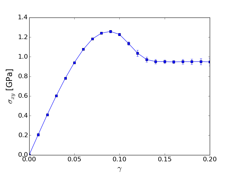
Figure 1: Averaged stress–strain curve of ten samples under simple shear deformation test. Error bars indicate the standard deviation. Non-affine displacement (NAD) begins to localize in homogeneous bands at about $\gamma\sim 0.7$. Shear bands (SBs) begin nucleating at about $\gamma\sim 0.10$. Failure occurs at $\gamma=0.14$. See text for details.

The ten samples were loaded in simple shear up to $\gamma=0.20$ as described in the previous section. Figure 1 shows the average stress–strain curve. There is linear elastic behavior only for small strains, up to $\gamma\sim 0.04$, with a shear modulus of $G=21.43$ GPa. Thereafter the curve bends downwards until reaching a maximum at $\gamma\sim 0.08$ with an ultimate tensile strength of $\sim 1.25$ GPa. There is little sample-to-sample variation as indicated by the small standard deviations. This behavior is in agreement with current understanding of amorphous materials: isolated STZs are generated at small strains [33, 34], and they provide an accumulating deviation from linear elasticity. At about $\gamma\sim 0.07-0.08$ serious plastic deformation sets in, and we shall focus on what happens within this region.

At about $\gamma\sim 0.12$ shear bands are fully identifiable, and the material fails at $\gamma=0.138\pm 0.006$. This is noticed as a sliding of the blocks adjacent to the SB along a “fault plane”. Although failure occurs at the same applied strain in all ten samples, the actual mechanism is different in each sample: It can occur along one fault plane only, or simultaneously along two or three fault planes. These fault planes coincide with boundaries of shear bands. After failure the numerical simulation can be continued due to the periodic boundary conditions. Here we defined a SB as regions with values of the von Mises strain above 0.3 and that completely cross the samples. Figure 2 shows the ten samples at $\gamma_{\text{max}}=0.20$ where the atoms are coloured according to their local von Mises strain, where the minimum is for purple at $\gamma=0.0$ and the maximum for yellow at $\gamma=0.6$. It is apparent that, although the global stress–strain behavior of the different samples is the same, their detailed evolution at the mesoscopic level is quite different: Strain is, as expected, localized in shear bands, as measured by the von Mises strain. There can be one, two or three bands, and they can point in any of the two directions of maximum shear stress.

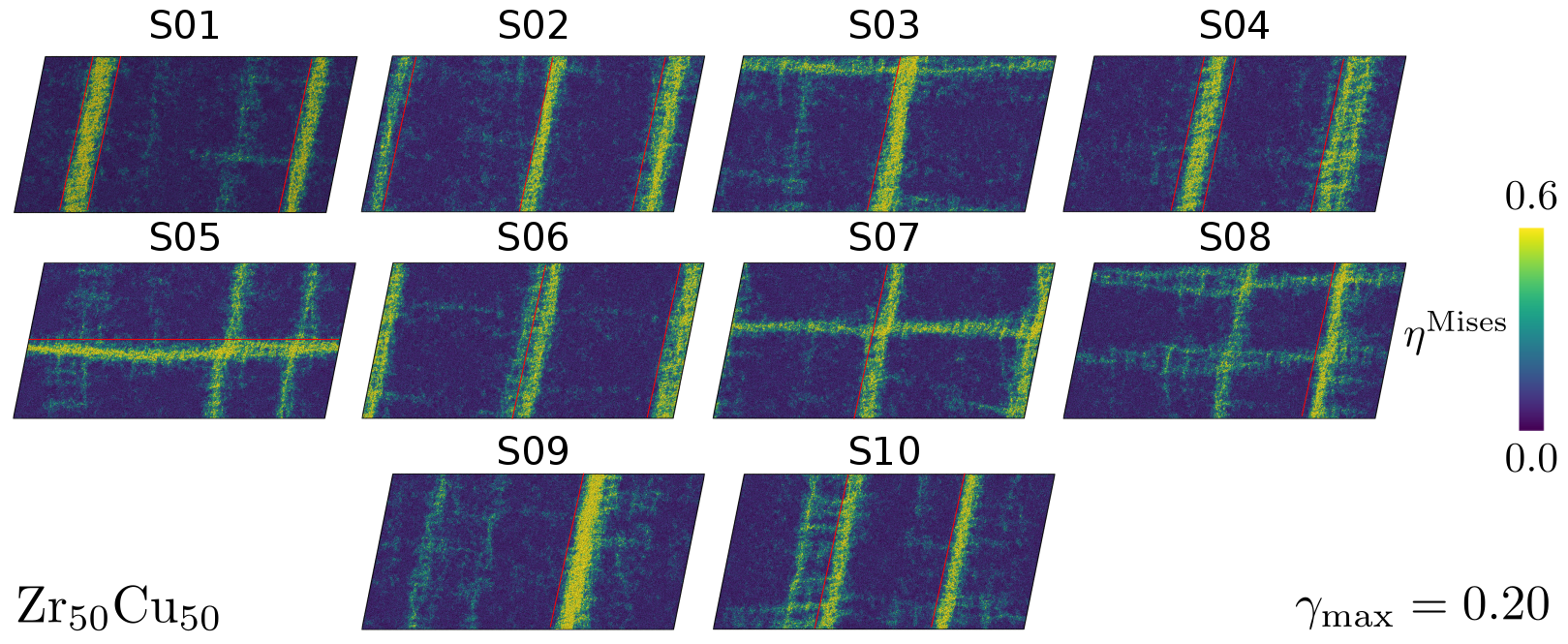
Figure 2: Von Mises strain $\eta^{\text{Mises}}$ at a strain of $\gamma=0.20$ for the ten Cu₅₀Zr₅₀ samples. Color indicates von Mises value. At $\gamma\approx 0.14$ all ten samples fail along one, two, or three surfaces (“fault planes”—FPs) located at the boundaries of shear bands, indicated by red lines. Samples S03, S07, S08 and S09 have one FP, samples S01, S04, S06 and S10 have two FPs and S02 and S05 have three FPs.

n

3.1 Local analysis

Figure 3 shows the evolution of both the non–affine displacement field and the von Mises strain of one sample in the whole material when the external shear $\gamma$ changes from 0.8 to 0.125. This is the strain interval where shear bands form and leads up to failure. In accordance with [26] we define the non–affine part of the displacement due to the external shear deformation as $\vec{r}_{\text{na}}=x_{\text{na}}\hat{x}+y_{\text{na}}\hat{y}$, where $x_{\text{na}}=x_{i}-\left(y_{i}/\dot{\gamma}\right)t-x_{0}$, $y_{\text{na}}=y_{i}-y_{0}$ and where $\dot{\gamma}$ is the shear rate, {$x_{i}$, $y_{i}$} the current coordinates of the particle $i$ and the reference coordinates {$x_{0},y_{0}$}. For the non–affine displacement field, shown as red arrows, we only display atoms whose NAD is above the mean at each stage of deformation. On the right panel we show those atoms that exhibit a von Mises strain $\eta^{\text{Mises}}\geq 0.3$.

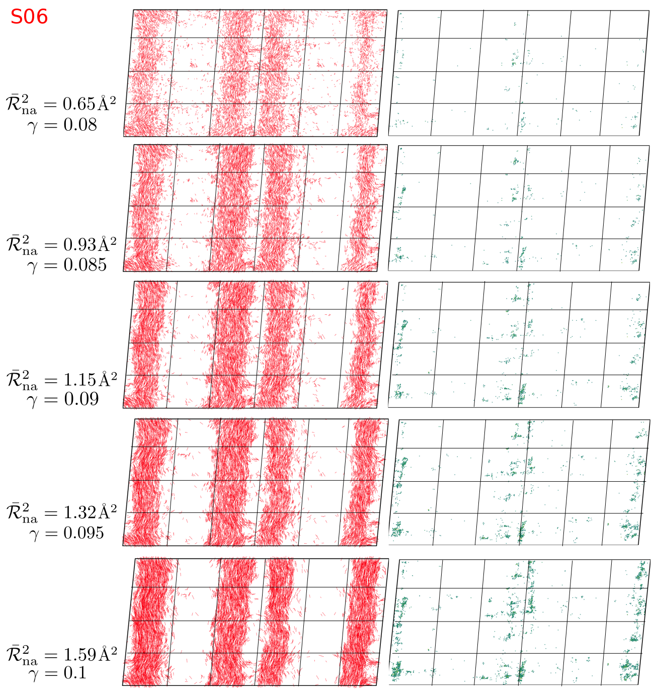
Figure 3: Behavior of non–affine displacement (NAD) and local von Mises strain in the region of plastic deformation leading up to failure. The left-hand panels show atoms with NAD bigger than average, whose value is indicated. The right-hand panels show atoms with von Mises strain greater than 0.3. NAD is localized along bounded regions well before shear banding starts. The latter activity does not overlap with the regions of high NAD. A grid is drawn to help visualized this NAD-SB avoidance. Shown here are the results for sample S06. All other samples behave in a similar fashion (not shown).

From the behavior of NAD and SB displayed on Figure 3 the following scenario emerges: First of all, the NAD organizes itself along narrow stripes that follow the directions of maximum resolved shear stress, and pointing along said directions, well before there is even a hint of shear banding. It is reasonable that NAD organizes in regions where it points roughly along the same direction, in order to minimize strain and hence to minimize energy. As external strain is increased, NAD is increased as well, and the displacement gradients, i.e., the internal stresses increase at the edges of the regions of high NAD. It is these extended regions that play the role of the notch in the numerical experiment of [1]. This generates a front, and all along this front regions of high von Mises strain, i.e., SBs, are formed. This scenario holds in the remaining nine samples as well (not shown).

The SB growth is limited because they consume a large amount of inelastic energy, so their thickness is limited. To verify this conclusion we perform an energy analysis of all the samples. First, as we perform the deformation of the system using the NVE ensemble, there exists an increase, on average, of the temperature up to $T\approx 57$ K. This increase only uses up about 1% of the available energy due to the externally applied stress. Second, to quantify the energy used to form the shear bands, we take the difference between the area under the stress–strain curve of the projected elastic behavior and the total stress–strain curve up to $\gamma=0.135$, as can be seen in figure 4. This will give us an energy per unit volume of each system under study. We compare this quantity with the energy per unit volume of the atoms that belong to the shear bands, defined as:

$$E_{r}=\frac{1}{2}\sum_{i\in\text{SBs}}^{N}\sigma_{xy}^{i}\cdot\eta^{xy}_{i}\;,$$ (6)

where $\sigma_{xy}^{i}$ are the components of the per–particle stress tensor of the $i-th$ atom, $\eta^{xy}_{i}$ the components of the per–particle strain tensor of the $i-th$ atom in the SBs. Here the Einstein sum rule is applied over the $x,y$ indices. Thus, $E_{r}$ will correspond to the energy used by the system to form the shear bands. As a result, taking the difference between the potential energy of the system and $E_{r}$ we obtain in average $0.063\pm 0.007$ eV Å^-3. Comparing with the result from the area under the stress–strain curve $E_{r}$, of $0.065$ eV Å^-3, we have a difference at the 3% level. This result supports our previous argument: the SBs consume a large amount of inelastic energy which limits their thickness. The average width of the shear bands of our simulations is $\sim 40$ Å.

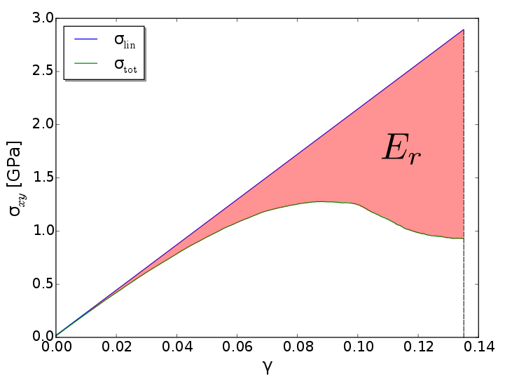
Figure 4: Difference between the area under the linear regime of stres–strain curve ($\sigma_{\text{lin}}$) and the total stress–strain curve ($\sigma_{\text{tot}}$) marked as $E_{r}$.This energy is absorbed by the shear bands and roughly determines their thickness.

As a result, SBs and regions of high NAD “avoid each other” and give rise to rotational motion in regions that comprise the SBs, as presented in figure 5. Here it is possible to identify a mechanism of deformation similar to the mechanism presented by Şopu et al. [1]: Within a SB, NAD is low, and there are regions with high rotational motion that alternate with regions of quadrupole–like displacement. In our case there is no externally generated flaw, so this alternation occurs, rather than sequentially along a propagating SB, homogeneously along the region occupied by the SB. To quantify this rotational motion we have calculated the rotation angle localization $\phi$ averaged over the 10 samples as well as its first and second derivative with respect to macroscopic strain $\gamma$. This is presented in figure 6(a). At $\gamma=0.10$, the onset of shear banding, there is a sudden, and significant (by a factor of four) acceleration in the rotation of the particles, as measured by the second derivative $d^{2}\phi/d\gamma^{2}$. This is followed by a deceleration of the rotation when the SBs are already consolidated at failure $\gamma=0.14$.

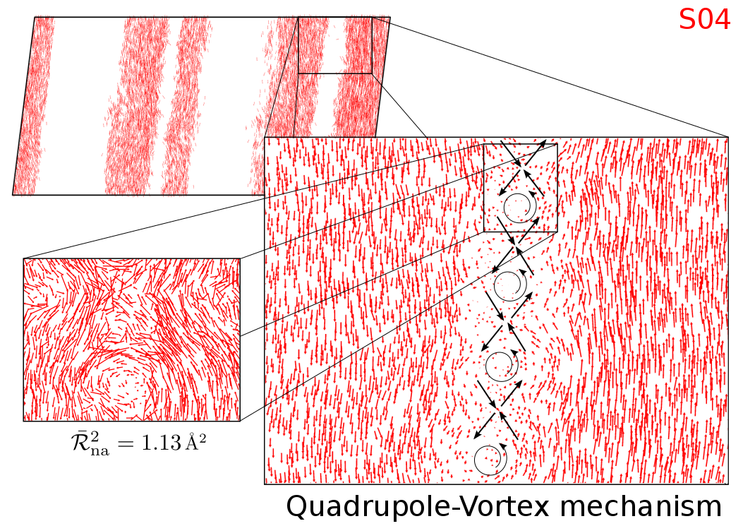
Figure 5: NAD for sample S04, at $\gamma=0.10$, where only atoms above the average are shown. The zoom corresponds to a complete NAD field, with alternating quadrupole–vortex regions. The same behavior obtains for all SBs in all samples (not shown).

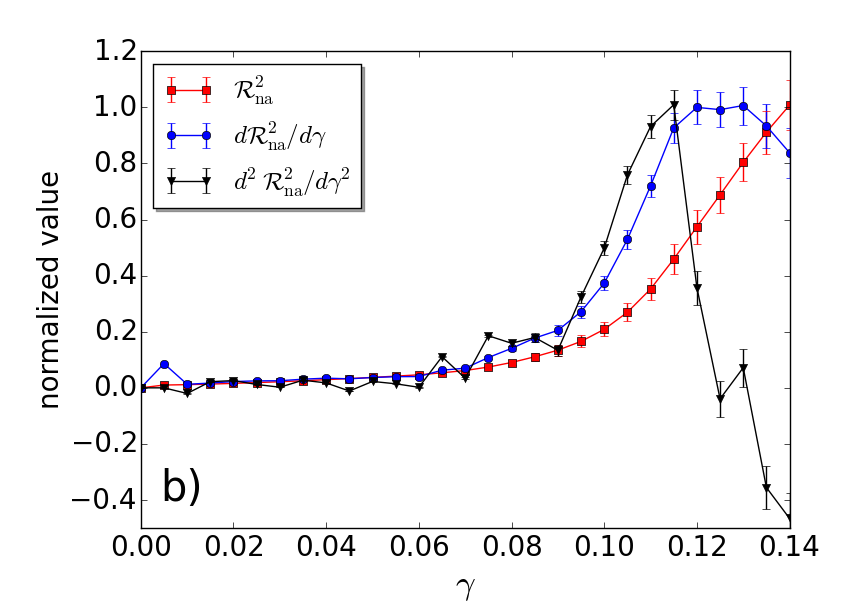
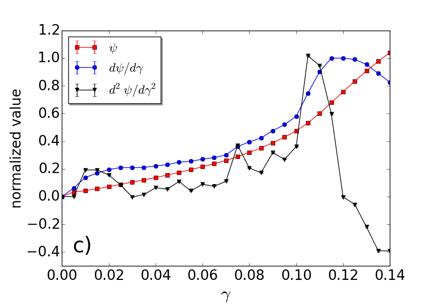
Figure 6: Normalized value of (a) averaged rotation angle localization $\phi$, (b) NAD $\mathcal{R}^{2}_{\text{na}}$ and (c) degree of strain localization $\psi$ with thier first and second derivatives as a function of macroscopic deformation $\gamma$.In all three cases, there is a sharp acceleration that coincides with the onset of shear banding at $\gamma\sim 0.10$. Each quantity is first computed as an average over a single sample. The result is then averaged over the ten samples. Error bars are the standard deviations in the latter averaging.

3.2 Global Analysis

Figure 6 shows, in addition to the behavior of the rotation angle localization $\phi$, two global parameters, the mean non–affine square displacement $\mathcal{R}^{2}_{\text{na}}$, Eq. (4), together with its first and second derivative, and the degree of strain localization $\psi$, Eq. (2), with its first and second derivative as well, as a function of external strain $\gamma$. All three quantities show an unmistakable acceleration, at $\gamma\sim 0.10$, when the shear banding sets in.

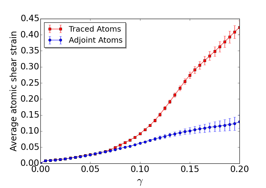
Figure 7: Average atomic shear strain for traced atoms, defined as atoms that experience a local von Mises strain grater than 0.3 after the shear band formation. Adjoint atoms represent the neighbors of traced atoms after the shear band is already formed. There is a sharp discontinuity in shear strain between the highly strained atoms (mostly belonging to shear bands) and their neighbors. Notice the accelerated rate of increase in shear strain from the beginning of plastic behavior ($\gamma\sim 0.7$) up to failure at $\gamma=0.14$.

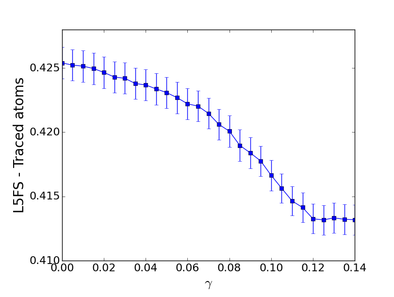
Figure 8: Averaged local five–fold symmetry (L5FS) for traced atoms as a function of macroscopic deformation. There is a steady decrease in the L5FS, with a slight increase in slope at the onset of plastic behavior at $\gamma\sim 0.7$, until shear bands are, roughly, fully formed at $\gamma\sim 0.12$. L5FS is then stabilized until failure at $\gamma=0.14$.

Further evidence that high stress is concentrated in localized patches is obtained focussing on atoms that, at the end of the simulation run, have $\eta^{\text{Mises}}\geq 0.3$. Following [32] we call them “traced atoms” and we compare the behavior of their number as a function of strain $\gamma$ with the behavior of their neighbors, called “adjoint atoms”. The result of this exercise is presented in figure 7, where the traced atoms show a change in the rate of increase of the atomic shear strain around $\gamma\sim 0.10$, similarly as the non–affine displacement field, $\mathcal{R}_{\text{na}}^{2}$, the rotation angle and the degree of strain localization $\psi$. As shown in the figure 6. The adjoint atoms, the neighbors to the highly strained ones, do not show this sharp increase in the second derivative.

Finally, the local five–fold symmetry has been linked in previous works, to the microscopic beahavior at the glass transition [29, 30] and within SBs [9]. In order to clarify the local structure of the shear band, we will focus our attention on the traced atoms and, as an indication of the local structure, we will calculate the local five–fold symmetry, L5FS, for those atoms. The results of L5FS for the traced atoms during the shear deformation tests are presented in the figure 8. The results of figure 8 indicate that the pentagonal structure of the traced atoms decreases during the formation of the shear band, and then stabilizes. The decrease, however, appears to be monotonous, although there appears to be some acceleration in the decrease of L5FS at $\gamma\sim 0.7$.

4 Discussion and Conclusions

Applying a uniform shear to ten samples of Cu₅₀Zr₅₀ MG we have found some interesting common features: First, their global behavior is very similar but their behavior at the atomic scale is very different, as they all fail at the same external strain, but their specific mechanism of failure differs from sample to sample. It can be along one, two, or three fault planes, that are at the boundary of shear bands. Second, there is a self-organization of non–affine displacement along localized bands, and this self-organization precedes and apparently triggers, the birth of shear bands. This fact, if it persists under conditions that differ from the conditions we have considered in the present numerical experiment, and in the absence of external flaws, could be an interesting candidate to play the role of precursor, to be closely monitored, to the nucleation of shear bands and subsequent failure. Third, the second derivative of several quantities (rotation angle localization, strain localization and non–affine square displacement) shows a sharp increase at onset of shear banding, preceding failure.

Our simulation has been carried out in shear, on a thin slab of Cu₅₀Zr₅₀ metallic glass at a temperature of 10 K, and at externally imposed strain rate of $\dot{\gamma}=5\times 10^{8}$ s^-1. It will be of interest to see if our conclusions hold for other values of the driving parameters, particularly temperature and strain rates. For example, Albe et al. [35] have used higher and lower strain rates for a tension test of Cu₆₄Zr₃₆ at 50 K and 300 K, and have uncovered a rich overall stress–strain behavior which it would be interesting to correlate with atomic–scale behavior.

References

- [1] Şopu D, Stukowski A, Stoica M, et al. Atomic–level processes of shear band nucleation in metallic glasses. Phys. Rev. Lett. (2017);119:195503.
- [2] Klement W, Williens RH, Duwez P. Non-crystalline structure in solidified gold–silicon alloys. Nature. (1960);187:869–870.
- [3] Peker A, Johnson WL. A highly processable metallic glass: Zr41.2Ti13.8Cu12.5Ni10.0Be22.5. Applied Physics Letters. (1993);63:2342–2344.
- [4] Inoue A, Horio A, Masumoto T. New amorphous Al–Ni–Fe and Al–Ni–Co alloys. Material Transactions, JIM. (1993);34:85–88.
- [5] Suryanarayana C, Inoue A. Bulk metallic glasses. CRC Press; (2011).
- [6] Hufnagel TC, Schuh CA, Falk ML. Deformation of metallic glasses: Recent developments in theory, simulations, and experiments. Acta Materialia. (2016);109:375 – 393.
- [7] Greer A, Cheng Y, Ma E. Shear bands in metallic glasses. Materials Science and Engineering: R: Reports. (2013);74:71 – 132.
- [8] Mei-Bo T, De-Qian Z, Ming-Xiang P, et al. Binary Cu–Zr bulk metallic glasses. Chinese Physics Letters. (2004);21:901–903.
- [9] Tercini M, de Aguiar Veiga RG, Zúñiga A. Local atomic environment and shear banding in metallic glasses. Computational Materials Science. (2018);155:129 – 135.
- [10] Xu D, Duan G, Johnson WL. Unusual glass-forming ability of bulk amorphous alloys based on ordinary metal copper. Phys Rev Lett. (2004);92:245504.
- [11] Kumar G, Ohkubo T, Mukai T, et al. Plasticity and microstructure of ZrCuAl bulk metallic glasses. Scripta Materialia. (2007);57:173 – 176.
- [12] Mendelev MI, Sordelet DJ, Kramer MJ. Using atomistic computer simulations to analyze x–ray diffraction data from metallic glasses. Journal of Applied Physics. (2007);102:043501.
- [13] Mendelev MI, Kramer MJ, Ott RT, et al. Development of suitable interatomic potentials for simulation of liquid and amorphous Cu–Zr alloys. Philosophical Magazine. (2009);89:967–987.
- [14] Borovikov V, Mendelev MI, King AH. Effects of stable and unstable stacking fault energy on dislocation nucleation in nano–crystalline metals. Modelling and Simulation in Materials Science and Engineering. (2016);24:085017.
- [15] Şopu D, Stoica M, Eckert J. Deformation behavior of metallic glass composites reinforced with shape memory nanowires studied via molecular dynamics simulations. Applied Physics Letters. (2015);106:211902.
- [16] Sepulveda-Macias M, Amigo N, Gutiérrez G. Onset of plasticity and its relation to atomic structure in cuzr metallic glass nanowire: A molecular dynamics study. Journal of Alloys and Compounds. (2016);655:357 – 363.
- [17] Plimpton S. Fast parallel algorithms for short–range molecular dynamics. Journal of Computational Physics. (1995);117:1–19.
- [18] Cheng Y, Ma E. Atomic–level structure and structure–property relationship in metallic glasses. Progress in Materials Science. (2011);56:379 – 473.
- [19] Wang C, Wong C. Structural properties of ZrxCu90-xAl10 metallic glasses investigated by molecular dynamics simulations. Journal of Alloys and Compounds. (2012);510:107 – 113.
- [20] Arman B, Luo SN, Germann TC, et al. Dynamic response of metallic glass to high–strain–rate shock loading: Plasticity, spall, and atomic–level structures. Phys. Rev. B. (2010) ;81:144201.
- [21] Shimizu F, Ogata S, Li J. Theory of Shear Banding in Metallic Glasses and Molecular Dynamics Calculations. Materials Transactions. (2007);48(11):2923 – 2927.
- [22] Cheng Y, Cao A, Ma E. Correlation between the elastic modulus and the intrinsic plastic behavior of metallic glasses: The roles of atomic configuration and alloy composition. Acta Materialia. (2009);57(11):3253 – 3267.
- [23] Zimmerman JA, Bammann DJ, Gao H. Deformation gradients for continuum mechanical analysis of atomistic simulations. International Journal of Solids and Structures. (2009);46(2):238 – 253.
- [24] Tucker GJ, Zimmerman JA, McDowell DL. Continuum metrics for deformation and microrotation from atomistic simulations: Application to grain boundaries. International Journal of Engineering Science. (2011);49(12):1424 – 1434.
- [25] Stukowski A. Visualization and analysis of atomistic simulation data with ovito–the open visualization tool. Modelling and Simulation in Materials Science and Engineering. (2010);18:015012.
- [26] Falk ML, Langer JS. Dynamics of viscoplastic deformation in amorphous solids. Phys Rev E. (1998);57:7192–7205.
- [27] Tanguy A, Wittmer JP, Leonforte F, et al. Continuum limit of amorphous elastic bodies: A finite–size study of low–frequency harmonic vibrations. Phys. Rev. B. (2002);66:174205.
- [28] Tanguy A, Leonforte F, Barrat JL. Plastic response of a 2D lennard–jones amorphous solid: Detailed analysis of the local rearrangements at very slow strain rate. The European Physical Journal E. (2006) ;20(3):355–364.
- [29] Jónsson H, Andersen HC. Icosahedral ordering in the lennard–jones liquid and glass. Phys. Rev. Lett. (1988);60:2295–2298.
- [30] Hu YC, Li FX, Li MZ, et al. Five-fold symmetry as indicator of dynamic arrest in metallic glass–forming liquids. Nature Communications. (2015);6:8310.
- [31] Wang Z, Sun BA, Bai HY, et al. Evolution of hidden localized flow during glass-to-liquid transition in metallic glass. Nature Communications. (2014);5:5823.
- [32] Tian ZL, Wang YJ, Chen Y, et al. Strain gradient drives shear banding in metallic glasses. Phys. Rev. B. (2017);96:094103.
- [33] Spaepen F. A microscopic mechanism for steady state inhomogeneous flow in metallic glasses. Acta Metallurgica. (1977);25(4):407 – 415.
- [34] Argon A. Plastic deformation in metallic glasses. Acta Metallurgica. (1979);27:47 – 58.
- [35] Albe K, Ritter Y, Şopu D. Enhancing the plasticity of metallic glasses: Shear band formation, nanocomposites and nanoglasses investigated by molecular dynamics simulations. Mechanics of Materials. (2013);67:94 – 103.