Spectra of Ni V and Fe V in the Vacuum Ultraviolet

Abstract

This work presents 97 remeasured Fe V wavelengths ($1200\text{\,}\mathrm{\SIUnitSymbolAngstrom}1600\text{\,}\mathrm{\SIUnitSymbolAngstrom}$) and 123 remeasured Ni V wavelengths ($1200\text{\,}\mathrm{\SIUnitSymbolAngstrom}1400\text{\,}\mathrm{\SIUnitSymbolAngstrom}$) with uncertainties of approximately $2\text{\,}\mathrm{m\SIUnitSymbolAngstrom}$. An additional 67 remeasured Fe V wavelengths and 72 remeasured Ni V wavelengths with uncertainties greater than $2\text{\,}\mathrm{m\SIUnitSymbolAngstrom}$ are also reported. A systematic calibration error is also identified in the previous Ni V wavelengths and is corrected in this work. Furthermore, a new energy level optimization of Ni V is presented that includes level values as well as Ritz wavelengths. This work improves upon the available data used for observations of quadruply ionized nickel (Ni V) in white dwarf stars. This compilation is specifically targeted towards observations of the G191-B2B white dwarf spectrum that has been used to test for variations in the fine structure constant, $\alpha$, in the presence of strong gravitational fields (Berengut et al., 2013). The laboratory wavelengths for these ions were thought to be the cause of inconsistent conclusions regarding the variation limit of $\alpha$ as observed through the white dwarf spectrum. These inconsistencies can now be addressed with the improved laboratory data presented here.

tablenum

1 Introduction

The development of unification theories that depend upon spatial and temporal variations of physical constants has and continues to be of interest to the physics community. Variations in the fine structure constant, $\alpha$, contribute to multiple cosmological models and string theories, as discussed by Martins (2017), such as the Bekenstein-Sandvik-Barrow-Magueijo theory (Sandvik, Barrow, & Magueijo, 2002; Barrow & Lip, 2012; Bekenstein, 1982). The search for variations in $\alpha$ has previously made use of methods involving both measurements based on atomic clocks (Berengut & Flambaum, 2012; Blatt et al., 2008; Bauch & Weyers, 2002) and on the observations of quasar spectra (Webb et al., 1999; Dzuba, Flambaum, & Webb, 1999) with the objective being ever finer limits on the potential variation.

The motivation behind our work stems from a recent publication that investigates the possible dependence of $\alpha$ on strong gravitational fields (Berengut et al., 2013). The study makes use of far-UV spectral observations of Fe V and Ni V in the atmosphere of the G191-B2B white dwarf star (Preval, Barstow, Holberg, & Dickinson, 2013). G191-B2B provides data for an analysis of the fine structure constant where the ions producing the observed spectrum experience a gravitational potential (relative to laboratory conditions) that is five orders of magnitude larger than in previous studies based on atomic clocks in Earth bound satellites. The analysis conducted by Berengut et al. (2013), however, resulted in conflicting estimates for $\Delta\alpha/\alpha$, which is demonstrated by Figures 1 and 2 of their paper. The laboratory wavelength standards for both Fe V and Ni V dominate the uncertainty of the fine structure variation.

The wavelength values used by Berengut et al. (2013) for Fe V were reported by Ekberg (1975). The reported wavelengths had estimated uncertainties of $4\text{\,}\mathrm{m\SIUnitSymbolAngstrom}$. This estimate of the wavelength uncertainty is supported by Berengut et al. (2013). Of the wavelengths reported by Ekberg, 96 were used in the investigation of fine structure variation covering a wavelength range of approximately $1200\text{\,}\mathrm{\SIUnitSymbolAngstrom}1600\text{\,}\mathrm{\SIUnitSymbolAngstrom}$.

In addition to the report by Ekberg, a rigorous assessment and optimization of Fe V data has been conducted by Kramida (2014). Kramida verified the uncertainty estimate given by Ekberg (1975) and used Ekberg’s data in conjunction with data from other researchers to derive a set of Fe V Ritz wavelengths with uncertainties of $2\text{\,}\mathrm{m\SIUnitSymbolAngstrom}$ or less.

The wavelengths for Ni V were reported by Raassen, van Kleef, & Metsch (1976, hereinafter RvKM76) and Raassen and van Kleef (1977, hereinafter RvK77). The reported wavelengths in the $200\text{\,}\mathrm{\SIUnitSymbolAngstrom}400\text{\,}\mathrm{\SIUnitSymbolAngstrom}$ range had estimated uncertainties of $1\text{\,}\mathrm{m\SIUnitSymbolAngstrom}$, but the wavelengths in the $900\text{\,}\mathrm{\SIUnitSymbolAngstrom}1400\text{\,}\mathrm{\SIUnitSymbolAngstrom}$ range were not reported with uncertainties. The uncertainties used in the report by Berengut et al. (2013) indicate that a $7\text{\,}\mathrm{m\SIUnitSymbolAngstrom}$ uncertainty seems to be appropriate. This estimated uncertainty is consistent with Raassen’s report on Ni VI (Raassen, 1980) that gives $6\text{\,}\mathrm{m\SIUnitSymbolAngstrom}$ as the estimated uncertainty in the $900\text{\,}\mathrm{\SIUnitSymbolAngstrom}1300\text{\,}\mathrm{\SIUnitSymbolAngstrom}$ range using the same calibration method as the one he used for Ni V. Of the wavelengths reported by RvK77, 32 were used in the investigation of fine structure variation covering a wavelength range of approximately $1200\text{\,}\mathrm{\SIUnitSymbolAngstrom}1400\text{\,}\mathrm{\SIUnitSymbolAngstrom}$.

2 Experimental Methods

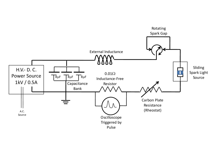
Figure 1: A diagram of the circuitry for the sliding spark light source.

The wavelengths in this work were measured with the National Institute of Standards and Technology (NIST) $10.7\text{\,}\mathrm{m}$ Normal Incidence Vacuum Spectrograph (NIVS), which operates in the $300\text{\,}\mathrm{\SIUnitSymbolAngstrom}5000\text{\,}\mathrm{\SIUnitSymbolAngstrom}$ range. The NIVS is in a Rowland Circle configuration that has a focal length of $10.7\text{\,}\mathrm{m}$ and contains a gold coated, concave grating blazed for $1200\text{\,}\mathrm{\SIUnitSymbolAngstrom}$ with $1200\text{\,}\mathrm{(grooves)}\text{\,}{\mathrm{mm}}^{-1}$. This results in a reciprocal linear dispersion $\approx$ $0.78\text{\,}\mathrm{\SIUnitSymbolAngstrom}\text{\,}{\mathrm{mm}}^{-1}$. The image recorded at the plate holder of the NIVS is created by a single slit with a width of $21\text{\,}\mathrm{\SIUnitSymbolMicro m}$.

The Ni V and Fe V spectra were obtained with a sliding spark source (Vodar & Astoin, 1950; Beverly, 1978; Reader, Epstein, & Ekberg, 1972). A diagram of the circuitry for the sliding spark is given in Figure 1. For this work we have used invar, an iron and nickel alloy, for both electrodes in the source. Invar was chosen in order to create exposures with both Ni V and Fe V in the same track. This allowed Ni V and Fe V to be placed on the same wavelength scale and ensured that any systematic errors in the calibration are common to both species. The exposures analyzed here were taken at a range of peak currents from $300\text{\,}\mathrm{A}$ to $2000\text{\,}\mathrm{A}$ with the best spectrum of Ni V and Fe V observed at a peak current of $1500\text{\,}\mathrm{A}$. In order to achieve that peak current, the inductor, shown in Figure 1, was removed from the spark circuitry. The carbon plate resistor contained thirteen carbon plates, the supply voltage was approximately $600\text{\,}\mathrm{V}700\text{\,}\mathrm{V}$ depending on the given exposure, the circuit spark gap was run at a repetition rate of $20\text{\,}\mathrm{ms}$, and the resulting pulse width was $50\text{\,}\mathrm{\SIUnitSymbolMicro s}$. The exposures were run for twenty minutes, and the average current was roughly $0.5\text{\,}\mathrm{A}$.

Table 1: Table of Spectra

Plate Number	Exposure Date	Plate Typea	Track Number	Sourceb	Source Conditions	$\lambda$ Range ($\AA$)
x988	07/03/2014	PIP	5	$D_{2}$	$300\text{\,}\mathrm{mA}$	$1150\text{\,}\mathrm{\SIUnitSymbolAngstrom}1450\text{\,}\mathrm{\SIUnitSymbolAngstrom}$
x990	07/11/2014	PIP	1	Pt/Ne HCL	$20\text{\,}\mathrm{mA}$, $340\text{\,}\mathrm{V}$	$1150\text{\,}\mathrm{\SIUnitSymbolAngstrom}1450\text{\,}\mathrm{\SIUnitSymbolAngstrom}$
x990	07/11/2014	PIP	4	Invar SS	$1000\text{\,}\mathrm{A}$ Peak, $0.55\text{\,}\mathrm{A}$ Average, $600\text{\,}\mathrm{V}$	$1150\text{\,}\mathrm{\SIUnitSymbolAngstrom}1450\text{\,}\mathrm{\SIUnitSymbolAngstrom}$
x990	07/11/2014	PIP	5	Invar SS	$1500\text{\,}\mathrm{A}$ Peak, $0.65\text{\,}\mathrm{A}$ Average, $850\text{\,}\mathrm{V}$	$1150\text{\,}\mathrm{\SIUnitSymbolAngstrom}1450\text{\,}\mathrm{\SIUnitSymbolAngstrom}$
x997	06/04/2015	KSWR	1	Pt/Ne HCL	$20\text{\,}\mathrm{mA}$, $310\text{\,}\mathrm{V}$	$1190\text{\,}\mathrm{\SIUnitSymbolAngstrom}1530\text{\,}\mathrm{\SIUnitSymbolAngstrom}$
x997	06/04/2015	KSWR	2	Invar SS	$1500\text{\,}\mathrm{A}$ Peak, $0.48\text{\,}\mathrm{A}$ Average, $530\text{\,}\mathrm{V}$	$1190\text{\,}\mathrm{\SIUnitSymbolAngstrom}1530\text{\,}\mathrm{\SIUnitSymbolAngstrom}$
x997	06/04/2015	KSWR	3	Fe/Y SS	$1500\text{\,}\mathrm{A}$ Peak, $0.45\text{\,}\mathrm{A}$ Average, $750\text{\,}\mathrm{V}$	$1190\text{\,}\mathrm{\SIUnitSymbolAngstrom}1530\text{\,}\mathrm{\SIUnitSymbolAngstrom}$
x997	06/04/2015	KSWR	4	Ni/Y SS	$1500\text{\,}\mathrm{A}$ Peak, $0.45\text{\,}\mathrm{A}$ Average, $750\text{\,}\mathrm{V}$	$1190\text{\,}\mathrm{\SIUnitSymbolAngstrom}1530\text{\,}\mathrm{\SIUnitSymbolAngstrom}$
x997	06/04/2015	KSWR	8	Pt/Ne HCL	$20\text{\,}\mathrm{mA}$, $310\text{\,}\mathrm{V}$	$1190\text{\,}\mathrm{\SIUnitSymbolAngstrom}1530\text{\,}\mathrm{\SIUnitSymbolAngstrom}$

The spectra were recorded on both Kodak SWR photographic plates and phosphor image plates. Table 1 presents the details for all exposures used in our work, and Figure 2 shows a sample from one of the spectra described in Table 1. The grain size in the photographic plates, roughly $0.5\text{\,}\mathrm{\SIUnitSymbolMicro m}$ (McCrea, 1971), gives the photographic plates a significant advantage over the other available VUV imaging techniques in terms of resolution and subsequent linewidth. The high density of spectral lines present in the invar spectrum makes the additional resolution provided by photographic plates necessary. Attempts to develop an accurate set of wavelengths with other imaging techniques, such as phosphor image plates, using the XGREMLIN software (Nave, Griesmann, Brault, & Abrams, 2015), were hindered by a significant number of blended lines.

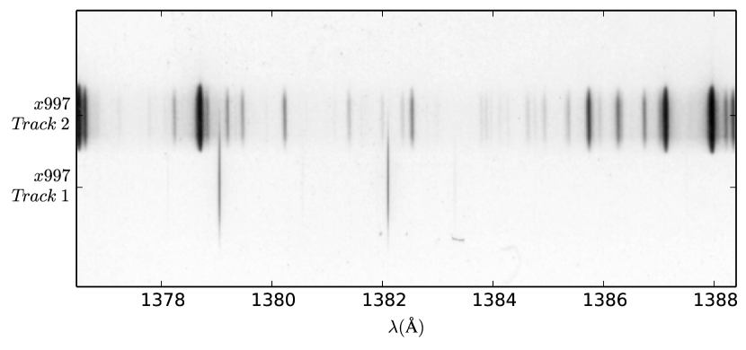
Figure 2: A sample section from the photographic plate x997, described in Table 1, that was used in our work to measure wavelengths. The top exposure is the spectrum of an invar SS source and the bottom exposuire is from a Pt/Ne HCL.

The wavelength scale for the invar spectrum recorded on photographic plates was calibrated with a Pt II spectrum produced with a platinum/neon hollow-cathode lamp (HCL) run with a current of $20\text{\,}\mathrm{mA}$. The Pt II spectrum was partially embedded in the invar spectrum without moving the photographic plates between the platinum and invar exposures (shown in Figure 2). This was done in order to eliminate the effects of moving the plates between the calibration spectrum and experimental spectrum. Attempts to apply a calibration derived from a separate track than the invar spectrum, that required vertically translating the plates, yielded a linear slope of spectrum along the plate. The sloping effects we observed are likely due to a tilting of the plates during the process of moving them vertically between separate exposures. When the plates were not moved between separate exposures the calibrated wavelengths of contaminant lines in the invar spectrum and the Fe V wavelengths that had available Ritz wavelengths were in much better agreement with their reported values.

The positions of the spectral lines present on the photographic plates were measured using the NIST rotating mirror comparator (Tomkins & Fred, 1951). The measurement uncertainty associated with the use of the NIST comparator was evaluated by taking multiple measurements of the same set of 83 well measured lines present in the invar spectrum and taking the standard deviation of the calibrated wavelengths that resulted from the line position measurements. The standard uncertainty introduced by the comparator measurement was determined to be $2\text{\,}\mathrm{m\SIUnitSymbolAngstrom}$ for lines without serious perturbations such as an asymmetry or blend. Lines with perturbations such as asymmetry or blending were given an increased measurement uncertainty, ranging from an additional $1\text{\,}\mathrm{m\SIUnitSymbolAngstrom}$ to $10\text{\,}\mathrm{m\SIUnitSymbolAngstrom}$, corresponding to the impact of the perturbation.

The radiometric calibration of the invar spectrum recorded on phosphor image plates was done with a deuterium standard lamp that was calibrated at the Physikalish-Technische Bundesanstalt (PTB). The $D_{2}$ spectrum, as well as the invar spectrum, was recorded on phosphor image plates for the radiometric calibration. We chose phosphor image plates for the radiometric calibration because they scale linearly with intensity (Nave, Sansonetti, Szabo, Curry, & Smillie, 2011), unlike the photographic plates which have a non-linear response in intensity.

3 Analysis

3.1 Calibration

3.1.1 Wavelength Calibration

The wavelength calibration for the Ni V and Fe V spectra was carried out with Pt II reference wavelengths (Sansonetti et al., 1992). Of the 93 platinum reference values used in the calibration of the invar spectrum, 59 of the wavelengths have uncertainties of less than $2\text{\,}\mathrm{m\SIUnitSymbolAngstrom}$ with the remaining values having uncertainties of $2\text{\,}\mathrm{m\SIUnitSymbolAngstrom}$.

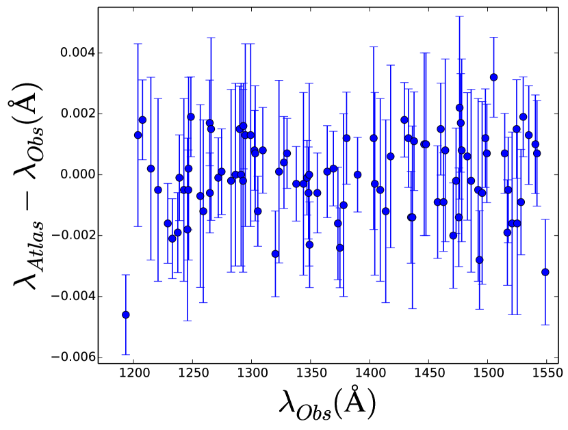
Figure 3: Residuals after fitting our observed Pt II wavelengths ($\lambda_{Obs}$) with a sixth order polynomial to their Pt II standard reference wavelengths ($\lambda_{Atlas}$) (Sansonetti et al., 1992).

The calibration function was created by identifying the positions on photographic plates of Pt II lines in the Pt/Ne spectrum that had wavelengths from Sansonetti et al. (1992). The line positions and reference wavelengths were then used to derive a dispersion function that was a sixth order polynomial. Once the dispersion function was determined, the line positions of Fe V, Ni V, and contaminant lines were measured and the polynomial dispersion function was applied. The contaminant lines, such as Y IV (Epstein & Reader, 1982) and Si IV (Griesmann & Kling, 2000), were then used to identify and correct illumination shifts between the calibration source (Pt/Ne HCL) and the experimental source (invar SS).

The standard uncertainty introduced due to the calibration, estimated by the standard deviation of the calibration residuals shown in Figure 3, is $1.3\text{\,}\mathrm{m\SIUnitSymbolAngstrom}$.

3.1.2 Intensity Calibration

With the $D_{2}$ spectrum discussed in section 2 we established an accurate intensity scale and report relative intensities for the observed Ni V lines. The approach to the radiometric calibration follows the same procedure discussed in section IV, subsection A of Nave, Sansonetti, Szabo, Curry, & Smillie (2011). Since the $D_{2}$ spectrum below $1660\text{\,}\mathrm{\SIUnitSymbolAngstrom}$ consists of emission lines, the peak intensity of the lines depends on the resolution of the spectrograph. As the resolution of the spectrograph used at PTB to calibrate the $D_{2}$ lamp was much lower than ours, we degraded our measured spectrum by convolving it with two boxcar functions of width $9.2\text{\,}\mathrm{\SIUnitSymbolAngstrom}$ and $4.6\text{\,}\mathrm{\SIUnitSymbolAngstrom}$ to match the resolution of the spectrograph used by PTB. We then interpolated the calibration provided by PTB to the same wavelength scale as our degraded spectra and took the ratio of the two spectra to create an instrument response function.

The instrument response function derived from this process was then applied to the invar spectrum by taking the ratio of the instrument response function and the invar spectrum signal. Each spectral line in the calibrated spectrum was fitted with a Voigt profile using the Xgremlin program (Nave, Griesmann, Brault, & Abrams, 2015). The peak value of the Voigt profile was taken as the line intensity of the spectral line.

The estimated uncertainty of the radiometric calibration is $12\text{\,}\mathrm{\char 37\relax}$ and was derived in a way that is similar to the uncertainty budget described in section IV, subsection B of Nave, Sansonetti, Szabo, Curry, & Smillie (2011). This uncertainty is a summation in quadrature of the $10\text{\,}\mathrm{\char 37\relax}$ uncertainty due to variations in the alignment of the source and the $7\text{\,}\mathrm{\char 37\relax}$ uncertainty that comes from the supplied calibration of the $D_{2}$ lamp from PTB. Since the line intensities are highly dependent on the source conditions and illumination, they are provided here as only a guide to the spectrum. Caution and great care should be used if the intensities are used for other purposes such as for calculating transition probabilities.

3.2 Wavelength Analysis

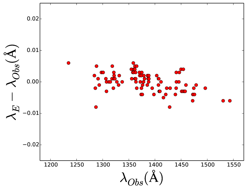
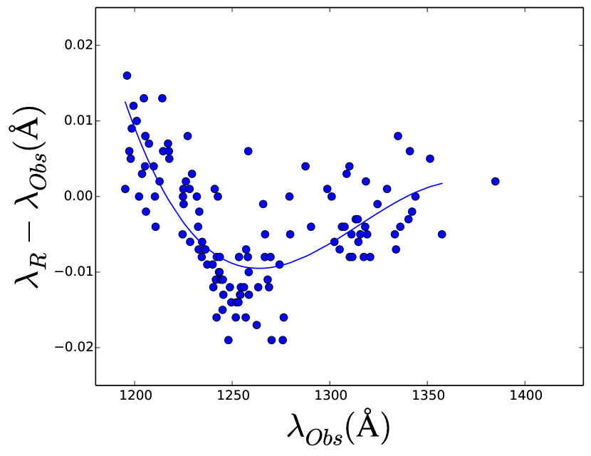
Figure 4: A comparison of the newly measured wavelengths ($\lambda_{Obs}$) to their previous values as reported by either Ekberg (1975) ($\lambda_{E}$) (Fe V) (Left) or RvK77 ($\lambda_{R}$) (Ni V) (Right). The uncertainty of each point is $5\text{\,}\mathrm{m\SIUnitSymbolAngstrom}$ (Left) and $7\text{\,}\mathrm{m\SIUnitSymbolAngstrom}$ (Right). The Ni V points (Right) are fitted by a third order polynomial shown by the solid line.

Figure 4 shows the comparison of the newly measured wavelength values to their previously reported values. Included are 97 of the 164 observed Fe V wavelengths and 123 of the 195 observed Ni V wavelengths. All included values are from unblended and symmetric lines. We excluded lines that were obscured by the calibration spectrum being partially embedded in the invar spectrum as a sufficiently accurate measurement of the line position was not possible. The excluded values are reported in seperate tables (2 and 4) with an increase in their reported uncertainties reflecting their perturbed measurements. The standard deviation of the difference in wavelengths shown in Figure 4 for Fe V is $3\text{\,}\mathrm{m\SIUnitSymbolAngstrom}$ and the standard deviation of the difference in wavelengths shown in Figure 4 for Ni V is $8\text{\,}\mathrm{m\SIUnitSymbolAngstrom}$.

For the observations of both Ni V and Fe V the reported standard uncertainties, $2.4\text{\,}\mathrm{m\SIUnitSymbolAngstrom}$, are the sum in quadrature of the calibration uncertainty discussed in 3.1.1 and the line position measurement uncertainty discussed in section 2.

An analysis of Figure 4 demonstrates the principle improvement found in our work. The Ni V comparison shown in the figure highlights a systematic difference between the newly measured wavelengths and the previous values from RvK77. This suggests a systematic error in the calibration method used by RvK77. This type of systematic error has been found previously in reports similar to RvK77. For example, in the work on the Co III spectrum by Smillie, Pickering, Nave, & Smith (2016) a similar trend was observed for wavelengths reported by Raassen & Ortin (1984).

The impact of correcting this systematic calibration error, concentrated in the $1200\text{\,}\mathrm{\SIUnitSymbolAngstrom}1300\text{\,}\mathrm{\SIUnitSymbolAngstrom}$ range, should be clear, given that the maximum error introduced by the faulty calibration is approximately $10\text{\,}\mathrm{m\SIUnitSymbolAngstrom}$, which would contribute significantly to any application requiring Ni V wavelengths. The maximum discrepancy in Figure 2 of Berengut et al. (2013) is roughly $12\text{\,}\mathrm{m\SIUnitSymbolAngstrom}$, suggesting that the majority of the discrepancy they observed can by explained by the laboratory wavelengths.

Table 2: Compilation of Ni V Data

$\lambda_{obs}$ a	$u_{obs}$ b	$\lambda_{Ritz}$ c	$u_{Ritz}$ d	I e	$\log(gf_{R})$ f	$\log(gf_{R})$ g	$E_{i}$ h	$E_{k}$ i	Lower Level			Upper Level			Notes j
($\mathrm{\SIUnitSymbolAngstrom}$)	($\mathrm{\SIUnitSymbolAngstrom}$)	($\mathrm{\SIUnitSymbolAngstrom}$)	($\mathrm{\SIUnitSymbolAngstrom}$)	Acc.			($\mathrm{cm}$-1)	($\mathrm{cm}$-1)	Configuration	Term	J	Configuration	Term k	J
199.1540	0.0019	199.1540	0.0019	41			0.00	502124.0	3d6	5D	4	3d5(6S)5f	5F°	5	R2
199.5040	0.0019	199.5040	0.0019	37			889.61	502132.7	3d6	5D	3	3d5(6S)5f	5F°	4	R2
		…
1003.233	0.022	1003.2499	0.0031	27	-1.057	E	217049.7	316725.76	3d5(4G)4s	3G	5	3d5(2H)4p	3G°	5	R4
1008.269	0.022	1008.2699	0.0056	14	-1.317	E	217100.94	316280.73	3d5(4G)4s	3G	3	3d5(2F1)4p	3F°	3	d,R4
		…
1187.168	0.025	1187.2012	0.0029	2	-1.496	E	235421.42	319653.14	3d5(2F1)4s	3F	4	3d5(4F)4p	3G°	5	d,R3
1187.770	0.025	1187.7953	0.0048	35	-1.249	E	208164.06	292353.65	3d5(4G)4s	5G	4	3d5(4G)4p	3H°	5	p,R3
		…
1201.752	0.022	1201.7557	0.0056	46	-1.043	E	263701.48	346913.07	3d5(2D2)4s	3D	1	3d5(2D2)4p	3P°	2	d,bl,R1
1201.849	0.022	1201.8470	0.0084	29	-0.784	E	247165.79	330371.06	3d5(2F2)4s	3F	2	3d5(2S)4p	3P°	1	p,R1
		…
1228.167	0.002	1228.1685	0.0016	100	-0.810	E	242504.64	323926.69	3d5(2G2)4s	3G	4	3d5(2H)4p	3H°	4	I,W
1228.432	0.002	1228.4291	0.0015	20	-0.129	E	242504.64	323909.42	3d5(2G2)4s	3G	4	3d5(2G2)4p	3H°	5	I,W

Note. — Table 2 is published in its entirety in the electronic edition of the Astrophysical Journal.

4 Results

We have combined our work with the corrected wavelengths from RvKM76 and RvK77, described in section 4.1.2, and used them to derive optimized energy levels and Ritz wavelengths. Table 2 provides the full results of our compilation for Ni V. Columns 1 and 2 give observed wavelengths and their standard uncertainties as described in sections 3.2 and 4.1.2. Columns 3 and 4 give Ritz wavelengths, derived from the optimized energy levels, and their standard uncertainties as described in section 4.4. Column 5 gives the relative intensity of the line as described in sections 3.1.2 and 4.2. Columns 6 and 7 give the $\log(gf)$ values of each transition as well as the estimated standard uncertainty of each $\log(gf)$ value as described in section 4.3. Columns 8 and 9 give the lower and upper optimized energy levels for each transition as described in section 4.4. Columns 10 through 15 give the lower and upper configuration, term, and J value of each transition. Column 16 provides additional notes for each transition with each note character being described in the footer of Table 2.

4.1 Wavelengths

4.1.1 Fe V

In addition to comparisons with the values from Ekberg (1975), we have also compared our results to the Ritz values from Kramida (2014). In almost all cases the two sets of wavelengths agree with each other to within one standard uncertainty. Overall the two reports support each other, which can be clearly seen in figure 5, which shows a standard deviation of $7\text{\,}\mathrm{m\SIUnitSymbolAngstrom}$ in the difference between the two sets. Figure 5 does show a small sloping trend in the difference between the two sets of wavelengths towards longer wavelengths. This indicates that there is still a small systematic error in one of the sets of wavelengths, but the sloping trend in figure 5 shows that the remaining systematic error is small relative to the wavelength uncertainties.

Figures 4 and 5 show that no substantial improvements have been made for Fe V as a result of the new measurements reported in this work. Our measurements do, however, validate the wavelengths reported by Ekberg (1975) and Kramida (2014). Ultimately, the assessment of Fe V by Kramida (2014) stands as the recommended source of reference data for Fe V.

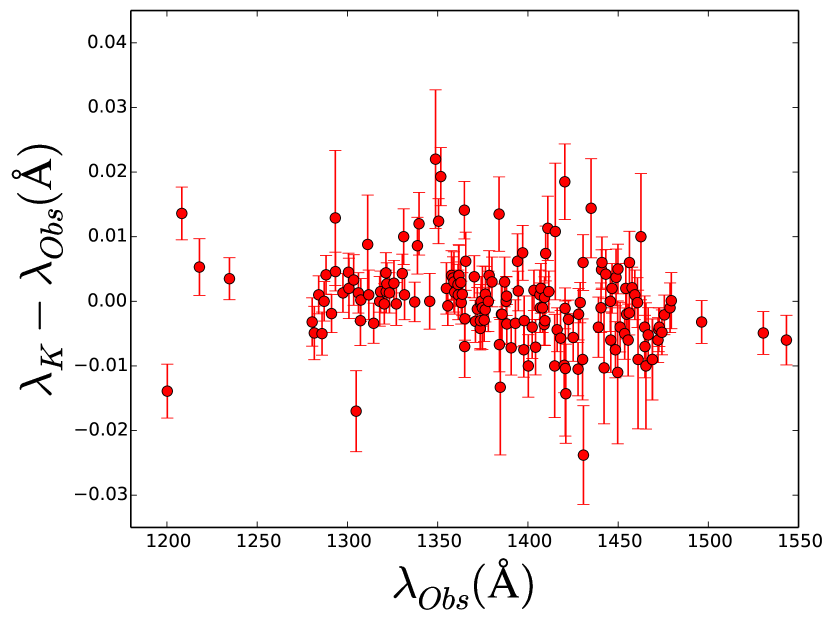
Figure 5: A comparison of the new Fe V wavelengths ($\lambda_{Obs}$) to the Ritz wavelengths ($\lambda_{K}$) from Kramida (2014).

4.1.2 Ni V

The reports by RvK77 and RvKM76 span a wavelength range of $200\text{\,}\mathrm{\SIUnitSymbolAngstrom}1400\text{\,}\mathrm{\SIUnitSymbolAngstrom}$ and include approximately 1500 spectral lines. Roughly 300 of the lines that fall between $1200\text{\,}\mathrm{\SIUnitSymbolAngstrom}1400\text{\,}\mathrm{\SIUnitSymbolAngstrom}$ were not remeasured in our work. The wavelengths for these lines can be corrected by shifting them to the same wavelength scale as the newly remeasured wavelengths. This was done by fitting the points in Figure 4 with a third order polynomial. The standard deviation of the residuals of the third order polynomial fit shown for Ni V in figure 4 is $5\text{\,}\mathrm{m\SIUnitSymbolAngstrom}$. This was then applied to the wavelengths reported by RvK77 in the $1200\text{\,}\mathrm{\SIUnitSymbolAngstrom}1300\text{\,}\mathrm{\SIUnitSymbolAngstrom}$ region to give wavelengths on our new scale. The wavelengths in Table 2 that have been corrected in this way are reported as the observed wavelengths with a mark (R1) in the note column.

In the wavelength region that did not overlap with the remeasured wavelengths, the accuracy of the wavelength scale can be examined using Ritz wavelengths. Accurate relative values of the $3d^{5}4p$ levels were derived from $3d^{5}4s$-$3d^{5}4p$ transitions in the $1200\text{\,}\mathrm{\SIUnitSymbolAngstrom}1400\text{\,}\mathrm{\SIUnitSymbolAngstrom}$ range using the level optimization program LOPT described in more detail in section 4.4. The relative values and uncertainties of the $4p$ levels are determined solely by lines in the $1200\text{\,}\mathrm{\SIUnitSymbolAngstrom}1400\text{\,}\mathrm{\SIUnitSymbolAngstrom}$ region. The absolute values are set by fixing the value of one level in the optimization. The $3d^{5}4p$ levels combine with each level in the $3d^{6}$ configuration to give transitions in the $300\text{\,}\mathrm{\SIUnitSymbolAngstrom}400\text{\,}\mathrm{\SIUnitSymbolAngstrom}$ region. The relative Ritz wavelengths and uncertainties of transitions down to a single $3d^{6}$ level are determined by lines in the longer wavelength region and can be compared to the measured values from RvKM76 to evaluate the accuracy of their wavelength scale by looking for systematic deviations. For example, the $3d^{6}$ ${}^{3}P_{2}$ level at $262\,152\text{\,}{\mathrm{cm}}^{-1}$ combines with $3d^{5}4p$ levels to give 25 lines from $329.25\text{\,}\mathrm{\SIUnitSymbolAngstrom}382.37\text{\,}\mathrm{\SIUnitSymbolAngstrom}$. A systematic deviation from a constant value in the difference between the measured and Ritz wavelengths for these lines would suggest a problem in the relative wavelengths in RvKM76. This technique does not validate the absolute wavelength calibration as the absolute values of the $4p$ levels must be determined by at least one $3d$-$4p$ transition, but can determine if a wavelength calibration error similar to that shown in figure 4 exists in the shorter wavelength region.

In our case, it was necessary to fix the values of two $3d^{5}4s$ energy levels in the level optimization in order to provide values for a sufficient number of $4p$ levels to determine Ritz wavelengths across the whole $300\text{\,}\mathrm{\SIUnitSymbolAngstrom}400\text{\,}\mathrm{\SIUnitSymbolAngstrom}$ wavelength range. The $3d^{5}(^{4}D)4s$ ${}^{5}D_{2}$ level was set at $216\,590.519\text{\,}{\mathrm{cm}}^{-1}$ and the $3d^{5}(^{2}I)4s$ ${}^{1}I_{6}$ level at $233\,840.023\text{\,}{\mathrm{cm}}^{-1}$ using an initial optimization of all lines in the $200\text{\,}\mathrm{\SIUnitSymbolAngstrom}1400\text{\,}\mathrm{\SIUnitSymbolAngstrom}$ wavelength range. Values for 21 levels in the $3d^{6}$ configuration were then fixed using single $3d$-$4p$ transitions and Ritz wavelengths for $3d$-$4p$ transitions calculated using the fixed $3d^{6}$ levels and optimized $3d^{5}4p$ levels. The results of this comparison, shown in Figure 6, indicate no calibration error in the $300\text{\,}\mathrm{\SIUnitSymbolAngstrom}400\text{\,}\mathrm{\SIUnitSymbolAngstrom}$ range as there is no systematic behavior, and the scatter in the difference between the wavelengths is within the estimated measurement uncertainty. From this assessment we have reported the original wavelengths in Table 2 in the $300\text{\,}\mathrm{\SIUnitSymbolAngstrom}400\text{\,}\mathrm{\SIUnitSymbolAngstrom}$ range given by RvKM76 with a mark (R2) in the note column.

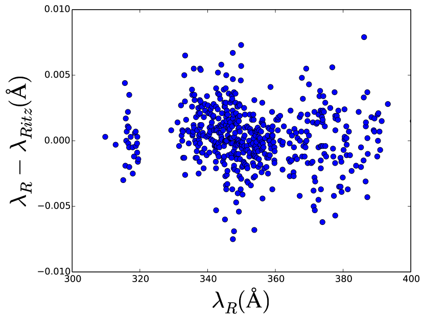
Figure 6: A comparison of the wavelengths reported by RvKM76 ($\lambda_{R}$) to the Ritz wavelengths described above ($\lambda_{Ritz}$).

In the $900\text{\,}\mathrm{\SIUnitSymbolAngstrom}1200\text{\,}\mathrm{\SIUnitSymbolAngstrom}$ range, we took a similar approach. The optimized energy levels used to evaluate the $300\text{\,}\mathrm{\SIUnitSymbolAngstrom}400\text{\,}\mathrm{\SIUnitSymbolAngstrom}$ range were the upper and lower energy levels of most of the transitions in the $900\text{\,}\mathrm{\SIUnitSymbolAngstrom}1200\text{\,}\mathrm{\SIUnitSymbolAngstrom}$ range. We used these levels to calculate Ritz wavelengths to compare to the wavelengths reported by RvKM76. The comparison, shown in Figure 7, demonstrated that the calibration error trend seen in the $1200\text{\,}\mathrm{\SIUnitSymbolAngstrom}1300\text{\,}\mathrm{\SIUnitSymbolAngstrom}$ range (shown in Figure 4) continued down towards $1100\text{\,}\mathrm{\SIUnitSymbolAngstrom}$. We corrected the wavelengths in the $1100\text{\,}\mathrm{\SIUnitSymbolAngstrom}1200\text{\,}\mathrm{\SIUnitSymbolAngstrom}$ range by shifting down the wavelengths reported by RvKM76 by $11\text{\,}\mathrm{m\SIUnitSymbolAngstrom}$ (the average of the differences between the Ritz wavelengths and the wavelengths reported by RvKM76). We increased the uncertainty of these wavelengths by the standard deviation of the set of differences ($12\text{\,}\mathrm{m\SIUnitSymbolAngstrom}$). This $12\text{\,}\mathrm{m\SIUnitSymbolAngstrom}$ correction was added to the original measurement uncertainty of each wavelength as a sum in quadrature. The wavelengths in Table 2 that have been corrected in this way are reported as the observed wavelengths with a mark (R3) in the note column.

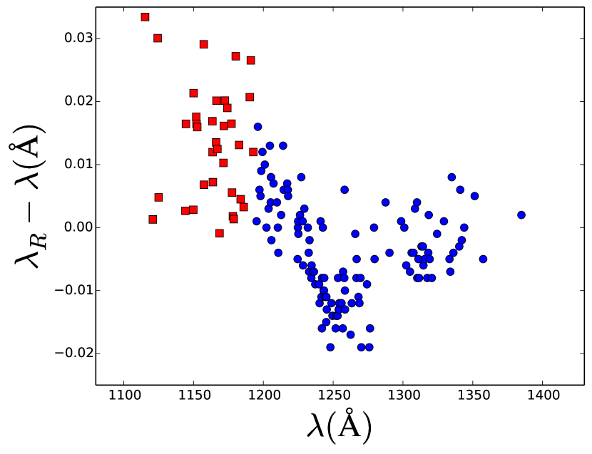
Figure 7: A comparison of the wavelengths reported by RvK77 ($\lambda_{R}$) to our newly measured wavelengths ($\lambda$) (blue circles) and to the Ritz wavelengths described in section 4.1.2 ($\lambda$) (red squares). The two comparisons, when joined together, show that the calibration error described in section 3.2 extends into the shorter wavelength region shown with the red squares.

The wavelengths in the $900\text{\,}\mathrm{\SIUnitSymbolAngstrom}1100\text{\,}\mathrm{\SIUnitSymbolAngstrom}$ range and the $1300\text{\,}\mathrm{\SIUnitSymbolAngstrom}1400\text{\,}\mathrm{\SIUnitSymbolAngstrom}$, similar to those in the $300\text{\,}\mathrm{\SIUnitSymbolAngstrom}400\text{\,}\mathrm{\SIUnitSymbolAngstrom}$ range, did not demonstrate any systematic errors, so we have given them in Table 2 as the original values given by RvK77 with a mark (R4) in the note column.

4.2 Intensity

The line intensities in column five of Table 2 were taken from our spectra when available. If an accurate intensity could not be determined from our spectra due to issues with fitting the line profile, which could occur as a result of blending or having a weak line on the shoulder of stronger lines, then the line includes a characteristic mark in Table 2 indicating an unreliable intensity value.

As not all of the lines reported by RvK77 and RvKM76 were measured in this work, the line intensities reported in Table 2 are on two scales. Lines that have updated intensity measurements through this work are on the calibrated scale, while lines that were not measured in this work are reported on the original scale set by RvK77 and RvKM76. Table 2 includes a clear marker in the note column on each entry to indicate if the line intensity is from the original (noted as R) or updated scale (noted as W).

4.3 $\log(gf)$

The $\log(gf)$ values presented in Table 2 are the result of detailed calculations carried out by Raassen & Uylings (1996). The accuracy of those $\log(gf)$ values was assessed by comparing them to the $\log(gf)$ values calculated by Kurucz (1977). Figure 8 presents the difference of the two sets as a function of the calculated line strength values given in atomic units (a.u.):

$$a_{0}^{2}e^{2}=$2.729\text{\times}{10}^{-48}\text{\,}{\mathrm{m}}^{2}\text{\,}{\mathrm{C}}^{2}$$$ (1)

where $a_{0}$ is the Bohr radius and $e$ is the electric charge. The plot in Figure 8 has a standard deviation of $0.3$.

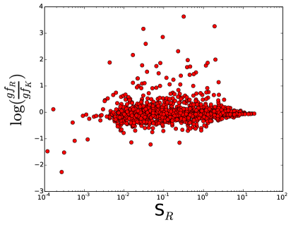
Figure 8: Difference between the $\log(gf)$ values reported by Raassen & Uylings (1996) ($\log(gf_{R})$) and Kurucz (1977) ($\log(gf_{K})$) as a function of line strengths calculated using values from Raassen & Uylings (1996) ($S_{R}$). The line strengths are given in atomic units defined by eqautaion 1.

Historically, the calculations provided by Raassen & Uylings (1996) have been far more accurate than other calculations (Fuhr & Wiese, 2006) and so the uncertainties for the $\log(gf)$ values provided by Raassen & Uylings (1996) can be roughly estimated by taking the standard deviation of the difference of the two sets of $\log(gf)$ values as a function of the line strengths calculated by Kurucz (1977). This results in a conservative upper limit for the $\log(gf)$ uncertainties reported in Table 2. Ultimately, the uncertainties for the $\log(gf)$ values were broken down into three levels of quality based on the line strength. The weakest lines ($S$ $\leq$ 5 a.u.) have the lowest rating (uncertainty $>$50\text{\,}\mathrm{\char 37\relax}$$), moderate lines ( 5 a.u. $<S\leq$ 10 a.u.) have the middle rating (uncertainty $\leq$18\text{\,}\mathrm{\char 37\relax}$$), and the strongest lines ($S>$ 10 a.u.) have the highest rating (uncertainty $\leq$7\text{\,}\mathrm{\char 37\relax}$$). These different uncertainty levels are given in column seven of Table 2.

4.4 Level Optimization

Table 3: Energy Levels of Ni V

Configuration	Term a	J	Energy	$u_{E}$ b	Number of Transitions
			($\mathrm{cm}$-1)	($\mathrm{cm}$-1)	Determining Level
3d6	5D	4	0.00	0.00	33
3d6	5D	3	889.61	0.29	37
3d6	5D	2	1489.82	0.32	32
3d6	5D	1	1871.38	0.35	25
3d6	5D	0	2057.52	0.46	10
3d6	3P2	2	26,152.49	0.38	24
3d6	3H	6	27,111.40	0.33	28
3d6	3H	5	27,578.61	0.32	40
3d6	3H	4	27,858.94	0.32	41
3d6	3P2	1	28,697.33	0.40	20
3d6	3F2	4	29,123.90	0.30	49

Note. — Table 3 is published in its entirety in the electronic edition of the Astrophysical Journal.

We have optimized the energy levels of Ni V with the set of critically evaluated wavelengths described in section 3.2 as was done by Kramida (2014) for Fe V. The optimization process was done with the Level Optimization program (LOPT) created by Kramida (2011). LOPT was also used to generate Ritz wavelengths. The Ritz wavelengths we have derived have uncertainties that are typically smaller than their experimentally measured counterparts.

LOPT uses the inverse square of the wavelength uncertainty (column two of Table 2) to weight each transition in the optimization and decreases the weight of all multiply classified lines. Since many lines in this optimization were multiply classified, the $gf$ values, taken from the $\log(gf)$ values discussed in section 4.3, were used as additional weights for multiply classified lines. This was rarely used as almost all levels could be determined by lines that were not multiply classified. In the cases where levels did not depend on multiply classified lines, the wavelength uncertainty of those multiply classified lines was increased to $20\text{\,}\mathrm{m\SIUnitSymbolAngstrom}$ in the LOPT input file so that the multiply classified lines would not impact the calculated energy levels, but would be included in the optimization files in order to determine their corresponding Ritz wavelength.

The Ritz wavelengths, along with their estimated standard uncertainties, are reported in Table 2. The optimized energy levels, their uncertainties, and their classifications are reported in Table 3. The level uncertainty given in column five of Table 3 is one standard uncertainty with respect to the ground level. The number of transitions defining a level is included in Table 3 in addition to the level uncertainty in order to give a full representation of each optimized level.

5 Conclusions

The original motivation behind this work was ultimately to improve the quality of astrophysical assessments of the fine structure constant. The work presented here supports the wavelength evaluation presented by both Ekberg (1975) and Kramida (2014). With the newly established laboratory and Ritz wavelengths for Ni V the results of Berengut et al. (2013) can be revisited and improved upon. The Ni V systematic calibration error that is identified in this work can account for many of the inconsistencies between the iron and nickel data.

The comprehensive compilation of data presented in this work has a wide range of applications from astronomy to fusion research. In connection to white dwarf stars, it can be used to further develop more accurate models of hot white dwarf atmospheres with non-LTE conditions and to determine relative abundances (Werner, Rauch, & Kruk, 2018; Preval, Barstow, Badnell, Hubeny, & Holdberg, 2017).

Appendix A Supplementary Table

Table 4: Comparison of Fe V DataFigures

$\lambda_{obs}$  ($\mathrm{\SIUnitSymbolAngstrom}$)  a	$u_{obs}$  ($\mathrm{m\SIUnitSymbolAngstrom}$)  b	$\lambda_{E}$  ($\mathrm{\SIUnitSymbolAngstrom}$)  c	$\lambda_{k}$  ($\mathrm{\SIUnitSymbolAngstrom}$)  d	$u_{k}$  ($\mathrm{m\SIUnitSymbolAngstrom}$)  b
1234.642	2.4	1234.648	1234.6455	2.2
1280.471	3.1	1280.471	1280.4678	2.1
1284.107	2.4	1284.109	1284.1080	1.7
1285.920	2.6	1285.918	1285.9150	2.1
1288.164	2.4	1288.169	1288.1681	1.8
1293.377	2.4	1293.377	1293.3826	1.8
1297.544	2.4	1297.547	1297.5453	1.8
1300.605	2.4	1300.608	1300.6095	1.7
1311.828	2.4	1311.828	1311.8290	3.0
1320.412	2.4	1320.410	1320.4116	2.0

Note. — Table 4 is published in its entirety in the electronic edition of the Astrophysical Journal.

References

- Barrow & Lip (2012) Barrow J. D. & Lip S. Z. W. 2012, PhRvD, 85(2):023514
- Bauch & Weyers (2002) Bauch A. & Weyers S. 2002, PhRvD, 65:081101
- Bekenstein (1982) Bekenstein J. D. 1982, PhRvD, 25:1527–1539
- Berengut & Flambaum (2012) Berengut J. C. & Flambaum V. V. 2012, EL, 97:20006
- Berengut et al. (2013) Berengut J. C., Flambaum V. V., Ong A., et al. 2013, PhRvL, 111:010801
- Beverly (1978) Beverly R. E. III., 1978, Progress in Optics, Vol. 16
- Blatt et al. (2008) Blatt S., Ludlow A. D., Campbell G. K., et al. 2008, PhRvL, 100:140801
- Dzuba, Flambaum, & Webb (1999) Dzuba V. A., Flambaum V. V., & Webb J. K., 1999, PhRvL, 82:888–891
- Ekberg (1975) Ekberg J. O., 1975, PhyS, 12:42–57
- Epstein & Reader (1982) Epstein G. L. & Reader J., 1982, JOSA, 72(4):476–492
- Fuhr & Wiese (2006) Fuhr J. R. & Wiese W. L., 2006, JPCRD, 35(4):1669–1809
- Griesmann & Kling (2000) Griesmann U. & Kling R., 2000, ApJ, 536:L113–L115
- Kramida (2011) Kramida A. E., 2011, CoPhC, 182(2):419–434
- Kramida (2014) Kramida A. E., 2014, ApJS, 212(1):11
- Kurucz (1977) Kurucz R. L.,2011, http://kurucz.harvard.edu/atoms/2804/, gf2804.pos, 11-04-2011
- Martins (2017) Martins C. J. A. P., 2017 RPPh, 80(12: 126902
- McCrea (1971) McCrea J. M., 1971, ApSpe, 25(2):246–252
- Nave, Griesmann, Brault, & Abrams (2015) Nave G., Griesmann U., Brault J. W., & Abrams M. C., 2015, ascl soft
- Nave, Sansonetti, Szabo, Curry, & Smillie (2011) Nave G., Sansonetti C. J., Szabo C. I., Curry J. J., & Smillie D. G., 2011, RScI, 82(1)
- Preval, Barstow, Badnell, Hubeny, & Holdberg (2017) Preval S. P., Barstow M. A., Badnell N. R., Hubeny I., & Holberg J. B., 2017, MNRAS, 436:659–674
- Preval, Barstow, Holberg, & Dickinson (2013) Preval S. P., Barstow M. A., Holberg J. B., & Dickinson N. J., 2013, MNRAS, 465:269–280
- Raassen (1980) Raassen A. J. J., 1980, PhyBC, 100(3): 404–424
- RvKM76 (1976) Raassen A. J. J., van Kleef Th. A. M., & Metsch B. C., 1976, PhyBC, 84(1):133–146
- Raassen & Ortin (1984) Raassen A. J. J. & Ortin S. S., 1984, PhyC, 123:353
- RvK77 (1977) Raassen A. J. J. & van Kleef Th. A. M. 1977, PhyBC, 85(1):180–190
- Raassen & Uylings (1996) Raassen A. J. J. & Uylings P. H. M. 1996, PhyS, 65(1):84–87
- Reader, Epstein, & Ekberg (1972) Reader J., Epstein G. L., & Ekberg J. O., 1972, JOSA, 62(2):273–284
- Sandvik, Barrow, & Magueijo (2002) Sandvik H. B., Barrow J. D., & Magueijo J., 2002, PhRvL, 88:031302
- Sansonetti et al. (1992) Sansonetti J. E., Reader J., Sansonetti C. J., et al., 1992, NISTJ, 97(1):1–212
- Smillie, Pickering, Nave, & Smith (2016) Smillie D. G., Pickering J. C., Nave G., & Smith P. L., 2016, ApJS, 223(1):12
- Tomkins & Fred (1951) Tomkins S. F. & Fred M., 1951, JOSA, 41(9):641–643
- Vodar & Astoin (1950) Vodar B. & Astoin N., 1950, Natur, 166(4233):1029–1030
- Webb et al. (1999) Webb J. K., Flambaum V. V., Churchill C. W., et al., 1999, PhRvL, 82:884–887
- Werner, Rauch, & Kruk (2018) Werner K., Rauch T., & Kruk J. W., 2018, A&A, 609(1):107–120