Cohomology with local coefficients and knotted manifolds

Abstract

We show how the classical notions of cohomology with local coefficients, CW-complex, covering space, homeomorphism equivalence, simple homotopy equivalence, tubular neighbourhood, and spinning can be encoded on a computer and used to calculate ambient isotopy invariants of continuous embeddings $N\hookrightarrow M$ of one topological manifold into another. More specifically, we describe an algorithm for computing the homology $H_{n}(X,A)$ and cohomology $H^{n}(X,A)$ of a finite connected CW-complex X with local coefficients in a $\mathbb{Z}\pi_{1}X$-module $A$ when $A$ is finitely generated over $\mathbb{Z}$. It can be used, in particular, to compute the integral cohomology $H^{n}(\widetilde{X}_{H},\mathbb{Z})$ and induced homomorphism $H^{n}(X,\mathbb{Z})\rightarrow H^{n}(\widetilde{X}_{H},\mathbb{Z})$ for the covering map $p\colon\widetilde{X}_{H}\rightarrow X$ associated to a finite index subgroup $H<\pi_{1}X$, as well as the corresponding homology homomorphism. We illustrate an open-source implementation of the algorithm by using it to show that: (i) the degree $2$ homology group $H_{2}(\widetilde{X}_{H},\mathbb{Z})$ distinguishes between the homotopy types of the complements $X\subset\mathbb{R}^{4}$ of the spun Hopf link and Satoh’s tube map of the welded Hopf link (these two complements having isomorphic fundamental groups and integral homology); (ii) the degree $1$ homology homomorphism $H_{1}(p^{-1}(B),\mathbb{Z})\rightarrow H_{1}(\widetilde{X}_{H},\mathbb{Z})$ distinguishes between the homeomorphism types of the complements $X\subset\mathbb{R}^{3}$ of the granny knot and the reef knot, where $B\subset X$ is the knot boundary (these two complements again having isomorphic fundamental groups and integral homology). Our open source implementation allows the user to experiment with further examples of knots, knotted surfaces, and other embeddings of spaces. We conclude the paper with an explanation of how the cohomology algorithm also provides an approach to computing the set $[W,X]_{\phi}$ of based homotopy classes of maps $f\colon W\rightarrow X$ of finite CW-complexes over a fixed group homomorphism $\pi_{1}f=\phi$ in the case where $\dim W=n$, $\pi_{1}X$ is finite and $\pi_{i}X=0$ for $2\leq i\leq n-1$.

url]http://hamilton.nuigalway.ie

url]

1 Introduction

Let $f,g\colon N\rightarrow M$ be two continuous cellular embeddings of a finite CW-complex $N$ into a finite CW-complex $M$. A continuous cellular map $H\colon M\times[0,1]\rightarrow M,x\mapsto H_{t}(x)$ is said to be an ambient isotopy between $f$ and $g$ if $H_{0}$ is the identity map on $M$, each $H_{t}$ is a homeomorphism from $M$ to itself, and $H_{1}\circ f=g$. We are interested in computing invariants of embeddings with a view to distinguishing between their isotopy classes. The invariants are of most interest when $M$ and $N$ are manifolds. For embeddings of spheres $\mathbb{S}^{n}\rightarrow\mathbb{S}^{n+k}$ interest is on the case $k=2$ thanks to a result of Zeeman (1961) which states that any two embeddings are ambient isotopic (in the piece-wise linear setting) for $k\geq 3$, and a result of Mazur (1959) which implies that there is again just one isotopy class of embeddings for $k=1$. However, Zeeman also shows for instance that there is more than one embedding $\mathbb{S}^{n}\rightarrow\mathbb{S}^{1}\times\mathbb{S}^{2n}$, up to ambient isotopy, for $n\geq 1$ (again in the piece-wise linear setting).

The invariants we wish to calculate are the integral homology groups $H_{k}(\widetilde{X}_{H},\mathbb{Z})$ of finite covers of the complement $X=M\setminus N$, where $H$ denotes the finite index subgroup of $\pi_{1}X$ arising as the image of the induced homomorphism of fundamental groups $p_{H}\colon\pi_{1}\widetilde{X}_{H}\rightarrow\pi_{1}X$. By considering a small open tubular neighbourhood $N\subset N_{\epsilon}$ with boundary $\partial N_{\epsilon}$ we can consider the inclusion map $\partial N_{\epsilon}\hookrightarrow X$. Letting $B=p_{H}^{-1}(\partial N_{\epsilon})$ denote the preimage in $\widetilde{X_{H}}$ of the boundary, we also wish to calculate the induced homology homomorphism $H_{k}(B,\mathbb{Z})\rightarrow H_{k}(\widetilde{X}_{H},\mathbb{Z})$ as a means of distinguishing between embeddings of manifolds.

The use of homology of finite covers as an isotopy invariant is well documented in the literature. Indeed, the first integral homology, $H_{1}(\widetilde{(\mathbb{S}^{3}\setminus\mathbb{S}^{1})}_{H},\mathbb{Z})$, of finite coverings of knot complements was one of the earliest invariants used in the study of knot embeddings $\mathbb{S}^{1}\hookrightarrow\mathbb{S}^{3}$. Accounts of methods for computing these first homology groups directly from planar knot diagrams can be found, for instance, in Fox (1954), Trotter (1962), Hempel (1984), Ocken (1990).

The utility of first homology of finite coverings in knot theory suggests an analogous role for higher homology of coverings in the study of higher dimensional embeddings, especially those of codimension 2. Our aim is to describe various computer procedures for investigating the potential of this analogous role.

Our procedures involve the cellular chain complex $C_{\ast}\widetilde{X}$ of the universal cover of a connected CW-complex $X$. This is a chain complex of free $\mathbb{Z}G$-modules and $\mathbb{Z}G$-equivariant module homomorphisms with $G=\pi_{1}X$ the fundamental group of $X$. Given a $\mathbb{Z}G$-module $A$, the homology and cohomology of $X$ with local coefficients in $A$ is defined as

$$H_{n}(X,A)=H_{n}(\,C_{\ast}\widetilde{X}\otimes_{\mathbb{Z}G}A\,){\rm~{}~{}and~{}~{}}H^{n}(X,A)=H^{n}(\,{\rm Hom}_{\mathbb{Z}G}(C_{\ast}\widetilde{X},A)\,).$$ (1)

Note that $H_{n}(\widetilde{X}_{H},\mathbb{Z})=H_{n}(X,A)$ when $A=\mathbb{Z}G\,\otimes_{\mathbb{Z}H}\mathbb{Z}$. We present an algorithm for computing (1) in the case where $A$ is a finitely generated $\mathbb{Z}G$-module. The algorithm requires a CW-complex $X$ and details of $A$ as input. Thus, in order to apply the algorithm to questions concerning embeddings of manifolds we need to provide algorithms for converting various classical mathematical descriptions of such embeddings to embeddings of CW-complexes. We provide algorithms for this conversion for the case of embeddings $N\hookrightarrow\mathbb{S}^{n+2}$ of an $n$-dimensional manifold $N$ into an $(n+2)$-sphere with $n=1$ and $n=2$, namely for the cases of links and surface links.

The paper is organized as follows. In Section 2 we discuss the computer representation of CW-complexes. In Section 3 we demonstrate some limitations of a naive approach to computing with (regular) CW-complexes and illustrate the need for implementations of homeomorphism equivalence and homotopy equivalence. The data types, algorithms, and mathematical theory underlying the computations in this section are explained in Sections 4 and 6. In Section 5 we consider the general principles involved in converting planar link diagrams to CW-structures on the complements of links in $\mathbb{S}^{3}$, and in converting surface link diagrams to CW-structures on the complements of surface links in $\mathbb{S}^{4}$. In Section 7 we provide an illustrative computation concerning complements of two surfaces $K_{1},K_{2}\subset\mathbb{R}^{4}$ embedded in $\mathbb{R}^{4}$. The surface $K_{1}$ is obtained by spinning the Hopf link in $\mathbb{R}^{3}$ about a plane that does not intersect the link. The surface $K_{2}$ is obtained by applying the tube map of Satoh (2000) to the welded Hopf link. The complements $X_{i}=\mathbb{R}^{4}\setminus K_{i}$ have isomorphic fundamental groups and isomorphic integral homology groups. It was shown by Kauffman and Faria Martins (2008) that the spaces $X_{1}$, $X_{2}$ are homotopy inequivalent; their technique involves the fundamental crossed module derived from the lower dimensions of the universal cover of a space, and counts the representations of this fundamental crossed module into a given finite crossed module. We recover their homotopy inequivalence by using our algorithm to compute $H_{2}(X_{i},A)$ for $A=\mathbb{Z}\pi_{1}X_{i}\otimes_{\mathbb{Z}H}\mathbb{Z}$ with $H<\pi_{1}X_{i}$ a certain finite index subgroup. We intentionally use an inefficient cubical complex representation of the spaces $X_{1}$, $X_{2}$ to demonstrate that algorithms are practical even for CW-complexes involving a large number of cells. In Section 8 we describe an algorithm that returns a regular CW-structure on the complement of the surface $S(L)$ in $\mathbb{R}^{4}$ obtained by spinning a link $L$ about a plane which does not intersect $L$. In Section 9 we consider the granny knot $\kappa_{1}$ and reef knot $\kappa_{2}$. The complements $X_{i}=\mathbb{R}^{3}\setminus\kappa_{i}$ are well known to have isomorphic fundamental groups and different homeomorphism types. One way to distinguish between their homeomorphism types is to use the theory of quandles (see for instance Ellis and Fragnaud (2018)). We show that the homeomorphism types of these two complements can also be distinguished by the cokernels of the homology homomorphisms $h_{i}\colon H_{1}(p_{i}^{-1}(B_{i}),\mathbb{Z})\rightarrow H_{1}(\widetilde{X}_{i,H},\mathbb{Z})$ where $p_{i}\colon\widetilde{X}_{i,H}\rightarrow X_{i}$ ranges over $6$-fold covering maps, and $B_{i}\subset X_{i}$ is the boundary of $\kappa_{i}$. As mentioned above, the use of the pair $(X,B)$ and of the homology of finite covers are standard tools in knot theory. Nevertheless, it seems that this method of distinguishing between the granny and reef knots is new. In Section 10 we describe an algorithm that returns a regular CW-structure on the complement of an open tubular neighbourhood of a CW-subcomplex.

The computation of cohomology with local coefficients has applications other than as an isotopy invariant. In Section 11 we establish the following Theorem 1 which was the original motivation for this work. The theorem is a fairly immediate consequence of an old result of J.H.C. Whitehead and concerns the set $[W,X]_{\phi}$ of based homotopy classes of maps $f\colon W\rightarrow X$ between connected CW-complexes $W$ and $X$ that induce a given homomorphism $\phi\colon\pi_{1}W\rightarrow\pi_{1}X$ of fundamental groups. We assume that the spaces $W$, $X$ have preferred base points, that the maps $f$ preserve base points, and that base points are preserved at each stage of a homotopy between maps. The homotopy groups of $X$ are denoted by $\pi_{n}X$, $n\geq 0$.

Theorem 1.

Let $W$ and $X$ be connected CW-complexes and let $\phi\colon\pi_{1}W\rightarrow\pi_{1}X$ be a homomorphism between their fundamental groups. Suppose that $\dim W=n$ and that $\pi_{i}X=0$ for $2\leq i\leq n-1$. Then there is a non-canonical bijection

$$[W,X]_{\phi}\cong H^{n}(W,H_{n}(\widetilde{X}))$$

where the right hand side denotes cohomology with local coefficients in which $\pi_{1}W$ acts on $H_{n}(\widetilde{X})$ via the homomorphism $\phi$ and the canonical action of $\pi_{1}X$ on $H_{n}(\widetilde{X})$.

We say that a CW-complex is finite if it contains only finitely many cells. Let us add to the hypothesis of Theorem 1 that $W$, $X$ are regular, that $W$, $X$ and $\pi_{1}X$ are finite, that $\phi\colon\pi_{1}W\rightarrow\pi_{1}X$ is specified in terms of the free presentations of $\pi_{1}W$, $\pi_{1}X$ afforded by our computer implementation, and that some faithful permutation representation $\pi_{1}X\hookrightarrow S_{k}$ is at hand. Then $H_{n}(\widetilde{X})$ is finitely generated over $\mathbb{Z}$, and our HAP implementation can in principle compute the cohomology group $H^{n}(W,H_{n}(\widetilde{X}))$. The complexity of the computation is polynomial in the number of cells in $W$ and $X$. (This easy observation reduces to complexity bounds for Krushkal’s spanning tree algorthm and for the Smith Normal Form algorithm.) Hence one can compute the set $[W,X]_{\phi}$ in polynomial time (ignoring practical constraints such as availability of memory). This is a modest addition to deeper results in Čadek et al. (2014a), Krăźál et al. (2013), Čadek et al. (2014b) which establish the existence of a polynomial-time algorithm for computing the set $[W,X]$ of homotopy classes of maps $W\rightarrow X$ under the hypothesis that $W$, $X$ are simplicial sets, that $\pi_{i}X=0$ for $0\leq i\leq n-1$, and that $\dim W\leq 2n-2$.

Section 12 provides details on how to reproduce the computations of the paper.

2 Representation of CW-complexes

A first issue to address in any machine computation of (1) is the machine representation of the CW-complex $X$. Let us briefly consider three possible representations, and then opt for a fourth which seems better suited to our needs. Consider the torus $\mathbb{T}=\mathbb{S}^{1}\times\mathbb{S}^{1}$ with CW-structure involving a single $0$-cell, two $1$-cells, and a single $2$-cell obtained by taking the product of two copies of the CW-complex $S^{\prime\prime}$ shown in Figure 2 (right). One possibility is to represent $\mathbb{T}$ as a free presentation of its fundamental group, involving 2 generators and 1 relator. This representation is readily adapted to $2$-dimensional CW-complexes with more than one $0$-cell, and is used by Rees and Soicher (2000) in their algorithm for computing fundamental groups and finite covers of $2$-dimensional cell complexes. However, the notion of a group presentation does not readily adapt to higher dimensional CW-complexes such as the product $\mathbb{S}^{1}\times\mathbb{S}^{1}\times\mathbb{S}^{1}\times\mathbb{S}^{1}$ of four copies of the CW-complex $S^{\prime\prime}$. A second possibility is to subdivide the CW-structure on $\mathbb{T}=\mathbb{S}^{1}\times\mathbb{S}^{1}$ in a way that produces a simplicial complex. It is possible to triangulate $\mathbb{T}$ using $7$ vertices, $21$ edges and $14$ triangular faces; the resulting simplicial complex can be stored as a collection of subsets of the vertex set. The approach readily generalizes to CW-complexes of arbitrary dimension, but the number of simplices can become prohibitively large. For instance, the $n$-sphere $\mathbb{S}^{n}$ admits a CW-structure with just $2$ cells, whereas any homotopy equivalent simplicial complex requires at least $2^{n+2}-2$ simplices. A third possibility is to obtain smaller simplicial cell structures by relaxing the requirements of a simplicial complex to those of a simplicial set. The $n$-sphere can be represented as a simplicial set with just two non-degenerate cells. Simplicial sets, their fundamental groups, and their (co)homology with trivial coefficients have been implemented by John Palmieri in SAGE The Sage Developers (2019). We opt against using simplicial sets as the setting for our algorithms because it seems to be a non-trivial task to find small simplicial set representations of some of the CW-complexes of interest to us, such as CW-complexes arising as the complements of knotted surfaces in $\mathbb{S}^{4}$. In this paper we opt to represent a CW-complex $X$ as a regular CW-complex $Y$ (i.e. ones whose attaching maps retrict to homeomorphisms on cell boundaries) together with a homotopy equivalence $Y\simeq X$. More specifically, we work with a regular CW-complex $Y$, rather than a simplicial complex, and endow it with an admissible discrete vector field whose critical cells are in one-one correspondence with the cells of $X$. Definitions of italicized terms are recalled in Section 4 below. The arrows in a discrete vector field represent elementary simple homotopies, and can be viewed as analogues of the degeneracy maps of a simplicial set.

3 Limitations of naive computations

Having settled on a machine representation for CW-complexes, a second issue to consider is the size of the computations involved in a naive implementation of the cellular chain complex of spaces. Consider the CW-complex $S$ in Figure 1 involving 16 vertices, 24 edges, and 8 square $2$-cells.

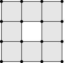
Figure 1: A regular CW-complex $S$ homotopy equivalent to the circle $\mathbb{S}^{1}$

We may be interested in studying the direct product $Y=S\times S\times S\times S$ which is naturally a regular CW-complex, homotopy equivalent to the $4$-torus, involving a total of $5308416=48^{4}$ cells. The fundamental group $\pi_{1}Y$ is free abelian on four generators $a,b,c,d$ and has a subgroup $H=\langle a^{5},b^{5},c^{5},d\rangle$ of index $125=5^{3}$. There is a corresponding $125$-fold covering map $p\colon\widetilde{Y}_{H}\rightarrow Y$. We may be interested in the integral homology groups $H_{n}(\widetilde{Y}_{H},\mathbb{Z})$. General theory tells us that $\widetilde{Y}_{H}$ is homeomorphic to $Y$, but if we were ignorant of this general fact then we might consider computing the homology $H_{n}(\widetilde{Y}_{H},\mathbb{Z})=H_{n}(C_{\ast}\widetilde{Y}_{H})$ directly from the cellular chain complex of $\widetilde{Y}_{H}$. The chain complex $C_{\ast}\widetilde{Y}_{H}$ of the 125-fold cover can we expressed in terms of the cellular chain complex $C_{\ast}\widetilde{Y}$ of the universal cover:

$$C_{\ast}\widetilde{Y}_{H}=C_{\ast}\widetilde{Y}\,\otimes_{\mathbb{Z}G}A$$ (2)

with $G=\pi_{1}Y$, $A=\mathbb{Z}G\,\otimes_{\mathbb{Z}H}\mathbb{Z}$. The desired homology $H_{n}(\widetilde{Y}_{H},\mathbb{Z})$ can be viewed as the homology $H_{n}(Y,A)$ of $Y$ with local coefficients in the module $A$. The chain complex $C_{\ast}\widetilde{Y}_{H}$ is a complex of free abelian groups of the following form.

$$\rightarrow 0\rightarrow\mathbb{Z}^{512000}\rightarrow\mathbb{Z}^{6144000}\rightarrow\mathbb{Z}^{31744000}\rightarrow\mathbb{Z}^{92160000}\rightarrow\mathbb{Z}^{164352000}\rightarrow \mathbb{Z}^{184320000}\rightarrow\mathbb{Z}^{126976000}\rightarrow\mathbb{Z}^{49152000}\rightarrow\mathbb{Z}^{8192000}$$ (3)

It is not practical to compute $H_{n}(\widetilde{Y}_{H},\mathbb{Z})$ by applying the Smith Normal Form algorithm directly to (3). An aim of this paper is to explain how simple homotopy equivalences, represented as discrete vector fields, can be used to produce a smaller homotopy equivalent chain complex from which the homology can be computed. An implementation of the techniques is available in the HAP package Ellis (November 2019) for the GAP system for computational algebra GAP (2013), and is illustrated in the computer code of in Table 1 which computes $H_{0}(\widetilde{Y}_{H},\mathbb{Z})=\mathbb{Z}$, $H_{1}(\widetilde{Y}_{H},\mathbb{Z})=\mathbb{Z}^{4}$, $H_{2}(\widetilde{Y}_{H},\mathbb{Z})=\mathbb{Z}^{6}$, $H_{3}(\widetilde{Y}_{H},\mathbb{Z})=\mathbb{Z}^{4}$, $H_{4}(\widetilde{Y}_{H},\mathbb{Z})=\mathbb{Z}$ from the regular CW-complex $Y=S\times S\times S\times S$.

gap> A:=[[1,1,1],[1,0,1],[1,1,1]];;
gap> S:=PureCubicalComplex(A);;
gap> S:=RegularCWComplex(S);;
gap> Y:=DirectProduct(S,S,S,S);
Regular CW-complex of dimension 8
gap> Size(Y);
5308416
gap> C:=ChainComplexOfUniversalCover(Y);
Equivariant chain complex of dimension 4
gap> G:=C!.group;;
[ f1, f2, f3, f4 ]
gap> H:=Group(G.1^5,G.2^5,G.3^5,G.4);
Group([ f1^5, f2^5, f3^5, f4 ])
gap> D:=TensorWithIntegersOverSubgroup(C,H);
Chain complex of length 4 in characteristic 0 .
gap> Homology(D,0);
[ 0 ]
gap> Homology(D,1);
[ 0, 0, 0, 0 ]
gap> Homology(D,2);
[ 0, 0, 0, 0, 0, 0 ]
gap> Homology(D,3);
[ 0, 0, 0, 0 ]
gap> Homology(D,4);
[ 0 ]

Table 1: Computing the homology of a 125-fold cover of a regular CW-complex $Y$ with 5308416 cells.

This computation involves a non-regular CW-complex $\widetilde{X}_{H}$ which is homotopy equivalent to $\widetilde{Y}_{H}$. More precisely, $\widetilde{X}_{H}$ is a finite cover of $X=S^{\prime\prime}\times S^{\prime\prime}\times S^{\prime\prime}\times S^{\prime\prime}$ with $S^{\prime\prime}$ the non-regular CW-complex of Figure 2 (right). The CW-complex $\widetilde{X}_{H}$ involves considerably fewer cells that $\widetilde{Y}_{H}$.

For some situations one may wish to work with a smaller regular CW-complex that is homeomorphic, and not just homotopy equivalent, to $\widetilde{Y}_{H}$. In the above example the number of cells in $\widetilde{Y}_{H}$ places its direct construction out of reach of computers with modest CPU and memory. But one could try to simplify the cell structure on $\widetilde{Y}_{H}$ so that it involves fewer cells. The obvious approach is to first simplify the cell structure on $Y$. In the above example we have $Y=S\times S\times S\times S$ with $S$ the CW-complex of Figure 1. We could replace $S$ by the homeomorphic regular CW-complex $S^{\prime}$ of Figure 2 (left) and then work with the space $Y^{\prime}=S^{\prime}\times S^{\prime}\times S^{\prime}\times S^{\prime}$ which is homeomorphic to $Y$.

                 

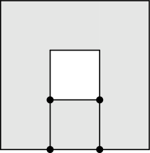
Figure 2: A regular CW-complex $S^{\prime}$ and a non-regular CW-complex $S^{\prime\prime}$.

Using an algorithm for simplifying the CW-structure on a regular CW-complex, the computer code in Table 2 illustrates the construction of the covering map $p\colon\widetilde{Y}^{\prime}_{H}\rightarrow Y^{\prime}$ which maps each cell of $\widetilde{Y}^{\prime}_{H}$ homeomorphically to a cell of $Y^{\prime}$.

gap> S:=SimplifiedComplex(S);
Regular CW-complex of dimension 2
gap> Size(S);
12
gap> Y:=DirectProduct(S,S,S,S);;
gap> U:=UniversalCover(Y);
Equivariant CW-complex of dimension 8
gap> G:=U!.group;;
gap> H:=Group(G.1^5,G.2^5,G.3^5,G.4);;
gap> p:=EquivariantCWComplexToRegularCWMap(U,H);
Map of regular CW-complexes
gap> UH:=Source(p);
Regular CW-complex of dimension 8
gap> Size(UH);
2592000

Table 2: Computing a 125-fold covering map $p\colon\widetilde{Y}^{\prime}_{H}\twoheadrightarrow Y^{\prime}$ with $Y^{\prime}$ homeomorphic to a regular CW-complex with 5308416 cells.

The data types, algorithms, and mathematical theory underlying the above example computations are explained in Sections 4 and 6.

4 Computing chains on the universal cover

Let $Y$ be a connected regular CW-complex with only finitely many cells. One algorithm for constructing a finite presentation for the fundamental group $G=\pi_{1}Y$ was described in Brendel et al. (2015), Ellis (2019), details of which are recalled below. It is well-known that, in general, there is no algorithm for solving the word problem in the finitely presented group $G$. But this unsolvability of the word problem is not relevant to our goals. Let $\widetilde{Y}$ be the universal cover of $Y$ with canonical CW-structure inherited from $Y$. The cellular chain group $C_{n}\widetilde{Y}$ is a free $\mathbb{Z}G$-module whose free generators correspond to the $n$-cells of $Y$. The module $C_{n}\widetilde{Y}$ can be represented on a computer by specifying the number ${\rm rank}_{\mathbb{Z}G}(C_{n}\widetilde{Y})$ of free generators and specifying the free presentation for $G$. We denote by $e^{n}_{i}$ an $n$-cell of $Y$, and we denote by $\tilde{e}^{n}_{i}$ some preferred lift of $e^{n}_{i}$ in $\widetilde{Y}$. For $g\in G$ we denote by $g\tilde{e}^{n}_{i}$ the n-cell obtained by applying the action of $g$ to $\tilde{e}^{n}_{i}$. We also use $\tilde{e}^{n}_{i}$ to denote a free generator of the $\mathbb{Z}G$-module $C_{n}\widetilde{Y}$. The boundary homomorphism $\partial_{n}\colon C_{n}\widetilde{Y}\rightarrow C_{n-1}\widetilde{Y}$ is $G$-equivariant and can be represented by specifying $\partial_{n}(\tilde{e}^{n}_{i})$ for each free generator of $C_{n}\widetilde{Y}$. We now describe how an explicit expression for $\partial_{n}(\tilde{e}^{n}_{i})$ can be computed using induction on $n$.

We view the $1$-skeleton $Y^{1}$ as a graph. Let $T$ denote some fixed choice of maximal tree in $Y^{1}$. The tree $T$ has the same vertices as $Y^{1}$ but, typically, fewer edges. Each edge $e$ in $Y^{1}$ admits two possible orientations; let us arbitrarily fix one choice of orientation for each edge. An oriented edge $e$ in $Y^{1}\setminus T$ determines an oriented circuit in $Y^{1}$ whose image consists of the oriented edge $e$ and some oriented edges from $T$. We denote this oriented circuit by $\omega(e)$. The association $e\mapsto\omega(e)$ induces a function $\omega\colon\{{\rm edges\ in\ }Y^{1}\setminus T\}\longrightarrow G$. This function extends to a function $\omega\colon\{{\rm edges\ in\ }Y^{1}\}\longrightarrow G$ which sends oriented edges in $T$ to the trivial element of the fundamental group.

Let $F$ denote the free group on the symbols $\omega(e)$ where $e$ runs over the edges in $Y^{1}\setminus T$. Each $2$-cell $e^{2}$ in $Y^{2}$ admits two possible orientations; let us arbitrarily fix one choice of orientation for each $2$-cell. The boundary of an oriented $2$-cell then spells a word in $F$ that represents the trivial word in the fundamental group $G$. It is well-known Hatcher (2002), Spanier (1981) that $G$ admits a free presentation with one generator $\omega(e)$ for each edge $e\subset Y^{1}\setminus T$, and one relator for each $2$-cell in $Y$.

Let us now consider how to compute an expression for the boundary $\partial_{n}(\tilde{e}^{n}_{i})$ of each free generator of the $\mathbb{Z}G$-module $C_{n}(\widetilde{Y})$. We first consider the case $n=1$. The $1$-cell $\tilde{e}^{1}_{i}$ in $\widetilde{Y}$ maps to the $1$-cell $e^{1}_{i}$ in $Y$. Suppose that $e^{0}_{j},e^{0}_{k}$ are the two boundary vertices of $e^{1}_{i}$, and that the orientation of $e^{1}_{i}$ corresponds to a direction which starts at $e^{0}_{j}$ and ends at $e^{0}_{k}$. Suppose also that in the cellular chain complex, which involves choices of orientation, the boundary homomorphism satisfies

$$\partial_{1}(e^{1}_{i})=e^{0}_{k}-e^{0}_{j}\ .$$ (4)

Then we set

$$\partial_{1}(\tilde{e}^{1}_{i})=g\tilde{e}^{0}_{k}-\tilde{e}^{0}_{j}\ ,\ \ \ {\rm where\ }g=\omega(e^{1}_{i}).$$ (5)

Suppose now that we have computed $\partial_{1}(\tilde{e}^{1}_{i})$, $\partial_{2}(\tilde{e}^{2}_{i})$, …, $\partial_{n}(\tilde{e}^{n}_{i})$ for all free generators in degrees $\leq n$. To compute $\partial_{n+1}(\tilde{e}^{n+1}_{i})$ we first compute

$$\partial_{n+1}e^{n+1}_{i}=\epsilon_{1}e^{n}_{i_{1}}+\epsilon_{2}e^{n}_{i_{2}}+\cdots+\epsilon_{m}e^{n}_{i_{m}}$$ (6)

with $\epsilon_{i}=\pm 1$. Having computed (6) it remains to determine representatives of group elements $g_{i_{1}},\ldots,g_{i_{m}}$ in the finitely presented group $G$ such that the element

$$\partial_{n+1}\tilde{e}^{n+1}_{i}=\epsilon_{1}g_{i_{1}}\tilde{e}^{n}_{i_{1}}+\epsilon_{2}g_{i_{2}}\tilde{e}^{n}_{i_{2}}+\cdots+\epsilon_{m}g_{i_{m}}\tilde{e}^{n}_{i_{m}}$$ (7)

satisfies $\partial_{n}(\partial_{n+1}\tilde{e}^{n+1}_{i})=0$. We set $g_{i_{1}}=1\in G$. Suppose $\partial(g_{i_{1}}\tilde{e}^{n}_{i_{1}})$ contains $\pm h\tilde{e}^{n-1}_{j}$ as a summand, some $h\in G$. Then for some $i_{j}\neq i_{1}$ the boundary $\partial(\tilde{e}^{n}_{i_{j}})$ must contain $\mp h^{\prime}\tilde{e}^{n-1}_{j}$ as a summand for some $h^{\prime}\in G$. In (7) we set $g_{i_{j}}=hh^{\prime-1}$. We continue with this method of matching summands in the boundaries $\partial\tilde{e}^{n}_{i_{k}}$ in order to determine all the $g_{i_{k}}$ in (7). Note that the method does not require a solution to the word problem in the finitely generated group $G$.

Suppose given a finitely generated abelian group $A$ and group homomorphism $\phi\colon G\rightarrow Aut(A)$ specified on generators of $G$. This data constitutes a $\mathbb{Z}G$-module $A$. Starting from our computer representation of the chain complex $C_{\ast}\widetilde{Y}$, it is routine to implement the cochain complex ${\rm Hom}_{\mathbb{Z}G}(C_{\ast}\widetilde{Y},A)$ of finitely generated abelian groups, and also the chain complex $C_{\ast}\widetilde{Y}\otimes_{\mathbb{Z}G}A$. In particular, given a finite set of elements in $G$ that generates a finite index subgroup $H<G$, we can use coset enumeration to construct the $\mathbb{Z}G$-module $A=\mathbb{Z}G\otimes_{\mathbb{Z}H}\mathbb{Z}$; in this case the chain complex $C_{\ast}\widetilde{Y}\otimes_{\mathbb{Z}G}A$ can be viewed as the chain complex $C_{\ast}\widetilde{Y}_{H}$ of the finite covering space $p\colon\widetilde{Y}_{H}\twoheadrightarrow Y$ with $p$ inducing an isomorphism $\pi_{1}\widetilde{Y}_{H}\cong H$. Since $\widetilde{Y}_{H}$ is a regular CW-complex, its CW-structure (i.e. its face lattice) is completely determined by the chain complex $C_{\ast}\widetilde{Y}_{H}$. Thus, in principle, we have an algorithm for computing the finite cover $\widetilde{Y}_{H}$. Furthermore, in principle, the Smith Normal Form algorithm can be used to compute the local cohomology $H^{n}(Y,A)$ and homology $H_{n}(Y,A)$ for any $\mathbb{Z}G$-module $A$ which is finitely generated over $\mathbb{Z}$.

However, for practical computations, such as those in Tables 1 and 2, there are two issues with the above theoretical algorithm. Firstly, if the above method is applied directly then the finitely presented fundamental group $G=\pi_{1}Y$ will typically involve excessive numbers of generators and relators. These numbers need to be reduced in a way that retains the relationship between the finite presentation and the cellular structure of $Y$ if, for instance, one wants to apply coset enumeration and the Reidemeister-Schreier algorithm to list free presentations of subgroups $H\leq G$ of given index $k$ in order to enumerate all $k$-fold covers of $Y$. Table 3 provides a computation in which such an enumeration is needed. Secondly, the number of cells in $Y$ will typically be large, and consequently the number of generators of the chain groups $C_{n}\widetilde{Y}\otimes_{\mathbb{Z}G}A$ will typically make it impractical to apply the Smith Normal Form algorithm directly to the chain complex $C_{\ast}\widetilde{Y}\otimes_{\mathbb{Z}G}A$ or cochain complex ${\rm Hom}_{\mathbb{Z}G}(C_{\ast}\widetilde{Y},A)$. We need a method for reducing the number of cells in $Y$ and $\widetilde{Y}$ in a way that retains the homotopy types of $Y$ and $\widetilde{Y}$ or even, for some purposes, their homeomorphism types. The code in Table 1 reduces the number of cells while retaining only the homotopy type of $Y$. The code in Table 2 retains the homeomorphism type of $Y$. We now describe our approach to addressing these practical issues.

Let us first recall from Ellis (2019) a simple method aimed at reducing the number of cells in a regular CW-complex $Y$ while retaining the homeomorphism type of $Y$. The simplification procedure invoked in the computer code of Table 2 is based on the observation that if a regular CW-complex $Y$ contains a $k$-cell $e^{k}$ lying in the boundary of precisely two $(k+1)$-cells $e^{k+1}_{1},e^{k+1}_{2}$ with identical coboundaries then these three cells can be removed and replaced by a single cell of dimension $k+1$. The topological space $Y$ is unchanged; only its CW-structure changes. The resulting CW-structure will not in general be regular. However, it will be regular if the sets $V_{0},V_{1},V_{2}$ of cells lying in the boundaries of $e^{k},e^{k+1}_{1},e^{k+1}_{2}$ respectively are such that $V_{1}\cap V_{2}=V_{0}\cup\{e^{k}\}$. The result of this kind of simplification procedure is illustrated in Figure 3.

                     

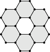
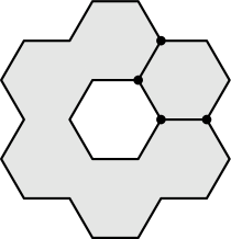
Figure 3: Regular CW-complex before and after simplification.

The procedure is formalized as Algorithm 4.1.

Algorithm 4.1 Simplification of a regular CW-structure.

1:A regular CW-complex $Y$.

2:A regular CW-complex $X$ with $Size(X)\leq Size(Y)$ and with $|X|$ homeomorphic to $|Y|$.

3:procedure 

4:     Let $X$ be a copy of $Y$.

5:     while there exists a cell $e^{k}$ in $X$ with precisely two cells $e^{k+1}_{1},e^{k+1}_{2}$ in its coboundary and these two cells have identical coboundaries do

6:         Compute the sets $V_{0}$, $V_{1}$, $V_{2}$ of cells in the boundaries of $e^{k}$, $e^{k+1}_{1}$, $e^{k+1}_{2}$.

7:         if $|V_{1}\cap V_{2}|=1+|V_{0}|$ then

8:              Remove the cells $e^{k}$, $e^{k+1}_{1}$, $e^{k+1}_{2}$ from $X$ and add a new $(k+1)$-cell $f^{k+1}$ to $X$ whose boundary is the union of the boundaries of $e^{k+1}_{1}$ and $e^{k+1}_{2}$ minus the cell $e^{k}$. Adjust coboundaries accordingly.

9:         end if

10:     end while

11:     Return $X$.

12:end procedure

It can be useful, for instance, in the study of the homeomorphism type of $CW$-complexes $Y$ arising as knot complements in $\mathbb{R}^{3}$, especially when $Y$ is constructed from experimental data, such as knotted proteins, with natural CW-structure involving a vast number of cells (see Brendel et al. (2015)).

We now turn to a method for reducing the number of cells in $Y$ in a way that retains only the homotopy type of $Y$. For this we first recall the following notion.

Definition 4.1.

A discrete vector field on a regular CW-complex $Y$ is a collection of pairs $(s,t)$, which we call arrows and denote by $s\rightarrow t$, satisfying

1. $s,t$ are cells of $X$ with $\dim(t)=\dim(s)+1$ and with $s$ lying in the boundary of $t$. We say that $s$ and $t$ are involved in the arrow, that $s$ is the source of the arrow, and that $t$ is the target of the arrow.

2. any cell is involved in at most one arrow.

The term discrete vector field is due to Forman (1998). In an earlier work Jones (1988) Jones calls this concept a marking.

A discrete vector field is said to be finite if it consists of just finitely many arrows. By a chain in a discrete vector field we mean a sequence of arrows

$$\ldots,s_{1}\rightarrow t_{1},s_{2}\rightarrow t_{2},s_{3}\rightarrow t_{3},\ldots$$

where $s_{i+1}$ lies in the boundary of $t_{i}$ for each $i$. A chain is a circuit if it is of finite length with source $s_{1}$ of the initial arrow $s_{1}\rightarrow t_{1}$ lying in the boundary of the target $t_{n}$ of the final arrow $s_{n}\rightarrow t_{n}$. A discrete vector field is said to be admissible if it contains no circuits and no chains that extend infinitely to the right. When the CW-complex $Y$ is finite a discrete vector field is admissible if it contains no circuits. We say that an admissible discrete vector field is maximal if it is not possible to add an arrow while retaining admissibility. A cell in $X$ is said to be critical if it is not involved in any arrow.

Theorem 2.

Forman (2002, 1998) If $Y$ is a regular CW-complex with admissible discrete vector field then there is a homotopy equivalence

$$Y\simeq X$$

where $X$ is a CW-complex whose cells are in one-one correspondence with the critical cells of $X$.

An arrow on $Y$ can be viewed as representing a simple homotopy, as introduced in Whitehead (1950). The theorem just says that an admissible discrete vector field represents some sequence of (in some sense ’composable’) simple homotopies starting at $Y$ and ending at $X$.

There are various algorithms for constructing an admissible discrete vector field on a finite regular CW-complex $Y$. The algorithm implemented in the HAP package is Algorithm 4.2, which we recall from Ellis and Hegarty (2014), Ellis (2019).

Algorithm 4.2 Discrete vector field on a regular CW-complex.

1:A finite regular CW-complex $Y$

2:A maximal admissible discrete vector field on $Y$.

3:procedure 

4:     Partially order the cells of $Y$ in any fashion.

5:     At any stage of the algorithm each cell will have precisely one of the following three states: (i) critical, (ii) potentially critical, (iii) non-critical.

6:     Initially deem all cells of $Y$ to be potentially critical.

7:     while there exists a potentially critical cell do

8:         while there exists a pair of potentially critical cells $s,t$ such that: $\dim(t)=\dim(s)+1$; $s$ lies in the boundary of $t$; no other potentially critical cell of dimension $\dim(s)$ lies in the boundary of $t$; do

9:              Choose such a pair $(s,t)$ with $s$ minimal in the given partial ordering.

10:              Add the arrow $s\rightarrow t$ and deem $s$ and $t$ to be non-critical.

11:         end while

12:         if there exists a potentially critical cell then

13:              Choose a minimal potentially critical cell and deem it to be critical.

14:         end if

15:     end while

16:end procedure

In line 2 of the algorithm the cells could be partially ordered in some way that ensures any cell of dimension $k$ is less than all cells of dimension $k+1$. This partial ordering guarantees that the resulting discrete vector field on a path-connected regular CW-complex $Y$ will have a unique critical $0$-cell.

A CW-complex $X$ is said to be reduced if it has only one cell in dimension $0$. There is a standard correspondence between the $2$-skeleton of such a space and a presentation of its fundamental group $G=\pi_{1}X$. This correspondence together with Theorem 2 and Algorithm 4.2 constitute our algorithm for finding a presentation for the fundamental group of any connected CW-complex $Y$. The presentation has one generator for each critical $1$-cell of $Y$ and one relator for each critical $2$-cell. Each oriented critical $2$-cell $e\subset Y$ determines an oriented circuit $\omega(e)$ in $Y^{1}$; the discrete vector field provides a deformation of this circuit $\omega(e)$ into a circuit $\omega^{\prime}(e)$ each of whose oriented edges $t$ is either critical or else the target of some arrow $s\rightarrow t$ with $s$ a $0$-cell. The subsequence of $\omega^{\prime}(e)$ consisting of the oriented critical edges spell a word in the free group on the generators of the presentation. For illustrations and further details of this algorithm see Brendel et al. (2015), Ellis (2019).

Let us now address the question of how to reduce the number of cells in the universal cover $\widetilde{Y}$ of a connected regular CW-complex in a way that retains its homotopy type. It suffices to note that any discrete vector field on $Y$ induces a discrete vector field on $\widetilde{Y}$: there is an arrow $\tilde{s}\rightarrow\tilde{t}$ on $\widetilde{Y}$ if and only if if $s\rightarrow t$ is an arrow on $Y$ where $\tilde{s},\tilde{t}$ are cells in the universal cover that map to $s,t$ , and where $\tilde{s}$ lies in the boundary of $\tilde{t}$. Furthermore, if the discrete vector field on $Y$ is admissible then so too is the induced vector field. Let $X\simeq Y$ be the homotopy equivalence of Theorem 2. This equivalence induces a homotopy equivalence of universal covers $\widetilde{X}\simeq\widetilde{Y}$ and a chain homotopy equivalence of cellular chain complexes $C_{\ast}\widetilde{X}\simeq C_{\ast}\widetilde{Y}$. The cells in $\widetilde{X}$ are in one-one correspondence with the critical cells in the induced discrete vector field on $\widetilde{Y}$. The cellular chain complex $C_{\ast}\widetilde{X}$ on the (typically non-regular) CW-complex $X$ is readily constructed directly from the cell structure and admissible discrete vector field of $Y$. This construction is implemented in HAP as the function ChainComplexOfUniversalCover(Y) which inputs $Y$, constructs a maximal discrete vector field on $Y$, uses this vector field to compute a presentation for $\pi_{1}Y\cong\pi_{1}X$, and finally returns the $\pi_{1}Y$-equivariant chain complex $C_{\ast}(\widetilde{X})$.

5 From diagrams to CW-complexes

Suppose that $N$ is a compact topological submanifold of $\mathbb{R}^{n+2}$ with $n=1$ or $2$, and that $p\colon\mathbb{R}^{n+2}\twoheadrightarrow\mathbb{R}^{n+1}$ is a projection onto a hyperplane. Let $M\subset\mathbb{R}^{n+2}$ denote a submanifold homeomorphic to the closed unit disk, whose interior $\mathring{M}$ contains $N$. Set $D^{n+1}=p(M)$. We say that the pair $p(N)\subset D^{n+1}$ is a diagram for $N$. Under fairly general conditions it is possible to embellish the diagram with information on the preimage $p^{-1}(y)$ of certain points $y\in N$ so that the ambient isotopy type of the embedding $N\hookrightarrow\mathbb{R}^{n+1}$ can be recovered from the embellishment. We are then interested in using the embellished diagram to construct a regular CW-structure on $M$ containing a CW-subspace ambient isotopic to $N$. We illustrate the idea with several examples.

5.1 A closed $1$-manifold $N$ in $\mathbb{R}^{3}$.

As an illustration let us consider the trefoil knot whose embedding $\kappa\colon\mathbb{S}^{1}\hookrightarrow\mathbb{R}^{3}$ is illustrated in Figure 4 (left). We set $N$ equal to the image of $\kappa$.

           

Figure 4: Trefoil knot.

A diagram $(D^{2},p(N))$ for the trefoil is shown in Figure 4 (middle). A CW-structure on $D^{2}$ is shown in Figure 4 (right). The CW-structure is designed to reflect the under crossing/over crossing structure of the knot projection. Let the unit interval $[0,1]$ be given a CW-structure involving two $0$-cells and one $1$-cell. The

Figure 5: CW-subcomplex of $M$ ambient isotopic to the Trefoil knot.

CW-complex formed by adjoining a $2$-cell and $3$-cell to each end of the cylinder $D^{2}\times[0,1]$ is homeomorphic to a $3$-ball $M$ and contains, in its interior, a CW-subcomplex $N$ ambient isotopic to the trefoil knot (see Figure 5). The construction of this CW-structure on the trefoil embedding readily extends to an algorithm which inputs a symbolic representation of a knot or link and returns a CW-decomposition of a $3$-ball $M$ containing the knot or link as a subcomplex of the $1$-skeleton.

We are interested in studying the complement $M\setminus N$. However, the difference of CW-complexes is not a CW-complex. This technicality can be overcome by constructing a small open tubular neighbourhood $N_{\epsilon}$ of $N$ and extending the cell structure on $M\setminus N$ to a CW-structure on $M\setminus N_{\epsilon}$. Details of the construction are given in Section 10.

5.2 A $3$-manifold $N$ in $\mathbb{R}^{3}$, and the complement of its interior.

There are a number of succinct symbolic representations of links in $\mathbb{R}^{3}$. One representation is based on arc diagrams of links such as the arc diagram for the trefoil shown in Figure 6 (left).

         

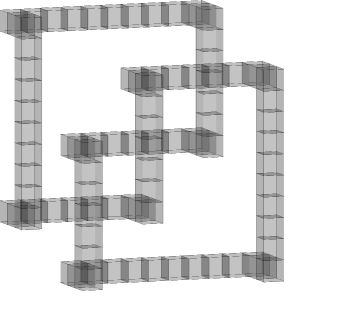
Figure 6: Arc diagram for the trefoil knot (left) and corresponding pure cubical complex (right).

An arc diagram is a planar link diagram involving only horizontal and vertical straight lines, with vertical lines always passing over the horizontal lines. An arc diagram can be represented symbolically by a suitable ordered list $\ell$ of ordered pairs of positive integers. The list $\ell=[[2,5],[1,3],[2,4],[3,5],[1,4]]$ represents the arc diagram of Figure 6. The $i$th pair in the list specifies the starting column and end column of the $i$th horizontal line, where the bottom line is the $1$st horizontal line, and the leftmost column is the $1$st column.

An arc diagram leads to a very natural, though somewhat inefficient, representation of the corresponding link as a $3$-dimensional CW-manifold $N$ with boundary. To explain how, we endow $\mathbb{R}^{n}$ with the regular CW-structure in which each $n$-cell has closure equal to a unit cube with standard CW-structure and with centre an integer vector $c\in\mathbb{Z}^{n}$. A finite CW-subcomplex of $\mathbb{R}^{n}$ is said to be an $n$-dimensional cubical complex. Such a complex is said to be pure if each cell lies in the closure of some $n$-cell. An arc presentation for $N$ gives rise in a fairly obvious fashion to a diagram $(D^{2},p(N))$ with $D^{2}$ a $2$-dimensional pure cubical complex homeomorphic to a disk. Now let the real interval $[0,5]$ be given a CW-structure with integers the $0$-cells. The desired $3$-dimensional pure cubical complex $N$ is realized as a CW-subcomplex of the direct product $D^{2}\times[0,5]$.

The $3$-dimensional pure cubical complex $N_{\ell}$ corresponding to the example list for the trefoil is shown in Figure 6 (right). Let $M$ denote a contractible pure cubical complex in $\mathbb{R}^{3}$ whose interior contains $N_{\ell}$. Then the complement $X=M\setminus\mathring{N_{\ell}}$ is a pure cubical complex homotopy equivalent to the complement $\mathbb{R}^{3}\setminus N_{\ell}$. The construction of the CW-complex $X$ is implemented in HAP, with $M$ chosen to be a minimal solid rectangular pure cubical complex whose interior contains $N_{\ell}$. For the trefoil knot of Figure 6 (right) the implemented CW-complex $X$ contains 13291 cells.

5.3 A more efficient complement of the interior of a $3$-manifold $N$ in $\mathbb{R}^{3}$.

Pure cubical complexes are particularly useful as a tool for converting a range of experimental data into regular CW-complexes in order to analyse underlying topological features (see for instance Ellis (2019)). However, the resulting CW-complexes tend to be large and cumbersome to work with on a computer. From the viewpoint of theoretical knot theory, one would like algorithms for converting a symbolic description of a link or knotted surface complement into a regular CW-complex with relatively few cells so that computations of fundamental groups and local cohomology run efficiently. We now explain, in four steps, how to construct a smaller CW-structure on the complement $Y_{\ell}=M\setminus\mathring{N_{\ell}}$ of a link $N_{\ell}$ arising from an arc presentation $\ell$.

Step 1. Let us suppose that the arc diagram for the list $\ell$ involves precisely $h$ horizontal lines and precisely $k$ crossings. Let $D^{2}_{\ell}$ denote the unit $2$-disk with $2h$ non-overlapping subdisks removed. The arc diagram for $\ell$ then determines a (nearly) canonical CW structure on $D^{2}_{\ell}$. This is illustrated in Figure 7 for the trefoil. (The CW structure could be made canonical by, for instance, insisting that the two $0$-cells on the boundary of the disk be connected to the bottom left-most and top right-most vertices of the inner diagram.)

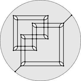
Figure 7: CW-structure on a $2$-dimensional disk $D^{2}_{\ell}$ with ten holes.

In general the CW structure has $V=4h+4k+2$ vertices, $E=8h+8k+4$ edges, and $E-V-2h+1$ cells of dimension $2$. The formula for the number of $2$-cells is derived from the Euler characteristic $\chi(D^{2}_{\ell})=1-2h$. The space $D^{2}_{\ell}$ has a total of $14h+16k+9$ cells.

Step 2. Let $\mathbb{I}$ denote the unit interval with $CW$-structure involving two vertices and one edge. Now form the direct product $D^{2}_{\ell}\times\mathbb{I}$. This is a CW-complex which we view as a solid cylinder from which $2h$ vertical tubes, running from bottom to top, have been removed. It involves a total of $3(14h+16k+9)$ cells.

Step 3. Corresponding to each horizontal line in the arc diagram glue one $2$-cell to the bottom of $D^{2}_{\ell}\times\mathbb{I}$, and corresponding to each vertical line in the arc diagram glue one $2$-cell to the top of $D^{2}_{\ell}\times\mathbb{I}$. More precisely, these $2h$ $2$-cells are glued so that the resulting CW-complex $W_{\ell}=D^{2}_{\ell}\times\mathbb{I}\cup\bigcup_{i-1}^{2h}e^{2}$ is homotopy equivalent to the link complement $\mathbb{R}^{3}\setminus M_{\ell}$.

Step 4. Glue one $3$-cell and one $2$-cell to the bottom of $W_{\ell}$, and glue one $3$-cell and one $2$-cell to the top of $W_{\ell}$ in a way that the resulting CW-complex $Y_{\ell}=W_{\ell}\cup\bigcup_{i=1}^{2}e^{2}\cup\bigcup_{i=1}^{2}e^{3}$ is homeomorphic to $M\setminus\mathring{N}_{\ell}$. The CW-complex $Y_{\ell}$ involves a total of $3(14h+16k+9)+2h+4$ cells.

5.4 A closed $2$-manifold $N$ in $\mathbb{R}^{4}$.

In order to specify an embedding $N\hookrightarrow\mathbb{R}^{4}$ of a closed surface $N$ we can start by specifying a diagram $(D^{3},p(N))$ with $D^{3}$ a regular CW-complex homeomorphic to a closed $3$-ball, and with $p(N)\subset D^{3}$ a CW-subcomplex lying in the interior of $D^{3}$. The CW-subcomplex $p(N)$ need not be a surface; we allow it to have singular points $y\in p(N)$ for which there exists no open set of $p(N)$ containing $y$ and homeomorphic to an open $2$-disk. But we do require the collection of singular points to be either empty or to form a closed $1$-manifold. For instance, in the usual projection of the Klein bottle into $\mathbb{R}^{3}$ the singular points form a circle (see Figure 8).

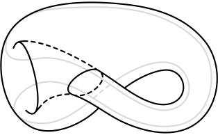
Figure 8: Klein bottle

We say that the CW-complex $p(N)$ is a self-intersecting surface. To complete the specification of the embedding of the surface $N$ we set $M=D^{3}\times[0,k]$ where $k$ is a positive integer and the interval is given a CW-structure with $0$-cells the integers. Let $p\colon M\twoheadrightarrow D^{3}$ be the projection. To specify a CW-manifold $N\subset M$ we just need to specify, in some fashion, the cells in the preimage $p^{-1}(e)$ for each cell $e\subset p(N)$.

The discussion in Subsection 5.3 can be interpreted as a method for representing an embedding of one or more tori into $\mathbb{R}^{3}$ by means of an arc presentation. This representation is readily extended to one for self-intersecting tori whose singular points form a $1$-manifold.

Given an embedding of a closed surface $N$ into $\mathbb{R}^{4}$, we can then construct a small open tubular neighbourhood $N_{\epsilon}$ of $N$ and extend the cell structure on $M\setminus N$ to a CW-structure on $M\setminus N_{\epsilon}$. Details of the neighbourhood construction are given in Section 10.

6 Some data types

For completeness, we recall from Ellis (2019) the main data types used in implementing the above discussion.

Data type 6.1.

A regular CW-complex $X$ is represented as a component object X with the following components:

• X!.boundaries[n+1][k] is a list of integers $[t,a_{1},...,a_{t}]$ recording that the $a_{i}$th cell of dimension $n-1$ lies in the boundary of the $k$th cell of dimension $n$.

• X!.coboundaries[n][k] is a list of integers $[t,a_{1},...,a_{t}]$ recording that the $k$th cell of dimension $n$ lies in the boundary of the $a_{i}$th cell of dimension $n+1$.

• X!.nrCells(n) is a function returning the number of cells in dimension $n$.

• X!.properties is a list of properties of the complex, each property stored as a pair such as $[``dimension",4]$.

Data type 6.2.

A discrete vector field on a regular CW-complex is represented as a regular CW-complex X with the following additional components, each of which is a $2$-dimensional array:

• X!.vectorField[n][k] is equal to the integer $k^{\prime}$ if there is an arrow from the $k$th cell of dimension $n-1$ to the $k^{\prime}$th cell of dimension $n$. Otherwise X!.vectorField[n][k] is unbound.

• X!.inverseVectorField[n][k’] is equal to the integer $k$ if there is an arrow from the $k$th cell of dimension $n-1$ to the $k^{\prime}$th cell of dimension $n$. Otherwise X!.inverseVectorField[n][k’] is unbound.

Data type 6.3.

A $G$-CW-complex $Y$ with regular CW-structure is represented by a component object Y which consists of the following components:

• Y!.group is a group $G$. (This can be stored in one of several possible formats including: finitely presented group; matrix group; power-commutator presented group; finite permutation group … .)

• Y!.elts is a list of some of the elements of $G$.

• Y!.dimension(n) is a function that returns a non-negative integer equal to the number of distinct $G$-orbits of $n$-dimensional cells in the $G$-equivariant CW-complex $|Y|$ modelled by the data type. We let $e^{n}_{k}$ denote a fixed representative of the $k$th orbit of $n$-dimensional cells.

• Y!.stabilizer(n,k) returns the subgroup of $G$ consisting of those elements $\phi\in G$ that map $e^{n}_{k}$ homeomorphically to itself.

• Y!.boundary(n,k) returns a list $[[i_{1},g_{1}],\ldots,[i_{m},g_{m}]]$ where each term $[i,g]$ is a pair of non-zero integers with $g$ positive. A pair $[i,g]$ records that $\phi_{g}(e^{n-1}_{|i|})$ lies in the boundary of $e^{n}_{k}$, where $\phi_{g}$ is the $g$th term of the list Y!.elts. (The sign of $i$ plays a role when we consider homology.)

• Y!.properties is a list of properties of the space, each property stored as a pair such as $[``dimension",4]$.

Data type 6.4.

A chain complex $C_{\ast}$ of finitely generated free modules over $\mathbb{Z}$ is represented as a component object C with the following components:

• C!.dimension(k) is a function which returns the rank of the module $C_{k}$.

• C!.boundary(k,j) is a function which returns the image in $C_{k-1}$ of the $j$th free generator of $C_{k}$. Elements in $C_{k-1}$ are represented as vectors (i.e. lists) over $\mathbb{Z}$ of length equal to the rank of $C_{k-1}$.

• C!.properties is a list of properties of the complex, each property stored as a pair such as $[``length",4]$.

7 The spun Hopf link and the tube of the welded Hopf link

We now give a computer proof of a variant on Theorem 10 in Kauffman and Faria Martins (2008). We opt to work in the inefficient category of pure cubical complexes as a means of demonstrating that computations are practical even when CW-complexes involve large numbers of cells.

Figure 9 shows a $3$-dimensional pure cubical complex $Y$ formed from the union of two intersecting pure cubical subcomplexes each of which is homotopy equivalent to a torus. The space $Y$ is a union of 1632 cubical $3$-cubes. The four horizontal rectangular tubes of $Y$ have a $3\times 3$ cross section. The four vertical rectangular tubes of $Y$ have a $7\times 7$ cross section.

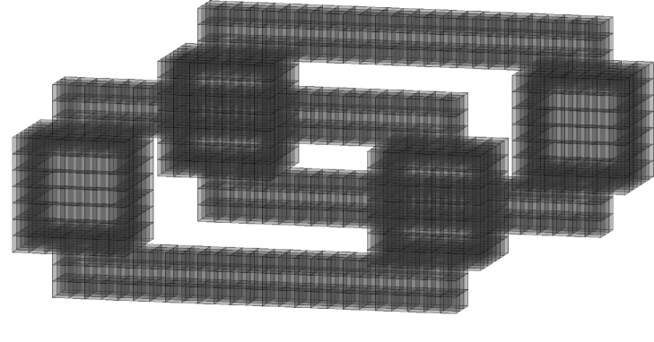
Figure 9: Union of two $3$-dimensional pure cubical complexes, each homotopy equivalent to a torus.

The central axes of the horizontal tubes and vertical tubes lie in a common plane. We use $Y$ to construct two $4$-dimensional pure cubical complexes $S$ and $T$ as follows.

To construct $S$ we first assign integers $t$, called temperature, to each $3$-cube of $Y$. To most $3$-cubes we assign a single temperature $t$, but a few $3$-cubes are assigned three temperatures. All $3$-cubes in the top and bottom horizontal rectangular tubes are assigned one temperature $t=0$. All $3$-cubes in the four vertical rectangular tubes are again assigned the one temperature $t=0$. The middle two horizontal rectangular tubes each have length 25. In these two tubes the $x$-coordinate of a cube’s centre determines its temperature(s) according to the profiles shown in Figure 10. Profile 1 is the cross sectional temperature profile of the upper-middle horizontal tube of $Y$; the lower-middle horizontal tube of $Y$ is assigned Profile 2. The space $S$ is the $4$-dimensional pure cubical complex whose $4$-cubes are centred on the integer vectors $(x,y,z,t)$ where $(x,y,z)$ is the centre of a $3$-cube of $Y$ with temperature $t$. The space $S$ is homotopy equivalent to a disjoint union of two tori.

The space $T$ is a $4$-dimensional pure cubical complex constructed in the same fashion as $S$ except that the temperature profiles of Figure 11 are used in place of those of Figure 10. The space $T$ is also homotopy equivalent to a disjoint union of two tori.

Profile 1:

Profile 2:

Figure 10: Profiles of cube temperatures for $S$

Profile 1:

Profile 2:

Figure 11: Profiles of cube temperatures for $T$

Let $\mathring{S}$ and $\mathring{T}$ denote the interiors of $S$ and $T$. The complements $\mathbb{R}^{4}\setminus\mathring{S}$ and $\mathbb{R}^{4}\setminus\mathring{T}$ are subcomplexes of the CW-complex $\mathbb{R}^{4}$, both involving infinitely many cells. It is straightforward to construct finite deformation retracts $X_{S}\subset\mathbb{R}^{4}\setminus\mathring{S}$ and $X_{T}\subset\mathbb{R}^{4}\setminus\mathring{T}$ where $X_{S}$ and $X_{T}$ are $4$-dimensional pure cubical complexes. The computer code of Table 3 computes a CW-complex $X_{T}$ involving 4508573 cells, together with a sorted list $Inv(X_{T})$ of all possible abelian invariants of the second homology groups $H_{2}(\widetilde{X}_{H},\mathbb{Z})$ of 5-fold covering spaces $X_{H}$ for $X_{T}$. The list $Inv(X_{T})$ is an invariant of the homotopy type of $X_{T}$, and establishes that there are $5$-fold covers with $H_{2}(\widetilde{X}_{H},\mathbb{Z})=\mathbb{Z}^{12}$ and $5$-fold covers with $H_{2}(\widetilde{X}_{H},\mathbb{Z})=\mathbb{Z}^{16}$.

gap> T:=HopfSatohSurface();;
gap> XT:=PureComplexComplement(T);;
gap> XT:=RegularCWComplex(XT);
Regular CW-complex of dimension 4
gap> Size(XT);
4508573

gap> C:=ChainComplexOfUniversalCover(XT);;
gap> L:=Filtered(LowIndexSubgroups(C!.group,5), g->Index(C!.group,g)=5);;
gap> invXT:=List(L,g->Homology(TensorWithIntegersOverSubgroup(C,g),2));;
gap> invXT:=SSortedList(invXT);
[ [ 0, 0, 0, 0, 0, 0, 0, 0, 0, 0, 0, 0 ],
  [ 0, 0, 0, 0, 0, 0, 0, 0, 0, 0, 0, 0, 0, 0, 0, 0 ] ]

Table 3: Computing the CW-complex $X_{T}$ and an invariant of its homotopy type.

Similar commands can be applied to $X_{S}$ to find that for all $5$-fold covers $X_{H}$ we have $H_{2}(\widetilde{X}_{H},\mathbb{Z})=\mathbb{Z}^{12}$. Alternatively, this information on $X_{S}$ can be computed more efficiently using lines 3–7 in the code of Table 4 which is based on techniques explained in Section 8. Hence $X_{T}$ is not homotopy equivalent to $X_{S}$.

Further GAP commands establish that $H_{0}(X_{T},\mathbb{Z})=\mathbb{Z}$, $H_{1}(X_{T},\mathbb{Z})=\mathbb{Z}^{2}$, $H_{2}(X_{T},\mathbb{Z})=\mathbb{Z}^{4}$, $H_{3}(X_{T},\mathbb{Z})=\mathbb{Z}^{2}$, $H_{n}(X_{T},\mathbb{Z})=0$ for $n\geq 4$, and that $\pi_{1}X_{T}\cong\pi_{1}X_{S}\cong C_{\infty}\times C_{\infty}$, $H_{n}(X_{S},\mathbb{Z})=H_{n}(X_{T},\mathbb{Z})$ for $n\geq 0$. These further commands are contained in the file jsc2021-5 detailed in Section 12. So this is an example where the fundamental group and homology with trivial integral coefficients fail to distinguish between two homotopy inequivalent spaces, but where the second homology with twisted coefficients does succeed.

Figure 12 shows an example of a classical planar diagram of a link (the Hopf link) and an example of a welded diagram (the welded Hopf link).

Figure 12: Classical and welded link diagrams

Such a classical or welded link diagram $L$ gives rise to an embedding of a closed surface $tube(L)$ into $\mathbb{R}^{4}$ via the tube map of Satoh (2000). The surface $tube(L)$ contains one knotted torus $tube(K)$ for each component $K$ of $L$. A good explanation of the tube map is given on Youtube in Davit (2017). It is shown in Satoh (2000) that for a classical link diagram $L$ the knotted surface $tube(L)\subset\mathbb{R}^{4}$ is the same as the surface obtained by spinning (i.e. rotating) the link about a plane that does not intersect the link. See Section 8 for further details on spun links. An algebraic invariant of the homotopy type of the complement $X_{L}=\mathbb{R}^{4}\setminus tube(L)$ is introduced in Martins (2007), Martins (2009) and used in Kauffman and Faria Martins (2008) to show, for instance, that the classical Hopf link diagram $L_{1}$ and the welded Hopf link diagram $L_{2}$ (see Figure 12) yield spaces $X_{L_{1}}$ and $X_{L_{2}}$ with different homotopy types. Consequently the knotted surface $tube(L_{1})$ is not ambient isotopic to the knotted surface $tube(L_{2})$. Their algebraic invariant is based on J.H.C. Whitehead’s concept of a crossed module.

The above space $T$ can be viewed as a thickening of two knotted tori in $\mathbb{R}^{4}$. The complement $\mathbb{R}^{4}\setminus T$ is readily seen to be homeomorphic to the space $X_{L_{2}}$ associated to the welded Hopf link diagram. The complement $\mathbb{R}^{4}\setminus S$ is homeomorphic to the space $X_{L_{1}}$ associated to the classical Hopf link diagram. Hence the above computation illustrates how the homotopy inequivalence of $X_{L_{1}}$ and $X_{L_{2}}$ can be recovered using a GAP computation of second homology with local coefficients. The computation also yields the following analogue of Theorem 10 of Kauffman and Faria Martins (2008). For its statement we define the invariant $I_{c}(\Sigma)$ of a knotted surface $\Sigma\subset\mathbb{R}^{4}$ to be

$$I_{c}(\Sigma)=\begin{minipage}{312.9803pt}{\rm Set of isomorphism types of abelian groups arising as $H_{2}(\widetilde{X}_{H},\mathbb{Z})$ for some $c$-fold cover $\widetilde{X}_{H}\rightarrow X$ of $X=\mathbb{R}^{4}\setminus\Sigma$. }\end{minipage}$$

Theorem 3.

The invariant $I_{c}(\Sigma)$ of knotted surfaces is powerful enough to distinguish between knotted surfaces $\Sigma,\Sigma^{\prime}\subset\mathbb{R}^{4}$, with $\Sigma$ diffeomorphic to $\Sigma^{\prime}$ and whose complements have isomorphic fundamental groups and isomorphic integral homology, at least in one particular case.

8 Spinning

As in Subsection 5.3, let $Y_{\ell}$ denote a regular CW-complex arising from the complement of a link specified by an arc presentation $\ell$. The CW-complex $Y_{\ell}$ is implemented in HAP. The first two computer commands in Table 4 construct the complement of the classical Hopf link and display that it involves 303 cells.

gap> Y:=KnotComplement([[1,3],[2,4],[1,3],[2,4]]);
Regular CW-complex of dimension 3
gap> Size(Y);
303

gap> SY:=SpunLinkComplement([[1,3],[2,4],[1,3],[2,4]]);;
gap> C:=ChainComplexOfUniversalCover(SY);;
gap> L:=Filtered(LowIndexSubgroupsFpGroup(C!.group,5),g->Index(C!.group,g)=5);;
gap> SSortedList(List(L,g->Homology(TensorWithIntegersOverSubgroup(C,g),2)));
[ [ 0, 0, 0, 0, 0, 0, 0, 0, 0, 0, 0, 0 ] ]

gap> YY:=SimplifiedComplex(Y);
Regular CW-complex of dimension 3
gap> Size(YY);
103

Table 4: Computing: (i) a CW structure on the complement of the Hopf link, (ii) a homotopy invariant of the spun link.

To explain the remaining commands in Table 4 we recall details on a spinning construction for links, the origins of which go back to Artin (1925). He used spinning to construct $4$-dimensional knots from classical knots, but we shall give a more general topological description.

Let $X$ be a topological space with subspace $B$. We define the space obtained by spinning $X$ about $B$ to be

$$S_{B}(X)=X\times\mathbb{[}0,1]\ /\ \{(x,t)=(x,0){\rm\ if\ }x\in B{\rm\ ~{}or\ }t=1\}.$$

An alternative space $\hat{S}_{B}(X)$ can be formed from $X$ using the closed $2$-disk $\mathbb{D}^{2}$ and its boundary circle $\mathbb{S}^{1}$. We set

$$\hat{S}_{B}(X)=(B\times\mathbb{D}^{2})\ \cup\ (X\times\mathbb{S}^{1})\subset X\times\mathbb{D}^{2}.$$

The space $\hat{S}_{B}(X)$ is homotopy equivalent to $S_{B}(X)$. The space $\hat{S}_{B}(X)$ rather than $S_{B}(X)$ is implemented in HAP. More precisely, suppose that $X$ is a regular CW-complex with subcomplex $B\subset X$. Let $\mathbb{D}^{2}$ be given a regular CW structure involving two $0$-cells, two $1$-cells and one $2$-cell. Then the direct product $X\times\mathbb{D}^{2}$ is naturally a regular CW-complex, and $\hat{S}_{B}(X)$ is a subcomplex. It is this subcomplex that is implemented.

Artin was interested in the case where $X=\{(x,y,z)\in\mathbb{R}^{3}:z\geq 0\}$ and $B=\{(x,y,z)\in\mathbb{R}^{3}:z=0\}$. In this case $S_{B}(X)$ is homeomorphic to $\mathbb{R}^{4}$, and any knot $\kappa$ embedded in the interior of $X$ gives rise to a knotted torus $S_{\emptyset}(\kappa)$ in $\mathbb{R}^{4}$. More generally, a link $\kappa$ gives rise to an embedded surface $S_{\emptyset}(\kappa)\subset\mathbb{R}^{4}$. The complement $\mathbb{R}^{4}\setminus S_{\emptyset}(\kappa)$ is homeomorphic to $S_{B}(X\setminus\kappa)$.

The middle four lines of computer code in Table 4 show that for the Hopf link $\kappa$, for $Y=\mathbb{R}^{4}\setminus S_{\emptyset}(\kappa)$, and for any $5$-fold covering space $\widetilde{Y}_{H}\rightarrow Y$ we have $H_{2}(\widetilde{Y},\mathbb{Z})=\mathbb{Z}^{12}$. By a result of Satoh (2000) the complement $Y$ of the spun link is homeomorphic to the tube construction for the classical Hopf diagram.

The final two computer commands in Table 4 show that Algorithm 4.1 can be used to simplify the CW-structure on the complement of the classical Hopf link to a CW-structure involving just 103 cells.

9 The granny and reef knots

Arc diagrams for the granny knot $\kappa_{1}$ and reef knot $\kappa_{2}$ are shown in Figure 13. Regarding a knot as a $1$-dimensional subspace of $\mathbb{R}^{3}$ we define $X_{1}=\mathbb{R}^{3}\setminus\kappa_{1}$ and $X_{2}=\mathbb{R}^{3}\setminus\kappa_{2}$.

Figure 13: The granny knot (left) and reef knot (right).

Using the method of Subsection 5.3 we can construct a finite CW-complex $Y_{i}$ whose interior is homeomorphic to $X_{i}$, $i=1,2$. The FundamentalGroup(Y) function in HAP can be used to compute presentations for $\pi_{1}Y_{i}$, $i=1,2$. Tietze moves can be used to establish an isomorphism $\pi_{1}Y_{1}\cong\pi_{1}Y_{2}$. Therefore knot invariants, such as the Alexander polynomial, which are based entirely on the knot group are unable to distinguish between the granny and the reef knots. More precisely, they are unable to distinguish between the homeomorphism types of $Y_{1}$ and $Y_{2}$.

The integral homology of $Y_{1}$ and $Y_{2}$ is readily computed and the spaces turn out to have the same integral homology.

Let us view $X_{i}$ as the interior of $Y_{i}$. Let $B^{\prime}_{i}$ denote the boundary of a 3-dimensional small open tubular neighbourhood of the knot $\kappa_{i}$. Then $B^{\prime}_{i}$ is a 2-dimensional CW-subspace of $Y_{i}$. The subspace $B^{\prime}_{i}$ is homeomorphic to a torus. The BoundaryMap(Y) function in HAP can be used to construct an inclusion $f_{i}\colon B_{i}\hookrightarrow Y_{i}$ of CW-subspaces where $B_{i}$ is the smallest CW-subspace containing those $2$-cells of $Y_{i}$ that lie in the boundary of exactly one $3$-cell. Thus $B_{i}$ is a disjoint union of $B^{\prime}_{i}$ with a $2$-sphere $\mathbb{S}^{2}$. We are interested only in first integral homology $H_{1}(B_{i},\mathbb{Z})=H_{1}(B^{\prime}_{i},\mathbb{Z})$ and so there is no difference if we work with $B_{i}$ or with $B^{\prime}_{i}$, except that $B_{i}$ is a little easier to constuct.

For any finite index subgroup $H\leq\pi_{1}Y_{i}$ the HAP functions U:=UniversalCover(Y) and p:=EquivariantCWComplexToRegularCWMap(U,H) can be used to construct the covering map $p_{i}\colon\widetilde{Y}_{i,H}\rightarrow Y_{i}$ which sends $\pi_{1}\widetilde{Y}_{i,H}$ isomorphically onto the subgroup $H$. We can then use the function LiftedRegularCWMap(f,p) to constuct the subspace $p_{i}^{-1}(B_{i})\subset\widetilde{Y}_{i,H}$ that maps onto $B_{i}$, together with the inclusion mapping $\tilde{f}_{i}\colon p_{i}^{-1}(B_{i})\hookrightarrow\widetilde{Y}_{i,H}$. The induced homology homomorphism

$$\overline{f}_{i}\colon H_{1}(p_{i}^{-1}(B_{i}),\mathbb{Z})\rightarrow H_{1}(\widetilde{Y}_{i,H},\mathbb{Z})$$

is readily computed. This homomorphism $\overline{f}_{i}$ is a homeomorphism invariant of $Y_{i}$. In general, the space $p_{i}^{-1}(B_{i})$ is a disjoint union $p_{i}^{-1}(B_{i})=B_{i,1}\cup B_{i,2}\cup\cdots\cup B_{i,t}$ of path-connected CW-subspaces $B_{i,j}$. The homomorphism $\overline{f}_{i}$ is thus a sum of homomorphisms

$$\overline{f}_{i,j}\colon H_{1}(B_{i,j},\mathbb{Z})\rightarrow H_{1}(\widetilde{Y}_{i,H},\mathbb{Z}).$$

The collection of all abelian groups ${\rm coker}(\overline{f}_{i,j})$ arising as the cokernel of $\overline{f}_{i,j}$ is a homeomorphism invariant of $Y_{i}$.

For the reef knot $\kappa_{2}$ and some choice of subgroup $H<\pi_{1}Y_{2}$ of index $6$ and some choice of path component $P_{2,j}$, we find that ${\rm coker}(\overline{f}_{2,j})=\mathbb{Z}\oplus\mathbb{Z}_{2}\oplus\mathbb{Z}_{2}\oplus\mathbb{Z}_{8}$. However, for the granny knot $\kappa_{1}$ we find ${\rm coker}(\overline{f}_{1,j})\not\cong\mathbb{Z}\oplus\mathbb{Z}_{2}\oplus\mathbb{Z}_{2}\oplus\mathbb{Z}_{8}$ for all subgroups $H<\pi_{1}Y_{1}$ of index $6$ and all path components $P_{1,j}$. We conclude that $Y_{1}$ is not homeomorpic to $Y_{2}$.

These computations motivate the definition of the ambient isotopy invariant $J_{c}(\kappa)$ of a link $\kappa\subset\mathbb{R}^{3}$ as

$$J_{c}(\kappa)=\begin{minipage}{312.9803pt}{\rm Set of isomorphism types of abelian groups arising as ${\rm coker}(h_{j}\colon H_{1}(B_{j},\mathbb{Z})\rightarrow H_{2}(\widetilde{X}_{H},\mathbb{Z}))$ for some $c$-fold cover $p\colon\widetilde{X}_{H}\rightarrow X$ of $X=\mathbb{R}^{3}\setminus\kappa$, and for $B_{j}$ some path component of $p^{-1}(B)$, where $B$ is the boundary of a small tubular neigbourhood of $\kappa$. }\end{minipage}$$

We have proved the following.

Theorem 4.

The invariant $J_{c}(\kappa)$ is powerful enough to distinguish between knots $\kappa,\kappa^{\prime}\subset\mathbb{R}^{3}$ whose complements have isomorphic fundamental groups and isomorphic integral homology, at least in one particular case.

The computations underlying this section can be reproduced by running the example jsc2021-6 of Section 12 in GAP.

10 Tubular neighbourhoods and their complements

In this section we consider a finite regular CW-complex $X$ containing a CW-subspace $Y\subset X$, and describe the construction of a finite CW-complex $W$ that models the complement $X\setminus N_{\epsilon}(Y)$ of a small open tubular neighbourhood of $Y$. We avoid giving a precise definition of the open subspace $N_{\epsilon}(Y)\subset X$ (which is routinely formulated under the additional assumption that $X$ is piece-wise Euclidean), and focus instead just on a precise description of $W$. The examples we have in mind are where $X$ is a contractible compact region of $\mathbb{R}^{n}$ for $n=3,4$ and $Y$ is an embedded circle in the case $n=3$ or an embedded surface in the case $n=4$. The second author plans to describe applications of a computer implementation of this construction in a subsequent paper.

To describe a procedure for constructing the space $W$ we first introduce some terminology and notation for enumerating the cells of $W$ and for describing their homological boundaries.

The CW-complex $W$ will consist of all of the cells in $X\setminus Y$ together with extra cells. We say that a cell of $W$ is internal if it lies in $X\setminus Y$, and that it is external otherwise. The complement $X\setminus Y$ is a cell complex – a union of open cells – but it is not in general a CW-complex. The external cells ensure that $W$ is a CW-complex.

Figure 14 (left) shows a contractible compact region $X$ in the plane $\mathbb{R}^{2}$ endowed with a CW-structure involving $8$ $2$-cells and various cells of dimension $1$ and $0$. A $1$-dimensional subcomplex $Y\subset X$, involving two $1$-cells and three $0$-cells, is shown in bold. An open tubular neighbourhood $N_{\epsilon}(Y)\subset X$ is shown in dark grey. Figure 14 (right) shows the CW-complex $W$ corresponding to this particular choice of $X$ and $Y$.

         

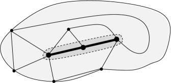
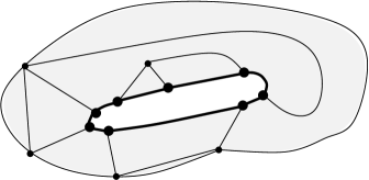
Figure 14: A CW-complex $X$ with open neighbourhood of a subcomplex $Y$ (left). The CW-complex $W$ for this choise of $X$ and $Y$ (right).

The closure $\overline{e^{n}}$ of any $n$-cell $e^{n}\subset X$ is a finite CW-subcomplex of $X$. For an internal $n$-cell $e^{n}\subset X\setminus Y$ the intersection $\overline{e}^{n}\cap Y$ is also a CW-subcomplex of $X$, which we can express as a union

$$\overline{e}^{n}\cap Y=A_{1}^{e^{n}}\cup A_{2}^{e^{n}}\cup\cdots A_{k}^{e^{n}}$$

of its path-components $A_{i}^{e^{n}}$. Each $A_{i}^{e^{n}}$ is a CW-subcomplex of $Y$.

Let us make the following simplifying assumption. When a space fails to meet the assumption it is sometimes possible to apply barycentric subdivision to offending top-dimensional cells (or possibly some less costly subdivision) in order to modify the CW structure so that it does satisfy the assumption.

Simplifying assumption: Let us suppose that each $A_{i}^{e^{n}}$ is contractible.

Under this assumption the CW-complex $W$ has precisely one internal $n$-cell $e^{n}$ for each cell $e^{n}\subset X\setminus Y$, and precisely one external $(n-1)$-cell

$$f^{e^{n}}_{A_{i}}$$

for each path-component $A_{i}$ of $\overline{e}^{n}\cap Y$.

The cellular chain complex $C_{\ast}W$ is generated in degree $n$ by the $n$-cells $e^{n}$ of $W$. By the homological boundary of $e^{n}$ we mean its image $de^{n}$ under the boundary homomorphism $d\colon C_{n}W\rightarrow C_{n-1}W$. The homological boundary $de^{n}$ is a sum of finitely many distinct $(n-1)$-cells each occuring with coefficient $\pm 1$. We’ll abuse terminology and say that $de^{n}$ is a sum of these distinct $(n-1)$ cells (without mentioning that coefficients are $\pm 1$ in the sum).

The homological boundary of an internal cell $e^{n}$ in $W$ is a sum of all the internal $(n-1)$-cells lying in $\overline{e}^{n}$ together with all external $(n-1)$-cells $f^{e^{n}}_{A_{i}}$ with $A_{i}$ a path-components of $\overline{e}^{n}\cap Y$. The homological boundary of an external $(n-1)$-cell $f^{e^{n}}_{A_{i}}$ is a sum of all those external $(n-1)$-cells $f^{e^{n-1}}_{B}$ with $e^{n-1}$ an $(n-1)$-cell of $\overline{e}^{n}$ and path-component $B$ of $\overline{e}^{n}\cap Y$ with $B\subseteq A_{i}$.

Algorithm 10.1 Excise an open tubular neighbourhood from a regular CW-complex.

1:A finite regular CW-complex $X$ and subcomplex $Y\subset X$ satisfying the above simplifying assumption.

2:A finite regular CW-complex $W$.

3:procedure 

4:     For each internal cell $e^{n}\subset X\setminus Y$ compute the CW-complex $\overline{e}^{n}\cap Y$ and express it as a union $e^{n}\cap Y=A_{1}^{e^{n}}\cup A_{2}^{e^{n}}\cup\cdots A_{k}^{e^{n}}$ of its path-components $A_{i}^{e^{n}}$. This determines the number of cells of each dimension in $W$.

5:     Create a list of empty lists $B=[[],[],\cdots,[]]$ of length $1+\dim X$.

6:     For $0\leq n\leq\dim X$ set $B[n+1]=[b_{1},b_{2},\cdots,b_{\alpha_{n}}]$ where $\alpha_{n}$ denotes the number of $n$-cells in $W$ and $b_{i}$ is a list of integers determining the $(n-1)$-cells with non-zero coefficient in the homological boundary of the $i$-th $n$-cell of $W$. In the ordering of $n$-cells it is convenient to order all internal cells before any external cell.

7:     Represent the data in $B$ as a regular CW-complex $W$ and return $W$.

8:end procedure

11 A homotopy classification of maps

Our original motivation for attempting computations of local cohomology is a classical result of Whitehead concerning the set $[W,X]_{\phi}$ of based homotopy classes of maps $f\colon W\rightarrow X$ between connected CW-complexes $W$ and $X$ that induce a given homomorphism $\phi\colon\pi_{1}W\rightarrow\pi_{1}X$ of fundamental groups. As mentioned in the Introduction, we assume that the spaces $W$, $X$ have preferred base points, that the maps $f$ preserve base points, and that base points are preserved at each stage of a homotopy between maps. The homotopy groups of a space $X$ are denoted by $\pi_{n}X$, $n\geq 0$. A chain map $\chi_{\ast}\colon C_{\ast}\widetilde{W}\rightarrow C_{\ast}\widetilde{X}$ between cellular chain complexes of universal covers is said to be $\phi$-equivariant if $\chi_{n}(gw)=\phi(g)\chi_{n}(w)$ for all $g\in\pi_{1}W$, $w\in C_{n}\widetilde{W}$, $n\geq 0$. Two such $\phi$-equivariant chain maps $\chi_{\ast},\psi_{\ast}\colon C_{\ast}\widetilde{W}\rightarrow C_{\ast}\widetilde{X}$ are said to be based chain homotopic if there exist $\phi$-equivariant homomorphisms $h_{i}\colon C_{i}\widetilde{W}\rightarrow C_{i+1}\widetilde{X}$ for $i\geq 0$, such that

$$\chi_{i}(w)-\psi_{i}(w)=d_{i+1}h_{i}(w)+h_{i-1}d_{i}(w)$$ (8)

for $w\in C_{i}\widetilde{W}$ and $h_{-1}=0$. Based chain homotopy is an equivalence relation and we denote by $[C_{\ast}\widetilde{W},C_{\ast}\widetilde{X}]_{\phi}$ the set of based chain homotopy classes of $\phi$-equivariant chain maps $C_{\ast}\widetilde{W}\rightarrow C_{\ast}\widetilde{X}$. The following theorem is proved in Whitehead (1949).

Theorem 5 (Whitehead).

Let $W,X$ be connected CW-complexes, and let $\phi\colon\pi_{1}W\rightarrow\pi_{1}X$ be a group homomorphism. Suppose that $W$ is of dimension $n$ and that $\pi_{i}X=0$ for $2\leq i\leq n-1$. Then there is a bijection

$$[W,X]_{\phi}\cong[C_{\ast}\widetilde{W},C_{\ast}\widetilde{X}]_{\phi}.$$

To derive Theorem 1 from Theorem 5 we need to establish a bijection $[C_{\ast}\widetilde{W},C_{\ast}\widetilde{X}]_{\phi}\cong H^{n}(W,H_{n}(\widetilde{X}))$. Let $W,X$ and $\phi$ satisfy the hypothesis of Theorem 1. Without loss of generality, we impose the additional hypothesis that both $W$ and $X$ have precisely one $0$-cell, say $e^{0}\in W$, $e^{\prime 0}\in X$, and that these $0$-cells are taken to be the base points. Furthermore, we identify cells of $W,X$ with free $\mathbb{Z}\pi_{1}$-generators of $C_{\ast}\widetilde{X},C_{\ast}\widetilde{W}$. Let $f\colon W\rightarrow X$ be a cellular map inducing $\phi$. Such a map $f$ exists because, by the theory of group presentations, the $2$-skeleta $W^{2}$, $X^{2}$ correspond to group presentations of $\pi_{1}W$, $\pi_{1}X$; the homomorphism $\phi$ is induced by at least one cellular map $f\colon W^{2}\rightarrow X^{2}$. This map of 2-skeleta extends to a cellular map $f\colon W\rightarrow X$ since $\pi_{i}X=0$ for $2\leq i\leq n-1$. Let $\chi_{\ast}\colon C_{\ast}\widetilde{W}\rightarrow C_{\ast}\widetilde{X}$ be the chain map induced by $f$. Note that $\chi_{\ast}$ is pointed in the sense that $\chi_{0}(e^{0})=e^{\prime 0}$. Let $[\chi_{\ast}]$ denote the based homotopy class of $\chi_{\ast}$. Then $[\chi_{\ast}]\in[C_{\ast}\widetilde{W},C_{\ast}\widetilde{X}]_{\phi}$. We choose (one such) $\chi_{\ast}$ as the preferred $\phi$-equivariant chain map.

Suppose that $\psi_{\ast}\colon C_{\ast}\widetilde{W}\rightarrow C_{\ast}\widetilde{X}$ is some other $\phi$-equivariant pointed chain map. Then $\chi_{0}=\psi_{0}$. Suppose that for some $0\leq k\leq n-2$ we have $\phi_{i}=\psi_{i}$ for $0\leq i\leq k$. Then for each free $\mathbb{Z}\pi_{1}W$-generator $e^{k}_{j}\in C_{k}\widetilde{W}$ we have $\chi_{k}(e^{k}_{j})-\psi_{k}(e^{k}_{j})\in\ker(d_{k}\colon C_{k}\widetilde{X}\rightarrow C_{k-1}\widetilde{X}$). Since $H_{k}(C_{\ast}\widetilde{X})=\pi_{k}(X)=0$ we can choose some element $h(e^{\prime k}_{j})\in C_{k+1}\widetilde{X}$ satisfying $\chi_{k}(e^{k}_{j})-\psi_{k}(e^{k}_{j})=d_{k+1}h(e^{\prime k}_{j})$. Here $h(e^{\prime k}_{j})$ is just our label for the chosen element. This defines a $\phi$-equivariant homomorphism $h\colon C_{k}\widetilde{W}\rightarrow C_{k+1}\widetilde{X}$.

We define a $\phi$-equivariant chain map $\psi^{\prime}_{\ast}\colon C_{\ast}\widetilde{W}\rightarrow C_{\ast}\widetilde{X}$ by setting $\psi^{\prime}_{i}=\psi_{i}$ $(i\neq k,k+1)$, $\psi^{\prime}_{k}=\chi_{k}$, $\psi^{\prime}_{k+1}=\psi_{k+1}+hd_{k+1}$. Then $\psi^{\prime}_{\ast}$ is based chain homotopic to $\psi_{\ast}$ and $\psi^{\prime}_{i}=\chi_{i}$ for $0\leq i\leq k+1$. By induction the based homotopy class $[\psi_{\ast}]$ is represented by a chain map $\psi_{\ast}$ satisfying $\psi_{i}=\chi_{i}$ for $0\leq i\leq n-1$. Using this representative we define the $\phi$-equivariant cocycle

$$C_{[\chi_{\ast}]-[\psi_{\ast}]}=\chi_{n}-\psi_{n}\colon C_{n}\widetilde{W}\rightarrow H_{n}(C_{\ast}\widetilde{X}).$$

For fixed $\chi_{\ast}$, the assignment $\psi_{\ast}\mapsto C_{[\chi_{\ast}]-[\psi_{\ast}]}$ induces the bijection $[C_{\ast}\widetilde{W},C_{\ast}\widetilde{X}]_{\phi}\cong H^{n}(W,H_{n}(\widetilde{X}))$ which proves Theorem 1.

12 Reproducibility of computations

All computations in the paper were obtained using GAP v4.11.0 and HAP v1.29 and Debian GNU/Linux 10 (buster) on a laptop with an i7–6500U CPU and 4GB of RAM. The code in Tables 1–4 has been stored as examples in HAP which can be run using the command

gap> HapExample("jsc2021-n");

for $n=1,2,3,4$. Two further examples relating to computations in the paper have also been stored in HAP. Timings for the examples, in hour:min:sec format, are as follows.

Example	Details	Time
jsc2021-1	Code of Table 1.	0:06:09
jsc2021-2	Code of Table 2. Requires jsc2021-1.	0:43:13
jsc2021-3	Code of Table 3.	0:18:36
jsc2021-4	Code of Table 4.	0:00:02
jsc2021-5	Establish that $X_{S}$, $X_{T}$ have identical integral homology and fundamental group. Requires jsc2021-3 & jsc2021-4.	0:00:06
jsc2021-6	Computations underlying Section 9.	0:04:08

13 Acknowledgments

The second author is grateful to the Irish Research Council for a postgraduate scholarship under project GOIPG/2018/2152. The authors thank the referee for helpful comments and for suggesting the inclusion of Section 12.

References

-
Artin (1925)
Artin, E., 1925. Zur Isotopie zweidimensionaler Flächen im .
Abh. Math. Sem. Univ. Hamburg 4 (1), 174–177.
URL https://doi-org.libgate.library.nuigalway.ie/10.1007/BF02950724 -
Brendel et al. (2015)
Brendel, P., Dłotko, P., Ellis, G., Juda, M., Mrozek, M., 2015. Computing
fundamental groups from point clouds. Appl. Algebra Engrg. Comm. Comput.
26 (1-2), 27–48.
URL http://dx.doi.org/10.1007/s00200-014-0244-1 -
Davit (2017)
Davit, E., 2017. Knots in 4d – part 3. Youtube.
URL https://www.youtube.com/watch?v=p5tPb5yN-CE -
Ellis (2019)
Ellis, G., 2019. An invitation to computational homotopy. Oxford University
Press, UK.
URL https://global.oup.com/academic/product/an-invitation-to-computational-homotopy-9780198832980 - Ellis (November 2019) Ellis, G., November 2019. HAP – Homological Algebra Programming, Version 1.21. (http://www.gap-system.org/Packages/hap.html).
-
Ellis and Fragnaud (2018)
Ellis, G., Fragnaud, C., 2018. Computing with knot quandles. J. Knot Theory
Ramifications 27 (14), 1850074, 18.
URL https://doi-org.libgate.library.nuigalway.ie/10.1142/S0218216518500748 -
Ellis and Hegarty (2014)
Ellis, G., Hegarty, F., 2014. Computational homotopy of finite regular
CW-spaces. J. Homotopy Relat. Struct. 9 (1), 25–54.
URL http://dx.doi.org/10.1007/s40062-013-0029-4 -
Forman (1998)
Forman, R., 1998. Morse theory for cell complexes. Adv. Math. 134 (1), 90–145.
URL http://dx.doi.org/10.1006/aima.1997.1650 - Forman (2002) Forman, R., 2002. A user’s guide to discrete Morse theory. Sém. Lothar. Combin. 48, Art. B48c, 35.
-
Fox (1954)
Fox, R. H., 1954. Free differential calculus. II. The isomorphism problem
of groups. Ann. of Math. (2) 59, 196–210.
URL https://doi-org.libgate.library.nuigalway.ie/10.2307/1969686 - GAP (2013) GAP, 2013. GAP – Groups, Algorithms, and Programming, Version 4.5.6. The GAP Group, (http://www.gap-system.org).
-
Hatcher (2002)
Hatcher, A., 2002. Algebraic topology. Cambridge University Press, Cambridge,
New York, autre(s) tirage(s) : 2003,2004,2005,2006.
URL http://opac.inria.fr/record=b1122188 -
Hempel (1984)
Hempel, J., 1984. Homology of coverings. Pacific J. Math. 112 (1), 83–113.
URL http://projecteuclid.org.libgate.library.nuigalway.ie/euclid.pjm/1102710101 - Jones (1988) Jones, D., 1988. A general theory of polyhedral sets and the corresponding -complexes. Dissertationes Math. (Rozprawy Mat.) 266, 110.
-
Kauffman and Faria Martins (2008)
Kauffman, L. H., Faria Martins, J. a., 2008. Invariants of welded virtual knots
via crossed module invariants of knotted surfaces. Compos. Math. 144 (4),
1046–1080.
URL https://doi.org/10.1112/S0010437X07003429 -
Krăźál et al. (2013)
Krăźál, M., Matoušek, J., Sergeraert, F., Dec. 2013.
Polynomial-time homology for simplicial Eilenberg–Maclane spaces. Found.
Comput. Math. 13 (6), 935–963.
URL https://doi.org/10.1007/s10208-013-9159-7 -
Martins (2007)
Martins, J. a. F., 2007. Categorical groups, knots and knotted surfaces. J.
Knot Theory Ramifications 16 (9), 1181–1217.
URL https://doi-org.libgate.library.nuigalway.ie/10.1142/S0218216507005713 -
Martins (2009)
Martins, J. F., 2009. The fundamental crossed module of the complement of a
knotted surface. Trans. Amer. Math. Soc. 361 (9), 4593–4630.
URL http://dx.doi.org/10.1090/S0002-9947-09-04576-0 -
Mazur (1959)
Mazur, B., 1959. On embeddings of spheres. Bull. Amer. Math. Soc. 65, 59–65.
URL https://doi.org/10.1090/S0002-9904-1959-10274-3 -
Ocken (1990)
Ocken, S., 1990. Homology of branched cyclic covers of knots. Proc. Amer. Math.
Soc. 110 (4), 1063–1067.
URL https://doi-org.libgate.library.nuigalway.ie/10.2307/2047757 -
Rees and Soicher (2000)
Rees, S., Soicher, L., 2000. An algorithmic approach to fundamental groups and
covers of combinatorial cell complexes. J. Symbolic Comput. 29 (1), 59–77.
URL http://dx.doi.org/10.1006/jsco.1999.0292 -
Satoh (2000)
Satoh, S., 2000. Virtual knot presentation of ribbon torus-knots. J. Knot
Theory Ramifications 9 (4), 531–542.
URL https://doi.org/10.1142/S0218216500000293 - Spanier (1981) Spanier, E., 1981. Algebraic Topology, corrected reprint of the 1966 original. Springer, New York.
- The Sage Developers (2019) The Sage Developers, 2019. SageMath, the Sage Mathematics Software System (Version 8.7.0). http://doc.sagemath.org/html/en/reference/homology/sage/homology/simplicial_set.html.
-
Trotter (1962)
Trotter, H. F., 1962. Homology of group systems with applications to knot
theory. Ann. of Math. (2) 76, 464–498.
URL https://doi.org/10.2307/1970369 -
Čadek et al. (2014a)
Čadek, M., Krčál, M., Matoušek, J., Sergeraert, F.,
Vokřínek, L., Wagner, U., Jun. 2014a. Computing all
maps into a sphere. J. ACM 61 (3), 17:1–17:44.
URL http://doi.acm.org/10.1145/2597629 - Čadek et al. (2014b) Čadek, M., Krčál, M., Matoušek, J., Vokřínek, L., Wagner, U., 2014b. Polynomial-time computation of homotopy groups and Postnikov systems in fixed dimension. SIAM Journal on Computing 43 (5), 1728–1780.
- Whitehead (1949) Whitehead, J. H. C., 1949. Combinatorial homotopy. II. Bull. Amer. Math. Soc. 55, 453–496.
- Whitehead (1950) Whitehead, J. H. C., 1950. Simple homotopy types. Amer. J. Math. 72, 1–57.
-
Zeeman (1961)
Zeeman, E. C., 1961. Knotting manifolds. Bull. Amer. Math. Soc. 67, 117–119.
URL https://doi.org/10.1090/S0002-9904-1961-10529-6