Cloud Properties and Correlations with Star Formation in Numerical Simulations of the Three-Phase ISM

Abstract

We apply gravity-based and density-based methods to identify clouds in numerical simulations of the star-forming, three-phase interstellar medium (ISM), and compare their properties and their global correlation with the star formation rate over time. The gravity-based method identifies bound objects, which have masses $M\sim 10^{3}-10^{4}\;M_{\odot}$ at densities $n_{\mathrm{H}}\sim 100\;{\rm cm}^{-3}$, and traditional virial parameters $\alpha_{v}\sim 0.5-5$. For clouds defined by a density threshold $n_{\rm H,min}$, the average virial parameter decreases, and the fraction of material that is genuinely bound increases, at higher $n_{\rm H,min}$. Surprisingly, these clouds can be unbound even when $\alpha_{v}<2$, and high mass clouds ($10^{4}-10^{6}\;M_{\odot}$) are generally unbound. This suggests that the traditional $\alpha_{v}$ is at best an approximate measure of boundedness in the ISM. All clouds have internal turbulent motions increasing with size as $\sigma\sim 1\;{\rm km}\;{\rm s}^{-1}(R/\;{\rm pc})^{1/2}$, similar to observed relations. Bound structures comprise a small fraction of the total simulation mass, with star formation efficiency per free-fall time $\epsilon_{\mathrm{ff}}\sim 0.4$. For $n_{\rm H,min}=10-100\;{\rm cm}^{-3}$, $\epsilon_{\mathrm{ff}}\sim 0.03-0.3$, increasing with density. Temporal correlation analysis between $\mathrm{SFR}(t)$ and aggregate mass $M(n_{\rm H,min}{};t)$ at varying $n_{\rm H,min}$ shows that time delays to star formation are $t_{\mathrm{delay}}\sim t_{\mathrm{ff}}(n_{\rm H,min})$. Correlation between $\mathrm{SFR}(t)$ and $M(n_{\rm H,min};t)$ systematically tightens at higher $n_{\rm H,min}$. Considering moderate-density gas, selecting against high virial parameter clouds improves correlation with SFR, consistent with previous work. Even at high $n_{\rm H,min}$, the temporal dispersion in $(\mathrm{SFR}-\epsilon_{\mathrm{ff}}M/t_{\mathrm{ff}})/\langle\mathrm{SFR}\rangle$ is $\sim 50\%$, due to the large-amplitude variations and inherent stochasticity of the system.

1 Introduction

The interstellar medium is hierarchically structured. The densest entities are individual prestellar cores, which generally are found within filaments or clumps in giant molecular clouds (GMCs) (André et al., 2014; Dobbs et al., 2014); the GMCs may be part of molecular/atomic complexes, and are typically found within spiral arms, arm spurs/feathers, or sheared flocculent features (Elmegreen, 1980; La Vigne et al., 2006). At any given time within a galaxy, a distribution of GMCs with various properties exists, and each forms stars according to the distribution of clumps and cores within it. To understand the intermediate scale between parsecs and kiloparsecs, the properties of GMCs must be understood, and it is of particular interest to investigate whether the characteristics of a GMC may be used to predict its star formation rate.

There is a long history of characterizing ISM structures in observations. Molecular lines, dust extinction, and dust emission maps are used to identify regions with high column density or number density. These density proxies are a convenient and readily available way to identify structures, and from these measurements distributions of cloud sizes and masses can be obtained. In addition to measuring column densities from molecular or dust emission, line emission is used to trace velocities of gas, and from this the kinetic energy content of the structures can be estimated. For example, based on CO surveys, GMCs in the Milky Way have masses $10^{4}-10^{6}\;M_{\odot}$, radii between $10-50\;{\rm pc}$, velocity dispersion between $1-7\;{\rm km}\;{\rm s}^{-1}$, and a linewidth-size relationship of $\sigma_{1D}=0.9\;{\rm km}\;{\rm s}^{-1}(R/\;{\rm pc})^{1/2}$ (Solomon et al., 1987; Blitz, 1993; Heyer & Dame, 2015), and properties of resolved GMCs in nearby galaxies are similar (Bolatto et al., 2008).

By combining an estimate of the mass, size, and velocity dispersion, an estimate of the virial parameter $\alpha_{v}\equiv 2E_{\rm k}/|E_{\rm g}|$ (for kinetic energy $E_{\rm k}$ and gravitational energy $E_{\rm g}$) can be obtained (e.g. Roman-Duval et al., 2010; Hernandez & Tan, 2015). Virial parameter estimates from observations typically adopt $|E_{\rm g}|=3GM^{2}/(5R)$ for the gravitational energy, as would apply for an isolated, uniform-density sphere, where the effective radius is empirically computed from projected area as $R=(A/\pi)^{1/2}$. Although the case of ellipsoidal structures has been considered (Bertoldi & McKee, 1992), more general effects from nonspherical cloud geometry are not generally taken into account (even though the filamentary nature of the ISM makes many clouds quite elongated); non-sphericity tends to reduce gravitational binding. Internal stratification is sometimes taken into account by assuming a power-law density profile, which can increase the estimated $|E_{\rm g}|$ by up to a factor $\sim 2$ (Hernandez & Tan, 2015).

Based on the simplest spherical estimate, clouds are considered “bound” if the estimated virial parameter $\alpha_{v}\equiv 5\sigma^{2}R/(GM)$ is less than or equal to 2, where $\sigma$ is the line-of-sight velocity dispersion. However, traditional estimates of gravitational binding energy are problematic even beyond the assumptions of homogeneity and spherical geometry because the “isolated cloud” estimate of $|E_{\rm g}|$ does not properly take into account neighboring structures. For a given local gravitational potential minimum at the center of a cloud, tidal forces set the effective zero of the gravitational potential not at infinite distance but along the first potential contour that has a saddle point – equivalent to the Roche lobe for the case of two spherical bodies. As a result, tidal forces effectively decrease gravitational binding energy $|E_{\rm g}|$ of dense regions in close proximity to other dense regions, which is common because of the hierarchical structure of density variations. In addition, simple virial parameter estimates neglect magnetic contributions to support, which can significantly add to the numerator (McKee et al., 1993; Heiles et al., 1993). Although simple virial parameter estimates are inexact, they are often used to assess whether a structure is a likely candidate for star formation.

Star formation is observed to take place within the densest structures at the smallest scale within the ISM hierarchy, and it is important to understand what dynamical processes lead to the onset of gravitational collapse, and what controls the rate of star formation within a given level of the hierarchy. More generally, it is of interest to understand how star formation timescales are related to the properties and corresponding timescales of gaseous structures. Because star formation involves gravity, the most commonly invoked reference timescale is the free-fall collapse time,

$$t_{\mathrm{ff}}=\left(\frac{3\pi}{32G\rho}\right)^{1/2},$$ (1)

where $\rho$ is the gas density. Perhaps the simplest way to characterize the relationship between star formation and gas properties is via the star formation efficiency per free-fall time (Krumholz & McKee, 2005; Krumholz & Tan, 2007), defined as

$$\epsilon_{\mathrm{ff}}\equiv\frac{\dot{M}_{*}}{M/t_{\mathrm{ff}}},$$ (2)

where $t_{\mathrm{ff}}$ is the free-fall time at the mean density of the gas contributing to $M$, and $\dot{M}_{*}$ is the star formation rate (SFR). Other relevant timescales include the flow crossing time across a structure that is supported by turbulent stresses, and the sound crossing time for a structure that is supported by thermal pressure. A class of theoretical models for star formation suggests that in turbulent clouds, there is a critical density $\rho_{\mathrm{crit}}$ above which collapse occurs within a free-fall time, with $\rho_{\mathrm{crit}}$ depending on the the ratios of kinetic to gravitational energy (virial parameter), turbulent to thermal velocity (Mach number), and thermal to magnetic pressure (plasma beta parameter) (Krumholz & McKee, 2005; Padoan & Nordlund, 2011; Hennebelle & Chabrier, 2011; Federrath & Klessen, 2012; Padoan et al., 2014). The underlying physical concept behind the idea of a critical density is that the density must be high enough that thermal pressure and magnetic stresses cannot support against collapse, and that the collapse time is shorter than the timescale for shear to tear apart a structure.

In addition to theoretical models, direct numerical simulations have been used to characterize the dependence of SFRs on gas properties. One idealized type of setup employs simulations with isothermal, self-gravitating gas, in which turbulence is driven in Fourier space. From a large set of driven-turbulence simulations, Padoan et al. (2012) suggested that $\epsilon_{\mathrm{ff}}$ depends primarily on the ratio of flow crossing time to free-fall time as

$$\epsilon_{\mathrm{ff}}\propto\exp(-1.6t_{\mathrm{ff}}/t_{\mathrm{dyn}}).$$ (3)

where $t_{\rm dyn}=R/\sigma_{3D}=R/(\sqrt{3}\sigma_{1D})$ is the flow crossing time for system size $2R$ ($=L$, the simulation box size for Padoan et al. (2012)). For a uniform spherical cloud, the timescale ratio can be related to the virial parameter by

$$\left(\frac{t_{\mathrm{ff}}}{t_{\mathrm{dyn}}}\right)^{2}=\frac{3\pi^{2}}{40}\alpha_{v};$$ (4)

thus, these simulations suggest a strong suppression of star formation at high $\alpha_{v}$.

Idealized simulations have the advantage of carefully controlled conditions, but the disadvantages that the turbulence is driven in an artificially prescribed manner to maintain a fixed overall turbulent amplitude, and that the processes leading to cloud formation and destruction are not followed. In reality, GMCs form due to a combination of large-scale ISM flows (including turbulence, shear, and epicyclic motion) and gravity (both stellar gravity and self-gravity) that lead to collection of material from a large volume, as mediated by thermal and magnetic pressure, and a change from atomic to molecular phase as gas cools. Turbulence on scales less than the scale height of the warm-cold ISM likely originates primarily due to the feedback from young stars (Mac Low & Klessen, 2004; McKee & Ostriker, 2007; Elmegreen & Scalo, 2004), whether inherited from a GMC’s formation stage or produced internally. Considering that GMCs live for at most a few turbulent crossing times or free-fall times (Kawamura et al., 2009; Kruijssen et al., 2019), it is not clear that internal GMC conditions can control star formation in a way that is entirely divorced from their formation and destruction processes.

In recent years, (magneto)-hydrodynamic simulations have been used to follow the star-forming multiphase ISM in kpc-size regions at high resolution. In these simulations, massive self-gravitating clouds naturally condense out of the diffuse gas, and within these clouds localized collapse occurs that represents star cluster formation (Gatto et al., 2017; Iffrig & Hennebelle, 2017; Kim & Ostriker, 2017; Kannan et al., 2018; Colling et al., 2018). By modeling the return of energy (representing radiative heating and supernova explosions) from these cluster particles to their surroundings, a self-consistent, self-regulated state can be reached in which all thermal phases of the ISM are represented, and a hierarchy of structures is naturally created. While the large-scale time-averaged SFR adjusts such that feedback provides the energy and momentum needed to maintain overall equilibrium in the ISM as a whole (Ostriker et al., 2010; Ostriker & Shetty, 2011; Kim et al., 2011, 2013), the collapse to make individual star clusters depends on local conditions in overdense clouds. Simulations of this kind present an opportunity to evaluate the role of gravity in binding ISM structures that are part of a complex environment, and to assess common practices for estimating gravitational boundedness. In addition, simulations of this kind afford a realistic setting to test theoretical ideas regarding the role of gravitational boundedness in controlling SFRs.

In this paper, we use a large-scale ISM simulation produced in the TIGRESS framework (Kim & Ostriker, 2017) to characterize the properties of dense structures and their relationship to star formation. Our structural decomposition analysis includes methods that are similar to typical observational practices, in which objects are defined based on density or column density. For sets of objects defined by different density thresholds, we compute statistics of mass, size, and velocity dispersion, which allows us to compute “empirical” virial parameters and linewidth-size relations. We compute both traditional virial parameters (only kinetic energy) and virial parameters including thermal and magnetic energy. In addition, we apply another method of defining structures based on contours of the gravitational potential (rather than density contours). In this method we identify bound objects as regions where the kinetic, thermal, and magnetic energy are sufficiently low compared to the gravitational energy (computed relative to a tidally-defined potential contour). These two analyses allow us to relate traditional virial parameter estimates for objects to measurements of gravitational binding that directly take into account nonspherical geometry, internal stratification, and tidal forces. We shall show that traditional virial parameter estimates can significantly under- or over-state the true boundedness of ISM structures.

To study the relationship between gas and star formation, we use correlations between the temporal history of the SFR and the mass of gas in different categories of objects, including objects defined by density thresholds and objects defined by being gravitationally bound. In this way, we are able to measure how $\epsilon_{\mathrm{ff}}$ varies as a function of density and what $\epsilon_{\mathrm{ff}}$ is for objects that are gravitationally bound (also allowing for different treatments of surface terms). We are also able to measure time delays between the availability of a mass reservoir and the star formation burst that it produces. We use correlation analysis to quantify the relative predictive power of different star formation models that depend on the traditional virial parameter, and on our more sophisticated assessment of gravitational binding.

The plan of this paper is as follows. In Section 2 we describe our analysis methods, including how we identify bound objects (Section 2.1), the properties we measure for bound objects and for density-defined objects (Section 2.2), and how we conduct time-series correlation analyses (Section 2.3); Section 2.4 summarizes our methods and Section 2.5 describes the primary TIGRESS simulation that we analyze. Section 3 presents an overview of structure (Section 3.1) and results of our analyses, including statistics of object properties (Section 3.2) and time series correlation studies (Section 3.3), with a summary of trends in the values of $\epsilon_{\mathrm{ff}}$ and levels of correlations for various ways of selecting gas in Section 3.4. In Section 4 we summarize our results and discuss connections with other current theory and observations.

2 Methods

In this paper, we analyze the properties of dense and bound gas structures, and investigate the relationship between the material in these structures and the star formation rate, as applied to the fiducial TIGRESS model described in Kim & Ostriker (2017). The methods we develop, described in some detail here, are quite general and can be applied to other numerical simulation data. With some modifications to allow for projected rather than fully three-dimensional information, our methods can also be applied to observed data sets.

We begin by describing methods for identifying objects based on density isosurfaces or on the gravitational potential in comparison to the kinetic, thermal, and magnetic energy densities (Section 2.1); additional technical details of the algorithm are described in Appendix A. We also describe how we quantify object properties including mass, size, velocity dispersion, and virial parameter (Section 2.2). We then describe our use of time series to compare the simulated SFR to the history of mass per free-fall time for different categories of objects (Section 2.3); this involves fitting for optimal time delay and efficiency and Bayesian inference to test models for the dependence on virial parameter. Finally, in Section 2.5 we briefly summarize the numerical implementation and parameters of the TIGRESS model to which we have applied our analysis.

2.1 Bound Objects

To motivate our procedure for identifying gravitationally bound structures, consider what is bound in the Solar system. For example, a pebble on Earth is bound to the Earth, the Earth-Moon system, the Sun, and the Galaxy, but is not bound gravitationally to a nearby pebble. To make this determination, both the gravitational potential contours and the relative velocities of the structures involved are needed; a pebble as well as its neighbors mutually lie within the Earth’s gravitational potential as limited by the Moon’s tidal force, and do not have high enough velocities that they could find themselves on the Moon or escape entirely from the Solar system. Thus, we consider the pebble as part of the Earth.

For application to the ISM and star formation, boundedness can also have a characteristic scale dependence. Matter on larger scales tends to have a higher internal kinetic energy ($\sigma^{2}\propto L$) from the scaling properties of turbulence, but also tends to be increasingly bound by the gravitational potential ($GM/R\sim\rho{}L^{2}$). Depending on the scale dependence of the density, there may be a hierarchy of boundedness, with bound structures nested within other bound structures.

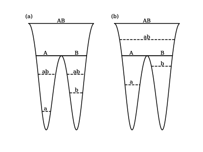
With the above motivation, we identify a hierarchy of structures in our ISM simulations based on contours of the gravitational potential, and bound structures based on the energy of fluid elements relative to the structure tree. The first level of the gravitational tree is comprised of structures enclosed by isocontours that surround a single minimum. Each successive level is comprised of material within isocontours enclosing distinct sets of minima whose largest enclosing isocontours are in contact. That is, branches merge into a new object when their isocontours are in contact. This means that each object in the tree can be uniquely identified with a critical point in the gravitational potential, where isocontours come into contact. Figure 1 provides a schematic illustration of this procedure.

Figure 1: Schematic of HBPs (upper case) and associated HBRs (lower case) as level sets within gravitational wells, plotting gravitational energy against spatial coordinate. Each HBR is bound relative to its associated HBP. For example, on both left and right “a” represents material interior to an isocontour of the gravitational well such that the HBR has 0 total energy, bound relative to the gravitational contour “A.” Similarly, “b” is bound relative to “B.” The regions “a” and “b” are therefore both HBRs. On the left, we show an example of a region “ab” which is invalid as an HBR because it consists of two non-contiguous parts. On the right, we show an example of a contiguous HBR “ab” which merges “a” and “b.” We are generally interested in only the largest HBRs in any hierarchy, so on the right we would remove the objects “a” and “b” from further consideration. This schematic also illustrates that each HBP object can be identified by a critical point of the potential: “A” and “B” are associated with their respective local minima, and “AB” is associated with the central local maximum.

At each level in the gravitational potential contour tree, we denote the object enclosed within a closed contour as a hierarchical binding parent (HBP). Within each of these objects, we denote some subset of the gas as a hierarchical bound region (HBR). The HBR is the set of cells for which the total energy (kinetic, thermal, magnetic, gravitational) of the region is 0. In this calculation, we assign a gravitational binding energy to each cell based on the difference between its gravitational potential ($\Phi$) and the isocontour surface of the HBP ($\Phi_{0}$); i.e. the contribution to the gravitational energy of the HBR is $(\Phi-\Phi_{0})\rho dx^{3}$. Hence, the HBP is responsible for binding these HBR cells. Cells are added to a candidate HBR in order of gravitational potential depth (deepest first). For the contribution to kinetic energy, the center of mass (COM) velocity of the subset of cells is subtracted out first. Within a given HBP, the most massive bound subset of cells is taken as the HBR; if no cells are bound, there is no HBR.

In the above definition, we have not considered any effects from thermal or turbulent stresses on the surface (defined by an equipotential) of objects. Because the dynamics of turbulent systems are complex, surface stresses could in principle either act to compress and help bind structures (e.g. for a converging flow) or act to disperse and unbind structures (e.g. for a shear flow). While the complex dynamics makes it impossible to decide between these alternatives in a general sense, we can still investigate the potential magnitude of the effects that surface stresses may have. To do this, we begin by averaging the kinetic (${\cal E}_{\rm k}$), thermal (${\cal E}_{\rm th}$), and magnetic (${\cal E}_{\rm B}$) energy density over the surface $\Omega$ of the HBP ($N$ cells) to compute the mean surface energy density

$${\cal E}_{\rm\Omega}=\frac{1}{N}\sum\limits_{i\in\Omega}({\cal E}_{\rm k,i}+{\cal E}_{\rm th,i}+{\cal E}_{\rm B,i}).$$ (5)

Here, ${\cal E}_{\rm k,i}$ is the kinetic energy density computed relative to the center of mass velocity of the surface cells.

We then define “HBR+1” and “HBR-1” objects, where the object HBR$\pm$1 is the set of cells satisfying

$$\sum\limits_{i\in\mathrm{HBR\pm 1}}{\cal E}_{\rm k,i}+{\cal E}_{\rm th,i}+{\cal E}_{\rm B,i}<\sum\limits_{i\in\mathrm{HBR\pm 1}}(\Phi_{0}-\Phi_{i})\rho_{i}\pm{{\cal E}_{\rm\Omega}},$$ (6)

and now ${\cal E}_{\rm k,i}$ is the kinetic energy density computed relative to the center of mass velocity of the HBR$\pm 1$ cells. Clearly, HBR+1 will be more massive than the corresponding HBR identified without the surface energy terms, because the criterion for including cells becomes less restrictive by adding ${\cal E}_{\rm\Omega}$ on the right-hand side. Similarly, HBR-1 will be less massive than the corresponding HBR. This procedure could be generalized by adding or subtracting arbitrary multiples of ${\cal E}_{\rm\Omega}$, but for comparison purposes we have found HBR-1, HBR, HBR+1 suffice. We can think of HBR+1 objects as structures in which surface stresses are treated as helping to bind material; HBR-1 objects are those where surface stresses are treated as reducing binding. Physically, addition of ${\cal E}_{\rm\Omega}$ on the right-hand side in HBR+1 is equivalent to only considering the excess of ${\cal E}_{\rm k}$, ${\cal E}_{\rm th}$, and ${\cal E}_{\rm B}$ over “ambient” values when computing total energy.

Subsequently, we will test the correlation of HBR and HBR$\pm$1 objects with respect to the star formation rate; if surface terms play an important physical role, we might expect this to be reflected in the relative correlations with SFRs that we measure.

In the hierarchical contour tree, a nested sequence of HBPs is uniquely defined by critical points in the equipotential, e.g. in Figure 1 “A” and “B” are nested within “AB”. At each level of the tree, HBRs can be identified with respect to the corresponding HBPs. An additional requirement for HBR (and HBR$\pm 1$) objects to be considered valid is spatial compactness. Physically, we impose this requirement because a “divided” HBR within a single HBP could not be trusted to form a contiguous object.

The case of a non-contiguous HBR occurs when the COM velocity of the HBP is significantly different from that of its HBP branches, while the surface potential of the HBP is not significantly higher than that of its branches (this difference is equivalent to the difference between the HBP surface and the HBP originating critical point). Then, in this scenario, considering the HBP as a whole increases the kinetic energy without sufficiently increasing the depth of the binding gravitational well, resulting in separate regions that are unbound relative to each other but may be individually self-bound. Figure 1 shows an example of a contiguous vs. non-contiguous HBR.

Both HBPs and HBRs are grown contiguously from cells of decreasing potential depth, so a non-contiguous HBR would only form from an HBP with multiple local minima and correspondingly multiple HBP branches. The separate HBR subregions are each a subset of cells from one of those separate HBP branches, which meet at the critical point identified with the origin of the HBP. Hence, in our tree construction it suffices to check that the HBR of an HBP contains the critical point identifying that HBP, which is a convenient guarantee that the HBR is contiguous.

We have so far described a process of building a contour tree of gravitational potential isocontours. Each isocontour defines an HBP hosting an HBR (which may be empty, or may be non-contiguous). Because HBPs and HBRs are nested, one can consider levels in the hierarchy separately (in which case given fluid elements are counted at each level they appear), or one may apply a merging or pruning criterion to objects to “flatten” the hierarchy, such that each fluid element appears in at most a single object.

We are interested in regions self-bound on each scale. An HBP may bind a contiguous region of mass but have children binding non-contiguous regions. This is analogous to a larger scale self-bound system (like a galaxy) containing subregions that are not self-bound (an unbound GMC, with separate bound subregions, would be a non-contiguous HBR). To enforce that every level of the hierarchy is self-bound, we build the HBR tree from the HBP tree bottom-up, starting with leaf HBPs around individual local minima. A parent HBP is only evaluated (computing its HBR) if all its children HBPs were evaluated and host contiguous HBR. If an HBR is evaluated and contiguous, it replaces its branch HBRs, thus becoming a leaf node of the subset of the full HBR tree. The leaf nodes of the subset of the full HBR tree are considered to be star-forming regions.

This method naturally selects the largest scale candidates for contiguous collapse and hence star formation, and are robust to small-scale fluctuations in the gravitational potential (for example, the point-potentials of star particles). Furthermore, we note that changes over time in the gravitational potential structure can cause rapid changes in the population of leaf nodes of the contour tree. As objects disperse, merge, or evolve, critical points are created, destroyed, and relocated. Leaf nodes can be sensitive to such changes in the gravitational structure, but contiguous HBRs are more robust. For example, a dispersing or merging object smoothly transitions to or from being considered as multiple HBRs vs. a single HBR, because the relevant parameter is the total energy content, which (roughly) continuously changes.

We also checked the approach of building the HBR top-down, allowing a given HBR to contain non-contiguous HBRs, essentially allowing gas to be bound under any viable isocontour. This method produces contiguous HBRs that are as massive as possible.

Even with the above definitions, additional choices can be made in computing contiguous HBRs. We varied a single choice at a time to study their effects. For example, the star particle potential contribution to the potential could either be included or excluded. However, we found that including the star particle potential did not produce a significant quantitative effect on our results. The most significant difference we found was when building the HBR tree top-down: we found that in certain simulation snapshots (a few per cent of the time) where the mass happened to coalesce in a single region, the fraction of “bound mass” spiked by an order of magnitude. For the rest of this paper, when we refer to “HBR” the choices adopted are: building the HBR tree from the bottom-up, excluding the star particle potential, and ignoring surface stresses. We have found that that considering surface stresses can have a large effect, and we report results separately for objects identified as HBR$\pm 1$, as above. Inclusion of surface stresses as HBR+1 can lead to an order of magnitude more mass being considered “bound.” However, as we shall show, this does not have a strong effect on the correlation between star formation and “bound” mass over time.

2.2 Object Definition and Properties

After computing HBRs from the gravitational potential structure and fluid properties (density, kinetic energy, thermal energy, magnetic energy), we have a collection of objects, each of which contains a number of simulation cells.

There are also other means of identifying potentially star-forming objects that are closer to traditional observational methods that use molecular tracers that may have a characteristic threshold density, or dust emission/extinction maps with a minimum column. Here, we shall apply number density thresholds ($n_{\rm H,min}=$ 10, 30, and 100 $\;{\rm cm}^{-3}$) to identify contiguous regions where the number density $n_{\mathrm{H}}>n_{\rm H,min}$, referring to these regions as “$n_{\rm H,min}$ objects.” We also treat the set of HBPs for HBRs as objects.

We shall analyze HBRs, HBPs, and $n_{\rm H,min}$ objects in similar ways, both in terms of their properties and their relation to star formation. For each set of object categories in any simulation snapshot, we use member cells to calculate each object’s mass, volume, free-fall time from its mean (volume-weighted) density, and a mass per free-fall time.

For HBR and $n_{\rm H,min}$ objects we compute individual virial parameters $\alpha_{v}$. We compute the thermal energy density ${\cal E}_{\rm th}={\cal P}/(\gamma-1)$ for pressure ${\cal P}$ using $\gamma=5/3$. With momentum density $\mathbf{p}=\rho\mathbf{v}$ and center-of momentum velocity ${\bf v}_{\rm COM}$, the kinetic energy density is ${\cal E}_{\rm k}=(1/2)(|\mathbf{p}|^{2}/\rho{}-\rho{}\mathbf{v}_{\rm COM}^{2})$, while magnetic energy density is ${\cal E}_{\rm B}=|\mathbf{B}|^{2}/8\pi$ for magnetic field $\mathbf{B}$. These are summed over cells for each object to define the total kinetic, thermal, and magnetic energy $E_{\rm k}$, $E_{\rm th}$, and $E_{\rm B}$, respectively. We define an effective object radius $R$ from each object’s volume via $V=(4\pi{}/3)R^{3}$, and then define an estimated gravitational self-binding energy as

$$E_{\rm g}\equiv\frac{(3/5)GM^{2}}{R}$$ (7)

using the total object mass $M$. We note that this is not the true gravitational binding energy, but we adopt this definition for the purpose of comparison with standard practices in the field which assume isolated objects. With the above definitions, we set

$$\alpha_{v} \equiv 2\frac{E_{\rm k}}{E_{\rm g}}$$ (8)

$$\alpha_{\rm v,total} \equiv 2\frac{E_{\rm k}+E_{\rm th}+E_{\rm B}}{E_{\rm g}};$$ (9)

while the former is used most often in the literature under the assumption that kinetic energy dominates over both thermal and magnetic, the latter is more general. We also examine the separate energy components of objects.

For each $n_{\rm H,min}$ object, we find the mass fraction of cells that are also within HBRs. This allows us to examine the overlap between a method of identifying ISM structures (and possible star-forming regions) that is simple but easily applied, and a method that is sophisticated and physically motivated, but not directly applicable in observations. This mass fraction is also the probability of gas being bound given the observation that it is high density ($P(\rm bound|\rm dense)$). We colloquially refer to this as the “bound fraction.”

2.3 Time Series Analysis

A question of significant interest is the detailed correlation in time between the mass in identifiable star-forming structures and the actual star formation rate (SFR). To investigate this question, for each simulation snapshot and object type defined as described in Sections 2.1 and 2.2, we sum the mass, volume, and mass per free-fall time of all objects of that type within the snapshot. This procedure provides a set of time series (representing the ratio of mass per free-fall time for selected gas subsets) that we can use to test the connection to time-dependent star formation rate $\mathrm{SFR}(t)$.

To create time series for comparison to $\mathrm{SFR}(t)$, we also consider the collective material above minimum gas surface density thresholds $\Sigma_{0}=$ 10, 30, and 100 $\;M_{\odot}\;{\rm pc^{-2}}$. For each threshold and for each simulation snapshot, we compute the mass above the threshold, the volume ($n_{\rm H,min}$ objects only), and mass per free-fall time. For the free-fall time, we use a mass-weighted average density. For logarithmic bins of number density of half-decade width, we also compute the snapshot mass, volume, and mass per free-fall time, using the volume-weighted average density. This average density tends to be the lower edge of the bin when looking at the high density side of the distribution.

We compute the SFR at any given time $t$ by taking the total mass of all star particles whose age $t_{*}$ is less than some maximum age $t_{*,\rm max}$, and dividing by that age:

$$\rm{SFR}(t)=\sum\limits_{t_{*}<t_{*,\rm max}}M_{*}/t_{*,\rm max}$$ (10)

This is observationally motivated but also naturally smooths the SFR time series. This also introduces a delay shift of $t_{*,\rm max}/2$ in the time series relative to the simulation because mass that has formed stars at a given time $t$ contributes equally to the SFR at later times until $t+t_{*,\rm max}$, with midpoint centered on $t+t_{*,\rm max}/2$. As long as only young stars are considered and $t_{*,\rm max}$ is small, these effects are not problematic.

We use time series comparisons to compute the star formation efficiency per free-fall time (Equation 2) for each subset of the gas. For comparison to $\mathrm{SFR}(t)$, we use the individual time series ${M/t_{\mathrm{ff}}}$ from each defined gas subset (e.g. HBR, HBP, number density thresholds, number density bins, surface density threshold). Note that the typical density and free-fall time of a given definition do not significantly change over time, so correlating $\mathrm{SFR}$ with total mass per free-fall time ${M/t_{\mathrm{ff}}}$ is similar to correlating $\mathrm{SFR}(t)$ with the total mass $M(t)$ in a defined subset.

We treat our time series of simulation snapshots as a set of 2-D samples in $\mathrm{SFR}$ and ${M/t_{\mathrm{ff}}}$, and apply a simple linear regression to estimate $\epsilon_{\mathrm{ff}}$ using the model $\mathrm{SFR}=\epsilon_{\mathrm{ff}}{M/t_{\mathrm{ff}}}$. Hence, our inferred $\epsilon_{\mathrm{ff}}$ is simply

$$\epsilon_{\mathrm{ff}}=\frac{\sum_{N}\mathrm{SFR}_{i}({M/t_{\mathrm{ff}}})_{i}}{\sum_{N}({M/t_{\mathrm{ff}}})_{i}^{2}}=\frac{\langle(\mathrm{SFR}){M/t_{\mathrm{ff}}}\rangle}{\langle({M/t_{\mathrm{ff}}})^{2}\rangle}$$ (11)

with standard error in the fitted coefficient

$$\Delta\epsilon_{\mathrm{ff}}{}^{2}=\frac{1}{N-2}\frac{\sum_{N}\Delta{}\mathrm{SFR}_{i}^{2}}{\sum_{N}\left({M/t_{\mathrm{ff}}}_{i}-\langle{M/t_{\mathrm{ff}}}{}\rangle\right)^{2}}$$ (12)

where

$$\Delta\mathrm{SFR}_{i}=\mathrm{SFR}_{i}-\epsilon_{\mathrm{ff}}{}{M/t_{\mathrm{ff}}}_{i}$$ (13)

and $\langle{M/t_{\mathrm{ff}}}\rangle=(1/N)\sum_{N}({M/t_{\mathrm{ff}}})_{i}$. We note that the uncertainty in the inferred $\epsilon_{\mathrm{ff}}$ from Equation 12 will tend to decrease with increasing sample size.

The normalized variance in the error of the “data” SFR compared to the “model” $\epsilon_{\mathrm{ff}}M/t_{\mathrm{ff}}$ is then

$$\sigma_{\Delta\mathrm{SFR}/\langle\mathrm{SFR}\rangle}^{2}=\frac{1}{N-1}\frac{\sum_{N}\Delta\mathrm{SFR}_{i}^{2}}{\langle\mathrm{SFR}\rangle^{2}}.$$ (14)

We interpret a smaller normalized error $\sigma_{\Delta\mathrm{SFR}/\langle\mathrm{SFR}\rangle}$ as a stronger relationship between SFR and ${M/t_{\mathrm{ff}}}$. Note that the covariance and Pearson correlation coefficient between two variables $X$ and $Y$ both increase with a term $E[XY]$. The standard error increases with $\Delta\mathrm{SFR}_{i}^{2}=\mathrm{SFR}_{i}^{2}+\epsilon_{\mathrm{ff}}^{2}({M/t_{\mathrm{ff}}})_{i}^{2}-2\epsilon_{\mathrm{ff}}\mathrm{SFR}_{i}({M/t_{\mathrm{ff}}})_{i}$, hence decreasing with $E[(\mathrm{SFR}){M/t_{\mathrm{ff}}}]$. Thus, qualitatively, a smaller standard error corresponds to a larger covariance or correlation coefficient, and demonstrates a stronger dependence of SFR on ${M/t_{\mathrm{ff}}}$.

The above approach has the strength of being a statistically uncontroversial way to consistently estimate both $\epsilon_{\mathrm{ff}}$ and the strength of the relationship between SFR and ${M/t_{\mathrm{ff}}}$. It also benefits from giving more weight to simulation snapshots with more ${M/t_{\mathrm{ff}}}$ or equivalently more total mass. This is similar to treating each unit of mass as a single sample and averaging these samples. Conceptually, it is best to measure $\epsilon_{\mathrm{ff}}$ in snapshots where both SFR and ${M/t_{\mathrm{ff}}}$ are large.

We note that we also experimented with other methods of estimating $\epsilon_{\mathrm{ff}}$ and quantifying the connection between SFR and ${M/t_{\mathrm{ff}}}$, but use Equation 11 and Equation 14 because these methods have the most statistical simplicity, physical motivation, and consistent results of our candidate methods. Other ways of estimating $\epsilon_{\mathrm{ff}}{}$ included $\left\langle{\mathrm{SFR}}\right\rangle/\left\langle{{M/t_{\mathrm{ff}}}}\right\rangle$ and $\left\langle{\mathrm{SFR}/({M/t_{\mathrm{ff}}})}\right\rangle$. Other ways of quantifying the connection included the covariance, the Pearson correlation coefficient, the standard deviation of $[\mathrm{SFR}/({M/t_{\mathrm{ff}}})]_{i}$, and the root mean square of $\mathrm{SFR}-\epsilon_{\mathrm{ff}}{}{M/t_{\mathrm{ff}}}$.

In practice, we modify the above to consider the effect of time delays. First, as already alluded to, our definition and observable definitions of SFR are already shifted. Furthermore, given a gaseous object it is reasonable to expect that it may not presently be forming stars but rather will form stars after a delay which scales with the free-fall time. In detail, we might expect that temporal peaks in the mass of low density gas would lead to temporal peaks in the mass of high density gas after a delay comparable to the low density free fall time. Correspondingly, temporal peaks in the mass of gas at yet higher density might be expected after a subsequent shorter delay, comparable to the high density free fall time.

To allow for temporal delays, we apply the analysis described by Equation 11 and Equation 14 to time-shifted sets of SFR and ${M/t_{\mathrm{ff}}}$, interpolating when necessary. For any time series, we identify the delay time $t_{d}$ which minimizes $\sigma_{\Delta\mathrm{SFR}/\langle\mathrm{SFR}\rangle}$, assuming that SFR lags behind ${M/t_{\mathrm{ff}}}$ by $t_{d}$. We present results for $\epsilon_{\mathrm{ff}}{}$ and $\sigma_{\Delta\mathrm{SFR}/\langle\mathrm{SFR}\rangle}$ for this choice of $t_{d}$. This allows for the maximum correlation between SFR and ${M/t_{\mathrm{ff}}}$, under the assumption that ${M/t_{\mathrm{ff}}}$ causes future SFR.

2.3.1 Dependence on virial parameter

In varying galactic environments, gas at a given density may be in different dynamical states, in ways that would affect future star formation. For example, increasing contrast of the density in a cloud relative to its environment may reflect a more bound state, and clouds that are more bound might be more susceptible to forming stars. Following typical practice in the field, we can characterize the “boundedness” of individual structures based on their virial parameter.

We test the effect of the virial parameter on susceptibility to star formation using our time series, comparing the actual $\mathrm{SFR}(t)$ (from star particles) with model predictions

$$\mathrm{SFR}_{m}(t)=\sum\limits_{\mathrm{object\ i}}\frac{\epsilon_{\mathrm{ff}}(\alpha_{v,i})M_{i}}{t_{\mathrm{ff},i}}.$$ (15)

For each temporal snapshot, the right-hand side is a sum over objects in a given category at that time (with “objects” being HBRs or density-defined objects), and $\epsilon_{\mathrm{ff}}(\alpha)$ is a specified model. For each object, $\alpha_{\rm v,i}$, $M_{i}$, and $t_{\rm ff,i}$ are the virial parameter, mass, and free-fall time.

Our simplest model is to take constant $\epsilon_{\mathrm{ff}}$, that is

$$\epsilon_{\mathrm{ff}}(\alpha_{v})=\epsilon_{\mathrm{ff},0}.$$ (16)

where $\epsilon_{\mathrm{ff},0}$ defines the normalization of this model and models to follow.

Our second model is a generalization of the dependence proposed by Padoan et al. (2012),

$$\epsilon_{\mathrm{ff}}(\alpha_{v})=\epsilon_{\mathrm{ff},0}\exp(-\beta(3\pi^{2}/40)^{1/2}\alpha_{v}^{1/2}).$$ (17)

In their simulations of self-gravitating driven-turbulence periodic boxes for models with a range of global ratios of $t_{\mathrm{ff}}/t_{\rm dyn}$, they found that $\epsilon_{\mathrm{ff}}=\epsilon_{\mathrm{ff},0}\exp(-\beta t_{\mathrm{ff}}/t_{\rm dyn})$ with $\beta=1.6$ followed the overall trend for the dependence of SFR on the value of $t_{\mathrm{ff}}/t_{\rm dyn}$ (see Section1).

Another possible model is a simple $\alpha_{v}$ cutoff,

$$\epsilon_{\mathrm{ff}}(\alpha_{v})=\epsilon_{\mathrm{ff},0}H(\alpha_{v,\mathrm{cutoff}}-\alpha_{v}),$$ (18)

where H is the Heaviside step function, thus taking only objects with $\alpha_{v}<\alpha_{v,\mathrm{cutoff}}$ but weighting them equally.

Since we are interested in comparing model $\mathrm{SFR}_{m}(t)$ to simulation $\mathrm{SFR}(t)$, we apply Bayes’s theorem,

$$P(A|B)=\frac{P(B|A)P(A)}{P(B)}$$ (19)

where A represents the model $\mathrm{SFR}_{m}(t)$ given by Equation 15 and B represents the simulated SFR(t) given by Equation 10.

For the likelihood $P(B|A)$ we assume

$$P(B|A)=\prod_{i}\frac{1}{\sqrt{2\pi\sigma^{2}}}e^{-\frac{(\Delta\mathrm{SFR}(t_{i})/\langle\mathrm{SFR}\rangle)^{2}}{2\sigma^{2}}},$$ (20)

taking the product over discrete time samples $t_{i}$, and where

$$\Delta\mathrm{SFR}(t)=\mathrm{SFR}(t)-\mathrm{SFR}_{m}(t-t_{d}).$$ (21)

We select subsets of $\{t_{i}\}$ for each delay time $t_{d}$ so that the likelihood $P(B|A)$ is always computed using the same number of samples/snapshots regardless of $t_{d}$. We normalize by the time averaged global star formation rate $\langle\mathrm{SFR}\rangle$ so that $\sigma$ is dimensionless.

For a given object class and model $\epsilon_{\mathrm{ff}}(\alpha_{v})$, we evaluate the likelihood $P(B|A)$ over the parameter vector $\theta$ that includes time delay $t_{d}$, $\epsilon_{\mathrm{ff},0}$, additional model parameters ($\beta$ or $\alpha_{v,\mathrm{cutoff}}$ as appropriate), and $\sigma$. Since $A$ represents SFR_m and depends only on the parameter vector $\theta$, the posterior in Equation 19 is

$$P(\theta|\mathrm{SFR})=\frac{P(\mathrm{SFR}|\theta)P(\theta)}{P(\mathrm{SFR})}.$$ (22)

Note that $P(\theta)=\prod_{i}P(\theta_{i})$, the product of priors, which we briefly describe. We use uniform linear priors for time delay $t_{d}$ and slope $\beta$ (allowing negative values), and uniform logarithmic priors for $\epsilon_{\mathrm{ff},0}$, $\sigma$, and $\alpha_{v,\mathrm{cutoff}}$. Using uniform linear priors instead of logarithmic does not substantially change our results.

Since $P(\mathrm{SFR})$ does not vary with $\theta$, we estimate the marginalized distribution for parameter $x$ by integrating over other parameters $\Theta=\{y\in\theta|y\neq x\}$

$$P(x|\mathrm{SFR})=\frac{\int P(\theta|\mathrm{SFR})d\Theta}{\int P(\theta|\mathrm{SFR})d\theta}=\frac{\int P(\mathrm{SFR}|\theta)P(\theta)d\Theta}{\int P(\mathrm{SFR}|\theta)P(\theta)d\theta}$$ (23)

thus inferring mean values of each parameter

$$\hat{x}=\int xP(x|\mathrm{SFR})dx$$ (24)

and variance from

$$\mathrm{Var}(x)=\hat{x^{2}}-\hat{x}^{2}$$ (25)

For the constant $\epsilon_{\mathrm{ff}}$ model, inferring $\epsilon_{\mathrm{ff}}$ is equivalent to obtaining the simple linear regression described above in Equation 11.

From the definition of $\sigma$ in Equation 20, the inferred value of $\sigma$ is equivalent to $\sigma_{\Delta\mathrm{SFR}/\langle\mathrm{SFR}\rangle}$, and is a measure of the goodness of fit of each model to the data for the inferred parameter values. Beyond the single value of $\sigma$, it is also interesting to compare the distributions in $\Delta\mathrm{SFR}_{i}/\langle\mathrm{SFR}\rangle$ for different models and different gas subsets.

2.4 Analysis Methods Summary

To summarize, we compute two categories of properties from a set of simulation snapshots: object-by-object properties of all objects from all snapshots, and time series of simulation snapshot totals. Object-by-object properties include mass, volume, mean density, free-fall time, mass per free-fall time, and virial parameters, and only apply to number density threshold, HBR, and HBP objects. The bound fraction is an object-by-object property only applying to $n_{\rm H,min}$ objects. Simulation snapshot total properties include mass, volume, and mass per free-fall time, which we calculate for all definitions: surface density threshold, number density threshold, number density bins, HBRs, and HBPs. We use the object-by-object properties to study the population of star-forming objects. We use the time series to study temporal correlations between the star formation rate and various subsets of the simulation gas.

2.5 TIGRESS Simulations

Although our methods can be applied more broadly, we focus our tests on the TIGRESS simulations. TIGRESS is a suite of MHD simulations which self-consistently models star formation and effects of feedback in the three-phase ISM at parsec scales. Details of the TIGRESS numerical algorithms are presented in Kim & Ostriker (2017), along with results on the basic properties (and a convergence study) of a model with parameters representative of the Solar neighborhood. We use two versions of this model for the tests in the present paper, one with 4 pc resolution and one with 2 pc resolution. Data dumps from these models that we use have a cadence of 1 Myr, with different minimum and maximum times as indicated in Table 1. While the surface density declines over time, the typical value is $\sim 10\;M_{\odot}\;{\rm pc^{-2}}$.

The features in TIGRESS include self-gravity, sink particles, supernova rates and FUV luminosity from a population synthesis model, resolved supernova remnant evolution prior to cooling, FUV-dependent photoelectric heating, optically thin cooling, and galactic shear. TIGRESS uses shearing periodic boundaries in the galactic plane and outflow in the vertical direction. The shearing periodic boundaries affect the computation of gravitational potential isocontours. We use an algorithm wherein each cell only needs to know which cells are its immediate neighbors, so to correct for shearing periodic boundaries (or any other boundary) we simply correct the neighbor list of cells on the boundary. The shear velocity is included in computing the kinetic energy of objects, but is a small effect. However, a correction is necessary across a shearing periodic boundary, since an object lying across the boundary contains cells with extra velocity $qL\Omega=28.7\;{\rm km}\;{\rm s}^{-1}$.

Table 1: Simulation Parameters

Name	Resolution	Cadence	$t_{\mathrm{min}}$ (Myr)	$t_{\mathrm{max}}$ (Myr)	$\Sigma_{\mathrm{min}}(M_{\odot}/\;{\rm pc}^{2})$	$\Sigma_{\mathrm{max}}(M_{\odot}/\;{\rm pc}^{2})$
MHD_4pc	4 pc	1	300	700	8	13
MHD_2pc	2 pc	1	351	421	9	10

2.6 Dendrograms

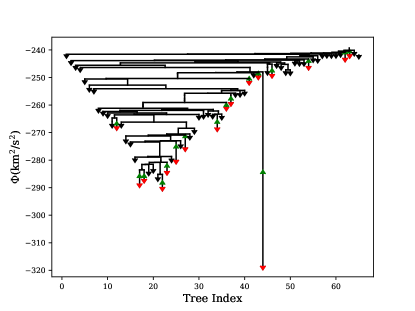
We can use a dendrogram as a graphical representation of the gravitational potential contour tree. Simultaneously, a dendrogram represents the structure of the gravitational potential and shows where HBRs are relative to that structure. We compute a dendrogram so that local minima in the gravitational potential are spaced evenly (“Tree Index”) and ordered so that two objects that intersect are nearby. Then, the intersections can be represented by non-overlapping horizontal lines, and distances in “Tree Index” roughly encode 3-D spatial distances, since intersecting isocontours are obviously in contact with each other. We start with a list of all isocontours on top of the tree with no parents. A complete contour tree should only have one such isocontour containing all points, but it may be desired to terminate the evaluation of the contour tree early. Then, each member of the list is replaced with itself followed by its immediate children, the isocontours that merged to form it. This repeats for each new member of the list and can be performed recursively. Forming this list top-down keeps children together, with only their descendents between them, which ensures that intersections do not overlap. Then, the tree is plotted in reverse, since deeper descendents appear later in the list and need to be plotted first, as the average of their “Tree Index” determines the “Tree Index” of their parents. Local minima are plotted first and given integer “Tree Index,” which evenly spaces them, as desired.

Figure 2: A progression of surface density snapshots from the TIGRESS 2pc (MHD_2pc) simulation at 370, 390, and 410 Myr (from top to bottom) comparing energy-identified objects (left) to density-identified objects (right). Red contours show projections of HBR (left) and $n_{\rm H,min}=100\;{\rm cm}^{-3}$ objects (right). Black contours show HBP (left) and $n_{\mathrm{H}}>10\;{\rm cm}^{-3}$ objects (right).

Figure 3: A representation of the contour tree, or dendrogram, showing objects according to their gravitational potential value ($\Phi$, in units of $(\;{\rm km}\;{\rm s}^{-1})^{2}$) and relative position in the tree. This corresponds to the bottom panels of Figure 2, from the 2pc resolution simulation at 410 Myr. Downward carets show local minima of the gravitational potential, with red carets showing minima hosting HBR. The bases of upward green carets show the maximum $\Phi$ isocontour of each HBR, bound relative to a horizontal black line delineating the maximum $\Phi$ of its HBP. Regions between critical points are represented as vertical black lines, and critical points are horizontal black lines where those regions intersect and merge in this tree diagram.

3 Results

3.1 Structure geography and object dendograms

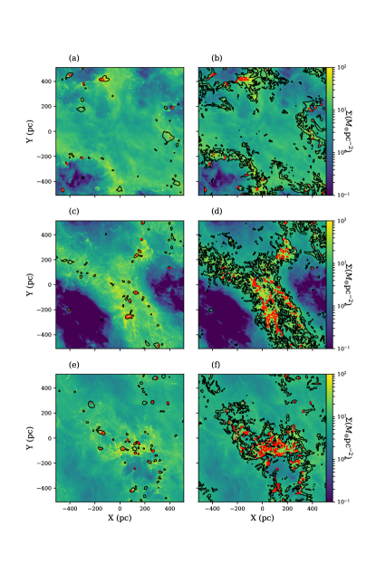
Sample surface density snapshots from the MHD_2pc TIGRESS model can be seen in Figure 2. Also shown, in left-hand panels, is a comparison between HBR and HBP objects, projected onto the horizontal plane. In the right-hand panels, we similarly show projections of objects defined by density thresholds $n_{\rm H,min}=10\;{\rm cm}^{-3}$ and $n_{\rm H,min}=100\;{\rm cm}^{-3}$. This comparison highlights the smoother and more selective nature of energy-identified objects.

A sample dendogram of the HBP and HBR objects identified in Figure 2e is shown in Figure 3. The dendrogram reveals several qualitative properties. For example, ISM turbulence is of the order $v\sim 1-10\;{\rm km}\;{\rm s}^{-1}$, so it is expected that bound material must be found in wells with depths of $\Delta\Phi\sim 1-100\mathrm{km^{2}/s^{2}}$. At a glance, this is apparent in Figure 3. Most local minima, and most of the regions represented by the tree do not host bound regions. The differences between the tops of HBRs and the tops of HBPs, roughly represents the total energy and corresponds to $v\sim 1\;{\rm km}\;{\rm s}^{-1}$.

Furthermore, we can see that the merging criterion described in Section 2.1 usually prefers the smallest scale isocontours at this resolution, corresponding to critical isocontours containing only 1 local minimum. That is, no merging occurs to produce HBR in the snapshot represented by Figure 3, and in general this is rare. A merged HBR would appear as a green upward caret on a vertical line (representing a volume) stemming above (containing) a horizontal line (representing an intersection between isocontours of multiple local minima). Qualitatively, this is because merging adds very little $\Delta\Phi$ for each merge, as evidenced by short vertical lines in Figure 3 corresponding to $v\sim\;{\rm km}\;{\rm s}^{-1}$, but quickly moves to larger length scales and higher velocity dispersion.

Note that Figure 2 (panels e and f) shows that the gas is mostly contained in a single large-scale region, which should result in an overall potential well of the simulation. This is represented in the dendrogram as the overall well shape, except for the large isocontour at (-200 pc, 300 pc) corresponding to index 44. The densest gas and the bound gas in the hierarchy tends to be near the bottom of the overall well of the simulation.

3.2 Gas Distribution and Object Properties

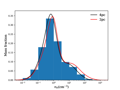
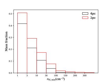
First, we summarize some of the basic properties of the gas in the simulations. In Figure 4 we show the number density distribution in the 4pc and 2pc simulations, taken over all times. We show mass fractions of half-decade bins in number density and normalize the continuous distribution accordingly. In both simulations the mass pdfs are centered near $n_{\mathrm{H}}=1~{}\;{\rm cm}^{-3}$ (mass-weighted mean densities are $n_{\mathrm{H}}=4.84$ and $10.1\;{\rm cm}^{-3}$ for 4pc simulation and 2pc simulation, respectively) with maximum density of $10^{2.5}\;{\rm cm}^{-3}$ in the 4pc simulation and $10^{3}\;{\rm cm}^{-3}$ in the 2pc simulation. The mode of the distribution is at density of $n_{\mathrm{H}}=0.7\;{\rm cm}^{-3}$ and $n_{\mathrm{H}}=0.8\;{\rm cm}^{-3}$ for 4pc simulation and 2pc simulation, respectively. The distribution depends on resolution at high number density due to the criterion for introducing sink particles when collapsing objects become unresolved.

The density distribution is dominated by a roughly log-normal distribution, with a secondary cold dense component. In Figure 5 we show the mass fractions above number density thresholds. In the 2pc simulation, roughly half of the mass is denser than $n_{\mathrm{H}}=1\;{\rm cm}^{-3}$, roughly a tenth of the mass is denser than $30\;{\rm cm}^{-3}$, and a few per cent of the mass is denser than $100\;{\rm cm}^{-3}$. Compared to the lower-resolution model, the 2 pc model has slightly larger mass fractions at higher density.

Figure 4: The hydrogen number density distributions of TIGRESS Solar neighborhood simulations with 2 pc (red) and 4 pc (black) resolution, taken at late times ($t>300$ Myr). Half decade bins are shown for the 4 pc simulation case, showing the fraction of the total mass in each bin.

Figure 5: As in Figure 4 except with cumulative distributions of the hydrogen number density.

Next we describe properties of $n_{\rm H,min}$ objects, using thresholds of $n_{\rm H,min}=$ 10, 30, and $100\;{\rm cm}^{-3}$, and compare them to HBR objects. For the following examination of object properties we only use the 2pc simulation so that objects are better resolved.

Figure 6: Number-weighted (blue, right axis) and mass-weighted (black, left axis) distributions of mass, radius, number density, and free-fall time, for objects defined in the 2 pc resolution simulation. The top two rows show distributions for HBP (Parent) and HBR (Bound) objects, and the bottom two rows show distributions for objects defined by density threshold of $n_{\rm H,min}=$ 10 and $100\;{\rm cm}^{-3}$. The radii are computed from the volume as $R=\sqrt[3]{3V/4\pi{}}$.

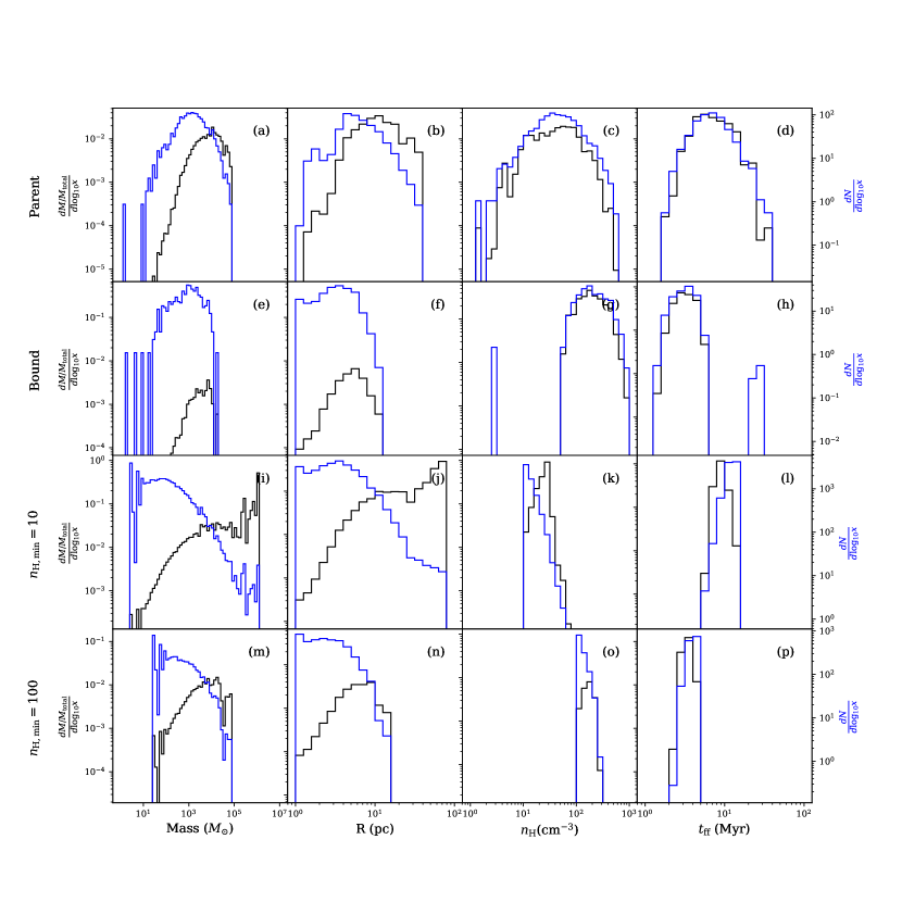
In Figure 6 we present number-weighted and mass-weighted distributions of mass, radius, density, and free-fall time for HBR and HBP objects as well as objects defined by number density thresholds $n_{\rm H,min}=$ 10 and $100\;{\rm cm}^{-3}$. For HBR objects, the typical mass is $10^{3}-10^{4}\;M_{\odot}$, with very few above $10^{4}\;M_{\odot}$. The HBR objects are mostly dense, with $n_{\mathrm{H}}$ a few $100\;{\rm cm}^{-3}$. Hence, it is useful to compare HBR to density objects (both threshold and bin) around $100\;{\rm cm}^{-3}$. The characteristic free-fall times of HBR objects are short ($t_{\mathrm{ff}}\sim 3$ Myr).

Radii of HBR objects are typically several pc, which demonstrates that they are well-resolved with 2pc resolution. We note that a barely resolved 4x4x4 region of cells would have a volume of $8^{3}=512\;{\rm pc}^{3}$. For number densities of 10, 30, and $100\;{\rm cm}^{-3}$, such a region would respectively have masses of 170, 500, and $1700\;M_{\odot}$ assuming $\mu=1.4$. We find very few HBR objects below this lower mass limit set by resolution.

HBP objects have larger sizes and masses than HBR objects, with lower characteristic densities (a few tenths) with free-fall times nearly 10 Myr.

There are a large number of $n_{\rm H,min}$ objects at small masses and radii, since we place no lower cutoff on their size. However, most of the mass is in objects of large mass and radius. For $n_{\rm H,min}=10\;{\rm cm}^{-3}$, typical (in a mass-weighted sense) objects are $10^{5}-10^{6}\;M_{\odot}$ and $\lesssim 100\;{\rm pc}$. For $n_{\rm H,min}=100\;{\rm cm}^{-3}$, typical objects are $10^{4}-10^{5}\;M_{\odot}$ and $\lesssim 10\;{\rm pc}$.

Figure 7: Distributions in virial parameters and mass of various defined objects in the 2pc simulation. Left panels show HBRs, and central and right panels show $n_{\rm H,min}=10,30$, and $100\;{\rm cm}^{-3}$ objects. In the top row (panels a, b, c, and d), only kinetic energy is considered for $\alpha_{v}$ (Equation 8). In the bottom row (panels e, f, g, h) $\alpha_{v,\mathrm{total}}$ considers kinetic, thermal, and magnetic energy (Equation 9). Dashed horizontal lines delineate $\alpha_{v}=2$ or $\alpha_{\rm v,total}=2$, corresponding to $E_{\rm k}=E_{\rm g}$ in top panels and $E_{\rm k}+E_{\rm B}+E_{\rm th}=E_{\rm g}$ in bottom panels. Vertical lines represent the minimum mass estimate from Equation 26. Contours show the distribution of $n_{\rm H,min}$-objects whose mass has less than one per cent overlap with HBR. Scatter points are individual $n_{\rm H,min}$-objects whose color reflects their mass fraction overlap with HBR. Truly bound objects (red points) with order unity overlap with HBR tend to be low mass (around $10^{3}\;M_{\odot}$) with virial parameters $\alpha_{v}\lesssim 2$. Especially at high masses, many apparently “bound” objects based on $\alpha_{v}<2$ are not in fact HBR-bound (i.e. they are colored blue-green-yellow). Additionally, many $\alpha_{v}>2$ and $\alpha_{v,total}>2$ objects at low and moderate density have significant HBR overlap (red). These results show that “observed” virial parameter is not a good indication of true gravitational binding.

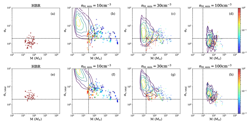
Figure 7 shows the distribution of virial parameters and masses for HBR and $n_{\rm H,min}$ objects, via contours and scatter plots. For scatter plots of individual $n_{\rm H,min}$ objects, the color of each point indicates the fraction of its mass that is bound, based on overlap with HBR objects. We find that very few $n_{\rm H,min}$ objects at the low mass end ($<10^{3}\;M_{\odot}$) have overlap with HBR, even if their kinetic virial parameter $\alpha_{v}<2$. $n_{\rm H,min}$ objects with negligible (less than one per cent) overlap with HBR are represented by contours enclosing $20\%$, $40\%$, $60\%$, $80\%$, and $90\%$ of the objects.

The depth of a well behaves as $GM/R\sim G\rho{}R^{2}$. At constant density, only a sufficiently large object will have a well deep enough to bind material. A rough estimate comparing $GM/R>v^{2}$ with $M=(4\pi{}/3)\rho{}R^{3}$ yields a minimum mass that follows

$$M^{2}>\frac{v^{6}}{\frac{4\pi}{3}G^{3}\rho{}}.$$ (26)

For $v=1\;{\rm km}\;{\rm s}^{-1}$ and $n_{\rm H,min}=30\;{\rm cm}^{-3}$, this minimum mass is $2\times 10^{3}\;M_{\odot}$. The $n_{\rm H,min}=10\;{\rm cm}^{-3}$ and $n_{\rm H,min}=30\;{\rm cm}^{-3}$ objects overlapping HBR lie above their respective minimum mass (for $v=1\;{\rm km}\;{\rm s}^{-1}$), whereas the $n_{\rm H,min}=100\;{\rm cm}^{-3}$ objects all lie above the resolution minimum mass (which is greater than the well minimum mass).

For objects of mass $\sim 10^{3.5}-10^{4}\;M_{\odot}$, those at the lower range of $\alpha_{v}$ and $\alpha_{v,total}$ have the largest fraction of bound gas (i.e. red colored points), which is consistent with general expectations. However, the actual values of $\alpha_{v}$ and $\alpha_{v,total}$ in the objects with $>50\%$ HBR-overlap cover a wide range from $\alpha_{v}\sim 0.6-6$, generally decreasing at higher density. This shows that the “observed” virial parameter is not a very accurate quantitative measure of gravitational boundedness.

Furthermore, Figure 7 shows that unlike low-mass ($\sim 10^{3.5}-10^{4}\;M_{\odot}$) $n_{\rm H,min}$ objects with $\alpha_{v}\lesssim 2$ which are generally bound, $n_{\rm H,min}$ objects at the high mass end ($>10^{4.5}\;M_{\odot}$) have very little overlap with HBRs even at low virial parameter ($\alpha_{v}<2$). That is, high mass objects ($10^{6}\;M_{\odot}$) can appear bound based on simple criteria using their mass, size, and velocity dispersion (Equation 8), but in reality this is not consistent with full gravitational potential structure. This is in part due to tidal fields preferentially unbinding larger-scale objects, and in part due to substructure. Substructure within a $n_{\rm H,min}$ object manifests itself as multiple separate HBR objects which comprise a small fraction of the mass because most of the mass lies in between HBRs.

In summary, we find that overdense objects with $\alpha_{v}\lesssim 2$ are truly bound only if their masses are low; high-mass objects are generally unbound even when a simple estimate suggests otherwise.

Figure 8: The fraction of mass in objects defined by density thresholds that is also within HBR objects; this is equivalent to the conditional probability $P(\rm bound|\rm dense)$, in the 2pc simulation. This increases with density $n_{\rm H,min}$, but even at high densities (100 $\;{\rm cm}^{-3}$) only $\sim 10\%$ of the mass is bound.

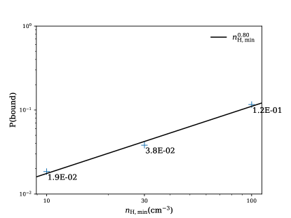
In Figure 8 we show the HBR fraction of the mass above number density thresholds $n_{\rm H,min}=10$, $30$, and $100\;{\rm cm}^{-3}$, representing the probability of gas being bound given that it is dense. This fraction is only a few per cent for $n_{\rm H,min}=10\;{\rm cm}^{-3}$ and $30\;{\rm cm}^{-3}$, increasing to $10\%$ for $n_{\rm H,min}=100\;{\rm cm}^{-3}$. The fraction roughly follows the power law $n_{\rm H,min}^{0.80}$. Since HBR mass tends to be dense, each density threshold should contain nearly all the HBR mass. Thus, the overlap fraction should roughly follow the reciprocal of the threshold distribution as shown in Figure 5 (for the 2pc simulation). The threshold distribution at these number densities follows $n_{\rm H,min}^{-0.87}$, whose reciprocal has a similar slope as expected. Although the $n_{\rm H,min}=100\;{\rm cm}^{-3}$ threshold is within an order of magnitude of the maximum density in the simulation, and the Larson-Penston density is one of the criteria for star particle formation, we do not find strong evidence for a critical density for boundedness within the range $n_{\mathrm{H}}=10-100\;{\rm cm}^{-3}$.

Figure 9: The linewidth-size ($\sigma_{3D}$ and radius from $V=(4\pi/3)R^{3}$ for object volume $V$) relationship of various objects (number density threshold, HBR, HBP) from the 2 pc TIGRESS solar neighborhood simulation. In panels a-e, contours show the full distribution and the blue line shows the median value of radius bins. The contours contain $20\%$, $40\%$, $60\%$, $80\%,$ and $90\%$ of the objects. For reference, the black dashed line represents $\sigma\propto R^{1/2}$ with normalization set by the measured velocity dispersion of $T<2\times{}10^{4}K$ gas for $R$ equal to the measured scale height in the simulation. In panels a-c, the black dotted line represents spheres at the threshold density with equal kinetic and potential energy ($\sigma\propto Rn_{\rm H,min}^{1/2}$). The solid black line is $\sigma\propto R^{1/2}$ with normalization similar to that of Milky Way GMCs $\sigma_{3D}=\sqrt{3}\times 0.9\;{\rm km}\;{\rm s}^{-1}(R/\;{\rm pc})^{1/2}$ (Heyer & Dame, 2015). The median relations of all object types are stacked in the bottom-right panel.

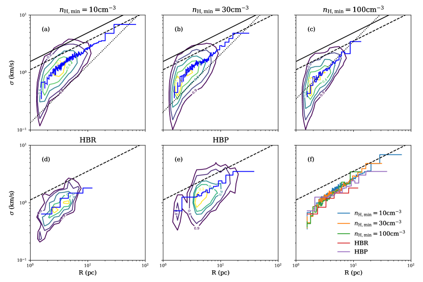
We show in Figure 9 the linewidth-size relationships of $n_{\mathrm{H}}$-threshold, HBR, and HBP objects. Here, the linewidth for an object is defined as $\sqrt{2E_{\rm k}/M}$ where $M$ is the mass and $E_{\rm k}$ is the kinetic energy in the object’s center of mass frame. The size is computed from object volume $V$ taking $V=(4\pi/3)R^{3}$.

Panels a-e of the figure include both contours of each distribution and median relationships, with bins for the latter chosen to each contain 100 objects, except for the final bin. We also include several reference lines with slopes $\sigma\propto R^{1/2}$ and $R$ for comparison. $n_{\rm H,min}$ objects and HBRs have linewidth-size relationships that are somewhat steeper than $\sigma\propto R^{1/2}$, which is what would be expected if all the objects simply sampled from the same power spectrum of highly compressible ISM turbulence with an outer scale much larger than typical object sizes. The objects with the closest linewidth-size relation to $\sigma\propto R^{1/2}$ are HBPs, which are formed by isocontours of the gravitational potential. While there are detailed differences among the median linewidth-size relationships for different object categories, Figure 9f shows that the median relationships are in fact quite similar across all categories.

For $n_{\rm H,min}$-objects, in each panel of Figure 9 we also include the line corresponding to a spherical object with density equal to the threshold density and kinetic energy equal to the potential energy, which has slope $\sigma\propto Rn_{\rm H,min}^{1/2}$. Moving to higher $n_{\rm H,min}$ shifts the $\sigma\propto R$ line from self-gravitation upward since $\sigma_{3D}=(\rho G8\pi/5)^{1/2}R$.

For density threshold $n_{\rm H,min}=10,30\;{\rm cm}^{-3}$, most objects lie above the marginally self-gravitating locus. For the $n_{\rm H,min}=100\;{\rm cm}^{-3}$ threshold, the median relationship follows the marginally-bound relation quite well. These results are consistent with the results for the distributions of $\alpha_{v}$ shown in Figure 7, which shows that the typical $\alpha_{v}$ decreases with $n_{\mathrm{H}}$ threshold. We again emphasize that even with order-unity $\alpha_{v}$, most of the material in objects above a density threshold $n_{\rm H,min}=100\;{\rm cm}^{-3}$ is not part of bound regions.

3.3 Time Series

We now turn to the results of our time series analysis, based on methods described in Section 2.3. Since a large number of snapshots is necessary for this analysis, we primarily use the 4pc simulation, which was run for a longer time.

Figure 10: Time series of mass fractions for various categories of objects and density bins, as labeled, for the 4 pc resolution Solar neighborhood simulation. HBRs are bound objects and HBPs are their parents; see text in Section 2.1 for explanation of treatment of surface terms in HBR$\pm$1. The quasi-periodic variations in the $n_{\mathrm{H}}$ bin time series reflect the natural 50 Myr vertical oscillation timescale in the galactic potential.

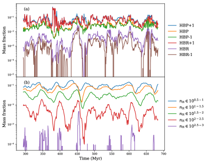
In Figure 10 we show how the mass fractions of different categories of material evolve over time. The top panel shows HBR and HBP material as well as HBR$\pm$1, where the latter allows for surface terms to help confine or else disperse material, and HBP$\pm$1 are the “parents” of HBR$\pm$1 objects (see Section 2.1 for details of definitions). HBP+1 and HBR+1 include more mass and HBP-1 and HBR-1 include less mass, as described in Section 2.1. The bottom panel shows the mass fractions of material in half-decade number density bins. Overall, the amplitude of fluctuations increases for categories with lower mean mass fractions. In addition, upward fluctuations are successively delayed in time for increasing $n_{\mathrm{H}}$ bins; we discuss this effect further below.

Roughly $10\%$ of the mass is in low density bins and in HBR+1/HBP+1 objects. HBR+1 and HBP+1 objects effectively subtract the surface value of kinetic, thermal, and magnetic energy from each cell in the object, such that low density material in the shallower regions of a potential well is considered bound and the object mass is higher than if surface terms were neglected. The HBR+1 mass is close to the HBP+1 mass because nearly all the material within an isocontour is considered bound. A few per cent of the mass is within HBP-1 and HBP objects, which have relatively similar mass histories. Only of order $10^{-3}$ of all the material in the simulation is in HBR and HBR-1 objects. Relative to HBR, HBR-1 objects have slightly less mass because the surface energy terms are added to each cell, reducing the amount of material that is considered bound.

Figure 11: Comparison between star formation rate (SFR) and mass divided by free-fall time $M/t_{\mathrm{ff}}{}$ of various gas populations from $t=300-700$ Myr in the 4 pc resolution Solar neighborhood simulation. The SFR shown is smoothed over 5 Myr and normalized to its time-average value. The $M/t_{\mathrm{ff}}{}$ time series are also normalized relative to their time-averaged values. Individual panels compare (a) surface density thresholds, (b) number density thresholds, (c) number density bins, and (d) HBP and HBR. In all cases the denser, more restrictive definition leads to a qualitatively better match between SFR and $M/t_{\mathrm{ff}}{}$.

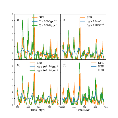
It is interesting to compare the SFR history with the evolution of $M/t_{\mathrm{ff}}$ at lower and higher gas surface density $\Sigma$, lower and higher density $n_{\mathrm{H}}$, and for less and more bound objects. By comparing time series in Figure 11, it is evident that more restrictive definitions have an improved correlation with $\mathrm{SFR}$. This holds for increasing threshold $\Sigma$, increasing $n_{\mathrm{H}}$ threshold, increasing $n_{\mathrm{H}}$ bins, and increasing boundedness from HBP to HBR. Intriguingly, Figure 11b,c demonstrate that simple density criteria (high density threshold or bin) yield better correlation with SFR than the more complex criteria based on total energy in the full gravitational potential landscape that go into the definition of HBR, shown in Figure 11d. The visual impressions of these histories already suggest that gravitational binding is not a guarantee that star formation will be successful; we return to this quantitatively below.

Figure 12: Comparison between SFR and $M/t_{\mathrm{ff}}{}$ as in Figure 11 for half-decade number density bins Here $M/t_{\mathrm{ff}}{}$ is normalized by a factor of $\epsilon_{\mathrm{ff}}{}/\left\langle{\mathrm{SFR}}\right\rangle$, where $\epsilon_{\mathrm{ff}}{}$ is the result of the simple linear regression (Equation 11). The inferred delay time $t_{d}$ is used to offset the time series, which is labeled as “delayed” for each number density bin. It is clear that the correlation between SFR and $M/t_{\mathrm{ff}}{}$ improves and $t_{d}$ decreases as density increases.

Figure 13: The delay time $t_{d}$ vs. lower density edge of some of the half-decade density bins shown in Figure 12. Lines for $t_{\mathrm{ff}}{}=[3\pi/(32G\mu n_{\mathrm{H}})]^{1/2}$ are computed using the lower and upper number density edge, respectively resulting in a maximum and minimum free-fall time. For denser bins, the delay time roughly follows the minimum free-fall time.

Figure 14: Comparison of $\mathrm{SFR}$ and $\epsilon_{\rm ff}M/t_{\mathrm{ff}}$ as in Figure 12 for surface density thresholds ($\Sigma=$ 10 and $30\;M_{\odot}\;{\rm pc}^{-2}$), number density thresholds ($n_{\rm H,min}=$ 10, 30, and $100\;{\rm cm}^{-3}$), and HBR (bound) objects, showing only the delayed time series.

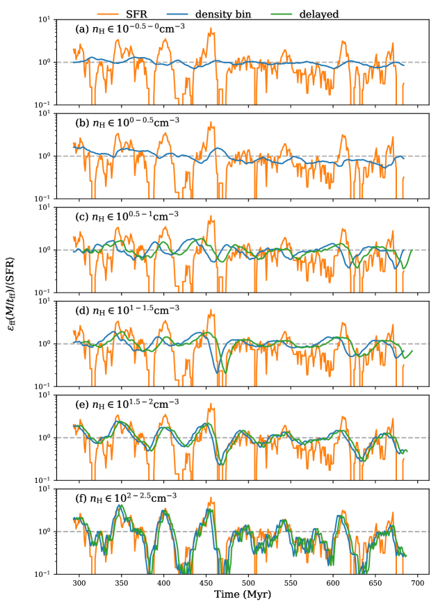
As described in Section 2.3, we can apply linear regression to obtain both the optimal time delay to match the shape of each $M/t_{\mathrm{ff}}$ time series to the SFR, and the corresponding normalization amplitude $\epsilon_{\mathrm{ff}}$ that measures the best-fit star formation efficiency per free-fall time. Figure 12 shows the result of applying this linear regression, demonstrating that higher $n_{\mathrm{H}}$ bins correlate more strongly to SFR, with a smaller time delay, compared to lower $n_{\mathrm{H}}$ bins. Even at low $n_{\mathrm{H}}=10^{0.5}\;{\rm cm}^{-3}$ some correlation is apparent, but not for lower densities. Thus, while the amount of gas in low density bins ($n_{\mathrm{H}}=10^{-0.5}-10^{0.5}$) comprising the bulk of ISM mass (see Figure 4) varies in time due to large-scale vertical and horizontal oscillations that produce ISM compressions and rarefactions, these variations do not appear to directly induce star formation.

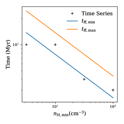
In Figure 13 we show that the time delay inferred from the fit is comparable to the free-fall time associated with the $n_{\mathrm{H}}$ bin upper edge, $t_{\mathrm{ff,min}}=[3\pi/(32G\mu n_{\mathrm{H,max}})]^{1/2}$, with $n_{\mathrm{H,max}}=10^{0.5}n_{\mathrm{H,min}}$. This is consistent with the idea that a variation in mass or $M/t_{\mathrm{ff}}$ at a given density can only lead to a variation in SFR after the gas is able to dynamically respond; the minimum response time is the free-fall collapse time at that density, and this indeed appears to be the defining timescale, even though the efficiency of collapse is less than unity.

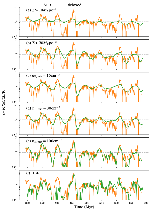
In Figure 14 we compare histories of star formation with the time series of $\epsilon_{\rm ff}M/t_{\mathrm{ff}}$ for best-fit time delay and $\epsilon_{\rm ff}$ for material defined by surface density threshold, number density threshold, and HBR objects. For surface density and number density, correlation with SFR improves with a higher threshold. This correlation is visually similar for $\Sigma>30\;M_{\odot}\;{\rm pc^{-2}}$, $n_{\mathrm{H}}>10,30\;{\rm cm}^{-3}$. Although HBR and $n_{\mathrm{H}}>100\;{\rm cm}^{-3}$ both follow $\mathrm{SFR}$ quite closely (and in particular follow lows much better than predictions based on lower density thresholds), in fact the mass of HBR gas provides a slightly worse prediction of $\mathrm{SFR}$ than the mass of gas at $n_{\mathrm{H}}>100\;{\rm cm}^{-3}$. We quantify this in the next subsection.

3.4 Star Formation Efficiency

Figure 15: Inferred $\epsilon_{\mathrm{ff}}{}$ (a, b, e, f) and RMS error $\sigma_{\Delta\mathrm{SFR}/\langle\mathrm{SFR}\rangle}$ (c, d , g, h) based on time series of SFR compared to time series of $M/t_{\mathrm{ff}}$ for selected subsets of the gas, as labeled. Gas selection criteria include density ($n_{\mathrm{H}}$) thresholds and bins, surface density ($\Sigma$) thresholds, bound objects (HBR) and their parents (HBP), overlaps between density and HBR objects ($j$), combined density and $\alpha_{v}<2$ criteria ($v$); see text for details. In each panel, results from 4pc are shown as darker points with 2pc ($\epsilon_{\mathrm{ff}}$ only)shown as lighter points. Errorbars from Equation 25 are not shown but would lie within markers, decreasing with the number of time snapshots used.

In this section, we present results on our inference for efficiency per free-fall time $\epsilon_{\mathrm{ff}}$ for various subsets of gas, based on application of the methods of Section 2.3. We are interested in both the measures of $\epsilon_{\mathrm{ff}}$ and how they depend on the criteria for defining a subset of the gas, and quantitative assessment of the relative performance for predicting SFR. We include results from both the 4pc simulation time series, which based on its larger number of snapshots is advantageous in terms of sample size, and the 2pc simulation, which allows us to test whether our results are converged with respect to numerical resolution.

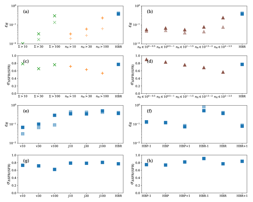
Figure 15 shows for several different categories of objects the values for $\epsilon_{\mathrm{ff}}$ and for $\sigma_{\Delta\mathrm{SFR}/\langle\mathrm{SFR}\rangle}$ based on linear regression. The top two rows show results for gas subsets defined by $\Sigma$ and $n_{\mathrm{H}}$ thresholds and by $n_{\mathrm{H}}$ bins, also comparing to HBR results. For both $\Sigma$ and $n_{\mathrm{H}}$ thresholds (Figure 15a,c), the total mass decreases faster than the free-fall time as the threshold increases. As a result, ${M/t_{\mathrm{ff}}}$ decreases at increasing density, leading to an increase in $\epsilon_{\mathrm{ff}}$ with threshold level. At the same time, $\sigma_{\Delta\mathrm{SFR}/\langle\mathrm{SFR}\rangle}$ mostly decreases with increasing threshold, implying better correlation of denser gas with SFR; this is consistent with the visual impression from previous plots. When we consider subsets of gas in density bins (Figure 15b,d), $\epsilon_{\mathrm{ff}}$ increases and $\sigma_{\Delta\mathrm{SFR}/\langle\mathrm{SFR}\rangle}$ decreases at higher densities $n_{\mathrm{H}}$. However, at $n_{\mathrm{H}}<10^{1.5}\;{\rm cm}^{-3}$, $\epsilon_{\mathrm{ff}}$ is roughly flat at roughly $0.06$. The value $\epsilon_{\mathrm{ff}}\sim 0.01$ for $\Sigma>10\;M_{\odot}\;{\rm pc^{-2}}$ represents the mean efficiency for the bulk of the material in the simulation.

Interestingly, while the values of $\epsilon_{\mathrm{ff}}$ for high density thresholds are similar to the value of $\epsilon_{\mathrm{ff}}$ for gas in HBR (a few tenths), the value of $\sigma_{\Delta\mathrm{SFR}/\langle\mathrm{SFR}\rangle}$ is lower for density thresholds than for HBR gas. While HBR gas is mostly quite dense, this says that the additional criteria of requiring that every parcel of gas is bound within an HBR does not lead to better agreement in the histories.

Looking at HBP and HBR variants in Figure 15f,g, higher mass variants (all HBP, and HBR+1) have lower $\epsilon_{\mathrm{ff}}$ ($\sim 0.1$). HBR has $\epsilon_{\mathrm{ff}}\approx 0.4$ and HBR-1 has $\epsilon_{\mathrm{ff}}\approx 0.6$: in both cases the efficiency is nearly order unity, as might be expected of truly collapsing objects. However, we cannot distinguish between the case that each bound object takes a total time $t_{\mathrm{ff}}/\epsilon_{\mathrm{ff}}$ to collapse, vs. the case that the probability of each bound object being dispersed is $1-\epsilon_{\mathrm{ff}}$ and the collapse timescale for surviving objects is $t_{\mathrm{ff}}$. The variants of HBR and HBP have a similar correlation to SFR, but HBR and HBP have slightly lower $\sigma_{\Delta\mathrm{SFR}/\langle\mathrm{SFR}\rangle}$. It is interesting that isocontours alone (HBP) provide a reasonable correlation to SFR, and that varying treatment of surface terms has little effect.

We can also consider combined criteria and test the correlation with SFR. In Figure 15e,g, we show results for “$j$” time series, consisting of material that exceeds certain density thresholds and also overlaps with HBRs, and for “$v$” time series, material in $n_{\rm H,min}$ objects that also satisfy $\alpha_{v}<2$ (kinetic energy only, excluding thermal and magnetic, in the virial parameter). The $v$ series has similar results to $n_{\rm H,min}$ objects themselves, but with slightly greater $\epsilon_{\mathrm{ff}}$ and comparable $\sigma_{\Delta\mathrm{SFR}/\langle\mathrm{SFR}\rangle}$. Whereas $\epsilon_{\mathrm{ff}}$ for $n_{\mathrm{H}}>10\;{\rm cm}^{-3}$ doubles when considering $\alpha_{v}$ in the $v$ series, it is only higher by $30\%$ in the $n_{\mathrm{H}}>100\;{\rm pc}$ case. Considering the virial parameter mainly affects lower density gas.

The “$j$” series over material overlapping between HBR and $n_{\rm H,min}$ objects is mostly similar to HBR because most HBR mass also satisfies $n_{\mathrm{H}}\sim 100\;{\rm cm}^{-3}$. The exception is $n_{\mathrm{H}}>100\;{\rm pc}$ in the 4pc case because $100\;{\rm cm}^{-3}$ is close to the maximum density of the simulation.

Note that although $\epsilon_{\mathrm{ff}}$ for surface and $n_{\rm H,min}$ objects are resolution dependent (4pc and 2pc points differ), the values of $\epsilon_{\mathrm{ff}}$ for low- and moderate-$n_{\mathrm{H}}$ bins are resolution independent. Thus, differences in $n_{\rm H,min}$ objects are due to the lack of gas in high density bins for lower resolution simulations. Unlike the high-$n_{\mathrm{H}}$ series, the HBR and HBP series (and their variants) have essentially the same values of $\epsilon_{\mathrm{ff}}$ at 4pc and 2pc resolution. The difference in $\sigma_{\Delta\mathrm{SFR}/\langle\mathrm{SFR}\rangle}$ with resolution primarily reflects the different number of snapshots available at each resolution. Whereas multiple cycles of star formation are available in the 4pc simulation, only 70 Myr of snapshots are available from the 2pc simulation. Therefore, we do not draw any conclusions from the 2pc values of $\sigma_{\Delta\mathrm{SFR}/\langle\mathrm{SFR}\rangle}$ and do not show those values in Figure 15.

Figure 16: A comparison of the distribution of $\Delta\mathrm{SFR}/\langle\mathrm{SFR}\rangle$ (see Equation 13), the difference between actual and predicted SFR using different categories of gas, based on (a)-(b) gas surface density threshold, (c)-(e) number density threshold, and (f) HBR objects, corresponding to the time series shown in Figure 14. The mean error is shown as a blue vertical line, and quartiles are shown in black lines (median in solid, 25 and 75 dashed).

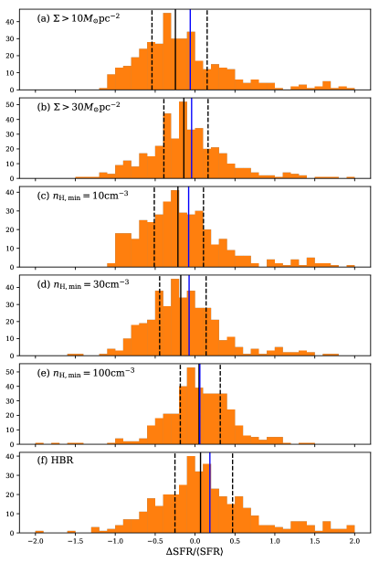
In Figure 16 we illustrate how correlation changes for different gas selection criterion in further detail by providing histograms of the error $\Delta\mathrm{SFR}/\langle\mathrm{SFR}\rangle$ (Equation 13), where a positive error means that the simulated star formation rate is higher than the model star formation rate based on $M/t_{\mathrm{ff}}$ for a single snapshot. For less restrictive selection criteria, such as lower $n_{\mathrm{H}}$ or $\Sigma$, the mean and median in the distributions shift to the left, indicating that the predicted $\epsilon_{\mathrm{ff}}M/t_{\mathrm{ff}}$ exceeds the actual SFR. This is clearly evident in Figure 14: for low density thresholds, there is little predicted variation in the SFR about the mean, whereas the true SF history is mostly below the mean level, with some sharp peaks. Figure 16 also shows that worse correlation at lower $n_{\mathrm{H}}$ or $\Sigma$ threshold is associated with a larger number of snapshots wherein $\Delta\mathrm{SFR}/\langle\mathrm{SFR}\rangle\sim-0.5-1$ and $\Delta\mathrm{SFR}/\langle\mathrm{SFR}\rangle>1$. Again, this is evident in the missed “long valleys” and “sharp peaks” for the prediction based on $\epsilon_{\mathrm{ff}}M/t_{\mathrm{ff}}$ in the $\Sigma>10\;M_{\odot}\;{\rm pc^{-2}}$, $n_{\mathrm{H}}>10\;{\rm cm}^{-3}$ cases in Figure 14. Since missing sharp peaks occurs during periods of high SFR, considering an alternative version of Equation 14 by weighting by $\mathrm{SFR}(t_{i})$ would amplify the improvement of correlation with increasing density. Figure 16e,f also quantifies the visual impression from Figure 14 that the restriction that gas be bound (HBR) does not offer better predictive power for $\mathrm{SFR}$ compared to a simple high density threshold. In particular, the HBR prediction misses a peak at $t\sim 400$Myr, which accounts for the positive error tail in $\Delta\mathrm{SFR}$ compared to $n_{\mathrm{H}}>100\;{\rm cm}^{-3}$.

Counterintuitive to the immediate visual impression from Figure 14, HBR has larger $\sigma_{\Delta\mathrm{SFR}/\langle\mathrm{SFR}\rangle}$ than even the $n_{\mathrm{H}}>10\;{\rm cm}^{-3}$ and $n_{\mathrm{H}}>30\;{\rm cm}^{-3}$ for the 4pc model, although for the 2pc model HBR performs better. The primary reason for this is the overall much larger range of predicted $\mathrm{SFR}$ from HBR; since this has high peaks that can be slightly offset from the peaks in the true $\mathrm{SFR}$, this leads to a broader distribution of errors in Figure 16. Another reason is that HBR can be too selective, where there are snapshots with high SFR but insufficient corresponding HBR gas mass.

3.4.1 Dependence on virial parameter

Figure 17: Comparison of inferred model parameters and goodness of fit for three models of the dependence of SFR on $\alpha_{v}$ as described in Section 2.3.1. Results are shown for model with no $\alpha_{v}$ dependence (blue points), model with exponential dependence on $\alpha_{v}^{1/2}$ (orange points; Equation 17), and model with an $\alpha_{v}$ cutoff (green points; Equation 18). Points and bars represent the mean (Equation 24) and standard deviation (from Equation 25) of marginalized distributions for time delay $t_{\mathrm{delay}}$ (in Myr), efficiency $\epsilon_{\mathrm{ff}}$, slope $\beta$ for the exponential model, and cutoff $\alpha_{v}$. Standard deviations of normalized $\mathrm{SFR}$ errors $\sigma_{\Delta\mathrm{SFR}/\langle\mathrm{SFR}\rangle}$ (inferred $\sigma$ in Equation 20) are shown for all models. Reference values $\beta=1.6$ and $\alpha_{v}=2$ are shown with horizontal dashed lines. Columns left to right use thresholds $n_{\mathrm{H}}>10$, $30$, and $100\;{\rm cm}^{-3}$, and energy-based criteria (HBR) to define objects.

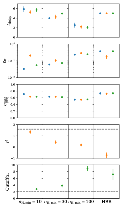
As discussed in Section 2.3.1, we can apply Bayesian inference to our time series to evaluate parameters and explore the relative goodness of fit for different models that have been proposed for the dependence of star formation on the virial parameter. In our tests, we separately examine objects defined by number density thresholds with $n_{\mathrm{H,min}}=10,30$, and $100\;{\rm cm}^{-3}$, as well as HBR objects.

Figure 17 presents the results of our analyses. From left to right, panels show results for objects defined by different density thresholds and by the HBR criterion. Each row gives values of parameters obtained for the three models under consideration: constant $\epsilon_{\mathrm{ff}}$ (blue points, equivalent to the results presented in Figure 15), an exponential dependence on $\alpha_{v}^{1/2}$ (orange points, generalizing Padoan et al. 2012), and a cutoff in $\alpha_{v}$ (green points). The plotted value of $\epsilon_{\mathrm{ff}}$ represents $\epsilon_{\rm ff,0}$ for the exponential and cutoff models.

For all models, from lower density to higher density thresholds the inferred time delay decreases, consistent with Figure 12. At the same time, the inferred $\epsilon_{\mathrm{ff}}$ increases with $n_{\mathrm{H}}$ for both the constant-$\epsilon_{\mathrm{ff}}$ and the virial-cutoff models. The inferred $\epsilon_{\rm ff,0}$ does not monotonically vary with $n_{\mathrm{H}}$ for the exponential model. Going from $n_{\mathrm{H}}>30$ to $n_{\mathrm{H}}>100$, the RMS error $\sigma_{\Delta\mathrm{SFR}/\langle\mathrm{SFR}\rangle}$ decreases for both the exponential and cutoff model, similar to what was shown previously for the model with no $\alpha_{v}$ dependence. Based on RMS error levels for any given gas selection criterion, there is generally no significant preference for the $\alpha_{v}$-dependent models for $\mathrm{SFR}$ compared to the $\alpha_{v}$-independent model. This can be understood considering the inexact correspondence between apparent $\alpha_{v}$ and true boundedness, and the previously-discussed limitations of boundedness as a detailed predictor of the $\mathrm{SFR}$. The exception is the lower-density $n_{\mathrm{H}}>10$ object class, in which both models that account for the virial parameter perform better than the constant-$\epsilon_{\mathrm{ff}}$ model (see further discussion below).

For the exponential model, only the low density threshold case shows a similar slope $\beta\approx 1.6$ to that found by Padoan et al. 2012; at high density $\beta\sim 0$ is preferred, which is equivalent to constant $\epsilon_{\mathrm{ff}}$. This is consistent with expectations, considering the differences between the types of simulations of Padoan et al. 2012 vs. the current models and analysis. In Padoan et al. 2012, the comparison was between global SFRs for small-box simulations of cold gas in which turbulence was driven to different levels. This is most similar to our selection of objects with $n_{\mathrm{H}}>10\;{\rm cm}^{-3}$, and then assigning a relative probability of SF depending on level of the virial parameter (which has a large variation at low density, with only the lower $\alpha_{v}$ objects being massive enough to host star formation, as shown in Figure 7). When we instead select objects that are already quite overdense compared to the average, the range of virial parameters is smaller (as seen in Figure 7) so there is little “leverage.”

For a low density threshold $n_{\mathrm{H}}>10\;{\rm cm}^{-3}$, the $\alpha_{v}$ cutoff model prefers $\alpha_{v}\approx 2$, for similar reasons to the higher preferred $\beta$ in the exponential model. However, at $n_{\mathrm{H}}>30$ and $n_{\mathrm{H}}>100$, the inferred cutoff $\alpha_{v}$ values are larger, demonstrating that the density threshold itself provides a good correlation with the SFR and that removing high $\alpha_{v}$ material is not preferred. Energy-selected HBR objects also do not benefit from a virial parameter cutoff.

4 Conclusion

4.1 Summary

In this work, we have applied structure-finding techniques to TIGRESS simulations of the star-forming ISM, and characterized the properties of the objects we identify. In addition, we have investigated families of relationships between the SFR and material that could be considered “eligible” for star formation, by being part of a subset of the gas with defined properties. For the latter, we consider both collections of objects and more general gas subsets.

Our primary comparison of structures is between those defined based on density or surface density (bins or thresholds) and those that are defined based on the gravitational potential (also considering kinetic, thermal, and magnetic energy). The former is more analogous to the definitions of ISM structure typically used in observations (where boundaries are often defined by observed intensity), whereas the latter more directly connects to dynamics. The definitions and techniques used to identify structures are described in Section 2.1 and 2.2.

For both material defined by density selection criteria and material defined by energy selection criteria, we compare time series of $M/t_{\mathrm{ff}}$ to the SFR history. We use these comparisons to fit for time delays ($t_{d}$) and efficiencies per free-fall time ($\epsilon_{\mathrm{ff}}$). In addition, we apply Bayesian inference to compare three different models for star formation with different dependence on the virial parameter. Techniques are described in Section 2.3 and 2.3.1.

Key results are as follows:

1. Object properties: Basic statistics (mass, size, density, free-fall time) of HBRs (bound objects) and HBPs (their parents) are compared to statistics of $n_{\rm H,min}$ objects defined by density contours in Figure 6. Typical masses of HBRs are $\sim 10^{3}-10^{4}M_{\odot}$, with $n_{\mathrm{H}}\sim 100\;{\rm cm}^{-3}$. HBPs have slightly lower density and masses that extend up to $\sim 10^{5}M_{\odot}$. Thus, bound objects are dense. Most of the mass of $n_{\rm H,min}$ objects is in large structures: typical values are $R\sim 30-100\;{\rm pc}$ and $M\sim 10^{5}-10^{6}\;M_{\odot}$ for $n_{\rm H,min}=10\;{\rm cm}^{-3}$, and $R\sim 10\;{\rm pc}$ and $M\sim 10^{4}\;M_{\odot}$ for $n_{\rm H,min}=100\;{\rm cm}^{-3}$. Not all dense objects are bound (see below).

2. Virial parameters and boundedness: Figure 7 shows the distribution of values of the virial parameter $\alpha_{v}$ most commonly used in observations, which compares kinetic energy with gravitational energy, assuming an isolated sphere with the same mass and volume to compute $E_{\rm g}$ (Equation 8). Figure 7 also shows results for a variant $\alpha_{\rm v,tot}$ that includes thermal and magnetic energy (Equation 9). Because magnetic and kinetic energy are comparable, we find that neglect of magnetic energy in estimating the virial parameter is not justified. Interestingly, while HBR objects are defined based on bound material, they have a range of values for “observed” $\alpha_{v}\sim 0.5-5$ and $\alpha_{\rm v,total}\sim 2-7$. Figure 7 also depicts the fraction of gas in each $n_{\mathrm{H}}$-defined object that is truly bound when considering the full gravitational potential. Many objects that appear bound based on $\alpha_{v}$ in fact contain only a small fraction of bound gas; this is especially an issue at high mass $M\sim 10^{4}-10^{6}M_{\odot}$. Massive, moderate-density objects exist but they are not bound by gravitational wells even when $\alpha_{v}<2$ (Figure 7b,c). The probability of gas being bound increases with $n_{\rm H,min}$ (Figure 8).

3. Linewidth-size relations: Figure 9 shows that the median linewidth-size relation for low-$n_{\rm H,min}$ structures is shallower than and lies above the $\sigma\propto R$ relation for bound objects with fixed density, but is fairly close to the mean $\sigma\propto R^{1/2}$ relation expected for supersonic turbulent gas with outer scale exceeding the cloud scale. At high $n_{\rm H,min}$, the median linewidth does follow the $\alpha_{v}=2$ linewidth-size relation $\sigma_{3D}\approx(\rho G8\pi/5)^{1/2}R$ for $\rho=\mu n_{\rm H,min}$. HBPs follow the same $\sigma\propto R^{1/2}$ relation as objects selected with a low density threshold, and in both cases the normalization is consistent with the large-scale velocity dispersion and overall scale height of the ISM in the simulation.

4. Temporal histories: From the time series, we find that on average only a few tenths of percent of the simulation mass is in bound structures (HBRs), while $\sim 10\%$ is at densities at least an order of magnitude above the median density ($n_{\mathrm{H}}\approx 1\;{\rm cm}^{-3}$) in the simulation (Figure 10). The time series of the bound mass also has high variability on short (few Myr) timescales and large-amplitude fluctuations. Fluctuations in the mass of gas at high densities $n_{\mathrm{H}}>100\;{\rm cm}^{-3}$ exceed an order of magnitude, and the same is true for the gas mass at high $\Sigma>100\;M_{\odot}\;{\rm pc^{-2}}$ (Figure 11). In contrast, the mass of moderate-density gas fluctuates only over a factor $\sim 3$ with a timescale comparable to large-scale galactic vertical and horizontal oscillation times in the galactic potential. Generally, upward fluctuations in any mass bin are delayed relative to those in lower-density mass bins, and star formation fluctuations are delayed by $\sim t_{\mathrm{ff}}(n_{\mathrm{H}})$ relative to the mass of gas with density $\sim n_{\mathrm{H}}$ (Figure 12, Figure 13).

5. Star formation efficiency per free-fall time: By correlating the time history of $M/t_{\mathrm{ff}}$ in different gas subsets with the time history of the SFR, we measure $\epsilon_{\mathrm{ff}}$; results are reported in Figure 15. While $\epsilon_{\mathrm{ff}}$ is fairly flat in density bins at $n_{\mathrm{H}}\lesssim 30\;{\rm cm}^{-3}$, it increases to a few tenths when $n_{\mathrm{H}}>100\;{\rm cm}^{-3}$. This is close to the value for bound objects ($\epsilon_{\mathrm{ff}}=0.4$ for HBR gas). The degree of correlation between the detailed temporal history of $\epsilon_{\mathrm{ff}}M/t_{\mathrm{ff}}$ and SFR($t$) secularly increases with increasing density, as shown in Figure 14 and Figure 15d. Even though the time series of $\epsilon_{\mathrm{ff}}M/t_{\mathrm{ff}}$ for HBR gas mostly tracks SFR($t$) quite closely (Figure 14), the RMS error (defining $\Delta\mathrm{SFR}=\mathrm{SFR}-\epsilon_{\mathrm{ff}}M/t_{\mathrm{ff}}$) is worse than for moderate-density gas because the large-amplitude variations in the mass of HBR gas imply any “miss” is strongly penalized.

6. Dependence of star formation on virial parameter: In addition to considering the simplest star formation model prescription in which $\epsilon_{\mathrm{ff}}$ is constant for all gas in a given density bin, we test two models in which $\epsilon_{\mathrm{ff}}$ depends on the virial parameter $\alpha_{v}$ of defined density structures. For one model, $\epsilon_{\mathrm{ff}}$ has an exponential dependence on $\alpha_{v}^{1/2}$, and for the other, $\epsilon_{\mathrm{ff}}$ is zero above some cutoff in $\alpha_{v}$. We use Bayesian inference to obtain marginalized model parameters and RMS errors, as shown in Figure 17. We find that allowing for a dependence on $\alpha_{v}$ improves the correlation with SFR for moderate-density gas ($n_{\rm H,min}=10\;{\rm cm}^{-3}$), but does not alter the strength of the correlation for high-density gas ($n_{\rm H,min}=30,\ 100\;{\rm cm}^{-3}$) or for energy-selected HBR objects. Overall, we conclude that the performance and parameters for $\alpha_{v}$-dependent models of star formation, when applied to the full multiphase ISM, may depend on how objects are defined (e.g. a dependence on density contrast relative to ambient), and/or on global aspects of ISM dynamics and star formation (including the space-time correlations of feedback with gas structures).

4.2 Discussion

4.2.1 Quantifying the role of self-gravity: are GMCs bound?

There are a number of reasons why apparent virial parameters disagree with detailed measurements of boundedness. For example, $\alpha_{v}$ or $\alpha_{\rm v,total}$ could underestimate boundedness because a uniform cloud is assumed, but the actual gravitational potential can more strongly bind material in the center of an object if it is stratified. Also, our HBR definition considers gravitational energy relative to a surrounding potential isocontour, where the potential considers all material rather than just an isolated structure. Material in and beyond the HBP surrounding an HBR contributes to defining the bounding equipotential and to determining how deep the potential well is. Thus, an HBR can be more bound than it would appear from using just an object’s own mass in $\alpha_{v}$ or $\alpha_{\rm v,total}$ (as in e.g. Figure 7e) because mass outside of itself contributes to defining the equipotentials and containing the gas in a local region.

At the same time, objects can also be less bound than would be predicted based on the traditional virial ratio of Equation 8, because the assumption of an isolated object with vacuum boundary conditions overestimates $|E_{\rm g}|$ compared to the real case in which tidal forces limit the region that can be bound to a given center. Considering the gravitational potential computed globally, including tidal forces, means that dense objects that are near other dense objects will be less bound than the naive estimates used in $\alpha_{v}$ or $\alpha_{\rm v,total}$. This explains why many of the moderate-$n_{\rm H,min}$ objects with low apparent virial parameter in Figure 7b,c,f,g mostly consist of unbound gas. Due to all these effects, both HBR bound and unbound objects can appear bound or unbound according to $\alpha_{v}$ and total $\alpha_{v}$.

All of the above effects will be an issue for real clouds as well as the structures in our simulations. Thus, we caution that simple estimates of gravitational energy relative to kinetic energy are generally inadequate for assessing whether observed GMCs are genuinely bound structures.

To determine whether observed GMCs are genuinely bound, a similar procedure to what we have applied in this paper would be required. That is, the first step would be to compute the gravitational potential from all relevant material. While three-dimensional structure is not in general known, previous tests have shown that projected surface density combined with an estimated line-of-sight depth is sufficient when clouds mutually lie in a planar configuration (Gong & Ostriker, 2011). Inclusion of the gravitational potential from all surrounding material is particularly important for GMCs that are found in spiral arms, where the close proximity of clouds leads to significant tidal effects.

Our finding that the traditional virial parameter (Equation 8 with Equation 7) is at best an approximate measure of boundedness has implications for interpretations of $\alpha_{v}$ in observations that are otherwise quite puzzling. For example, Roman-Duval et al. (2010) found that GMCs identified from ¹³CO Galactic Ring Survey observations have median $\alpha_{v}\sim 0.5$, with mode $\sim 0.3$. Because a low level of kinetic energy would rapidly lead to collapse, it is difficult to understand how this situation could arise unless GMCs are strongly magnetically supported, which empirically does not seem to be the case (e.g. Crutcher, 2012; Thompson et al., 2019). Indeed, in purely hydrodynamic simulations, isolated clouds that are initiated with $\alpha_{v}$ significantly below 1 go through a stage rapid of contraction, such that $\alpha_{v}\approx 1$ by the time star formation commences (Raskutti et al., 2016). The low median $\alpha_{v}$ in the Roman-Duval et al. (2010) observations could be understood if $|E_{\rm g}|$ has been overestimated by, for example, neglecting tidal effects.

Observational surveys of nearby galaxies at $\sim 50-100$pc resolution find values of the traditional $\alpha_{v}\sim 1.5-3$ for gas in resolved structures (Sun et al., 2018). This suggests that most clouds are bound, which combined with the estimated completeness of $>50\%$ would suggest that most molecular material is in bound clouds. However, in this case the low observed $\epsilon_{\mathrm{ff}}\sim 0.01$ for molecular gas (Utomo et al., 2018) would be in significant tension with our finding that bound objects (HBRs) have $\epsilon_{\mathrm{ff}}\sim 0.4$. The driven-turbulence simulations of Padoan et al. (2012) have similarly found $\epsilon_{\mathrm{ff}}\sim 0.2-0.5$ when $\alpha_{v}\sim 1$. A possible resolution is again that the traditional observed $\alpha_{v}$ may overestimate boundedness by treating each cloud as isolated.

4.2.2 Star formation efficiency: variations and correlations

Our results regarding the low value $\epsilon_{\mathrm{ff}}\sim 0.01$ of the efficiency per free-fall time at “average” gas conditions is consistent with previous observational work across a range of galaxies (e.g. Evans et al., 2009; Krumholz et al., 2012; Evans et al., 2014; Lee et al., 2016a; Ochsendorf et al., 2017; Utomo et al., 2018, and citations within) as well as previous numerical simulations (Kim et al., 2013). In addition, some observations have indicated an increase of $\epsilon_{\mathrm{ff}}$ with density of individual structures within given galaxies (e.g. Krumholz & Tan, 2007; Vutisalchavakul et al., 2016), consistent with the trend we have identified. Since star formation is only occurring in the very densest regions, the variations of $\epsilon_{\mathrm{ff}}$ with density threshold in a given environment, both in observations and in our simulations, reflects the relative abundances of gas at different densities, i.e. the density probability density function (pdf). Analyses of the power-law portion of pdfs in Milky-Way molecular clouds (e.g. Schneider et al., 2015a, b) imply a decrease of $M/t_{\mathrm{ff}}$ at higher density, which is compatible with the increase of $\epsilon_{\mathrm{ff}}$ with density that we have found (Figure 15a,b). The density pdf in turn reflects a “nested” dynamical evolution: successively denser structures form in a hierarchical fashion, with only a fraction of the gas at a given density experiencing net compression by gravity and by thermal, turbulent, and magnetic pressure to attain a higher density. Our temporal analysis provides evidence for hierarchical dynamics at work, in that mass histories at varying density are offset by time delays that scale with the gravitational free-fall time.

Recent observations across varying galactic environments have suggested that $\epsilon_{\mathrm{ff}}$ is not a function of absolute density, but of density contrast relative to ambient levels (e.g. García-Burillo et al., 2012; Longmore et al., 2013; Usero et al., 2015; Gallagher et al., 2018; Querejeta et al., 2019), although this interpretation is complicated by uncertainties in environmental variation of conversion factors for dense gas tracers (Shimajiri et al., 2017). While our present analysis considers only a single galactic environment, we will be able to test the extent to which $\epsilon_{\mathrm{ff}}$ depends on relative vs. absolute density via analysis of additional TIGRESS simulations which have been completed for inner-galaxy and galactic-center environments.

In addition to systematically larger $\epsilon_{\mathrm{ff}}$ at higher density, our analysis shows systematically better correlations of the temporal histories of $\mathrm{SFR}$ and (time-offset) histories of $\epsilon_{\mathrm{ff}}M/t_{\mathrm{ff}}$ at higher density (Figure 12 and Figure 14). This can be quantified by the systematic decrease in $\sigma_{\Delta\mathrm{SFR}/\langle\mathrm{SFR}\rangle}$ for higher density gas as shown in Figure 15. A simulation provides the benefit of being able to correct for the time delay between the formation of a given defined structure and the resulting star formation. Since the $\mathrm{SFR}$ is highly variable, this time delay produces deviations between the simultaneous $\epsilon_{\mathrm{ff}}M/t_{\mathrm{ff}}$ and $\mathrm{SFR}$ on the order of $t_{\mathrm{delay}}{d(\mathrm{SFR})/dt}$. For lower density gas in which $t_{\rm delay}\sim t_{\mathrm{ff}}$ is long, time delays inherently make SFRs in observations appear less correlated with the “simultaneous” gas mass than they really should be (as in Figure 11). The combination of the stronger inherent correlation in amplitude variations and smaller time delays implies that there should be less scatter in the observed statistical correlations between $\mathrm{SFR}$ and mass of high density tracers in comparison to low density tracers (assuming that the measurement of the $\mathrm{SFR}$ is based on a tracer with a short timescale that does not itself wash out the signal).

With a sufficiently large sample of environments such that galactic conditions can be controlled (e.g. specifying limited ranges of both total gas and stellar surface density), and such that all phases of the star formation cycle are well sampled for given conditions, increasingly quantitative measures of the relationship between gas and star formation become possible. For example, full sampling over temporal history can minimize effects of time delays when evaluating the overall $\epsilon_{\mathrm{ff}}$ for low-density gas. In addition, it will be possible to quantify increases in the correlation of SFR and $M/t_{\mathrm{ff}}$ with density (we measure this by a reduction in $\sigma_{\Delta\mathrm{SFR}/\langle\mathrm{SFR}\rangle}$) while controlling for environment; steps towards this have already been taken (e.g. Gallagher et al., 2018; Jiménez-Donaire et al., 2019). Given sufficiently high resolution observations, it may also be possible to use analysis of spatial correlations between high density tracers and star formation (e.g. as in Kruijssen et al., 2019) as a proxy to measure temporal correlations between $\mathrm{SFR}$ and dense gas mass that we have identified using simulations, thereby characterizing the bursty nature of $\mathrm{SFR}$.

Finally, we remark on the relation between our work and other theoretical/computational studies that address the relationship between gas and star formation. Many studies have focused exclusively on the cold and dense ISM, because this is the material most proximate to star formation. With a narrower focus it is also possible to define an idealized system with a reduced number of parameters; a minimal set of parameters to describe gas in molecular clouds would include the turbulent Mach number, the ratio of the mean Alfvén speed to the sound speed, and the ratio of the Jeans length to cloud size (or equivalently free-fall time to turbulent crossing time) (Ostriker et al., 1999). Based on a set of idealized simulations of this kind, with turbulence driven to maintain a fixed level, (Padoan et al., 2012) proposed that $\epsilon_{\mathrm{ff}}$ exponentially declines with increasing virial parameter. As noted above, for moderate density threshold ($n_{\rm H,min}=10$) our fitted coefficients are consistent with their results. However, this is not the case when we consider gas at higher density thresholds. This may be because of limited resolution at higher density thresholds in our simulations, or because physical feedback in our simulations differs from idealized turbulent driving, which (together with the multiphase nature) means that all scales are not equivalent.

A class of simple theoretical models for star formation rates in turbulent systems is predicated on the notion that there is a critical density $\rho_{\rm crit}$, with structures at density above $\rho_{\rm crit}$ collapsing before they can be torn apart by ambient turbulence (e.g. Krumholz & McKee, 2005; Padoan & Nordlund, 2011; Hennebelle & Chabrier, 2011; Federrath & Klessen, 2012). These theoretical models are intended to represent idealized GMC conditions, with gas effectively isothermal and turbulence highly supersonic; they are therefore not immediately applicable to the present multiphase ISM simulations. Still, it is interesting to note that our analysis does not provide evidence that there is a “point of no return” at any particular density. Rather, there is an order of magnitude variation in the density of bound clouds (Figure 6g), with the probability of gas being bound and $\epsilon_{\mathrm{ff}}$ both increasing with density (Figure 8, Figure 16). The present analysis does not provide information about individual cloud lifetimes, however. Both for large-scale multiphase ISM simulations and for smaller-scale simulations of star-forming clouds, numerical measurements of the lifetimes of individual structures are needed in order to test theoretical concepts of gravoturbulent fragmentation, and to assess whether simulations agree with observational constraints (e.g. Murray, 2011; Lee et al., 2016b; Grudić et al., 2019). While some estimates of object lifetimes can be obtained via frame-to-frame differences in structural decompositions, the most direct way to follow evolution is via Lagrangian tracer particles. Tracers are commonly implemented to follow baryon cycles of gravitational collapse and dispersal by feedback in cosmological simulations of galaxy formation (e.g. Genel et al., 2013; Cadiou et al., 2019), and for the same reasons would be a valuable tool for future numerical studies of the star-forming interstellar medium.

Appendix A Structure-finding algorithm

As in the GRID-core finding algorithm (Gong & Ostriker, 2011, 2013), each local minimum of the gravitational potential is associated with a structure. The structure is composed of the material within the largest closed isosurface containing it with a single local minimum. All such structures at the bottom of the hierarchy are unique. Material within a structure, if devoid of positive energy contributions, would collapse towards the local potential minimum. For some material in the structure closest to the bounding equipotential, the thermal, kinetic, and magnetic energy might be large enough that it cannot be considered bound to the potential minimum.

Given a potential field $\Phi$, the GRID algorithm first identifies local minima. From each local minimum, the algorithm marches upward by step size $\Delta\Phi$ until the contiguous region contains more than one minimum. The largest contour value containing only one minimum determines the cells belonging to the structure associated with that local minimum.

Two limitations of the algorithm are that its speed and accuracy depend on the resolution $\Delta\Phi$. A smaller $\Delta\Phi$ ensures that fewer cells are prematurely cut off from the structure being built, but also increases the number of repeated calculations of contiguous regions of cells. We address both limitations with an algorithm which computes structure membership cell by cell. It is then guaranteed that each cell is only compared with its neighbors, and so the algorithm depends on the number of neighbors. This algorithm also computes the full contour tree, which can be processed afterwards in various ways, resulting in merged objects as in our HBRs (Section 2.1) or un-merged objects as in GRID.

A.1 Algorithm Procedure

1. Every cell in the 3D data set is identified with a unique positive integer “identity”

2. The identities corresponding to each cell’s neighbors are computed and optionally stored. The integer assignment is chosen so that this computation is simple.

3. The list of cell integers is sorted according to increasing $\Phi$.

4. A list of “labels” corresponding to the integers is initialized so that all cells are labeled as unprocessed (-1 can be used)

5. Local minima cells are labeled by their unique integer (identity), hence becoming members of their own structures, and cells in a given structure are labeled by the seed critical point of that structure.

6. Iterating over the list in order of increasing $\Phi$ (step 3), cells are labeled and assigned to structures according to rules (below) dependent only on the labels of their neighboring cells, which are easily accessed due to step 2.

A structure is a closed isosurface containing a contiguous set of cells with lesser $\Phi$, so the structure membership of a given cell only depends on “lesser neighbor” cells with lesser $\Phi$. Any lesser neighbor is already labeled due to steps 3 and 6, so at any given time, the labels of the neighboring cells contain all the information necessary to determine structure membership. Let the label set of a cell be the unique set of labels of its neighboring cells, ignoring the unprocessed label.

A cell whose only lesser neighbors are members of only one structure (label set contains exactly 1 label) is also a member of that one structure, and is labeled accordingly. This is how membership propagates.

A cell with no lesser neighbors (label set is empty) must be a local minimum, and labeled as such, as its neighbors are all greater. If the cell is not accepted to be a structure for any reason (e.g. boundary condition or special use case), it can instead be assigned to a user-defined label, which will propagate as above.

A cell whose lesser neighbors are members of multiple structures (label set contains multiple elements) would define an isocontour containing all enclosed structures. This cell is a new critical point where multiple structures merge. Hence, a new structure is defined starting from this cell. All cells enclosed by the new structure should be relabeled to this cell’s identity.

In practice, it is more efficient to keep track of the merger tree of the critical points, not changing previously processed cell labels. The “local label” for a cell corresponds to the nearest (in the tree) lesser critical point, some of which have merged to critical points at larger $\Phi$. The label used for computing label sets is found by looking up the largest critical point in the merger tree corresponding to the “local label.” The combination of cell local labels and merger tree contains the necessary information to quickly access all cells belonging to any structure in the hierarchy, or to access all structures that a cell belongs to. This is how structures merge.

In this last case, any structure connected to the cell is complete, since all cells connected to the structure with $\Phi<\Phi_{i}$ were previously processed and added to the structure. No other cells can be added to the structure without defining a greater isocontour containing multiple structures, which would exactly be the new structure defined from the critical point. This shows that our structures are complete and contain all viable cells, in a way that is agnostic of choice of $\Delta\Phi$.

The computation ends when all cells are explored or when all structures are deactivated (for example, due to a boundary condition, or if merging structures is not allowed). It is possible for all structures to be deactivated before all cells are explored, which further increases the efficiency of the algorithm, because many cells can be left un-computed. A check to ensure active structures continue to exist can follow every structure deactivation to minimize the number of checks.

A.2 Strengths

The algorithm is efficient. For $n$ cells, the algorithm requires $\mathcal{O}(n\log{}n)$ operations to sort. For $k$ neighbors, $\mathcal{O}(kn)$ operations are needed to compute the neighbors. Strictly fewer than $n$ operations are required to assign a label to each cell, because the algorithm terminates when no active structures remain. A small amount of memory is used to keep track of the critical point merger tree: at most $\mathcal{O}n$. For memory, there can be at most $n$ labels, $kn$ neighbors (each neighbor has a 1-d index), and $n$ values of $\Phi$. Since each cell is only accessed 1 time during iteration, it is difficult to imagine a drastically different scaling for the operation. A Python implementation of this algorithm can process roughly 8 million cells in a minute on a modern CPU ($256^{3}$ box in 2 minutes).

In its current form, the user chooses no parameters. The algorithm works as a black box, converting a 2-D or 3-D field into a list of structures, their members, and their merger tree.

The algorithm can be generally used with various cell geometries, as long as each cell knows its neighbors.

A.3 Extensions

The algorithm is also relatively easy to understand, requiring very little background, and hence easy to extend and adopt. This is because it only aims to do a very simple task. We describe a few relevant extensions.

The simplest extension is to apply the algorithm to the negative of a field, to locate isocontours around maxima. This could be useful for intensity maps or density fields.

To analyze grids with adaptive mesh refinement, computing the neighbors of each cell is required to use the algorithm, but otherwise can be directly used without subsampling or interpolation.

Another example is a box with sheared-periodic boundary conditions, where the neighbors of boundary cells must be computed based upon the shear of the box.

This should also be applicable to unstructured moving meshes. The algorithm only needs to know which data points are neighbors.

A minimum structure size can be defined, and when two active structures meet, an active structure which is too small is subsumed by the larger structure. This is useful if the data has high-frequency noise.

References

- Agertz & Kravtsov (2015) Agertz, O., & Kravtsov, A. V. 2015, ApJ, 804, 18, doi: 10.1088/0004-637X/804/1/18
- Agertz et al. (2009) Agertz, O., Lake, G., Teyssier, R., et al. 2009, MNRAS, 392, 294, doi: 10.1111/j.1365-2966.2008.14043.x
- André et al. (2014) André, P., Di Francesco, J., Ward-Thompson, D., et al. 2014, Protostars and Planets VI, 27, doi: 10.2458/azu_uapress_9780816531240-ch002
- Bertoldi & McKee (1992) Bertoldi, F., & McKee, C. F. 1992, ApJ, 395, 140, doi: 10.1086/171638
- Blitz (1993) Blitz, L. 1993, in Protostars and Planets III, ed. E. H. Levy & J. I. Lunine, 125–161
- Bolatto et al. (2008) Bolatto, A. D., Leroy, A. K., Rosolowsky, E., Walter, F., & Blitz, L. 2008, ApJ, 686, 948, doi: 10.1086/591513
- Bonnell et al. (2013) Bonnell, I. A., Dobbs, C. L., & Smith, R. J. 2013, MNRAS, 430, 1790, doi: 10.1093/mnras/stt004
- Burkhart et al. (2013) Burkhart, B., Lazarian, A., Goodman, A., & Rosolowsky, E. 2013, ApJ, 770, 141, doi: 10.1088/0004-637X/770/2/141
- Cadiou et al. (2019) Cadiou, C., Dubois, Y., & Pichon, C. 2019, A&A, 621, A96, doi: 10.1051/0004-6361/201834496
- Colling et al. (2018) Colling, C., Hennebelle, P., Geen, S., Iffrig, O., & Bournaud, F. 2018, A&A, 620, A21, doi: 10.1051/0004-6361/201833161
- Crutcher (2012) Crutcher, R. M. 2012, ARA&A, 50, 29, doi: 10.1146/annurev-astro-081811-125514
- Dobbs & Bonnell (2007) Dobbs, C. L., & Bonnell, I. A. 2007, MNRAS, 374, 1115, doi: 10.1111/j.1365-2966.2006.11227.x
- Dobbs et al. (2011) Dobbs, C. L., Burkert, A., & Pringle, J. E. 2011, MNRAS, 417, 1318, doi: 10.1111/j.1365-2966.2011.19346.x
- Dobbs et al. (2014) Dobbs, C. L., Krumholz, M. R., Ballesteros-Paredes, J., et al. 2014, Protostars and Planets VI, 3, doi: 10.2458/azu_uapress_9780816531240-ch001
- Elmegreen & Scalo (2004) Elmegreen, B. G., & Scalo, J. 2004, ARA&A, 42, 211, doi: 10.1146/annurev.astro.41.011802.094859
- Elmegreen (1980) Elmegreen, D. M. 1980, ApJ, 242, 528, doi: 10.1086/158486
- Evans et al. (2014) Evans, II, N. J., Heiderman, A., & Vutisalchavakul, N. 2014, ApJ, 782, 114, doi: 10.1088/0004-637X/782/2/114
- Evans et al. (2009) Evans, II, N. J., Dunham, M. M., Jørgensen, J. K., et al. 2009, ApJS, 181, 321, doi: 10.1088/0067-0049/181/2/321
- Federrath & Klessen (2012) Federrath, C., & Klessen, R. S. 2012, ApJ, 761, 156, doi: 10.1088/0004-637X/761/2/156
- Gallagher et al. (2018) Gallagher, M. J., Leroy, A. K., Bigiel, F., et al. 2018, ApJ, 858, 90, doi: 10.3847/1538-4357/aabad8
- García-Burillo et al. (2012) García-Burillo, S., Usero, A., Alonso-Herrero, A., et al. 2012, A&A, 539, A8, doi: 10.1051/0004-6361/201117838
- Gatto et al. (2017) Gatto, A., Walch, S., Naab, T., et al. 2017, MNRAS, 466, 1903, doi: 10.1093/mnras/stw3209
- Genel et al. (2013) Genel, S., Vogelsberger, M., Nelson, D., et al. 2013, MNRAS, 435, 1426, doi: 10.1093/mnras/stt1383
- Gong & Ostriker (2011) Gong, H., & Ostriker, E. C. 2011, ApJ, 729, 120, doi: 10.1088/0004-637X/729/2/120
- Gong & Ostriker (2013) —. 2013, GRID-core: Gravitational Potential Identification of Cores, Astrophysics Source Code Library. http://ascl.net/1302.007
- Goodman et al. (2009) Goodman, A. A., Rosolowsky, E. W., Borkin, M. A., et al. 2009, Nature, 457, 63, doi: 10.1038/nature07609
- Grudić et al. (2019) Grudić, , M. Y., Hopkins, P. F., et al. 2019, MNRAS, 488, 1501, doi: 10.1093/mnras/stz1758
- Heiles et al. (1993) Heiles, C., Goodman, A. A., McKee, C. F., & Zweibel, E. G. 1993, in Protostars and Planets III, ed. E. H. Levy & J. I. Lunine, 279–326
- Hennebelle & Chabrier (2011) Hennebelle, P., & Chabrier, G. 2011, ApJ, 743, L29, doi: 10.1088/2041-8205/743/2/L29
- Hernandez & Tan (2015) Hernandez, A. K., & Tan, J. C. 2015, ApJ, 809, 154, doi: 10.1088/0004-637X/809/2/154
- Heyer & Dame (2015) Heyer, M., & Dame, T. M. 2015, ARA&A, 53, 583, doi: 10.1146/annurev-astro-082214-122324
- Hopkins et al. (2012) Hopkins, P. F., Quataert, E., & Murray, N. 2012, MNRAS, 421, 3488, doi: 10.1111/j.1365-2966.2012.20578.x
- Iffrig & Hennebelle (2017) Iffrig, O., & Hennebelle, P. 2017, A&A, 604, A70, doi: 10.1051/0004-6361/201630290
- Jiménez-Donaire et al. (2019) Jiménez-Donaire, M. J., Bigiel, F., Leroy, A. K., et al. 2019, ApJ, 880, 127, doi: 10.3847/1538-4357/ab2b95
- Jog & Solomon (1984) Jog, C. J., & Solomon, P. M. 1984, ApJ, 276, 114, doi: 10.1086/161597
- Kannan et al. (2018) Kannan, R., Marinacci, F., Simpson, C. M., Glover, S. C. O., & Hernquist, L. 2018, arXiv e-prints. https://arxiv.org/abs/1812.01614
- Kawamura et al. (2009) Kawamura, A., Mizuno, Y., Minamidani, T., et al. 2009, ApJS, 184, 1, doi: 10.1088/0067-0049/184/1/1
- Kim et al. (2006) Kim, C.-G., Kim, W.-T., & Ostriker, E. C. 2006, ApJ, 649, L13, doi: 10.1086/508160
- Kim et al. (2010) —. 2010, ApJ, 720, 1454, doi: 10.1088/0004-637X/720/2/1454
- Kim et al. (2011) —. 2011, ApJ, 743, 25, doi: 10.1088/0004-637X/743/1/25
- Kim & Ostriker (2017) Kim, C.-G., & Ostriker, E. C. 2017, ApJ, 846, 133, doi: 10.3847/1538-4357/aa8599
- Kim et al. (2013) Kim, C.-G., Ostriker, E. C., & Kim, W.-T. 2013, ApJ, 776, 1, doi: 10.1088/0004-637X/776/1/1
- Kim & Ostriker (2007) Kim, W.-T., & Ostriker, E. C. 2007, ApJ, 660, 1232, doi: 10.1086/513176
- Kruijssen et al. (2019) Kruijssen, J. M. D., Schruba, A., Chevance, M., et al. 2019, Nature, 569, 519, doi: 10.1038/s41586-019-1194-3
- Krumholz et al. (2012) Krumholz, M. R., Dekel, A., & McKee, C. F. 2012, ApJ, 745, 69, doi: 10.1088/0004-637X/745/1/69
- Krumholz & McKee (2005) Krumholz, M. R., & McKee, C. F. 2005, ApJ, 630, 250, doi: 10.1086/431734
- Krumholz & Tan (2007) Krumholz, M. R., & Tan, J. C. 2007, ApJ, 654, 304, doi: 10.1086/509101
- La Vigne et al. (2006) La Vigne, M. A., Vogel, S. N., & Ostriker, E. C. 2006, ApJ, 650, 818, doi: 10.1086/506589
- Lee et al. (2016a) Lee, E. J., Miville-Deschênes, M.-A., & Murray, N. W. 2016a, ApJ, 833, 229, doi: 10.3847/1538-4357/833/2/229
- Lee et al. (2016b) —. 2016b, ApJ, 833, 229, doi: 10.3847/1538-4357/833/2/229
- Longmore et al. (2013) Longmore, S. N., Bally, J., Testi, L., et al. 2013, MNRAS, 429, 987, doi: 10.1093/mnras/sts376
- Mac Low & Klessen (2004) Mac Low, M.-M., & Klessen, R. S. 2004, Reviews of Modern Physics, 76, 125, doi: 10.1103/RevModPhys.76.125
- McKee & Ostriker (2007) McKee, C. F., & Ostriker, E. C. 2007, ARA&A, 45, 565, doi: 10.1146/annurev.astro.45.051806.110602
- McKee & Zweibel (1992) McKee, C. F., & Zweibel, E. G. 1992, ApJ, 399, 551, doi: 10.1086/171946
- McKee et al. (1993) McKee, C. F., Zweibel, E. G., Goodman, A. A., & Heiles, C. 1993, in Protostars and Planets III, ed. E. H. Levy & J. I. Lunine, 327
- Murray (2011) Murray, N. 2011, ApJ, 729, 133, doi: 10.1088/0004-637X/729/2/133
- Ochsendorf et al. (2017) Ochsendorf, B. B., Meixner, M., Roman-Duval, J., Rahman, M., & Evans, II, N. J. 2017, ApJ, 841, 109, doi: 10.3847/1538-4357/aa704a
- Ostriker et al. (1999) Ostriker, E. C., Gammie, C. F., & Stone, J. M. 1999, ApJ, 513, 259, doi: 10.1086/306842
- Ostriker et al. (2010) Ostriker, E. C., McKee, C. F., & Leroy, A. K. 2010, ApJ, 721, 975, doi: 10.1088/0004-637X/721/2/975
- Ostriker & Shetty (2011) Ostriker, E. C., & Shetty, R. 2011, ApJ, 731, 41, doi: 10.1088/0004-637X/731/1/41
- Padoan et al. (2014) Padoan, P., Federrath, C., Chabrier, G., et al. 2014, Protostars and Planets VI, 77, doi: 10.2458/azu_uapress_9780816531240-ch004
- Padoan et al. (2012) Padoan, P., Haugbølle, T., & Nordlund, Å. 2012, ApJ, 759, L27, doi: 10.1088/2041-8205/759/2/L27
- Padoan & Nordlund (2011) Padoan, P., & Nordlund, Å. 2011, ApJ, 730, 40, doi: 10.1088/0004-637X/730/1/40
- Piontek & Ostriker (2005) Piontek, R. A., & Ostriker, E. C. 2005, ApJ, 629, 849, doi: 10.1086/431549
- Piontek & Ostriker (2007) —. 2007, ApJ, 663, 183, doi: 10.1086/518103
- Querejeta et al. (2019) Querejeta, M., Schinnerer, E., Schruba, A., et al. 2019, A&A, 625, A19, doi: 10.1051/0004-6361/201834915
- Rafikov (2001) Rafikov, R. R. 2001, MNRAS, 323, 445, doi: 10.1046/j.1365-8711.2001.04201.x
- Raskutti et al. (2016) Raskutti, S., Ostriker, E. C., & Skinner, M. A. 2016, ApJ, 829, 130, doi: 10.3847/0004-637X/829/2/130
- Roman-Duval et al. (2010) Roman-Duval, J., Jackson, J. M., Heyer, M., Rathborne, J., & Simon, R. 2010, ApJ, 723, 492, doi: 10.1088/0004-637X/723/1/492
- Romeo (1992) Romeo, A. B. 1992, MNRAS, 256, 307, doi: 10.1093/mnras/256.2.307
- Rosolowsky et al. (2008) Rosolowsky, E. W., Pineda, J. E., Kauffmann, J., & Goodman, A. A. 2008, ApJ, 679, 1338, doi: 10.1086/587685
- Schneider et al. (2015a) Schneider, N., Ossenkopf, V., Csengeri, T., et al. 2015a, A&A, 575, A79, doi: 10.1051/0004-6361/201423569
- Schneider et al. (2015b) Schneider, N., Csengeri, T., Klessen, R. S., et al. 2015b, A&A, 578, A29, doi: 10.1051/0004-6361/201424375
- Shetty & Ostriker (2008) Shetty, R., & Ostriker, E. C. 2008, ApJ, 684, 978, doi: 10.1086/590383
- Shimajiri et al. (2017) Shimajiri, Y., André, P., Braine, J., et al. 2017, A&A, 604, A74, doi: 10.1051/0004-6361/201730633
- Solomon et al. (1987) Solomon, P. M., Rivolo, A. R., Barrett, J., & Yahil, A. 1987, ApJ, 319, 730, doi: 10.1086/165493
- Sun et al. (2018) Sun, J., Leroy, A. K., Schruba, A., et al. 2018, ApJ, 860, 172, doi: 10.3847/1538-4357/aac326
- Thompson et al. (2019) Thompson, K. L., Troland, T. H., & Heiles, C. 2019, arXiv e-prints, arXiv:1907.11940. https://arxiv.org/abs/1907.11940
- Usero et al. (2015) Usero, A., Leroy, A. K., Walter, F., et al. 2015, AJ, 150, 115, doi: 10.1088/0004-6256/150/4/115
- Utomo et al. (2018) Utomo, D., Sun, J., Leroy, A. K., et al. 2018, ApJ, 861, L18, doi: 10.3847/2041-8213/aacf8f
- Vutisalchavakul et al. (2016) Vutisalchavakul, N., Evans, Neal J., I., & Heyer, M. 2016, ApJ, 831, 73, doi: 10.3847/0004-637X/831/1/73
- Wada & Koda (2004) Wada, K., & Koda, J. 2004, MNRAS, 349, 270, doi: 10.1111/j.1365-2966.2004.07484.x