Photon correlation spectroscopy as a witness for quantum coherence

Abstract

The development of spectroscopic techniques able to detect and verify quantum coherence is a goal of increasing importance given the rapid progress of new quantum technologies, the advances in the field of quantum thermodynamics, and the emergence of new questions in chemistry and biology regarding the possible relevance of quantum coherence in biochemical processes. Ideally, these tools should be able to detect and verify the presence of quantum coherence in both the transient dynamics and the steady state of driven-dissipative systems, such as light-harvesting complexes driven by thermal photons in natural conditions. This requirement poses a challenge for standard laser spectroscopy methods. Here, we propose photon correlation measurements as a new tool to analyse quantum dynamics in molecular aggregates in driven-dissipative situations. We show that the photon correlation statistics on the light emitted by a molecular dimer model can signal the presence of coherent dynamics. Deviations from the counting statistics of independent emitters constitute a direct fingerprint of quantum coherence in the steady state. Furthermore, the analysis of frequency resolved photon correlations can signal the presence of coherent dynamics even in the absence of steady state coherence, providing direct spectroscopic access to the much sought-after site energies in molecular aggregates.

Introduction—The emerging field of quantum thermodynamics assesses the role of quantum fluctuations on thermodynamic properties of meso- or nanoscopic systems Vinjanampathy and Anders (2016); Binder et al. (2018); Streltsov et al. (2017); Lostaglio et al. (2015). Of particular importance is the possible role of quantum coherence to enhance the efficiency of thermodynamic processes in the quantum regime and the possible gain for technological applications. It has stimulated a lot of theoretical investigations into the detection of coherence Li et al. (2012); Marcus et al. (2019), the circumstances when this advantage can be gained Scully et al. (2011); Mitchison et al. (2015); Wertnik et al. (2018); Wang et al. (2019) and how much work can be gained from a quantum system Allahverdyan et al. (2004); Klatzow et al. (2019); Dorfman et al. (2018). In parallel, recent years have also seen an intense debate in the field of chemical physics. Sparked by the discovery of quantum-mechanical coherence in photosynthetic complexes, it was hypothesised that coherent dynamics following the absorption of sunlight might be relevant for the functionality of these complexes, and even form a key ingredient for the high quantum efficiency of solar light harvesting Scholes et al. (2011); Romero et al. (2017); Scholes et al. (2017).

However, as these discoveries are based on phase-coherent ultrafast laser experiments Mukamel (1999), it was argued that transient coherences should be irrelevant for natural photosynthesis, and they rather constitute an artefact of the laser usage Brumer and Shapiro (2012); Duan et al. (2017). Accordingly, natural photosynthesis instead takes place in a nonequilibrium steady state, and only coherence in such steady state regimes could reasonably be expected to have functional relevance. A growing number of theoretical studies discusses the impact of light statistics on the ensuing dynamics Chenu and Brumer (2016); Chan et al. (2018); Dodin and Brumer (2019); Fujihashi et al. (2019). In addition, a considerable number of theoretical models have been put forth, where steady state coherence is induced by environments Scully et al. (2011); Iles-Smith et al. (2014); Tscherbul and Brumer (2015); Iles-Smith et al. (2016); Dodin et al. (2016); Shatokhin et al. (2018); Tscherbul and Brumer (2018); Brumer (2018), both relating to photosynthesis and chemical reactions more generally. Yet to date, there exists no direct spectroscopic probe of these nonequilibrium steady states. The detection of transient coherence in ultrafast laser spectroscopy, too, relies on a comparison to model calculations, in order to infer the presence or absence of coherence Romero et al. (2014); Fuller et al. (2014).

In this paper, we introduce photon correlation spectroscopy as a possible tool to measure coherent dynamics and the presence of steady state coherence between excitons in single molecule spectroscopy. Our proposal relies on measurements of photon correlations of the light emitted by single molecular aggregates Hettich et al. (2002); Krüger et al. (2010); Hildner et al. (2013); Wientjes et al. (2014); Liebel et al. (2018); Kyeyune et al. (2019) in natural, non-equilibrium situations. In particular, we show how the presence of steady-state coherence can be detected in two-photon coincidence measurements by varying the detection polarization. We further prove that frequency-resolved counting statistics del Valle et al. (2012); Gonzalez-Tudela et al. (2013); Sánchez Muñoz et al. (2014); Ulhaq et al. (2012); Peiris et al. (2015); Silva et al. (2016); Holdaway et al. (2018) can reveal similar information on transient coherent dynamics as two-dimensional spectroscopy Cho (2008); Hamm and Zanni (2011). The analysis of these signals could provide access to the local on-site energies in molecular aggregates, which form one of the greatest unknown in theoretical models of such complexes Adolphs et al. (2007); Cheng and Fleming (2009); Milder et al. (2010). Crucially, this information is obtained in a non-equilibrium stationary state, without the need of phase-coherent ultrafast pulses. As photon correlation spectroscopy considers properties of the fluorescence emitted from a sample, it can be carried out with excitation by incoherent light sources, and thus provide insights into nonequilibrium dynamics in conditions of natural illumination of the samples.

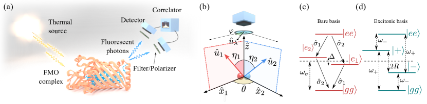
Figure 1: (a) Sketch of the idea of photon-counting spectroscopy. Information about the state of a system $S$ (which might well be a stationary density matrix) is inferred through the statistics of photon-counting events. (b) Geometry of the dimer-detector system. (c) Bare basis of our toy model (6). (d) Excitonic basis which diagonalises the dipole Hamiltonian (6).

Nonlinear laser spectroscopy vs. photon correlation measurements— On a microscopic level, nonlinear spectroscopy measures the nonlinear response functions of a sample, which can be connected to dipole correlation functions Mukamel (1999). For instance, standard techniques such as pump-probe measurements or photon echoes measure the third-order nonlinear susceptibility. Ultrashort pulses prepare a nonequilibrium state, whose evolution is monitored by a probe pulse after fixed time delay. This amounts to a measurement of response functions of the form $\sim\left\langle{d}_{i}(t_{3})\left[{d}_{j}(t_{2}),\left[{d}_{k}(t_{1}),\left[{d}_{l}(0),\varrho_{0}\right]\right]\right]\right\rangle$, where $d_{i}$ denote components of the sample’s dipole operator. Phase matching and control of the laser polarizations allows for additional selectivity, in order to only measure quantum pathways with the desired information Ginsberg et al. (2009); Schlau-Cohen et al. (2011), distinguish homogeneous from inhomogeneous broadening, or detect bath correlations from two-dimensional resonance lineshapes Cho (2008). Multi-color extensions of such measurements further enable the detection of correlations between electronic and vibrational dynamics Lewis et al. (2016).

As we will see below, the conceptually simpler measurement of photon coincidences [see Fig. 3(a)], a central quantity in quantum optics described by Glauber’s second-order correlation function $g^{(2)}(t_{1},t_{2})$, contains similar information, as the fluorescence light can be directly translated into a function of the sample dipole operator. Measurements of bunching and anti-bunching statistics are widely employed to characterize quantum effects in continuously-driven cavity quantum electrodynamics systems Müller et al. (2015); Hamsen et al. (2017), and is recently gaining relevance in other fields, e.g. as a method to achieve super-resolution in biological imaging Tenne et al. (2019). Its most general version meaures coincidences between photons detected at different energy-windows del Valle et al. (2012); Gonzalez-Tudela et al. (2013); Sánchez Muñoz et al. (2014); Ulhaq et al. (2012); Peiris et al. (2015); Silva et al. (2016); Holdaway et al. (2018), described by the frequency-filtered Glauber’s second-order correlation function del Valle et al. (2012):

$$g^{(2)}(\omega_{1},t_{1};\omega_{2},t_{2})=\frac{\langle:\mathcal{T}\big{[}\prod_{i=1}^{2}\hat{E}^{(-)}_{\omega_{i},\Gamma}(t_{i})\hat{E}^{(+)}_{\omega_{i},\Gamma}(t_{i})\big{]}:\rangle}{\prod_{i=1}^{2}\langle\hat{E}^{(-)}_{\omega_{i},\Gamma}(t_{i})\hat{E}^{(+)}_{\omega_{i},\Gamma}(t_{i})\rangle}\,,$$ (1)

where $\mathcal{T}$ ($:$) refers to time (normal) ordering, and with $\hat{E}^{(\pm)}_{\omega_{i},\Gamma}(t)$ the negative/positive frequency parts of the time-dependent electric field operator filtered at the frequency $\omega$ by a Lorentzian filter of linewidth $\Gamma$, $\hat{E}_{\omega,\Gamma}(t)=\frac{\Gamma}{2}\int_{0}^{\infty}\exp[-(i\omega+\Gamma/2)t^{\prime}]\hat{E}(t-t^{\prime})\,\mathrm{d}t^{\prime}$. Here, we will concerned with the simplest case of zero-delay statistics in the stationary regime, where the time-dependence in Eq. (1) can be dropped, $g^{(2)}(\omega_{1},\omega_{2})\equiv\lim_{t\rightarrow\infty}g^{(2)}(\omega_{1},t;\omega_{2},t)$. Even in the zero-delay case, the frequency-filtered electric field involves an integral in time, therefore containing information not only about the stationary values of the density matrix $\rho$, but also about the dynamics of the system, formally encoded in the Liouvillian superoperator $\mathcal{L}$ that generates the evolution of the density matrix, $\dot{\rho}=\mathcal{L}\rho$ Sánchez Muñoz et al. (2019). From Eq. (1) and the definition of $\hat{E}_{\omega,\Gamma}(t)$, it is clear that photon correlation measurements too can be traced back to four-point correlation functions of the sample dipole operators, which is directly proportional to the radiated electric field (see below). Therefore, as pointed out in Ref. Dorfman and Mukamel (2018); Zhang et al. (2018), they can provide similar spectroscopic information as the measurement of the third-order nonlinear response using ultrafast laser, with the important advantage that, rather than using ultrashort pulses to initiate the dynamics, they can be performed in a steady state configuration.

Emission statistics from a single dimer— Now, we demonstrate the use of photon counting statistics to identify coherence in the simplest conceivable composite quantum system: a dimer composed of two dipoles described in the two-level system (TLS) approximation [see Fig. 1(b)]. It forms the simplest toy model to describe the formation of excitonic states in molecular aggregates and their signatures in ultrafast spectroscopy. As a consequence, dimer systems have been widely studied in both theory Kjellberg et al. (2006); Pisliakov et al. (2006); Chen et al. (2010); Yuen-Zhou and Aspuru-Guzik (2011); Bhattacharyya and Fleming (2019) and experiments Halpin et al. (2014), in order to better understand dynamic or spectroscopic features in more complex realistic models of light-harvesting complexes.

Each dipole has a dipolar moment operator $\hat{\mathbf{d}}_{i}=\mathbf{\mu}_{i}(\hat{\sigma}_{i}+\hat{\sigma}^{\dagger}_{i})\mathbf{u}_{i}$, where $\hat{\sigma}_{i}$ is the lowering operator of the $i$-th TLS. Considering the bare energies of the TLSs to be $\omega_{\sigma}$, and that any internal coupling rate is $g\ll\omega_{\sigma}$, the positive-frequency part of far-zone electric field operator radiated by the dimer is given by Scully and Zubairy (2002) $\hat{\mathbf{E}}^{(+)}(\mathbf{r},t)=\mathbf{E_{1}}\hat{\sigma}_{1}(t-|\bm{r}|/c)+\mathbf{E_{2}}\hat{\sigma}_{2}(t-|\bm{r}|/c)$, with $\mathbf{E}_{i}\equiv E_{r}\mu_{i}\sin\eta_{i}\mathbf{x_{i}}$ and $E_{r}\equiv\omega_{\sigma}^{2}/4\pi\epsilon_{0}c^{2}|\mathbf{r}|$. This turns Eq. (1) into a four-point dipole correlation function. The angles $\eta_{i}$ and the unit vector $\mathbf{x_{i}}$ are defined in Fig. 1(b). In the following, we consider that the detectors measure a specific polarization $\mathbf{u}_{\lambda}$, yielding scalar fields $\hat{E}^{(+)}(\mathbf{r},t)=E_{1,\lambda}\hat{\sigma}_{1}(t-|\bm{r}|/c)+E_{2,\lambda}\hat{\sigma}_{2}(t-|\bm{r}|/c)$, where $E_{1(2),\lambda}\equiv\mathbf{E}_{1(2)}\cdot\mathbf{u}_{\lambda}$. Using the angle definitions shown in Fig. 1(b), and omitting from now on the subscript $\lambda$ for convenience, we can write this as

$$E_{1} = E_{r}\mu_{1}\cos\varphi\sin\eta_{1}$$ (2)

$$E_{2} = E_{r}\mu_{2}\cos(\theta-\varphi)\sin\eta_{2}$$ (3)

Thus, $E_{1}$ and $E_{2}$ are determined by the relative orientation of the dipoles $\theta$, the polarizer angle $\varphi$, and the position of the detector. To simplify the discussion, we first consider photon counting statistics on a single detector, as sketched in Fig. 1(b). Thus, Glauber’s zero-delay, second-order correlation function simply reads $g^{(2)}(0)=\langle\hat{E}^{(-)}\hat{E}^{(-)}\hat{E}^{(+)}\hat{E}^{(+)}\rangle/\langle\hat{E}^{(-)}\hat{E}^{(+)}\rangle^{2}$. Writing the correlators in terms of the elements of the density matrix as $\langle\sigma_{1}^{\dagger}\sigma_{2}^{\dagger}\sigma_{1}\sigma_{2}\rangle=\rho_{dd}$, $\langle\sigma_{1}^{\dagger}\sigma_{1}\rangle=\rho_{e_{1}e_{1}}+\rho_{dd}$, $\langle\sigma_{2}^{\dagger}\sigma_{2}\rangle=\rho_{e_{2}e_{2}}+\rho_{dd}$ and $\langle\sigma_{1}^{\dagger}\sigma_{2}\rangle=\rho_{e_{2}e_{1}}$, we straightforwardly obtain

$$g^{(2)}(0)=4(E_{1}E_{2})^{2}\rho_{dd}/\left[E_{1}^{2}\rho_{e_{1}e_{1}}+E_{2}^{2}\rho_{e_{2}e_{2}}\right.\\ \left.+(E_{1}^{2}+E_{2}^{2})\rho_{dd}+2E_{1}E_{2}\Re{\rho_{e_{2}e_{1}}}\right]^{2}.$$ (4)

Bounded photon fluctuations in uncoupled systems— Importantly, Eq. (4) features the steady-state coherence $\rho_{e_{2}e_{1}}$ in the denominator. This terms enters the equation through $\langle\hat{E}^{(-)}\hat{E}^{(+)}\rangle$, which may suggest that a simple measurement of the intensity could suffice to determine the existence or absence of coherence. However, the intensity alone cannot distinguish coherence without an a-priori knowledge of the dipole strength of the sample.

On the other hand, a measurement of $g^{(2)}(0)$ can unambiguously verify the presence of excitonic coherence in the steady state. To prove this, we will now evaluate Eq. (4) for a reference case in which no coherence exists. This reference case consists of two TLSs with no coherence, neither in the bare or the excitonic (energy) basis and no population imbalance, i.e. a state that fulfils the following three conditions: (I) $\rho_{e_{1}e_{2}}=\rho_{e_{2}e_{1}}=0$, (II) $\rho_{e_{1}e_{1}}=\rho_{e_{2}e_{2}}\equiv p$, and (III) $\rho_{dd}=p^{2}(1+p)^{2}$. The last equation comes from the assumption $\langle\sigma_{1}^{\dagger}\sigma_{2}^{\dagger}\sigma_{1}\sigma_{2}\rangle=\langle\sigma_{1}^{\dagger}\sigma_{1}\rangle\langle\sigma_{2}^{\dagger}\sigma_{2}\rangle$. This is the expected situation when the dimer is excited by a light source with a bandwidth that is much larger than the detuning $\Delta$ between the two TLSs. For instance, for our discussion to remain valid for the excitation by sunlight, we require the detuning to be small enough for the variation of the light intensity with the wavelength to be negligible. We can then show that photon correlations allow to identify states where these conditions are not fulfilled. Applying these conditions in Eq. (4), we find $g^{(2)}(0)=4(E_{1}E_{2})^{2}/\left(E_{1}^{2}+E_{2}^{2}\right)^{2}$, which we write in terms of the ratio $r=E_{2}/E_{1}$ as $\mathinner{g^{(2)}(0)}=4r^{2}/(1+r^{2})^{2}$. Its maximum value of $1$ is obtained at $r=1$. This is the expected result for two uncoupled TLS, in which the two emitters are independent of each other, which is an intuitive outcome in the absence of coherence. Hence, we find the criterion

$$\mathinner{g^{(2)}(0)}>1$$ (5)

to identify coherence, i.e. the limit of two uncoupled emitters can only be surpassed in the presence of steady state coherence in the dimer.

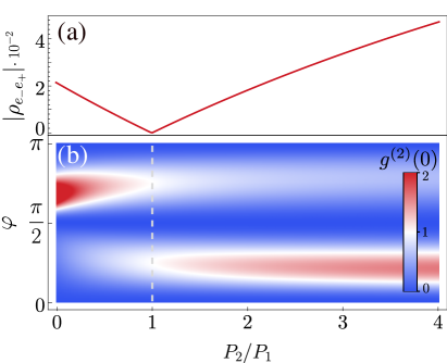
Figure 2: (a) Coherence between excitonic states versus the pumping anisotropy $P_{2}/P_{1}$. When $P_{1}=P_{2}$, no excitonic coherence exists. (b) Dependence of $g^{(2)}(0)$ on the polarization angle $\varphi$ and the anisotropy $P_{2}$. Parameters: $R=4\gamma$, $\beta=\pi/3$, $J=2\gamma$, $\theta=\pi/2$, $P_{1}=0.1\gamma$. Coherence is evidenced by the existence of regions with $g_{2}^{(0)}>1$.

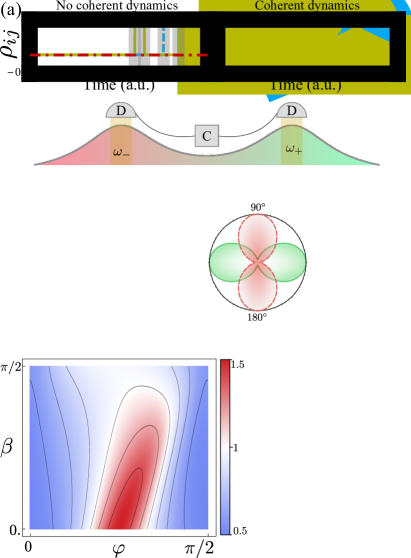
Figure 3: (a) Monte Carlo trajectories depicting $\rho_{e_{1}e_{1}}$ (solid, yellow), $\rho_{e_{2}e_{2}}$ (dashed, blue), and $\rho_{e_{1}e_{2}}$ (dot-dashed, red) during the process of absorbing and emitting several photons, with and without coherent couplings. For $P_{1}=P_{2}$, the oscillatory dynamics of the coherences average to zero steady-state coherence. (b) Sketch of a frequency-resolved correlation setup measuring correlations between the two spectral peaks at $\omega_{\pm}$. (c) Polarization measurements of the spectrum of emission at frequencies $\omega_{\pm}$ for different values of coherent coupling $J=R\cos\beta$ and inter-dipole angle $\theta$. (d-e) Cross-correlation measurements at $\theta=\pi/2$ versus detection polarization for different values of $\beta$. Parameters: $R=2\gamma$, $P_{1}=P_{2}=0.1\gamma$, $\Gamma=\gamma$.

Specific model— We now provide a particular example on how coherence can be detected by fulfilling this inequality. To this end, we introduce a driven-dissipative dynamical model of the dimers in which we will tune the steady state coherence by introducing ad hoc asymmetric incoherent pumping.

The model consists of two coupled TLSs with frequencies $\omega_{\sigma}\pm\Delta/2$, described by the dipole Hamiltonian

$$\hat{H}_{d}=(\omega_{\sigma}-\Delta/2)\hat{\sigma}_{1}^{\dagger}\hat{\sigma}_{1}+(\omega_{\sigma}+\Delta/2)\hat{\sigma}_{2}^{\dagger}\hat{\sigma}_{2}+J(\hat{\sigma}_{1}^{\dagger}\hat{\sigma}_{2}+\text{H.c.}),$$ (6)

where $J$ denotes coherent coupling between the TLSs. The eigenstates for ${J=0}$ correspond to the bare or site basis, $\{|gg\rangle,|e_{1}\rangle,|e_{2}\rangle,|ee\rangle\}$, see Fig. 1(c). In the general case ${J\neq 0}$, the eigenstates in the one-excitation subspace are $|+\rangle=c|e_{1}\rangle+s|e_{2}\rangle$ and $|-\rangle=s|e_{1}\rangle-c|e_{2}\rangle$, where $c=1/\sqrt{1+\xi^{-2}}$, $s=1/\sqrt{1+\xi^{2}}$, $\xi=J/(\Delta/2+R)$ and $R=\sqrt{J^{2}+(\Delta/2)^{2}}$, so that the corresponding energies are $\omega_{\pm}=\omega_{\sigma}\pm R$. We will consider the general case in which $R\neq 0$ and greater than the natural linewidths in the system, i.e. we will assume that one can observe two spectrally resolved peaks in the emission at the energies $\omega_{\pm}$. In order to keep the peak separation fixed, regardless of its possible origin, we parametrize $\Delta$ and $J$ by a mixing angle $\beta$ as $J=R\cos\beta$ and $\Delta/2=R\sin\beta$. Thus, the case $\beta=0$ corresponds to two peaks originating from two coupled, resonant dipoles, and $\beta=\pi/2$ to two uncoupled, detuned dipoles.

The driven-dissipative dynamics of the dimers in the presence of losses and incoherent driving is described by the master equation $\dot{\rho}=-i[H,\rho]+\sum_{i}\gamma\mathcal{D}_{\sigma_{i}}\{\rho\}/2+\sum_{i}P_{i}\mathcal{D}_{\sigma_{i}^{\dagger}}\{\rho\}/2,$ with $\mathcal{D}_{\mathcal{O}}\{\rho\}\equiv 2\mathcal{O}\rho\mathcal{O}^{\dagger}-\mathcal{O}^{\dagger}\mathcal{O}\rho-\rho\mathcal{O}^{\dagger}\mathcal{O}$, where $\gamma$ is the decay rate of both dimers and $P_{i}$ the incoherent pumping rate of the $i$-th dimer. Importantly, we allow for different incoherent excitation rates that can give rise to population imbalance. This is relevant since coherences in the excitonic basis are given by $\rho_{e_{-}e_{+}}=cs(\rho_{e_{1}e_{1}}-\rho_{e_{2}e_{2}})+s^{2}\rho_{e_{2}e_{1}}-c^{2}\rho_{e_{1}e_{2}}$. Thus, in order to have coherence in the excitonic basis we need coherence and/or population imbalance in the site basis, which we can enforce by setting $J\neq 0$ (so $c\neq 0$) and $P_{1}\neq P_{2}$. As shown in Fig. 2(a), the pumping imbalance gives rise to steady state coherence between the excitonic states of the dimer which is directly proportional to the asymmetry of the pumps. This allows us to illustrate the potential of $g^{(2)}(0)$ measurements to unveil coherences in the excitonic basis, as we demonstrate in Fig. 2(b), where $g^{(2)}(0)$ is plotted vs the anisotropy of the pumping and the polarizer angle of the detector setup. This plot reveals regions with $g^{(2)}(0)>1$ fulfilling the criterion Eq. (5) and hence signalling the presence of steady state coherence in the system. Only when there is coherence in the steady state, the variation of the polarizer angle yields a value larger than unity for some angle that depends on the dimer parameters, and thus enables the direct detection of steady state coherence. This is the first main result of our paper.

Frequency-resolved measurements— The previous analysis has been devoted to revealing coherence in the stationary density matrix of the system using photon correlation measurements. Now, we explore how frequency-resolved measurements [see Eq. (1)] introduce a time resolution that allows to reveal transient coherent dynamics even when these average to zero in the steady state [see Fig. 3(a)], allowing to distinguish this case from that of detuned, uncoupled emitters. In our model, we can describe coherent dynamics that yield zero stationary coherences by setting $J\neq 0$, $P_{1}=P_{2}$, which is the case we consider from now on.

From now on, we will be concerned with the light emitted at the two possible transition energies between eigenstates, $\omega_{\pm}$, see Fig. 3(b). Figure 3(c) shows the polarization profile of the light emitted at these two frequencies, given by $S(\omega_{\pm})=\lim_{t\rightarrow\infty}\langle\hat{E}^{(-)}_{\omega_{\pm},\Gamma}(t)\hat{E}^{(+)}_{\omega_{\pm},\Gamma}(t)\rangle$, for several combinations of $\beta$ and $\theta$. If we consider that most of the emission will come from the single-excitation subspace, so that $S(\omega_{\pm})\propto|\langle gg|\hat{E}^{(+)}|\pm\rangle|^{2}$, we expect

$$S(\omega_{\pm})\propto E_{1/2}^{2}c^{2}+E_{2/1}^{2}s^{2}\pm 2csE_{1}E_{2}.$$ (7)

These equations can qualitatively explain the features in Fig. 3(c). Namely, for $\theta=0$, the two dipoles are aligned, so both peaks exhibit the same dependence with the polarizer angle $\varphi$. For $\theta=\pi/2$, the two are orthogonal, $E_{1}\propto\cos\varphi$, $E_{2}\propto\sin\varphi$. A frequency-resolved polarization measurement therefore provides valuable information about the internal structure of the dimer, since the angle between the two lobes gives an estimate of $\theta$. However, the information obtained about the presence of coherent dynamics is limited: only in the case of aligned dipoles and $\beta=\pi/2$ the presence of two peaks with same $\varphi$-dependence unambiguously signifies the absence of coherent coupling. All the other cases shown in Fig. 3(c), are ambiguous, i.e., one cannot tell whether the peaks are created by uncoupled or coupled emitters.

Coherent couplings can, however, be unveiled by correlation measurements in the frequency domain. Without loss of generality, we focus on the case $\theta=\pi/2$. We analyse cross-correlations between the two emission peaks [see Fig. 3(b)], since any possible two-photon de-excitation process from $|ee\rangle$ will involve photons of the two frequencies $\omega_{\pm}$ [see Fig. 1(c)]. As we show in Figs. 3(d-e), measuring this cross-peak correlation for different values of $\varphi$ reveals bunching features [$g^{(2)}(\omega_{+},\omega_{-})>1$] around $\varphi=\pi/4$ only in the presence of coherent coupling, even if the steady-state coherence is zero in all cases. To qualitatively understand this observation, we note that, at $\varphi=\pi/4$, coherent coupling yields a destructive interference of the emission at $\omega_{-}$ originating from the first-excitation subspace, i.e. $S(\omega_{-})=0$ in Eq. (7). Consequently, any emission detected at $\omega_{-}$ must originate from a two-photon cascade from the doubly-excited state $|ee\rangle$ to state $|+\rangle$, and will therefore show strong correlations with subsequently emitted photons from $|+\rangle$ to $|gg\rangle$ at frequency $\omega_{+}$. In the absence of coupling, the two peaks must originate from two independent, detuned emitters, and one recovers the expected result for uncorrelated emission, $g^{(2)}(\omega_{+},\omega_{-})\approx 1$ . Note the qualitative difference between coupled and uncoupled cases in Fig. 3(e) as compared to the plots in panel (c).
Conclusions— We have established the potential of steady-state photon correlation measurements as a novel tool for molecular spectroscopy. The analysis of the emission statistics of a dimer model revealed that it is possible to detect the presence of environment-induced steady state coherence in the system. In frequency-resolved measurements, we observe that, akin to cross-peaks in two-dimensional laser spectroscopy Cho (2008), the bunching of photons at two different frequencies indicates coherent coupling between the dipoles. The strength of the coherent coupling can be read off the bunching ratio, and provides direct access to the bare emitter frequencies, whose accurate determination is of critical importance to relate structural and optical properties in molecular aggregates Adolphs et al. (2007); Cheng and Fleming (2009); Milder et al. (2010). Our results clearly demonstrate that photon correlations can provide a new valuable tool for experimentalists and open new avenues in the field of quantum spectroscopy Dorfman et al. (2016); Schlawin et al. (2018).

Supplementary Material

Analytical expressions for steady state density matrix elements

The master equation analysed in the main text

$$\dot{\rho}=-i[H,\rho]+\sum_{i}\gamma\mathcal{D}_{\sigma_{i}}\{\rho\}/2+\sum_{i}P_{i}\mathcal{D}_{\sigma_{i}^{\dagger}}\{\rho\}/2$$ (S1)

yields the following stationary expectation values:

$$\langle\sigma_{1}^{\dagger}\sigma_{1}\rangle=\frac{4J^{2}(\tilde{P}_{1}+\tilde{P}_{2})(P_{1}+P_{2})+P_{1}\tilde{P}_{2}\chi}{4J^{2}(\tilde{P}_{1}+\tilde{P}_{2})^{2}+\tilde{P}_{1}\tilde{P}_{2}\chi},$$ (S2a)

$$\langle\sigma_{2}^{\dagger}\sigma_{2}\rangle=\frac{4J^{2}(\tilde{P}_{1}+\tilde{P}_{2})(P_{1}+P_{2})+\tilde{P}_{1}P_{2}\chi}{4J^{2}(\tilde{P}_{1}+\tilde{P}_{2})^{2}+\tilde{P}_{1}\tilde{P}_{2}\chi},$$ (S2b)

$$\langle\sigma_{1}^{\dagger}\sigma_{2}\rangle=\frac{-2iJ\gamma(\tilde{P}_{1}-\tilde{P}_{2})[\tilde{P}_{1}+\tilde{P}_{2}+2i\Delta]}{4J^{2}(\tilde{P}_{1}+\tilde{P}_{2})^{2}+\tilde{P}_{1}\tilde{P}_{2}\chi},$$ (S2c)

$$\langle\sigma_{1}^{\dagger}\sigma_{2}^{\dagger}\sigma_{1}\sigma_{2}\rangle=\frac{4J^{2}(P_{1}+P_{2})^{2}+P_{1}P_{2}\chi}{4J^{2}(\tilde{P}_{1}+\tilde{P}_{2})^{2}+\tilde{P}_{1}\tilde{P}_{2}\chi},$$ (S2d)

where $\tilde{P}_{i}\equiv P_{i}+\gamma$ and $\chi\equiv(\tilde{P}_{1}+\tilde{P}_{2})^{2}+4\Delta^{2}$. It is important to notice that coherences $\rho_{e_{1}e_{2}}$, given by the correlator $\langle\sigma_{1}^{\dagger}\sigma_{2}\rangle$, are only different from zero provided $J\neq 0$ and $P_{1}\neq P_{2}$. The later condition is also a requirement to obtain steady-state population imbalance on the bare basis, which is given by:

$$\rho_{e_{1}e_{1}}-\rho_{e_{2}e_{2}}=\frac{(P_{1}-P_{2})\gamma\chi}{4J^{2}(\tilde{P}_{1}+\tilde{P}_{2})^{2}+\tilde{P}_{1}\tilde{P}_{2}\chi}.$$ (S3)

As we discuss in the main text, excitonic coherence is given by

$$\rho_{e_{-}e_{+}}=cs(\rho_{e_{1}e_{1}}-\rho_{e_{2}e_{2}})+s^{2}\rho_{e_{2}e_{1}}-c^{2}\rho_{e_{1}e_{2}},$$ (S4)

which means that driving imbalance $P_{1}\neq P_{2}$ is also a requisite for excitonic coherence, which can therefore by tuned by introducing ad hoc asymmetric incoherent driving.

Detection of coherence using $g^{(2)}(0)$: Dependence on system parameters

In Fig. S1, we extend the simulations in Fig. 2 in the main text to different combinations of the angle between bare dipoles $\theta$ and mixing angle $\beta$. We find that $\theta$ does not impede our ability to detect steady state coherence, i.e. if bunching $g^{(2)}(0)>1$ signalling coherence is measured for a given dipole-dipole angle $\theta$, it would also be measured for any other angle. Coherence is evidenced by the criterion $g^{(2)}(0)>1$ except in the limit case $\beta=0$.

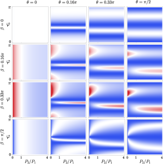
Figure S1: Dependence of $g^{2}(0)$ on the polarization angle and the anisotropy $P_{2}/P_{1}$, as in Fig. 2(b). The two free parameters of the dimer system, the mixing angle $\beta$ and the angle between the dipoles $\theta$ are varied.

Frequency-resolved photon correlation measurements

In the main text, we have provided an intuitive explanation for our findings on the frequency-resolved correlations between peaks. Beyond this explanation, we can also qualitatively describe our findings by computing transition matrix elements as we did for the spectrum peaks $S(\omega_{\pm})$. To do this, we consider, at zero time delay, that the quantity $G^{(2)}(\omega_{+},\omega_{-})=\langle E^{(-)}_{\omega_{+},\Gamma}E^{(-)}_{\omega_{-},\Gamma}E^{(+)}_{\omega_{+},\Gamma}E^{(+)}_{\omega_{-},\Gamma}\rangle$ in the numerator of Eq. (1) is given by

$$G^{(2)}(\omega_{+},\omega_{-})\propto|\sum_{j=+,-}\langle gg|\hat{E}^{(+)}|j\rangle\langle j|\hat{E}^{(+)}|ee\rangle|^{2}\propto|E_{1}E_{2}|^{2}\propto\cos^{2}\varphi\cos^{2}(\theta-\varphi).$$ (S5)

To see how this qualitatively explains the dependence of $g^{(2)}(\omega_{+},\omega_{-})$ on the polarisation angle, $\varphi$, and the mixing angle, $\beta$, let us consider the two following limiting cases:

$\beta=0$ (strongly-coupled)

For $\beta=0$, we have $J=R$, and $c=s=1/\sqrt{2}$, so $S(\omega_{+})S(\omega_{-})\propto\left[\cos^{2}\varphi-\cos^{2}(\theta-\varphi)\right]^{2}$, giving

$$g^{(2)}(\omega_{1},\omega_{2})\propto\frac{\cos^{2}\varphi\cos^{2}(\theta-\varphi)}{\left[\cos^{2}\varphi-\cos^{2}(\theta-\varphi)\right]^{2}}.$$ (S6)

For $\theta=\pi/2$, this is equal to

$$g^{(2)}(\omega_{1},\omega_{2})\propto\frac{\cos^{2}\varphi\sin^{2}\varphi}{\left(\cos^{2}\varphi-\sin^{2}\varphi\right)^{2}}.$$ (S7)

$\beta=\pi/2$ (uncoupled)

For $\beta=\pi/2$, $J=0$, $c=0$, $s=1$, giving $S(\omega_{+})S(\omega_{-})=E_{1}^{2}E_{2}^{2}$, and $g^{(2)}(\omega_{1},\omega_{2})\propto 1$.

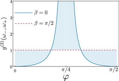
Figure S2: Analytical estimation of the frequency-resolved correlation function between the two emission peaks, $g^{(2)}(\omega_{-},\omega_{+})$ for the two limiting cases of strongly-coupled ($\beta=0$) and uncoupled ($\beta=\pi/2$) emitters.

These two possible expressions are plotted in Fig. S2, and qualitatively replicate the characteristic feature observed in our exact, numerical calculations shown in in Fig. 3(d), namely the emergence of bunching in the presence of coherent dynamics. The expressions obtained here only qualitatively match the exact result due to the contributions to the spectrum $S(\omega_{\pm})$ from the doubly excited state $|ee\rangle$, not considered in these analytical estimations, and to the finite filter linewidth $\Gamma$.

References

- Vinjanampathy and Anders (2016) S. Vinjanampathy and J. Anders, Quantum thermodynamics, Contemporary Physics 57, 545 (2016).
- Binder et al. (2018) F. Binder, L. A. Correa, C. Cogolin, J. Anders, and G. Adesso, eds., Thermodynamics in the Quantum Regime: Fundamental Aspects and New Directions, (Springer International Publishing, 2018).
- Streltsov et al. (2017) A. Streltsov, G. Adesso, and M. B. Plenio, Colloquium: Quantum coherence as a resource, Rev. Mod. Phys. 89, 041003 (2017).
- Lostaglio et al. (2015) M. Lostaglio, K. Korzekwa, D. Jennings, and T. Rudolph, Quantum Coherence, Time-Translation Symmetry, and Thermodynamics, Phys. Rev. X 5, 021001 (2015).
- Li et al. (2012) C.-M. Li, N. Lambert, Y.-N. Chen, G.-Y. Chen, and F. Nori, Witnessing quantum coherence: from solid-state to biological systems, Scientific Report 2, 885 (2012).
- Marcus et al. (2019) M. Marcus, G. C. Knee, and A. Datta, Towards a Spectroscopic Protocol for Unambiguous Detection of Quantum Coherence in Excitonic Energy Transport, Faraday Discussions 221, 110 (2019).
- Scully et al. (2011) M. O. Scully, K. R. Chapin, K. E. Dorfman, M. B. Kim, and A. Svidzinsky, Quantum heat engine power can be increased by noise-induced coherence, Proceedings of the National Academy of Sciences 108, 15097 (2011).
- Mitchison et al. (2015) M. T. Mitchison, M. P. Woods, J. Prior, and M. Huber, Coherence-assisted single-shot cooling by quantum absorption refrigerators, New Journal of Physics 17, 115013 (2015).
- Wertnik et al. (2018) M. Wertnik, A. Chin, F. Nori, and N. Lambert, Optimizing co-operative multi-environment dynamics in a dark-state-enhanced photosynthetic heat engine, J. Chem. Phys. 149, 084112 (2018).
- Wang et al. (2019) L. Wang, M. A. Allodi, and G. S. Engel, Quantum coherences reveal excited-state dynamics in biophysical systems, Nat. Rev. Chem. 3, 477 (2019).
- Allahverdyan et al. (2004) A. E. Allahverdyan, R. Balian, and T. M. Nieuwenhuizen, Maximal work extraction from finite quantum systems, Europhysics Letters (EPL) 67, 565 (2004).
- Klatzow et al. (2019) J. Klatzow, J. N. Becker, P. M. Ledingham, C. Weinzetl, K. T. Kaczmarek, D. J. Saunders, J. Nunn, I. A. Walmsley, R. Uzdin, and E. Poem, Experimental Demonstration of Quantum Effects in the Operation of Microscopic Heat Engines, Phys. Rev. Lett. 122, 110601 (2019).
- Dorfman et al. (2018) K. E. Dorfman, D. Xu, and J. Cao, Efficiency at maximum power of a laser quantum heat engine enhanced by noise-induced coherence, Phys. Rev. E 97, 042120 (2018).
- Scholes et al. (2011) G. D. Scholes, G. R. Fleming, A. Olaya-Castro, and R. van Grondelle, Lessons from nature about solar light harvesting, Nature Chemistry 3, 763 (2011).
- Romero et al. (2017) E. Romero, V. I. Novoderezhkin, and R. van Grondelle, Quantum design of photosynthesis for bio-inspired solar-energy conversion, Nature 543, 355 (2017).
- Scholes et al. (2017) G. D. Scholes, G. R. Fleming, L. X. Chen, A. Aspuru-Guzik, A. Buchleitner, D. F. Coker, G. S. Engel, R. van Grondelle, A. Ishizaki, D. M. Jonas, J. S. Lundeen, J. K. McCusker, S. Mukamel, J. P. Ogilvie, A. Olaya-Castro, M. A. Ratner, F. C. Spano, K. B. Whaley, and X. Zhu, Using coherence to enhance function in chemical and biophysical systems, Nature 543, 647 (2017).
- Mukamel (1999) S. Mukamel, Principles of Nonlinear Optical Spectroscopy, Oxford series in optical and imaging sciences (Oxford University Press, Oxford, UK, 1999).
- Brumer and Shapiro (2012) P. Brumer and M. Shapiro, Molecular response in one-photon absorption via natural thermal light vs. pulsed laser excitation, Proceedings of the National Academy of Sciences 109, 19575 (2012).
- Duan et al. (2017) H.-G. Duan, V. I. Prokhorenko, R. J. Cogdell, K. Ashraf, A. L. Stevens, M. Thorwart, and R. J. D. Miller, Nature does not rely on long-lived electronic quantum coherence for photosynthetic energy transfer, Proceedings of the National Academy of Sciences 114, 8493 (2017).
- Chenu and Brumer (2016) A. Chenu and P. Brumer, Transform-limited-pulse representation of excitation with natural incoherent light, The Journal of Chemical Physics 144, 044103 (2016).
- Chan et al. (2018) H. C. H. Chan, O. E. Gamel, G. R. Fleming, and K. B. Whaley, Single-photon absorption by single photosynthetic light-harvesting complexes, Journal of Physics B: Atomic, Molecular and Optical Physics 51, 054002 (2018).
- Dodin and Brumer (2019) A. Dodin and P. Brumer, Light-induced processes in nature: Coherences in the establishment of the nonequilibrium steady state in model retinal isomerization, The Journal of Chemical Physics 150, 184304 (2019).
- Fujihashi et al. (2019) Y. Fujihashi, R. Shimizu, and A. Ishizaki, Generation of pseudo-sunlight via quantum entangled photons and the interaction with molecules, arXiv e-prints , arXiv:1904.11669 (2019).
- Iles-Smith et al. (2014) J. Iles-Smith, N. Lambert, and A. Nazir, Environmental dynamics, correlations, and the emergence of noncanonical equilibrium states in open quantum systems, Phys. Rev. A 90, 032114 (2014).
- Tscherbul and Brumer (2015) T. V. Tscherbul and P. Brumer, Quantum coherence effects in natural light-induced processes: cisâtrans photoisomerization of model retinal under incoherent excitation, Phys. Chem. Chem. Phys. 17, 30904 (2015).
- Iles-Smith et al. (2016) J. Iles-Smith, A. G. Dijkstra, N. Lambert, and A. Nazir, Energy transfer in structured and unstructured environments: Master equations beyond the Born-Markov approximations, J. Chem. Phys. 144, 044110 (2016).
- Dodin et al. (2016) A. Dodin, T. V. Tscherbul, and P. Brumer, Coherent dynamics of V-type systems driven by time-dependent incoherent radiation, The Journal of Chemical Physics 145, 244313 (2016).
- Shatokhin et al. (2018) V. N. Shatokhin, M. Walschaers, F. Schlawin, and A. Buchleitner, Coherence turned on by incoherent light, New Journal of Physics 20, 113040 (2018).
- Tscherbul and Brumer (2018) T. V. Tscherbul and P. Brumer, Non-equilibrium stationary coherences in photosynthetic energy transfer under weak-field incoherent illumination, The Journal of Chemical Physics 148, 124114 (2018).
- Brumer (2018) P. Brumer, Shedding (Incoherent) Light on Quantum Effects in Light-Induced Biological Processes, The Journal of Physical Chemistry Letters 9, 2946 (2018), pMID: 29763314.
- Romero et al. (2014) E. Romero, R. Augulis, V. I. Novoderezhkin, M. Ferretti, J. Thieme, D. Zigmantas, and R. van Grondelle, Quantum coherence in photosynthesis for efficient solar-energy conversion, Nature Physics 10, 676 (2014).
- Fuller et al. (2014) F. D. Fuller, J. Pan, A. Gelzinis, V. Butkus, S. S. Senlik, D. E. Wilcox, C. F. Yocum, L. Valkunas, D. Abramavicius, and J. P. Ogilvie, Vibronic coherence in oxygenic photosynthesis, Nature Chemistry 6, 706 (2014).
- Hettich et al. (2002) C. Hettich, C. Schmitt, J. Zitzmann, S. Kühn, I. Gerhardt, and V. Sandoghdar, Nanometer Resolution and Coherent Optical Dipole Coupling of Two Individual Molecules, Science 298, 385 (2002).
- Krüger et al. (2010) T. P. Krüger, V. I. Novoderezhkin, C. Ilioaia, and R. van Grondelle, Fluorescence Spectral Dynamics of Single LHCII Trimers, Biophysical Journal 98, 3093 (2010).
- Hildner et al. (2013) R. Hildner, D. Brinks, J. B. Nieder, R. J. Cogdell, and N. F. van Hulst, Quantum Coherent Energy Transfer over Varying Pathways in Single Light-Harvesting Complexes, Science 340, 1448 (2013).
- Wientjes et al. (2014) E. Wientjes, J. Renger, A. G. Curto, R. Cogdell, and N. F. van Hulst, Strong antenna-enhanced fluorescence of a single light-harvesting complex shows photon antibunching, Nature Communications 5, 4236 (2014).
- Liebel et al. (2018) M. Liebel, C. Toninelli, and N. F. van Hulst, Room-temperature ultrafast nonlinear spectroscopy of a single molecule, Nature Photonics 12, 45 (2018).
- Kyeyune et al. (2019) F. Kyeyune, J. L. Botha, B. van Heerden, P. Malỳ, R. van Grondelle, M. Diale, and T. P. J. Krüger, Strong plasmonic fluorescence enhancement of individual plant light-harvesting complexes, Nanoscale 11, 15139 (2019).
- del Valle et al. (2012) E. del Valle, A. Gonzalez-Tudela, F. P. Laussy, C. Tejedor, and M. J. Hartmann, Theory of Frequency-Filtered and Time-Resolved -Photon Correlations, Phys. Rev. Lett. 109, 183601 (2012).
- Gonzalez-Tudela et al. (2013) A. Gonzalez-Tudela, F. P. Laussy, C. Tejedor, M. J. Hartmann, and E. del Valle, Two-photon spectra of quantum emitters, New J. Phys. 15, 033036 (2013).
- Sánchez Muñoz et al. (2014) C. Sánchez Muñoz, E. del Valle, C. Tejedor, and F. P. Laussy, Violation of classical inequalities by photon frequency filtering, Phys. Rev. A 90, 052111 (2014).
- Ulhaq et al. (2012) A. Ulhaq, S. Weiler, S. M. Ulrich, R. Roßbach, M. Jetter, and P. Michler, Cascaded single-photon emission from the Mollow triplet sidebands of a quantum dot, Nat. Photon. 6, 238 (2012).
- Peiris et al. (2015) M. Peiris, B. Petrak, K. Konthasinghe, Y. Yu, Z. C. Niu, and A. Muller, Two-color photon correlations of the light scattered by a quantum dot, Phys. Rev. B 91, 195125 (2015).
- Silva et al. (2016) B. Silva, C. Sánchez Muñoz, D. Ballarini, A. G. Tudela, M. de Giorgi, G. Gigli, K. W. West, L. Pfeiffer, E. del Valle, D. Sanvitto, and F. P. Laussy, The colored Hanbury Brown–Twiss effect, Scientific Report 6, 37980 (2016).
- Holdaway et al. (2018) D. I. H. Holdaway, V. Notararigo, and A. Olaya-Castro, Perturbation approach for computing frequency- and time-resolved photon correlation functions, Phys. Rev. A 98, 063828 (2018).
- Cho (2008) M. Cho, Coherent Two-Dimensional Optical Spectroscopy, Chemical Reviews 108, 1331 (2008), pMID: 18363410.
- Hamm and Zanni (2011) P. Hamm and M. Zanni, Concepts and Methods of 2D Infrared Spectroscopy (Cambridge University Press, 2011).
- Adolphs et al. (2007) J. Adolphs, F. Müh, M. E.-A. Madjet, and T. Renger, Calculation of pigment transition energies in the FMO protein, Photosynthesis Research 95, 197 (2007).
- Cheng and Fleming (2009) Y.-C. Cheng and G. R. Fleming, Dynamics of Light Harvesting in Photosynthesis, Annual Review of Physical Chemistry 60, 241 (2009), pMID: 18999996.
- Milder et al. (2010) M. T. W. Milder, B. Brüggemann, R. van Grondelle, and J. L. Herek, Revisiting the optical properties of the FMO protein, Photosynthesis Research 104, 257 (2010).
- Ginsberg et al. (2009) N. S. Ginsberg, Y.-C. Cheng, and G. R. Fleming, Two-Dimensional Electronic Spectroscopy of Molecular Aggregates, Accounts of Chemical Research 42, 1352 (2009).
- Schlau-Cohen et al. (2011) G. S. Schlau-Cohen, A. Ishizaki, and G. R. Fleming, Two-dimensional electronic spectroscopy and photosynthesis: Fundamentals and applications to photosynthetic light-harvesting, Chemical Physics 386, 1 (2011).
- Lewis et al. (2016) N. H. C. Lewis, N. L. Gruenke, T. A. A. Oliver, M. Ballottari, R. Bassi, and G. R. Fleming, Observation of Electronic Excitation Transfer Through Light Harvesting Complex II Using Two-Dimensional ElectronicâVibrational Spectroscopy, The Journal of Physical Chemistry Letters 7, 4197 (2016).
- Müller et al. (2015) K. Müller, A. Rundquist, K. A. Fischer, T. Sarmiento, K. G. Lagoudakis, Y. A. Kelaita, C. Sánchez Muñoz, E. del Valle, F. P. Laussy, and J. Vučković, Coherent generation of nonclassical light on chip via detuned photon blockade, Phys. Rev. Lett. 114, 233601 (2015).
- Hamsen et al. (2017) C. Hamsen, K. N. Tolazzi, T. Wilk, and G. Rempe, Two-Photon Blockade in an Atom-Driven Cavity QED System, Phys. Rev. Lett. 118, 133604 (2017).
- Tenne et al. (2019) R. Tenne, U. Rossman, B. Rephael, Y. Israel, A. Krupinski-Ptaszek, R. Lapkiewicz, Y. Silberberg, and D. Oron, Super-resolution enhancement by quantum image scanning microscopy, Nat. Photon. 13, 116 (2019).
- Sánchez Muñoz et al. (2019) C. Sánchez Muñoz, B. Buča, J. Tindall, A. González-Tudela, D. Jaksch, and D. Porras, Symmetries and conservation laws in quantum trajectories: Dissipative freezing, Phys. Rev. A 100, 042113 (2019).
- Dorfman and Mukamel (2018) K. E. Dorfman and S. Mukamel, Multidimensional photon correlation spectroscopy of cavity polaritons, Proceedings of the National Academy of Sciences 115, 1451 (2018).
- Zhang et al. (2018) Z. Zhang, P. Saurabh, K. E. Dorfman, A. Debnath, and S. Mukamel, Monitoring polariton dynamics in the LHCII photosynthetic antenna in a microcavity by two-photon coincidence counting, The Journal of Chemical Physics 148, 074302 (2018).
- Kjellberg et al. (2006) P. Kjellberg, B. Brüggemann, and T. o. Pullerits, Two-dimensional electronic spectroscopy of an excitonically coupled dimer, Phys. Rev. B 74, 024303 (2006).
- Pisliakov et al. (2006) A. V. Pisliakov, T. Mančal, and G. R. Fleming, Two-dimensional optical three-pulse photon echo spectroscopy. II. Signatures of coherent electronic motion and exciton population transfer in dimer two-dimensional spectra, The Journal of Chemical Physics 124, 234505 (2006).
- Chen et al. (2010) L. Chen, R. Zheng, Q. Shi, and Y. Yan, Two-dimensional electronic spectra from the hierarchical equations of motion method: Application to model dimers, The Journal of Chemical Physics 132, 024505 (2010).
- Yuen-Zhou and Aspuru-Guzik (2011) J. Yuen-Zhou and A. Aspuru-Guzik, Quantum process tomography of excitonic dimers from two-dimensional electronic spectroscopy. I. General theory and application to homodimers, The Journal of Chemical Physics 134, 134505 (2011).
- Bhattacharyya and Fleming (2019) P. Bhattacharyya and G. R. Fleming, Two-Dimensional Electronic–Vibrational Spectroscopy of Coupled Molecular Complexes: A Near-Analytical Approach, The Journal of Physical Chemistry Letters 10, 2081 (2019).
- Halpin et al. (2014) A. Halpin, P. J. M. Johnson, R. Tempelaar, R. S. Murphy, J. Knoester, T. L. C. Jansen, and R. J. D. Miller, Two-dimensional spectroscopy of a molecular dimer unveils the effects of vibronic coupling on exciton coherences, Nature Chemistry 6, 196 (2014).
- Scully and Zubairy (2002) M. O. Scully and M. S. Zubairy, Quantum optics (Cambridge University Press, 2002).
- Dorfman et al. (2016) K. E. Dorfman, F. Schlawin, and S. Mukamel, Nonlinear optical signals and spectroscopy with quantum light, Rev. Mod. Phys. 88, 045008 (2016).
- Schlawin et al. (2018) F. Schlawin, K. E. Dorfman, and S. Mukamel, Entangled Two-Photon Absorption Spectroscopy, Accounts of Chemical Research 51, 2207 (2018).