FPT Algorithms for Diverse Collections of Hitting Sets

Abstract

In this work, we study the $d$-Hitting Set and Feedback Vertex Set problems through the paradigm of finding diverse collections of $r$ solutions of size at most $k$ each, which has recently been introduced to the field of parameterized complexity [Baste et al., 2019]. This paradigm is aimed at addressing the loss of important side information which typically occurs during the abstraction process which models real-world problems as computational problems. We use two measures for the diversity of such a collection: the sum of all pairwise Hamming distances, and the minimum pairwise Hamming distance. We show that both problems are FPT in $k+r$ for both diversity measures. A key ingredient in our algorithms is a (problem independent) network flow formulation that, given a set of ‘base’ solutions, computes a maximally diverse collection of solutions. We believe that this could be of independent interest.

20(0, 12.5) 20(-0.25, 12.9)

Keywords: Solution Diversity; Fixed-Parameter Tractability; Hitting Sets; Vertex Cover; Feedback Vertex Set; Hamming Distance

1 Introduction

The typical approach in modeling a real-world problem as a computational problem has, broadly speaking, two steps: (i) abstracting the problem into a mathematical formulation which captures the crux of the real-world problem, and (ii) asking for a best solution to the mathematical problem.

Consider the following scenario. Dr. $\mathcal{O}$ organizes a panel discussion, and has a shortlist of candidates to invite. From that shortlist, Dr. $\mathcal{O}$ wants to invite as many candidates as possible, such that each of them will bring an individual contribution to the panel. Given two candidates $A$ and $B$, it may not be beneficial to invite both $A$ and $B$, for various reasons: their areas of expertise or opinions may be too similar for both to make a distinguishable contribution, or it may be preferable not to invite more than one person from each institution. It may even be the case that $A$ and $B$ do not see eye-to-eye on some issues which could come up at the discussion, and Dr. $\mathcal{O}$ wishes to avoid a confrontation.

A natural mathematical model to resolve Dr. $\mathcal{O}$’s dilemma is as an instance of the Vertex Cover problem: each candidate on the shortlist corresponds to a vertex, and for each pair of candidates $A$ and $B$, we add the edge between $A$ and $B$ if it is not beneficial to invite both of them. Removing a smallest vertex cover in the resulting graph results in a largest possible set of candidates such that each of them may be expected to individually contribute to the appeal of the event.

Formally, a vertex cover of an undirected graph $G$ is any subset $S\subseteq V(G)$ of the vertex set of $G$ such that every edge in $G$ has at least one end-point in $G$. The Vertex Cover problem asks for a vertex cover of the smallest size:

Vertex Cover
Input:	Graph $G$.
Solution:	A vertex cover $S$ of $G$ of the smallest size.

While the above model does provide Dr. $\mathcal{O}$ with a set of candidates to invite that is valid in the sense that each invited candidate can be expected to make a unique contribution to the panel, a vast amount of side information about the candidates is lost in the modeling process. This side information could have helped Dr. $\mathcal{O}$ to get more out of the panel discussion. For instance, Dr. $\mathcal{O}$ may have preferred to invite more well-known or established people over ‘newcomers’, if they wanted the panel to be highly visible and prestigious; or they may have preferred to have more ‘newcomers’ in the panel, if they wanted the panel to have more outreach. Other preferences that Dr. $\mathcal{O}$ may have had include: to have people from many different cultural backgrounds, to have equal representation of genders, or preferential representation for affirmative action; to have a variety in the levels of seniority among the attendants, possibly skewed in one way or the other. Other factors, such as the total carbon footprint caused by the participants’ travels, may also be of interest to Dr. $\mathcal{O}$. This list could go on and on.

Now, it is possible to plug in some of these factors into the mathematical model, for instance by including weights or labels. Thus a vertex weight could indicate ‘how well-established’ a candidate is. However, the complexity of the model grows fast with each additional criterion. The classic field of multicriteria optimization [12] addresses the issue of bundling multiple factors into the objective function, but it is seldom possible to arrive at a balance in the various criteria in a way which captures more than a small fraction of all the relevant side information. Moreover, several side criteria may be conflicting or incomparable (or both); consider in Dr. $\mathcal{O}$’s case ‘maximizing the number of different cultural backgrounds’ vs. ‘minimizing total carbon footprint.’

While Dr. $\mathcal{O}$’s story is admittedly a made-up one, the Vertex Cover problem is in fact used to model conflict resolution in far more realistic settings. In each case there is a conflict graph $G$ whose vertices correspond to entities between which one wishes to avoid a conflict of some kind. There is an edge between two vertices in $G$ if and only if they could be in conflict, and finding and deleting a smallest vertex cover of $G$ yields a largest conflict-free subset of entities. We describe three examples to illustrate the versatility of this model. In each case it is intuitively clear, just like in Dr. $\mathcal{O}$’s problem, that formulating the problem as Vertex Cover results in a lot of significant side information being thrown away, and that while finding a smallest vertex cover in the conflict graph will give a valid solution, it may not really help in finding a best solution, or even a reasonably good solution. We list some side information that is lost in the modeling process; the reader should find it easy to come up with any amount of other side information that would be of interest, in each case.

Air traffic control.

Conflict graphs are used in the design of decision support tools for aiding Air Traffic Controllers (ATCs) in preventing untoward incidents involving aircraft [34, 18]. Each node in the graph $G$ in this instance is an aircraft, and there is an edge between two nodes if the corresponding aircraft are at risk of interfering with each other. A vertex cover of $G$ corresponds to a set of aircraft which can be issued resolution commands which ask them to change course, such that afterwards there is no risk of interference.

In a situation involving a large number of aircraft it is unlikely that every choice of ten aircraft to redirect is equally desirable. For instance, in general it is likely that (i) it is better to ask smaller aircraft to change course in preference to larger craft, and (ii) it is better to ask aircraft which are cruising to change course, in preference to those which are taking off or landing.

Wireless spectrum allocation.

Conflict graphs are a standard tool in figuring out how to distribute wireless frequency spectrum among a large set of wireless devices so that no two devices whose usage could potentially interfere with each other are allotted the same frequencies [16, 17]. Each node in $G$ is a user, and there is an edge between two nodes if (i) the users request the same frequency, and (ii) their usage of the same frequency has the potential to cause interference. A vertex cover of $G$ corresponds to a set of users whose requests can be denied, such that afterwards there is no risk of interference.

When there is large collection of devices vying for spectrum it is unlikely that every choice of ten devices to deny the spectrum is equally desirable. For instance, it is likely that denying the spectrum to a remote-controlled toy car on the ground is preferable to denying the spectrum to a drone in flight.

Managing inconsistencies in database integration.

A database constructed by integrating data from different data sources may end up being inconsistent (that is, violating specified integrity constraints) even if the constituent databases are individually consistent. Handling these inconsistencies is a major challenge in database integration, and conflict graphs are central to various approaches for restoring consistency [8, 3, 28, 19]. Each node in $G$ is a database item, and there is an edge between two nodes if the two items together form an inconsistency. A vertex cover of $G$ corresponds to a set of database items in whose absence the database achieves consistency.

In a database of large size it is unlikely that all data are created equal; some database items are likely to be of better relevance or usefulness than others, and so it is unlikely that every choice of ten items to delete is equally desirable.

Getting back to our first example, it seems difficult to help Dr. $\mathcal{O}$ with their decision by employing the ‘traditional’ way of modeling computational problems, where one looks for one best solution. If on the other hand, Dr. $\mathcal{O}$ was presented with a small set of good solutions that in some sense are far apart, then they might hand-pick the list of candidates that they consider the best choice for the panel and make a more informed decision. Moreover, several forms of side-information may only become apparent once Dr. $\mathcal{O}$ is presented some concrete alternatives, and are more likely to be retrieved from alternatives that look very different. That is, a bunch of good quality, dissimilar solutions may end up capturing a lot of the “lost” side information. And this applies to each of the other three examples as well. In each case, finding one best solution could be of little utility in solving the original problem, whereas finding a small set of solutions, each of good quality, which are not too similar to one another may offer much more help.

To summarize, real-world problems typically have complicated side constraints, and the optimality criterion may not be clear. Therefore, the abstraction to a mathematical formulation is almost always a simplification, omitting important side information. There are at least two obstacles to simply adapting the model by incorporating these secondary criteria into the objective function or taking into account the side constraints: (i) they make the model complicated and unmanagable, and (ii) more importantly, these criteria and constraints are often not precisely formulated, potentially even unknown a priori. There may even be no sharp distinction between optimality criteria and constraints (the so-called “soft constraints”).

One way of dealing with this issue is to present a small number $r$ of good solutions and let the user choose between them, based on all the experience and additional information that the user has and that is ignored in the mathematical model. Such an approach is useful even when the objective can be formulated precisely, but is difficult to optimize: After generating $r$ solutions, each of which is good enough according to some quality criterion, they can be compared and screened in a second phase, evaluating their exact objective function or checking additional side constraints. In this context, it makes little sense to generate solutions that are very similar to each other and differ only in a few features. It is desirable to present a diverse variety of solutions.

It should be clear that the issue is scarcely specific to Vertex Cover. Essentially any computational problem motivated by practical applications likely has the same issue: the modeling process throws out so much relevant side information that any algorithm which finds just one optimal solution to an input instance may not be of much use in solving the original problem in practice. One scenario where the traditional approach to modeling computational problems fails completely is when computational problems may combined with a human sense of aesthetics or intuition to solve a task, or even to stimulate inspiration. Some early relevant work is on the problem of designing a tool which helps an architect in creating a floor plan which satisfies a specified set of constraints. In general, the number of feasible floor plans—those which satisfy constraints imposed by the plot on which the building has to be erected, various regulations which the building should adhere to, and so on—would be too many for the architect to look at each of them one by one. Further, many of these plans would be very similar to one another, so that it would be pointless for the architect to look at more than one of these for inspiration. As an alternative to optimization for such problems, Galle proposed a “Branch & Sample” algorithm for generating a “limited, representative sample of solutions, uniformly scattered over the entire solution space” [15].

The Diverse $X$ Paradigm.

Mike Fellows has proposed the Diverse $X$ Paradigm as a solution for these issues and others [13]. In this paradigm “$X$” is a placeholder for an optimization problem, and we study the complexity—specifically, the fixed-parameter tractability—of the problem of finding a few different good quality solutions for $X$. Contrast this with the traditional approach of looking for just one good quality solution. Let $X$ denote an optimization problem where one looks for a minimum-size subset of some set; Vertex Cover is an example of such a problem. The generic form of $X$ is then:

$X$
Input:	An instance $I$ of $X$.
Solution:	A solution $S$ of $I$ of the smallest size.

Here the form that a “solution $S$ of $I$” takes is dictated by the problem $X$; compare this with the earlier definition of Vertex Cover.

The diverse variant of problem $X$, as proposed by Fellows, has the form

Diverse $X$
Input:	An instance $I$ of $X$, and positive integers $k,r,t$.
Parameter:	$(k,r)$
Solution:	A set $\mathcal{S}$ of $r$ solutions of $I$, each of size at most $k$, such that a diversity measure of $\mathcal{S}$ is at least $t$.

Note that one can construct diverse variants of other kinds of problems as well, following this model: it doesn’t have to be a minimization problem, nor does the solution have to be a subset of some kind. Indeed, the example about floor plans described above has neither of these properties. What is relevant is that one should have (i) some notion of “good quality” solutions (for $X$, this equates to a small size) and (ii) some notion of a set of solutions being “diverse”.

Diversity measures.

The concept of diversity appears also in other fields, and there are many different ways to measure the diversity of a collection. For example, in ecology, the diversity of a set of species (“biodiversity”) is a topic that has become increasingly important in recent times, see for example Solow and Polasky [31].

Another possible viewpoint, in the context of multicriteria optimization, is to require that the sample of solutions should try to represent the whole solution space. This concept can be quantified for example by the geometric volume of the represented space [7, 22], or by the discrepancy [26]. See [33, Section 3] for an overview of diversity measures in multicriteria optimization.

In this paper, we follow the simple possibility of looking for a collection of good solutions that have large distances from each other, in a sense that will be made precise below (1)–(2). Direction (2), i.e., taking the pairwise sum of all Hamming distances, has been taken by many practical papers in the area of genetic algorithms, see e.g. [14, 25]. This now classical approach can be traced as far back as 1992 [24]. In [35], it has been boldly stated that this measure (and its variations) is one of the most broadly used measures in describing population diversity within genetic algorithms. One of its advantages is that it can be computed very easily and efficiently unlike many other measures, e.g., some geometry or discrepancy based measures.

1.1 Our problems and results.

In this work we focus on diverse versions of two minimization problems, $d$-Hitting Set and Feedback Vertex Set, whose solutions are subsets of a finite set. $d$-Hitting Set is in fact a class of such problems which includes Vertex Cover, as we describe below. We will consider two natural diversity measures for these problems: the minimum Hamming distance between any two solutions, and the sum of pairwise Hamming distances of all the solutions.

The Hamming distance between two sets $S$ and $S^{\prime}$, or the size of their symmetric difference, is

$$d_{H}(S,S^{\prime}):=|(S\setminus S^{\prime})\cup(S^{\prime}\setminus S)|.$$

We use

$$\textrm{div}_{\mathrm{min}}(S_{1},\ldots,S_{r}):=\min_{1\leq i<j\leq r}d_{H}(S_{i},S_{j})$$ (1)

to denote the minimum Hamming distance between any pair of sets in a collection of finite sets, and

$$\textrm{div}_{\mathrm{total}}(S_{1},\ldots,S_{r}):=\sum_{1\leq i<j\leq r}d_{H}(S_{i},S_{j})$$ (2)

to denote the sum of all pairwise Hamming distances. (In Section 5, we will discuss some issues with the latter formulation.)

A feedback vertex set of a graph $G$ is any subset $S\subseteq V(G)$ of the vertex set of $G$ such that the graph $G-S$ obtained by deleting the vertices in $S$ is a forest; that is, contains no cycle.

Feedback Vertex Set
Input:	A graph $G$.
Solution:	A feedback vertex set of $G$ of the smallest size.

More generally, a hitting set of a collection $\mathcal{F}$ of subsets of a universe $U$ is any subset $S\subseteq U$ such that every set in the family $\mathcal{F}$ has a non-empty intersection with $S$. For a fixed positive integer $d$ the $d$-Hitting Set problem asks for a hitting set of the smallest size of a family $\mathcal{F}$ of $d$-sized subsets of a finite universe $U$:

$d$-Hitting Set
Input:	A finite universe $U$ and a family $\mathcal{F}$ of subsets of $U$, each of size at most $d$.
Solution:	A hitting set $S$ of $\mathcal{F}$ of the smallest size.

Observe that both Vertex Cover and Feedback Vertex Set are special cases of finding a smallest hitting set for a family of subsets. Vertex Cover is also an instance of $d$-Hitting Set, with $d=2$: the universe $U$ is the set of vertices of the input graph and the family $\mathcal{F}$ consists of all sets $\{v,w\}$ where $vw$ is an edge in $G$. There is no obvious way to model Feedback Vertex Set as a $d$-Hitting Set instance, however, because the cycles in the input graph are not necessarily of the same size.

In this work, we consider the following problems in the Diverse $X$ paradigm. Using $\textrm{div}_{\mathrm{total}}$ as the diversity measure, we consider Diverse $d$-Hitting Set and Diverse Feedback Vertex Set, where $X$ is $d$-Hitting Set and Feedback Vertex Set, respectively. Using $\textrm{div}_{\mathrm{min}}$ as the diversity measure, we consider Min-Diverse $d$-Hitting Set and Min-Diverse Feedback Vertex Set, where $X$ is $d$-Hitting Set and Feedback Vertex Set, respectively.

In each case we show that the problem is fixed-parameter tractable ($\mathsf{FPT}$), with the following running times:

Theorem 1.

Diverse $d$-Hitting Set can be solved in time $r^{2}d^{kr}\cdot|U|^{O(1)}$.

Theorem 2.

Diverse Feedback Vertex Set can be solved in time $2^{7kr}\cdot n^{O(1)}$.

Theorem 3.

Min-Diverse $d$-Hitting Set can be solved in time

• $2^{kr^{2}}\cdot(kr)^{O(1)}$ if $|U|<kr$ and

• $d^{kr}\cdot|U|^{O(1)}$ otherwise.

Theorem 4.

Min-Diverse Feedback Vertex Set can be solved in time $2^{kr\cdot\max(r,7+\log_{2}(kr))}\cdot(nr)^{O(1)}$.

Defining the diverse versions Diverse Vertex Cover and Min-Diverse Vertex Cover of Vertex Cover in a similar manner as above, we get

Corollary 5.

Diverse Vertex Cover can be solved in time $2^{kr}\cdot n^{O(1)}$. Min-Diverse Vertex Cover can be solved in time

• $2^{kr^{2}}\cdot(kr)^{O(1)}$ if $n<kr$ and

• $2^{kr}\cdot n^{O(1)}$ otherwise.

Related Work.

The parameterized complexity of finding a diverse collection of good-quality solutions to algorithmic problems seems to be largely unexplored. To the best of our knowledge, the only existing work in this area consists of: (i) a privately circulated manuscript by Fellows [13] which introduces the Diverse $X$ Paradigm and makes a forceful case for its relevance, and (ii) a manuscript by Baste et al. [5] which applies the Diverse $X$ Paradigm to vertex-problems with the treewidth of the input graph as an extra parameter. In this context a vertex-problem is any problem in which the input contains a graph $G$ and the solution is some subset of the vertex set of $G$ which satisfies some problem-specific properties. Both Vertex Cover and Feedback Vertex Set are vertex-problems in this sense, as are many other graph problems. The treewidth of a graph is, informally put, a measure of how tree-like the graph is. See, e.g., [9, Chapter 7] for an introduction of the use of the treewidth of a graph as a parameter in designing $\mathsf{FPT}$ algorithms. The work by Baste et al. [5] shows how to convert essentially any treewidth-based dynamic programming algorithm for solving a vertex-problem, into an algorithm for computing a diverse set of $r$ solutions for the problem, with the diversity measure being the sum $\textrm{div}_{\mathrm{total}}$ of Hamming distances of the solutions. This latter algorithm is $\mathsf{FPT}$ in the combined parameter $(r,w)$ where $w$ is the treewidth of the input graph. As a special case, they obtain a running time of $\mathcal{O}((2^{k+2}(k+1))^{r}kr^{2}n)$ for Diverse Vertex Cover. Further, they show that the $r$-Diverse versions (i.e., where the diversity measure is $\textrm{div}_{\mathrm{total}}$) of a handful of problems have polynomial kernels. In particular, they show that Diverse Vertex Cover has a kernel with $\mathcal{O}(k(k+r))$ vertices, and that Diverse $d$-Hitting Set has a kernel with a universe size of $\mathcal{O}(k^{d}+kr)$.

Organization of the rest of the paper.

In section 2 we list some definitions which we use in the rest of the paper. In section 3 we describe a generic framework which can be used for computing solution families of maximum diversity for a variety of problems whose solutions form subsets of some finite set. We prove 1 in Section 3.3 and 2 in section 4. In section 5 we discuss some potential pitfalls in using $\textrm{div}_{\mathrm{total}}$ as a measure of diversity. In section 6 we prove 3 and 4. We conclude in section 7.

2 Preliminaries

Given two integers $p$ and $q$, we denote by $[p,q]$ the set of all integers $r$ such that $p\leq r\leq q$ holds. Given a graph $G$, we denote by $V(G)$ (resp. $E(G)$) the set of vertices (resp. edges) of $G$. For a subset $S\subset V(G)$ we use $G[S]$ to denote the subgraph of $G$ induced by $S$, and $G\setminus S$ for the graph $G[V(G)\setminus S]$. A set $S\subseteq V(G)$ is a vertex cover (resp. a feedback vertex set) if $G\setminus S$ has no edge (resp. no cycle). Given a graph $G$ and a vertex $v$ such that $v$ has exactly two neighbors, say $w$ and $w^{\prime}$, contracting $v$ consists in removing the edges $\{v,w\}$ and $\{v,w^{\prime}\}$, removing $v$ and adding the edge $\{w,w^{\prime}\}$. Given a graph $G$ and a vertex $v\in V(G)$, we denote by $\delta_{G}(v)$ the degree of $v$ in $G$. For two vertices $u,v$ in a connected graph $G$ we use $\texttt{dist}_{T}(u,v)$ to denote the distance between $u$ and $v$ in $G$, which is the length of a shortest path in $G$ between $u$ and $v$.

A deepest leaf in a tree $T$ is a vertex $v\in V(T)$ such that there exists a root $r\in V(T)$ satisfying $\texttt{dist}_{T}(r,v)=\max_{u\in V(T)}\texttt{dist}_{T}(r,u)$. A deepest leaf in a forest $F$ is a deepest leaf in some connected component of $F$. A deepest leaf $v$ has the property that there is another leaf in the tree at distance at most 2 from $v$ unless $v$ is an isolated vertex or $v$’s neighbor has degree 2.

The objective function $\textrm{div}_{\mathrm{total}}$ in (2) has an alternative representation in terms of frequencies of occurrence [5]: If $y_{v}$ is the number of sets of $\{S_{1},\ldots,S_{r}\}$ in which $v$ appears, then

$$\textrm{div}_{\mathrm{total}}(S_{1},\ldots,S_{r})=\sum_{v\in U}y_{v}(r-y_{v}).$$ (3)

Auxiliary problems.

We define two auxiliary problems that we will use in some of the algorithms presented in section 3. In the Maximum Cost Flow problem, we are given a directed graph $G$, a target $d\in\mathbb{R}^{+}$, a source vertex $s\in V(G)$, a sink vertex $t\in V(G)$, and for each edge $(u,v)\in E(G)$, a capacity $c(u,v)>0$, and a cost $a(u,v)$. A $(s,t)$-flow, or simply flow in $G$ is a function $f\colon E(G)\to\mathbb{R}$, such that for each $(u,v)\in E(G)$, $f(u,v)\leq c(u,v)$, and for each vertex $v\in V(G)\setminus\{s,t\}$, $\sum_{(u,v)\in E(G)}f(u,v)=\sum_{(v,u)\in E(G)}f(v,u)$. The value of the flow $f$ is $\sum_{(s,u)\in E(G)}f(s,u)$ and the cost of $f$ is $\sum_{(u,v)\in E(G)}f(u,v)\cdot a(u,v)$. The objective of the Maximum Cost Flow problem is to find the maximum cost $(s,t)$-flow of value $d$.

The second problem is the Maximum Weight $b$-Matching problem. Here, we are given an undirected edge-weighted graph $G$, and for each vertex $v\in V(G)$, a supply $b(v)$. The goal is to find a set of edges $M\subseteq E(G)$ of maximum total weight such that each vertex $v\in V(G)$ is incident with at most $b(v)$ edges in $M$.

3 A Framework for Maximally Diverse Solutions

In this section we describe a framework for computing solution families of maximum diversity for a variety of hitting set problems. This framework requires that the solutions form a family of subsets of a ground set $U$ which is upward closed: Any superset $T\supseteq S$ of a solution $S$ is also a solution.

The approach is as follows: In a first phase, we enumerate the class $\mathcal{S}$ of all minimal solutions of size at most $k$. (A larger class $\mathcal{S}$ is also fine as long as it is guaranteed to contain all minimal solutions of size at most $k$.) Then we form all $r$-tuples $(S_{1},\ldots,S_{r})\in\mathcal{S}^{k}$. For each such family $(S_{1},\ldots,S_{r})$ , we try to augment it to a family $(T_{1},\ldots,T_{r})$ under the constraints $T_{i}\supseteq S_{i}$ and $|T_{i}|\leq k$, for each $i\in[1,r]$, in such a way that $\textrm{div}_{\mathrm{total}}(T_{1},\ldots,T_{r})$ is maximized.

For this augmentation problem, we propose a network flow model that computes an optimal augmentation in polynomial time, see Section 3.1. This has to be repeated for each family, $O(|\mathcal{S}|^{r})$ times. The first step, the generation of $\mathcal{S}$, is problem-specific. Section 3.3 shows how to solve it for $d$-Hitting Set. In Section 4, we will adapt our approach to deal with Feedback Vertex Set.

3.1 Optimal Augmentation

Given a universe $U$ and a set $\mathcal{S}$ of subsets of $U$, the problem $\texttt{diverse}_{r,k}(\mathcal{S})$ consists in finding an $r$-tuple $(S_{1},\ldots,S_{r})$ that maximizes $\textrm{div}_{\mathrm{total}}(S_{1},\ldots,S_{r})$, over all $r$-tuples $(S_{1},\ldots,S_{r})$ such that for each $i\in[1,r]$, $|S_{i}|\leq k$ and there exists $S\in\mathcal{S}$ such that $S\subseteq S_{i}\subseteq U$.

Theorem 6.

Let $U$ be a finite universe, $r$ and $k$ be two integers and $\mathcal{S}$ be a set of $s$ subsets of $U$. $\textup{{diverse}}_{r,k}(\mathcal{S})$ can be solved in time $r^{2}s^{r}\cdot|U|^{O(1)}$.

Proof.

The algorithm that proves Theorem 6 starts by enumerating all $r$-tuples $(S_{1},S_{2},\ldots,S_{r})\in\mathcal{S}^{r}$ of elements from $\mathcal{S}$. For each of these $s^{r}$ $r$-tuples we try to augment each $S_{i}$, using elements of $U$, in such a way that the diversity $d$ of the resulting tuple $(T_{1},\ldots,T_{r})$ is maximized and such that for each $i\in[1,r]$, $S_{i}\subseteq T_{i}\subseteq U$ and $|T_{i}|\leq k$. It is clear that this algorithm will find the solution to $\texttt{diverse}_{r,k}(\mathcal{S})$.

We show how to model this problem as a maximum-cost network flow problem with piecewise linear concave costs. This problem can be solved in polynomial time. (See for example [32] for basic notions about network flows.)

Without loss of generality, let $U=\{1,2,\dotsc,n\}$. We use a variable $0\leq x_{ij}\leq 1$ to decide whether element $j$ of $U$ should belong to set $T_{i}$. In an optimal flow, these values are integral. Some of these variables are already fixed because $T_{i}$ must contain $S_{i}$:

$$x_{ij}=1\text{ for }j\in S_{i}$$ (4)

The size of $T_{i}$ must not exceed $k$:

$$\sum_{j=1}^{n}x_{ij}\leq k,\text{ for }i=1,\ldots,r$$ (5)

Finally, we can express the number $y_{j}$ of sets $T_{i}$ in which an element $j$ occurs:

$$y_{j}=\sum_{i=1}^{r}x_{ij},\text{ for }j=1,\ldots,n$$ (6)

These variables $y_{j}$ are the variables in terms of which the objective function (3) is expressed:

$$\text{maximize }\sum_{j=1}^{n}y_{j}(r-y_{j})$$ (7)

These constraints can be modeled by a network as shown in Figure 1. There are nodes $T_{i}$ representing the sets $T_{i}$ and a node $V_{j}$ for each element $j\in U$. In addition, there is a source $s$ and a sink $t$. The arcs emanating from $s$ have capacity $k$. Together with the flow conservation equations at the nodes $T_{i}$, this models the constraints (5). Flow conservation at the nodes $V_{j}$ gives rise to the flow variables $y_{j}$ in the arcs leading to $t$ according to (6). The arcs with fixed flow (4) could be eliminated from the network, but for ease of notation, we leave them in the model. The only arcs that carry a cost are the arcs leading to $t$, and the costs are given by the concave function (7).

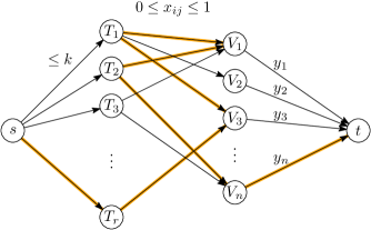
Figure 1: The network. The middle layer between the vertices $T_{i}$ and $V_{j}$ is a complete bipartite graph, but only a few selected arcs are shown. A potential augmenting path is highlighted.

There is now a one-to-one correspondence between integral flows from $s$ to $t$ in the network and solutions $(T_{1},\ldots,T_{r})$, and the cost of the flow is equal to the diversity (2) or (3). We are thus looking for a flow of maximum cost. The value of the flow (to total flow out of $s$) can be arbitrary. (It is equal to the sum of the sizes of the sets $T_{i}$.)

The concave arc costs (7) on the arcs leading to $t$ can be modeled in a standard way by multiple arcs. Denote the concave cost function by $f_{y}:=y(r-y)$, for $y=0,1,\ldots,r$. Then each arc $(V_{i},t)$ in the last layer is replaced by $r$ parallel arcs of capacity 1 with costs $f_{1}-f_{0}$, $f_{2}-f_{1}$, …, $f_{r}-f_{r-1}$. This sequence of values $f_{y}-f_{y-1}=r-2y+1$ is decreasing, starting out with positive values and ending with negative values. If the total flow along such a bundle is $y$, the maximum-cost way to distribute this flow is to fill the first $y$ arcs to capacity, for a total cost of $(f_{1}-f_{0})+(f_{2}-f_{1})+\dots+(f_{y}-f_{y-1})=f_{y}-f_{0}=f_{y}$, as desired.

An easy way to compute a maximum-cost flow is the longest augmenting path method. (Commonly it is presented as the shortest augmenting path method for the minimum-cost flow.) This holds for the classical flow model where the cost on each arc is a linear function of the flow. An augmenting path is a path in the residual network with respect to the current flow, and the cost coefficient of an arc in such a path must be taken with opposite sign if it is traversed in the direction opposite to the original graph.

Proposition 1 (The shortest augmenting path algorithm, cf. [32, Theorem 8.12]).

Suppose a maximum-cost flow among all flows of value $v$ from $s$ to $t$ is given. Let $P$ be a maximum-cost augmenting path from $s$ to $t$. If we augment the flow along this path, this results in a new flow, of some value $v^{\prime}$. Then the new flow is a maximum-cost flow among all flows of value $v^{\prime}$ from $s$ to $t$.

Let us apply this algorithm to our network. We initialize the constrained flow variables $x_{ij}$ according to (4) to 1 and all other variables $x_{ij}$ to 0. This corresponds to the original solution $(S_{1},S_{2},\ldots,S_{r})$, and it is clearly the optimal flow of value $\sum_{i=1}^{r}|S_{i}|$ because it is the only feasible flow of this value.

We can now start to find augmenting paths. Our graph is bipartite, and augmenting paths have a very simple structure: They start in $s$, alternate back and forth between the $T$-nodes and the $V$-nodes, and finally make a step to $t$. Moreover, in our network, all costs are zero except in the last layer, and an augmenting path contains precisely one arc from this layer. Therefore, the cost of an augmenting path is simply the cost of the final arc.

The flow variables in the final layer are never decreased. The resulting algorithm has therefore a simple greedy-like structure. Starting from the initial flow, we first try to saturate as many of the arcs of cost $f_{1}-f_{0}$ as possible. Next, we try to saturate as many of the arcs of cost $f_{2}-f_{1}$ as possible, and so on. Once the incremental cost $f_{y+1}-f_{y}$ becomes negative, we stop.

Trying to find an augmenting path whose last arc is one of the arcs of cost $f_{y+1}-f_{y}$, for fixed $y$, is a reachability problem in the residual graph, and it can be solved by graph search in $O(nr)$ time because the network has $O(nr)$ vertices. Every augmentation increases the flow value by 1 unit. Thus, there are at most $kr$ augmentations, for a total runtime of $O(kr^{2}n)$. ∎

3.2 Faster Augmentation

We can obtain faster algorithms by using more advanced network algorithms from the literature. We will derive one such algorithm here. The best choice depends on the relation between $n$, $k$, and $r$. We will apply the following result about $b$-matchings, which are generalizations of matchings: Each node $v$ has a given supply $b(v)$, specifying that $v$ should be incident to at most $v$ edges.

Proposition 2 ([1]).

A maximum-weight $b$-matching in a bipartite graph with $N_{1}+N_{2}$ nodes on the two sides of the bipartition and $M$ edges that have integer weights between $0$ and $W$ can be found in time $O(N_{1}M\log(2+\frac{{N_{1}\!}^{2}}{M}\log(N_{1}W)))$.

We will describe below how the network flow problem from above can be converted into a $b$-matching problem with $N_{1}=r+1$ plus $N_{2}=n$ nodes and $M=2rn$ edges of weight at most $W=2r$. Plugging these values into Proposition 2 gives a running time of $O(r^{2}n\log(2+\frac{r}{n}\log(r^{2})))=O(r^{2}n\max\{1,\log\frac{r\log r}{n}\})$ for finding an optimal augmentation. This improves over the run time $O(r^{2}nk)$ from the previous section unless $r$ is extremely large (at least $2^{k}$).

From the network of Figure 1, we keep the two layers of nodes $T_{i}$ and $V_{j}$. Each vertex $T_{i}$ gets a supply of $b(T_{i}):=k$, and each vertex $V_{j}$ gets a supply of $b(V_{j}):=r$. To mimic the piecewise linear costs on the arcs $(V_{j},t)$ in the original network, we introduce $r$ parallel slack edges from a new source vertex $s^{\prime}$ to each vertex $V_{i}$. The costs are as follows. Let $g_{1}>g_{2}>\cdots>g_{r}$ with $g_{y}=f_{y}-f_{y-1}$ denote the costs in the last layer of the original network, and let $\hat{g}:=r$. Since $g_{1}=r-1$, this is larger than all costs. Then every edge $(T_{i},V_{j})$ from the original network gets a weight of $\hat{g}$, and the $r$ new slack edges entering each $V_{j}$ get positive weights $\hat{g}-g_{1},\hat{g}-g_{2},\ldots,\hat{g}-g_{r}$. We set the supply of the extra source node to $b(s^{\prime}):=rn$, which imposes no constraint on the number of incident edges.

Now suppose that we have a solution for the original network in which the total flow into vertex $V_{j}$ is $y$. In the corresponding $b$-matching, we can then use $b(V_{j})-y$ = $r-y$ of the slack edges incident to $V_{j}$. The $r-y$ maximum-weight slack edges have weights $\hat{g}-g_{r},\hat{g}-g_{r-1},\ldots\hat{g}-g_{y+1}$. The total weight of the edges incident to $V_{j}$ is therefore

$$r\hat{g}-g_{r}-g_{r-1}-\cdots-g_{y+1}=r\hat{g}+(g_{1}+g_{2}+\cdots+g_{y}),$$

using the equation $g_{1}+g_{2}+\cdots+g_{r}=f_{r}-f_{0}=0$. Thus, up to an addition of the constant $nr\hat{g}$, the maximum weight of a $b$-matching agrees with the maximum cost of a flow in the original network.

3.3 Diverse Hitting Set

In this section we show how to use the optimal augmentation technique developed in Section 3 to solve Diverse $d$-Hitting Set. For this we use the following folklore lemma about minimal hitting sets.

Lemma 7.

Let $(U,\mathcal{F})$ be an instance of $d$-Hitting Set, and let $k$ be an integer. There are at most $d^{k}$ inclusion-minimal hitting sets of $\mathcal{F}$ of size at most $k$, and they can all be enumerated in time $d^{k}|U|^{2}$.

Combining Lemma 7 and Theorem 6, we obtain the following result.

Theorem 1.

Diverse $d$-Hitting Set can be solved in time $r^{2}d^{kr}\cdot|U|^{O(1)}$.

Proof.

Using Lemma 7, we can construct the set $\mathcal{S}$ of all inclusion-minimal hitting sets of $\mathcal{F}$, each of size at most $k$. Note that the size of $\mathcal{S}$ is bounded by $d^{k}$. As every superset of an element of $\mathcal{S}$ is also a hitting set, the theorem follows directly from Theorem 6. ∎

4 Diverse Feedback Vertex Set

A feedback vertex set (FVS) (also called a cycle cutset) of a graph $G$ is any subset $S\subseteq{}V(G)$ of vertices of $G$ such that every cycle in $G$ contains at least one vertex from $S$. The graph $G-S$ obtained by deleting $S$ from $G$ is thus an acyclic graph. Finding an FVS of small size is an NP-hard problem [20] with a number of applications in Artificial Intelligence, many of which stem from the fact that many hard problems become easy to solve in acyclic graphs. An example for this is the Propositional Model Counting (or #SAT) problem which asks for the number of satisfying assignments for a given CNF formula, and has a number of applications, for instance in planning [11, 27] and in probabilistic inference problems such as Bayesian reasoning [4, 23, 30, 2]. A popular approach to solving #SAT consists of first finding a small FVS $S$ of the CNF formula. Assigning values to all the variables in $S$ results in an acyclic instance of CNF. The algorithm assigns all possible sets of values to the variables in $S$, computes the number of satisfying assignments of the resulting acyclic instances, and returns the sum of these counts [10].

In this section, we focus on the Diverse Feedback Vertex Set problem and prove the following theorem.

Theorem 2.

Diverse Feedback Vertex Set can be solved in time $2^{7kr}\cdot n^{O(1)}$.

In order to solve $r$-Diverse $k$-Feedback Vertex Set, one natural way would be to generate every feedback vertex set of size at most $k$ and then check which set of $k$ solutions provide the required sum of Hamming distances. Unfortunately, the number of feedback vertex set is not $\mathsf{FPT}$ parameterized by $k$. Indeed, one can consider a graph containing $k$ cycle of size $\frac{n}{k}$, leading to $\left(\frac{n}{k}\right)^{k}$ different feedback vertex sets of size $k$.

We avoid this problem by generating all such small feedback vertex sets up to some equivalence of degree two vertices. We obtain an exact and efficient description of all feedback vertex sets of size at most $k$, which is formally captured by Lemma 8. A class of solutions of a graph $G$, is a pair $(S,\ell)$ such that $S\subseteq V(G)$ and $\ell:S\to 2^{V(G)}$ is a function such that for each $u\in S$, $u\in\ell(u)$, and for each $u,v\in S$, $u\not=v$, $\ell(u)\cap\ell(v)=\emptyset$. Given a class of solutions $(S,\ell)$, we define $\texttt{sol}(S,\ell)=\{S^{\prime}\subseteq V(G):|S^{\prime}|=|S|\text{ and }\forall v\in S,|S^{\prime}\cap\ell(v)|=1\}$. A class of FVS solutions is a class of solutions $(S,\ell)$ such that each $S^{\prime}\in\texttt{sol}(S,\ell)$ is a feedback vertex set of $G$. Moreover, if $S^{\prime}\in\texttt{sol}(S,\ell)$ and $S^{\prime}\subseteq S^{\prime\prime}\subseteq V(G)$, we say that $S^{\prime\prime}$ is described by $(S,\ell)$. Note that $S^{\prime\prime}$ is also a feedback vertex set. In a class of FVS solutions $(S,\ell)$, the meaning of the function $\ell$ is that, for each cycle $C$ in $G$, there exists $v\in S$ such that each element of $\ell(v)$ hits $C$. This allows us to group related solutions into only one set $\texttt{sol}(S,\ell)$.

Lemma 8.

Let $G$ be a $n$-vertex graph. There exists a set $\mathcal{S}$ of classes of FVS solutions of $G$ of size at most $2^{7k}$ such that each feedback vertex set of size at most $k$ is described by an element of $\mathcal{S}$. Moreover, $\mathcal{S}$ can be constructed in time $2^{7k}\cdot n^{O(1)}$.

Proof.

Let $G$ be a $n$-vertex graph. We start by generating a feedback vertex set $F\subseteq V$ of size at most $k$. The current best deterministic algorithm for this by Kociumaka and Pilipczuk [21] finds such a set in time $3.62^{k}\cdot n^{{O}(1)}$. In the following, we use the ideas used for the iterative compression approach [29].

For each subset $F^{\prime}\subseteq F$, we initiate a branching process by setting $A:=F^{\prime}$, $B:=F-F^{\prime}$, and $G^{\prime}:=G$. Observe that initially, as $B\subseteq F$ and $|F|\leq k$, the graph $G[B]$ has at most $k$ components. In the branching process, we will add more vertices to $A$ and $B$, and we will remove vertices and edges from $G^{\prime}$, but we will maintain the property that $A\subseteq V(G^{\prime})$ and $B\subseteq V(G^{\prime})$. The set $C$ will always denote the vertex set $V(G^{\prime})\setminus(A\cup B)$. Note that $G^{\prime}[C]$ is initially a forest; we ensure that it always remains a forest.

We also initialize a function $\ell\colon V(G)\to 2^{V(G)}$ by setting $\ell(v)=\{v\}$ for each $v\in V(G)$. This function will keep information about vertices that are deleted from $G$. While searching for a feedback vertex set, we consider only feedback vertex sets that contain all vertices of $A$ but no vertex of $B$. Vertices in $C$ are still undecided. The function $\ell$ will maintain the invariant that for each $v\in V(G^{\prime})$, $\ell(v)\cap V(G^{\prime})=\{v\}$, and for each $v\in C$, all vertices of $\ell(v)$ intersect exactly the same cycles in $G\setminus A$. Moreover, for each $v\in A$, the value $\ell(v)$ is fixed and will not be modified anymore in the branching process. During the branching process, we will progressively increase the size of $A$, $B$, and the sets $\ell(v)$, $v\in V(G)$.

By reducing $(G^{\prime},A,B,\ell)$ we mean that we apply the following rules exhaustively.

• If there is a $v\in C$ such that $\delta_{G^{\prime}[B\cup C]}(v)\leq 1$, we delete $v$ from $G^{\prime}$.

• If there is an edge $\{u,v\}\in E(G^{\prime}[C])$ such that $\delta_{G^{\prime}[B\cup C]}(u)=\delta_{G^{\prime}[B\cup C]}(v)=2$, we contract $u$ in $G^{\prime}$ and set $\ell(v):=\ell(v)\cup\ell(u)$.

These are classical preprocessing rules for the Feedback Vertex Set problem, see for instance [9, Section 9.1]. Indeed, vertices of degree one cannot appear in a cycle, and consecutive vertices of degree $2$ hit exactly the same cycles. After this preprocessing, there are no adjacent degree-two vertices and no degree-one vertices in $C$. (Degrees are measured in $G^{\prime}[B\cup C]$.)

We start to describe the branching procedure. We work on the tuple $(G^{\prime},A,B,\ell)$. After each step, the value $|A|-\texttt{cc}(B)$ will increase, where $\texttt{cc}(B)$ denotes the number of connected components of $G^{\prime}[B]$.

At each step of the branching we do the following. If $|A|>k$ or if $G^{\prime}[B]$ contains a cycle, we immediately stop this branch as there is no solution to be found in it. If $A$ is a feedback vertex set of size at most $k$, then $(A,\ell|_{A})$ is a class of FVS solutions, we add it to $\mathcal{S}$ and stop working on this branch. Otherwise, we reduce $(G^{\prime},A,B,\ell)$. We pick a deepest leaf $v$ in $G^{\prime}[C]$ and apply one of the two following cases, depending on the vertex $v$.

• Case 1: The vertex $v$ has at least two neighbors in $B$ (in the graph $G^{\prime}$).

  If there is a path in $B$ between two neighbors of $v$, then we have to put $v$ in $A$, as otherwise this path together with $v$ will induce a cycle. If there is no such path, we branch on both possibilities, inserting $v$ either into $A$ or into $B$.

• Case 2: The vertex $v$ has at most one neighbor in $B$.

  Since $v$ is a leaf in $G^{\prime}[C]$, it has at most one neighbor also in $C$. On the other hand, we know that $v$ has degree at least 2 in $G^{\prime}[B\cup C]$. Thus, $v$ has exactly one neighbor in $B$ and one neighbor in $C$, for a degree of $2$ in $G^{\prime}[B\cup C]$. Let $p$ be the neighbor in $C$. Again, as we have reduced $(G^{\prime},A,B,\ell)$, the degree of $p$ in $G^{\prime}[B\cup C]$ is at least $3$. So either it has a neighbor in $B$, or, as $v$ is a deepest leaf, it has another child, say $w$, that is also a leaf in $G^{\prime}[C]$, and $w$ has therefore a neighbor in $B$. We branch on the at most $2^{3}=8$ possibilities to allocate $v$, $p$, and $w$ if considered, between $A$ and $B$, taking care not to produce a cycle in $B$.

In both cases, either we put at least one vertex in $A$, and so $|A|$ increases by one, or all considered vertices are added to $B$. In the latter case, the considered vertices are connected, at least two of them have a neighbor in $B$, and no cycles were created; therefore, the number of components in $B$ drops by one. Thus $|A|-\texttt{cc}(B)$ increases by at least one. As $-k\leq|A|-\texttt{cc}(B)\leq k$, there can be at most $2k$ branching steps.

Since we branch at most $2k$ times and at each branch we have at most $2^{3}$ possibilities, the branching tree has at most $2^{6k}$ leaves. So, for each of the at most $2^{k}$ subsets $F^{\prime}$ of $F$, we add at most $2^{6k}$ elements to $\mathcal{S}$.

It is clear that we have obtained all solutions of FVS and they are described by the classes of FVS solutions in $\mathcal{S}$, which is of size $2^{7k}$. ∎

Proof of Theorem 2.

We generate all $2^{7kr}$ $r$-tuples of the classes of solutions given by Lemma 8, with repetition allowed.

We now consider each $r$-tuple $((S_{1},\ell_{1}),(S_{2},\ell_{2}),\ldots,(S_{r},\ell_{r}))\in\mathcal{S}^{r}$ and try to pick an appropriate solution $T_{i}$ from each class of solutions $(S_{i},\ell_{i})$, $i\in[1,k]$, in such a way that the diversity of the resulting tuple of feedback vertex sets $(T_{1},\ldots,T_{r})$ is maximized. The network of Section 3.1 must be adapted to model the constraints resulting from solution classes. Let $(S,\ell)$ be a solution class, with $|S|=b$. For our construction, we just need to know the family $\{\,\ell(v)\mid v\in S\,\}=\{L_{1},L_{2},\ldots,L_{b}\}$ of disjoint nonempty vertex sets. The solutions that are described by this class are all sets that can be obtained by picking at least one vertex from each set $L_{q}$. Figure 2 shows the necessary adaptations for one solution $T=T_{i}$. In addition to a single node $T$ that is either directly of indirectly connected to all nodes $V_{1},\ldots,V_{n}$, like in Figure 1, we have additional nodes representing the sets $L_{q}$. For each vertex $j$ that appears in one of the sets $L_{q}$, there is an additional node $U_{j}$ in an intermediate layer of the network. The flow from $s$ to $L_{q}$ is forced to be equal to 1, and this ensures that at least one element of the set $L_{q}$ is chosen in the solution. Here it is important that the sets $L_{q}$ are disjoint.

A similar structure must be built for each set $T_{1},\ldots,T_{r}$, and all these structures share the vertices $s$ and $V_{1},\ldots,V_{n}$. The rightmost layer of the network is the same as in Figure 1.

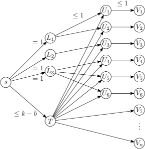
Figure 2: Part of the modified network for a solution $T$ which is specified by $b=3$ sets $L_{1}=\{1,2\},L_{2}=\{3\}$, and $L_{3}=\{4,5,6\}$.

The initial flow is not so straightforward as in Section 3.1 but is still easy to find. We simply saturate the arc from $s$ to each of the nodes $L_{q}$ in turn by a shortest augmenting path. Such a path can be found by a simple reachability search in the residual network, in $O(rn)$ time. The total running time $O(kr^{2}n)$ from Section 3.1 remains unchanged. ∎

5 Modeling Aspects: Discussion of the Objective Function

In Sections 3 and 4, we have used the sum of the Hamming distances, $\textrm{div}_{\mathrm{total}}$, as the measure of diversity. While this metric is of natural interest, it appears that in some specific cases, it may not be a useful choice. We present a simple example where the most diverse solution according to $\textrm{div}_{\mathrm{total}}$ is not what one might expect.

Let $r$ be an even number. We consider the path with $2r-2$ vertices, and we are looking for $r$ vertex covers of size at most $r-1$, of maximum diversity.

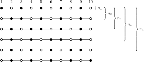
Figure 3: The $r=6$ different vertex covers of size $r-1=5$ in a path with $2(r-1)=10$ vertices

Figure 3 shows an example with $r=6$. The smallest size of a vertex cover is indeed $r-1$, and there are $r$ different solutions. One would hope that the “maximally diverse” selection of $r$ solutions would pick all these different solutions. But no, the selection that maximizes $\textrm{div}_{\mathrm{total}}$ consists of $r/2$ copies of just two solutions, the “odd” vertices and the “even” vertices (the first and last solution in Figure 3).

This can be seen as follows. If the selected set contains in total $n_{i}$ copies of the first $i$ solutions in the order of Figure 3, then the objective can be written as

$$2n_{1}(r-n_{1})+2n_{2}(r-n_{2})+\cdots+2n_{r-1}(r-n_{r-1}).$$

Here, each term $2n_{i}(r-n_{i})$ accounts for two consecutive vertices $2i-1,2i$ of the path in the formulation (3). The unique way of maximizing each term individually is to set $n_{i}=r/2$ for all $i$. This corresponds to the selection of $r/2$ copies of the first solution and $r/2$ copies of the last solution, as claimed.

In a different setting, namely the distribution of $r$ points inside a square, an analogous phenomenon has been observed [33, Figure 1]: Maximizing the sum of pairwise Euclidean distances places all points at the corners of the square. In fact it is easy to see that, in this geometric setting, any locally optimal solution must place all points on the boundary of the feasible region. By contrast, for our combinatorial problem, we don’t know whether this pathological behavior is typical or rare in instances that are not specially constructed. Further research is needed. A notion of diversity which is more robust in this respect is the smallest difference between two solutions, which we consider in Section 6.

6 Maximizing the Smallest Hamming distance

The undesired behavior highlighted in Section 5 is the fact that the collection that maximizes the sum of the Hamming distances uses several copies of the same set. In this section we explore how to handle this unexpected behavior by changing the distance to the minimal Hamming distance between two sets of the collection. This modification naturally removes the possibility of selecting the same solution twice. We show how to solve Min-Diverse $d$-Hitting Set and $r$-Min-Diverse $k$-Feedback Vertex Set for this metric.

Theorem 3.

Min-Diverse $d$-Hitting Set can be solved in time

• $2^{kr^{2}}\cdot(kr)^{O(1)}$ if $|U|<kr$ and

• $d^{kr}\cdot|U|^{O(1)}$ otherwise.

Proof.

Let $(U,\mathcal{F},k,r,t)$ be an instance of Min-Diverse $d$-Hitting Set where $|U|=n$. If $n<kr$, we solve the problem by complete enumeration: There are trivially at most $2^{n}$ hitting sets of size at most $k$. We form all $r$-tuples $(T_{1},\ldots,T_{r})$ of them and select the one that maximizes $\textrm{div}_{\mathrm{min}}(T_{1},\ldots,T_{r})$. The running time is at most $O((2^{n})^{r}r^{2}n)=O(2^{kr^{2}}kr^{3})$.

We now assume that $n\geq kr$. We use the same strategy as in Section 3: We generate all $r$-tuples $(S_{1},\ldots,S_{r})$ of minimal solutions and try to augment each one to a $r$-tuple $(T_{1},\ldots,T_{r})$ such that for each $i\in[1,r]$, $|T_{i}|\leq k$ and $S_{i}\subseteq T_{i}\subseteq V(G)$ hold. The difference is that we try to maximize $\textrm{div}_{\mathrm{min}}(T_{1},\ldots,T_{r})$ instead of $\textrm{div}_{\mathrm{total}}(T_{1},\ldots,T_{r})$ in the augmentation. Given that we have a large supply of $n\geq kr$ elements in $U$, this is easy. To each set $S_{i}$ we add $k-|S_{i}|$ new elements, taking care that we pick different elements for each $S_{i}$ with are not in any of the other sets $S_{j}$. The Hamming distance between two resulting sets is then $d_{H}(T_{i},T_{j})=d_{H}(S_{i},S_{j})+(k-|S_{i}|)+(k-|S_{i}|)$, and it is clear that this is the largest possibly distance that two sets $T^{\prime}_{i}\supseteq S_{i}$ and $T^{\prime}_{j}\supseteq S_{j}$ with $|T^{\prime}_{i}|,|T^{\prime}_{j}|\leq k$ can achieve. Thus, since our choice of augmentation individually maximizes each pairwise Hamming distance, it also maximizes the smallest Hamming distance. This procedure can be carried out in $O(kr+n)=O(n)$ time. In addition, we need $O(kr^{2})=O(n^{2})$ time to compute the smallest distance.

Using Lemma 7, we construct the set $\mathcal{S}$ of all minimal solutions of the $d$-Hitting Set instance $(U,\mathcal{F})$, each of size at most $k$. We then go through every $r$-tuple $(S_{1},\ldots,S_{r})\in\mathcal{S}^{r}$ and augment it optimally, as just described. The running time is $d^{kr}\cdot O(n^{2})$. ∎

Theorem 4.

Min-Diverse Feedback Vertex Set can be solved in time $2^{kr\cdot\max(r,7+\log_{2}(kr))}\cdot(nr)^{O(1)}$.

Proof.

Let $G$ be a $n$-vertex graph. If $n<kr$, we again solve the problem by complete enumeration: There are trivially at most $2^{n}$ feedback vertex sets of size at most $k$. We form all $r$-tuples $(T_{1},\ldots,T_{r})$ of them and select the one that maximizes $\textrm{div}_{\mathrm{min}}(T_{1},\ldots,T_{r})$. The running time is at most $O((2^{n})^{r}r^{2}n)=O(2^{kr^{2}}r^{2}n)$.

We assume now that $n\geq kr$. As in Section 4, we construct a set $\mathcal{S}$ of at most $2^{7k}$ classes of FVS solutions of $G$, using Lemma 8. Then we go through all $(2^{7k})^{r}$ $r$-tuples of classes $S=((S_{1},\ell_{1}),\ldots,(S_{r},\ell_{r}))\in\mathcal{S}^{r}$. For each such $r$-tuple, we look for the $r$-tuple $(T_{1},\ldots,T_{r})$ of feedback vertex sets such that each $T_{i}$ is described by $(S_{i},\ell_{i})$, and the objective value $\textrm{div}_{\mathrm{min}}(T_{1},\ldots,T_{r})$ is maximized. So far, the procedure is completely analogous to the algorithm of Theorem 2 in Section 4 for maximizing $\textrm{div}_{\mathrm{total}}(T_{1},\ldots,T_{r})$.

Now, in going from a class $(S_{i},\ell_{i})$ to $T_{i}$, we have to select a vertex from every set $\ell_{i}(v)$, for $v\in S_{i}$, and we may add an arbitrary number of additional vertices, up to size $k$. We make this selection as follows: Whenever $|\ell_{i}(v)|<kr$, we simply try all possibilities of choosing an element of $\ell_{i}(v)$ and putting it into $T_{i}$. If $|\ell_{i}(v)|\geq kr$, we defer the choice for later. In this way, we have created at most $(kr)^{kr}$ “partial” feedback vertex sets $(T^{0}_{1},\ldots,T^{0}_{r})$

For each such $(T^{0}_{1},\ldots,T^{0}_{r})$, we now add the remaining elements. In each list $\ell_{i}(v)$ which has been deferred, we greedily pick an element that is distinct from all other chosen elements. This is always possible since the list is large enough. Finally, we fill up the sets to size $k$, again choosing fresh elements each time. Each such choice is an optimal choice, because it increases the Hamming distance between the concerned set $T_{i}$ and every other set $T_{j}$ by 1, which is the best that one can hope for. As we proceed to this operation for each $S\in\mathcal{S}^{r}$, where $|\mathcal{S}|\leq 2^{7k}$, and that for each such $S$, we create at most $(kr)^{kr}$ $r$-tuples, we obtain an algorithm running in time $2^{7kr}\cdot(kr)^{kr}\cdot n^{O(1)}$. The theorem follows. ∎

7 Conclusions and Open Problems

In this work, we have considered the paradigm of finding small diverse collections of reasonably good solutions to combinatorial problems, which has recently been introduced to the field of fixed-parameter tractability theory [5].

We have shown that finding diverse collections of $d$-hitting sets and feedback vertex sets can be done in $\mathsf{FPT}$ time. While these problems can be classified as $\mathsf{FPT}$ via the kernels and a treewidth-based meta-theorem proved in [5], the methods proposed here are of independent interest. We introduced a method of generating a maximally diverse set of solutions from a set that either contains all minimal solutions of bounded size ($d$-Hitting Set) or from a collection of structures that in some way describes all solutions of bounded size (Feedback Vertex Set). In both cases, the maximally diverse collection of solutions is obtained via a network flow model, which does not rely on any specific properties of the studied problems. It would be interesting to see if this strategy can be applied to give FPT-algorithms for diverse problems that are not covered by the meta-theorem or the kernels presented in [5].

While the problems in [5] as well as the ones in Sections 3 and 4, seek to maximize the sum of all pairwise Hamming distances, we also studied the variant that asks to maximize the minimum Hamming distance, taken over each pair of solutions. This was motivated by an example where the former measure does not perform as intended (Section 5). We showed that also under this objective, the diverse variants of $d$-Hitting Set and Feedback Vertex Set are $\mathsf{FPT}$. It would be interesting to see whether this objective also allows for a (possibly treewidth-based) meta-theorem.

In [5], the authors ask whether there is a problem that is in $\mathsf{FPT}$ parameterized by solution size whose $r$-diverse variant becomes $\mathsf{W[1]}$-hard upon adding $r$ as another component of the parameter. We restate this question here.

Open Question ([5]).

Is there a problem $\Pi$ with solution size $k$, such that $\Pi$ is $\mathsf{FPT}$ parameterized by $k$, while Diverse $\Pi$, asking for $r$ solutions, is $\mathsf{W[1]}$-hard parameterized by $k+r$?

To the best of our knowledge, this problem is still wide open. We believe that the $\textrm{div}_{\mathrm{min}}$ measure is more promising to obtain such a result rather than the $\textrm{div}_{\mathrm{total}}$ measure. A possible way to tackle both measures at once might be a parameterized (and strenghtened) analogue of the following approach that is well-studied in classical complexity. Yato and Seta propose a framework [36] to prove $\mathsf{NP}$-completeness of finding a second solution to an $\mathsf{NP}$-complete problem. In other words, there are some problems where given one solution it is still $\mathsf{NP}$-hard to determine whether the problem has a different solution.

From a different perspective, one might want to identify problems where obtaining one solution is polynomial-time solvable, but finding a diverse collection of $r$ solutions becomes $\mathsf{NP}$-hard. The targeted running time should be $\mathsf{FPT}$ parameterized by $r$ (and maybe $t$, the diversity target) only. We conjecture that this is most probably $\mathsf{NP}$- or $\mathsf{W[-]}$ hard in general. However, we believe it is interesting to search for well-known problems where it is not the case.

Acknowledgments.

The first, second, third and fourth authors would like to thank Mike Fellows for introducing them to the notion of diverse $\mathsf{FPT}$ algorithms and sharing the manuscript “The Diverse $X$ Paradigm” [13].

References

- [1] Ravindra K. Ahuja, James B. Orlin, Clifford Stein, and Robert E. Tarjan. Improved algorithms for bipartite network flow. SIAM Journal on Computing, 23:906–933, 1994. doi:10.1137/S0097539791199334.
- [2] Udi Apsel and Ronen I. Brafman. Lifted MEU by weighted model counting. In Proceedings of the Twenty-Sixth AAAI Conference on Artificial Intelligence, pages 1861–1867. AAAI Press, 2012.
- [3] Marcelo Arenas, Leopoldo Bertossi, Jan Chomicki, Xin He, Vijay Raghavan, and Jeremy Spinrad. Scalar aggregation in inconsistent databases. Theoretical Computer Science, 296(3):405–434, 2003. doi:10.1016/S0304-3975(02)00737-5.
- [4] Fahiem Bacchus, Shannon Dalmao, and Toniann Pitassi. Algorithms and complexity results for #SAT and Bayesian inference. In Proceedings of the 44th Annual IEEE Symposium on Foundations of Computer Science, pages 340–351. IEEE, 2003. doi:10.1109/SFCS.2003.1238208.
- [5] Julien Baste, Michael R. Fellows, Lars Jaffke, Tomáš Masařík, Mateus de Oliveira Oliveira, Geevarghese Philip, and Frances A. Rosamond. Diversity in combinatorial optimization. CoRR, 2019. arXiv:1903.07410.
- [6] Julien Baste, Lars Jaffke, Tomáš Masařík, Geevarghese Philip, and Günter Rote. Fpt algorithms for diverse collections of hitting sets. Algorithms, 12(12), 2019. doi:10.3390/a12120254.
- [7] Karl Bringmann, Sergio Cabello, and Michael T. M. Emmerich. Maximum volume subset selection for anchored boxes. In Boris Aronov and Matthew J. Katz, editors, 33rd International Symposium on Computational Geometry (SoCG 2017), volume 77 of Leibniz International Proceedings in Informatics (LIPIcs), pages 22:1–22:15, Dagstuhl, Germany, 2017. Schloss Dagstuhl–Leibniz-Zentrum für Informatik. doi:10.4230/LIPIcs.SoCG.2017.22.
- [8] Jan Chomicki and Jerzy Marcinkowski. Minimal-change integrity maintenance using tuple deletions. Information and Computation, 197(1–2):90–121, 2005. doi:10.1016/j.ic.2004.04.007.
- [9] Marek Cygan, Fedor V. Fomin, Lukasz Kowalik, Daniel Lokshtanov, Dániel Marx, Marcin Pilipczuk, Michal Pilipczuk, and Saket Saurabh. Parameterized Algorithms. Springer, 2015. doi:10.1007/978-3-319-21275-3.
- [10] Rina Dechter and David Cohen. Constraint Processing. Morgan Kaufmann, 2003.
- [11] Carmel Domshlak and Jörg Hoffmann. Fast probabilistic planning through weighted model counting. In Proceedings of the Sixteenth International Conference on Automated Planning and Scheduling, ICAPS 2006, pages 243–252. AAAI Press, 2006.
- [12] Matthias Ehrgott. Multicriteria Optimization, volume 491 of LNE. Springer, 2005.
- [13] Michael Ralph Fellows. The diverse X paradigm. Manuscript, November 2018.
- [14] Thomas Gabor, Lenz Belzner, Thomy Phan, and Kyrill Schmid. Preparing for the unexpected: Diversity improves planning resilience in evolutionary algorithms. In 2018 IEEE International Conference on Autonomic Computing, ICAC 2018, Trento, Italy, September 3-7, 2018, pages 131–140, 2018. doi:10.1109/ICAC.2018.00023.
- [15] Per Galle. Branch & sample: A simple strategy for constraint satisfaction. BIT Numerical Mathematics, 29(3):395–408, 1989. doi:10.1007/BF02219227.
- [16] Sorabh Gandhi, Chiranjeeb Buragohain, Lili Cao, Haitao Zheng, and Subhash Suri. A general framework for wireless spectrum auctions. In Proceedings 2nd IEEE International Symposium on New Frontiers in Dynamic Spectrum Access Networks, pages 22–33. IEEE, 2007.
- [17] Martin Hoefer, Thomas Kesselheim, and Berthold Vöcking. Approximation algorithms for secondary spectrum auctions. ACM Transactions on Internet Technology (TOIT), 14(2–3):16:1–16:24, 2014. doi:10.1145/2663496.
- [18] M. Idan, G. Iosilevskii, and L. Ben-Yishay. Efficient air traffic conflict resolution by minimizing the number of affected aircraft. International Journal of Adaptive Control and Signal Processing, 24(10):867–881, 2010.
- [19] Ekaterini Ioannou and Slawek Staworko. Management of inconsistencies in data integration. In Data Exchange, Integration, and Streams, volume 5, pages 217–225. Schloss Dagstuhl-Leibniz-Zentrum für Informatik, 2013. doi:10.4230/DFU.Vol5.10452.217.
- [20] Richard M Karp. Reducibility among combinatorial problems. In Complexity of Computer Computations, pages 85–103. Springer, 1972.
- [21] Tomasz Kociumaka and Marcin Pilipczuk. Faster deterministic feedback vertex set. Information Processing Letters, 114(10):556–560, 2014. doi:10.1016/j.ipl.2014.05.001.
- [22] Tobias Kuhn, Carlos M. Fonseca, Luís Paquete, Stefan Ruzika, Miguel M. Duarte, and José Rui Figueira. Hypervolume subset selection in two dimensions: Formulations and algorithms. Evolutionary Computation, 24(3):411–425, 2016. doi:10.1162/EVCO_a_00157.
- [23] Michael L. Littman, Stephen M. Majercik, and Toniann Pitassi. Stochastic Boolean satisfiability. Journal of Automated Reasoning, 27(3):251–296, 2001. doi:10.1023/A:1017584715408.
- [24] Sushil J. Louis and Gregory J. E. Rawlins. Syntactic analysis of convergence in genetic algorithms. In Proceedings of the Second Workshop on Foundations of Genetic Algorithms. Vail, Colorado, USA, July 26-29 1992., pages 141–151, 1992. doi:10.1016/b978-0-08-094832-4.50015-5.
- [25] Ronald W. Morrison and Kenneth A. De Jong. Measurement of population diversity. In Artificial Evolution, 5th International Conference, Evolution Artificielle, EA 2001, Le Creusot, France, October 29-31, 2001, Selected Papers, pages 31–41, 2001. doi:10.1007/3-540-46033-0\_3.
- [26] Aneta Neumann, Wanru Gao, Carola Doerr, Frank Neumann, and Markus Wagner. Discrepancy-based evolutionary diversity optimization. In Proceedings of the Genetic and Evolutionary Computation Conference, GECCO ’18, pages 991–998, New York, NY, USA, 2018. ACM. doi:10.1145/3205455.3205532.
- [27] Héctor Palacios, Blai Bonet, Adnan Darwiche, and Héctor Geffner. Pruning conformant plans by counting models on compiled d-DNNF representations. In Proceedings of the Fifteenth International Conference on Automated Planning and Scheduling, ICAPS 2005, pages 141–150. AAAI Press, 2005.
- [28] Enela Pema, Phokion G. Kolaitis, and Wang-Chiew Tan. On the tractability and intractability of consistent conjunctive query answering. In Proceedings of the 2011 Joint EDBT/ICDT Ph. D. Workshop, pages 38–44. ACM, 2011. doi:10.1145/1966874.1966881.
- [29] Bruce Reed, Kaleigh Smith, and Adrian Vetta. Finding odd cycle transversals. Operations Research Letters, 32(4):299–301, 2004. doi:10.1016/j.orl.2003.10.009.
- [30] Tian Sang, Paul Bearne, and Henry Kautz. Performing Bayesian inference by weighted model counting. In Proceedings of the 20th National Conference on Artificial Intelligence-Volume 1, pages 475–481. AAAI Press, 2005.
- [31] Andrew R. Solow and Stephen Polasky. Measuring biological diversity. Environmental and Ecological Statistics, 1(2):95–103, Jun 1994. doi:10.1007/BF02426650.
- [32] Robert E. Tarjan. Data Structures and Network Algorithms. SIAM, Philadelpia, 1983. doi:10.1137/1.9781611970265.
- [33] Tamara Ulrich, Johannes Bader, and Lothar Thiele. Defining and optimizing indicator-based diversity measures in multiobjective search. In Robert Schaefer, Carlos Cotta, Joanna Kołodziej, and Günter Rudolph, editors, Parallel Problem Solving from Nature, PPSN XI, pages 707–717, Berlin, Heidelberg, 2010. Springer. doi:10.1007/978-3-642-15844-5_71.
- [34] Adan Ernesto Vela. Understanding conflict-resolution taskload: implementing advisory conflict-detection and resolution algorithms in an airspace. PhD thesis, Georgia Institute of Technology, 2011.
- [35] Mark Wineberg and Franz Oppacher. The underlying similarity of diversity measures used in evolutionary computation. In Genetic and Evolutionary Computation - GECCO 2003, Genetic and Evolutionary Computation Conference, Chicago, IL, USA, July 12-16, 2003. Proceedings, Part II, pages 1493–1504, 2003. doi:10.1007/3-540-45110-2\_21.
- [36] Takayuki Yato and Takahiro Seta. Complexity and completeness of finding another solution and its application to puzzles. IEICE transactions on fundamentals of electronics, communications and computer sciences, 86(5):1052–1060, 2003.