$0$–$1$ phase transitions in sparse spiked matrix estimation

Abstract

We consider statistical models of estimation of a rank-one matrix (the spike) corrupted by an additive gaussian noise matrix in the sparse limit. In this limit the underlying hidden vector (that constructs the rank-one matrix) has a number of non-zero components that scales sub-linearly with the total dimension of the vector, and the signal strength tends to infinity at an appropriate speed. We prove explicit low-dimensional variational formulas for the asymptotic mutual information between the spike and the observed noisy matrix in suitable sparse limits. For Bernoulli and Bernoulli-Rademacher distributed vectors, and when the sparsity and signal strength satisfy an appropriate scaling relation, these formulas imply sharp $0$–$1$ phase transitions for the asymptotic minimum mean-square-error. A similar phase transition was analyzed recently in the context of sparse high-dimensional linear regression (compressive sensing) [1, 2].

1  Introduction

Low rank matrix estimation (or factorization) is an important problem with numerous applications in image processing, principal component analysis (PCA), machine learning, DNA microarray data, tensor decompositions, etc. These modern applications often require to look at the high-dimensional limit and sparse limits of the problem. Sparsity is often a crucial ingredient for the interpretability of high dimensional statistical models. In this context, it is of great importance to determine computational limits of estimation and to benchmark them by the fundamental information theoretical (i.e., statistical) limits. In this paper we concentrate on information theoretic limits for two probabilistic models, the so-called sparse spiked Wishart and Wigner matrix models.

In the simplest rank-one version one seeks a matrix ${\bm{U}}\otimes{\bm{V}}$ constructed from high-dimensional hidden vectors ${\bm{U}}=(U_{1},\ldots,U_{n})\in\mathbb{R}^{n}$ and ${\bm{V}}=(V_{1},\ldots,V_{m})\in\mathbb{R}^{m}$, $m=\alpha_{n}n$, based on a noisy observed data matrix ${\bm{W}}$ with entries obtained as $W_{ij}\sim{\cal N}(\sqrt{\lambda_{n}/n}\,U_{i}V_{j},1)$ for $i=1,\dots,n$, $j=1,\dots,m$ and $\lambda_{n}>0$ the signal strength. The hidden vectors have independent identically distributed (i.i.d.) components drawn from two different distributions. The high-dimensional limit means that we look at $n,m\to+\infty$, $\alpha_{n}\to\alpha>0$. We suppose that ${\bm{V}}$ has on average $\rho_{V,n}m$ non-zero component which scales sub-linearly for a sequence $\rho_{V,n}\to 0_{+}$. We will see that non-trivial estimation is only possible if $\lambda_{n}\to+\infty$ (whereas if $\rho_{V,n}\to\rho_{V}>0$, $\lambda_{n}\to\lambda>0$ finite). The problem is to estimate ${\bm{U}}\otimes{\bm{V}}$ given the data matrix ${\bm{W}}$. In the Bayesian setting, which is our concern here, it is supposed that the priors and hyper-parameters are all known. We will refer to this problem as the sparse spiked Wishart matrix model.

A popular version of this model, and one addressed here, corresponds to a fixed standard gaussian distribution for ${\bm{U}}\sim\mathcal{N}(0,{\rm I}_{n})$ (${\rm I}_{n}$ is the $n\times n$ identity matrix) and a Bernoulli-Rademacher distribution for $V_{i}\sim P_{V,n}=(1-\rho_{V,n})\delta_{0}+\frac{1}{2}\rho_{V,n}(\delta_{-1}+\delta_{1})$. This estimation problem is equivalent to the important “spiked covariance model” or “gaussian sparse-PCA” [3, 4] which amounts to estimate a sparse binary matrix ${\bm{V}}\otimes{\bm{V}}$ from samples generated by the normal law $\mathcal{N}(0,{\rm I}_{n}+\frac{\lambda}{n}{\bm{V}}\otimes{\bm{V}})$.

An even simpler and paradigmatic matrix estimation problem has a symmetric data matrix ${\bm{W}}$ with elements drawn as $W_{ij}\sim{\cal N}(\sqrt{\lambda_{n}/n}\,X_{i}X_{j},1)$ for $1\leq i<j\leq n$ and ${\bm{X}}=(X_{1},\dots,X_{n})\in\mathbb{R}^{n}$ with i.i.d. components, with $n\to+\infty$ in the high-dimensional limit. Again, the sparse version corresponds to having a sub-linear number of non-zero components, i.e., $\rho_{n}n$ with $\rho_{n}\to 0_{+}$, and non-trivial estimation is possible only for $\lambda_{n}\to+\infty$. We call this model the sparse spiked Wigner matrix model. We will focus in particular on binary vectors generated from Bernoulli $X_{i}\sim P_{X,n}={\rm Ber}(\rho_{n})$ or Bernoulli-Rademacher $X_{i}\sim P_{X,n}=(1-\rho_{n})\delta_{0}+\frac{1}{2}\rho_{n}(\delta_{-1}+\delta_{1})$ distributions.

1.1 Background

Much progress has been accomplished in recent years on spiked matrix models for non-sparse settings, by which we mean that the distributions $P_{X}$, $P_{U}$, $P_{V}$ are fixed independent of $n,m$, and thus the number of non-zero components of ${\bm{X}}$, ${\bm{V}}$, even if “small”, scales linearly with $n$. An interesting phenomenology of information theoretical (or statistical) as well as computational limits has been derived [5] by heuristic methods of statistical physics of spin glass theory (the so-called replica method). In the asymptotic regime of $n\!\to\!+\infty$ these limits take the form of sharp phase transitions. The rigorous mathematical theory of these phase transitions is now largely under control. On one hand, the approximate message passing (AMP) algorithm has been analyzed by state evolution [6, 7]. And on the other hand, the asymptotic mutual informations per variable between hidden spike and data matrices, have been rigorously computed in a series of works using various methods (cavity method, spatial coupling, interpolation methods) [8, 9, 10, 11, 12, 13, 14, 15, 16, 17, 18]. The information theoretic phase transitions are then signalled by singularities, as a function of the signal strength, in the limit of the mutual information per variable when $n\to+\infty$. The phase transition also manifests itself as a jump discontinuity in the minimum mean-square-error (MMSE). Once the mutual information is known it is usually possible to deduce the MMSE. For example, in the simplest case of the spiked Wigner model, if $I({\bm{X}}\otimes{\bm{X}};{\bm{W}})$ is the mutual information between the spike ${\bm{X}}\otimes{\bm{X}}$ and the data ${\bm{W}}$, the ${\rm MMSE}({\bm{X}}\otimes{\bm{X}}|{\bm{W}})=\mathbb{E}\|{\bm{X}}\otimes{\bm{X}}-\mathbb{E}[{\bm{X}}\otimes{\bm{X}}|{\bm{W}}]\|_{\rm F}^{2}$ satisfies the I-MMSE relation (such relations are derived in [19, 20], see also appendix 11)

$$\frac{d}{d\lambda_{n}}\frac{1}{n}I({\bm{X}}\otimes{\bm{X}};{\bm{W}})=\frac{1}{4n^{2}}{\rm MMSE}({\bm{X}}\otimes{\bm{X}}|{\bm{W}})+O(n^{-1})\,.$$

Closed form expressions for the asymptotic mutual information [11, 12, 10, 13, 14, 15] therefore allow to benchmark the fundamental information theoretical limits of estimation. See also [21, 22, 23] for results on the limits of detecting the precense of a spike in a noisy matrix, rather than estimating it.

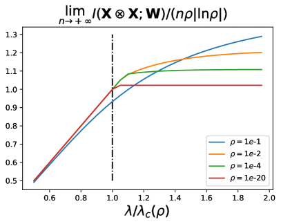
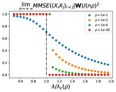
Figure 1: A sequence of suitably normalized mutual information and minimum mean-square-error (MMSE) curves as a function of $\lambda/\lambda_{c}(\rho)$ for the symmetric matrix estimation model for $X_{i}\sim{\rm Ber}(\rho)$. Here $\lambda_{c}(\rho)=4|\ln\rho|/\rho$. In the sparse limit $\rho\to 0$ the MMSE curves approach a $0$–$1$ phase transition with the discontinuity at $\lambda=\lambda_{c}(\rho)$. This corresponds to an angular point for the mutual information.

1.2 Our contributions

In this paper we are exclusively interested in determining information theoretic phase transitions in regimes of sub-linear sparsity. We identify the correct scaling regimes of vanishing sparsity and diverging signal strength in which non-trivial information theoretic phase transitions occur. We use the adaptive interpolation method [13, 14, 15] first introduced in the non-sparse matrix estimation problems, to provide for the sparse limit, closed form expressions of the mutual information in terms of low-dimensional variational expressions (theorems 1 and 4 in section 2). That the adaptive interpolation method can be extended to the sparse limit is interesting and not a priori obvious. By the I-MMSE relation and the solution of the variational problems we then find, for Bernoulli and Bernoulli-Rademacher distributions of the sparse signal, that the MMSE displays to a $0$–$1$ phase transition and we determine the exact thresholds.

Let us describe the regimes studied and the information theoretical thresholds found here (precise statements are found in section 2). We first note that for sub-linear sparsity, a phase transition appears only if the signal strength tends to infinity. For the Wigner case, for example, this can be seen from the following heuristic argument: the total signal-to-noise ratio (SNR) per non-zero component (i.e., SNR per observation $(\lambda_{n}/n)\rho_{n}^{2}$ times the number of observations $\Theta(n^{2})$ divided by the number of non-zero components $\rho_{n}n$) scales as $(\lambda_{n}/n)\rho_{n}^{2}n^{2}/(\rho_{n}n)=\lambda_{n}\rho_{n}$ so that $\lambda_{n}\to+\infty$ is necessary in order to have enough energy to estimate the non-zero components. Our analysis shows that non-trivial phase transitions occur when $\lambda_{n}=\Theta(|\ln\rho_{n}|/\rho_{n})$ (Wigner case) and $\lambda_{n}=\Theta(\sqrt{|\ln\rho_{V,n}|/\rho_{V,n}})$ (Wishart case) when $\rho_{n}$ and $\rho_{V,n}$ tend to zero slowly enough.

We study in particular the cases of binary signals, i.e., $P_{X,n}$ and $P_{V,n}$ equal to ${\rm Ber}(\rho_{n})$ or Bernoulli-Rademacher $(1-\rho_{n})\delta_{0}+\frac{1}{2}\rho_{n}(\delta_{-1}+\delta_{1})$. For these distributions we find $0$–$1$ phase transitions at the level of the MMSE as long as $\rho_{n}\to 0_{+}$ and $\rho_{V,n}\to 0_{+}$ not too fast. This is illustrated on figure 1 for the Wigner case with Bernoulli distribution. The left hand side shows that as $\rho_{n}\to 0_{+}$ the (suitably normalized) mutual information approaches the broken line with an angular point at $\lambda/\lambda_{c}(\rho_{n})=1$ where $\lambda_{c}(\rho_{n})=4|\ln\rho_{n}|/\rho_{n}$; in the case of Bernoulli-Rademacher distribution the threshold is the same. On the right hand side the (suitably normalized) MMSE approaches a $0$–$1$ curve: it tends to $1$ for $\lambda/\lambda_{c}(\rho_{n})<1$, develops a jump discontinuity at $\lambda/\lambda_{c}(\rho_{n})=1$, and takes the value $0$ when $\lambda/\lambda_{c}(\rho_{n})>1$. A similar $0$–$1$ transition is found to hold for the MMSE of ${\bm{V}}\otimes{\bm{V}}$ in the spiked covariance model with a threshold $\lambda_{c}(\rho_{V,n})=\sqrt{4|\ln\rho_{n}|/(\alpha_{n}\rho_{n})}$ (with $\alpha_{n}\to\alpha$). This is illustrated on figure 2 in section 2. Note that these figures are obtained from the asymptotic prediction where first $n\to+\infty$ and then $\rho\to 0_{+}$, so not in the sub-linear sparsity regime. Our analysis confirms that this picture with its sharp transition holds in the truly sparse (sub-linear) regime $\rho_{n}\to 0_{+}$ with $n\to+\infty$.

1.3 Related work

Spiked matrix ensembles have played a crucial role in the analysis of threshold phenomena in high-dimensional statistical models for almost two decades. Early rigorous results are found in [24] who determined by spectral methods the location of the information theoretic phase transition point in a spiked covariance model, and [25, 26] for the Wigner case. More recently, the information theoretic limits and those of hypothesis testing have been derived, with the additional structure of sparse vectors, for large but finite sizes [27, 28, 29]. These estimates are consistent with our results. The additional feature that we provide here, is an asymptotic limit in which a sharp $0$–$1$ phase transition is identified, with fully explicit formulas for the thresholds. Moreover closed form expressions for the mutual information are also determined.

The $0$–$1$ transitions and formulas for the thresholds and mutual information were first computed in [5] using the heuristic replica method of spin-glass theory. However, it must be stressed that, not only this calculation is far from rigorous, but more importantly the limit $n\!\to\!+\infty$ is first taken for fixed parameters $\rho_{n}\!=\!\rho$, $\rho_{V,n}\!=\!\rho_{V}$, and the sparse limit $\rho,\rho_{V}\!\to\!0_{+}$ is taken only after. Although the thresholds found in this way agree with our derivation of $\lambda_{c}(\rho_{n})$, this is far from evident a priori. For example, it not clear if this sort of approach yields correct computational thresholds in the sparse limit [30, 5].

Similar phase transitions in sublinear sparse regimes for binary signals (Bernoulli or Bernoulli-Rademacher) have been studied in the context of linear estimation or compressed sensing [1, 2] for support recovery. These works focus on the MMSE and prove the occurence of the $0$–$1$ phase transition which they call an “all-or-nothing” phenomenon. We note that our approach is technically very different in that it determines the variational expressions for mutual informations and finds the transitions as a consequence.

A lot of efforts have been devoted to computational aspects of sparse PCA with many remarkable results [31, 32, 33, 30, 34, 35, 36, 29, 28]. The picture that has emerged is that the information theoretic and computational phase transition regimes are not on the same scale and that the computational-to-statistical gap diverges in the limit of vanishing sparsity. Note that this is also seen within the context of state evolution for the AMP algorithm [5], but with the sparse limit taken after the $n\to+\infty$ limit. It would be desirable to rigorously determine the thresholds of the AMP algorithm and the correct scaling regime of $\lambda_{n}\to+\infty$ and $\rho_{n}\to 0_{+}$ or $\rho_{V,n}\to 0_{+}$ where a computational phase transition is observed. We believe that techniques developed for compressed sensing with finite size samples [37] could also apply here.

2  Sparse spiked matrix models: setting and main results

2.1 Sparse spiked Wigner matrix model

We consider a sparse signal-vector ${\bm{X}}=(X_{1},\ldots,X_{n})\in\mathbb{R}^{n}$ with $n$ i.i.d. components distributed according to $P_{X,n}=\rho_{n}p_{X}+(1-\rho_{n})\delta_{0}$. Here $\delta_{0}$ is the Dirac mass at zero and $(\rho_{n})\in(0,1]^{\mathbb{N}}$ is a sequence of weights. For the distribution $p_{X}$ we assume that : $i)$ it is independent of $n$, $ii)$ it has finite support in an interval $[-S,S]$, $iii)$ it has second moment equal to $1$ (without loss of generality). One has access to the symmetric data matrix ${\bm{W}}\in\mathbb{R}^{n\times n}$ with noisy entries

$${\bm{W}}=\sqrt{\frac{\lambda_{n}}{n}}{\bm{X}}\otimes{\bm{X}}+{\bm{Z}}\,,\quad 1\leq i<j\leq n\,,$$ (1)

where $\lambda_{n}>0$ controls the strength of the signal and the noise is i.i.d. gaussian $Z_{ij}\sim{\cal N}(0,1)$ for $i<j$ and symmetric $Z_{ij}=Z_{ji}$.

We are interested in sparse regimes where $\rho_{n}\to 0_{+}$ and $\lambda_{n}\to+\infty$. While our results are more general (see appendix 4 and theorem 3) our main interest is in a regime of the form

$$\lambda_{n}=\frac{4\gamma|\ln\rho_{n}|}{\rho_{n}},\qquad\rho_{n}=\Theta(n^{-\beta}),$$ (2)

for $\beta,\gamma\in\mathbb{R}_{\geq 0}$ and $\beta$ small enough. We prove that in this regime a phase transition occurs as function of $\gamma$. The phase transition manifests itself as a singularity (more precisely a discontinuous first order derivative) in the mutual information $I({\bm{X}}\otimes{\bm{X}};{\bm{W}})=H({\bm{W}})-H({\bm{W}}|{\bm{X}}\otimes{\bm{X}})$. Note that because the data ${\bm{W}}$ depends on ${\bm{X}}$ only through ${\bm{X}}\otimes{\bm{X}}$ we have $H({\bm{W}}|{\bm{X}}\otimes{\bm{X}})=H({\bm{W}}|{\bm{X}})$ and therefore $I({\bm{X}}\otimes{\bm{X}};{\bm{W}})=I({\bm{X}};{\bm{W}})$. From now on we use the form $I({\bm{X}};{\bm{W}})$. To state the precise result we define the potential function:

$$i_{n}^{\rm pot}(q,\lambda,\rho)\equiv\frac{\lambda}{4}(q-\rho)^{2}+I_{n}(X;\sqrt{\lambda q}X+Z)\,,$$ (3)

where $I_{n}(X;\sqrt{\lambda q}X+Z)$ is the mutual information for a scalar gaussian channel, with $X\sim P_{X,n}$ and $Z\sim{\cal N}(0,1)$. The mutual information $I_{n}$ is indexed by $n$ because of its dependence on $P_{X,n}$.

Theorem 1 (Sparse spiked Wigner model).

Let the sequences $\lambda_{n}$ and $\rho_{n}$ verify (2) with $\beta\in[0,1/6)$ and $\gamma>0$. There exists $C>0$ independent of $n$ such that

$$\frac{1}{\rho_{n}|\ln\rho_{n}|}\Big{|}\frac{1}{n}I({\bm{X}};{\bm{W}})-\inf_{q\in[0,\rho_{n}]}i^{\rm pot}_{n}(q;\lambda_{n},\rho_{n})\Big{|}\leq C\frac{(\ln n)^{1/3}}{n^{(1-6\beta)/7}}\,.$$ (4)

The mutual information is thus given, to leading order, by a one-dimensional variational problem

$$I({\bm{X}};{\bm{W}})=n\rho_{n}|\ln\rho_{n}|\inf_{q\in[0,\rho_{n}]}i^{\rm pot}_{n}(q;\lambda_{n},\rho_{n})+{\rm correction\,\,terms}\,.$$

The factor $\rho_{n}|\ln\rho_{n}|$ is naturally related to the entropy (in nats) of the support of the signal $-n(\rho_{n}\ln\rho_{n}+(1-\rho_{n})\ln(1-\rho_{n}))$ which behaves like $n\rho_{n}|\ln\rho_{n}|$ for $\rho_{n}\to 0_{+}$.

In particular, for both the Bernoulli and Bernoulli-Rademacher distributions an analytical solution of the variational problem (given in appendix 9) shows that

$$\lim_{n\to+\infty}\frac{1}{n\rho_{n}|\ln\rho_{n}|}I({\bm{X}};{\bm{W}})=\gamma\mathbb{I}(\gamma\leq 1)+\mathbb{I}(\gamma\geq 1)\,.$$ (5)

This is also seen numerically on figure 1 (for the Bernoulli case). The I-MMSE relation (see introduction) then shows that the suitably rescaled MMSE is simply given by a derivative w.r.t. $\gamma$ and therefore displays a $0$–$1$ phase transition at $\gamma=1$ (or equivalently at the critical threshold $\lambda_{c}(\rho_{n})=4|\ln\rho_{n}|/\rho_{n}$) as depicted on the right hand side of figure 1. We do not claim that (5) and the consequence for the MMSE are rigorously derived. However these results are “contained” in the variational expression for the mutual information and are “mere consequences” of a precise analysis of this one-dimensional variational problem.

For more generic distributions than these two cases the situation is richer. Although one generically observes phase transitions in the same scaling regime, the limiting curves appear to be more complicated than the simple $0$–$1$ shape and the jumps are not necessarily located at $\gamma=1$. A classification of these transitions is an interesting problem that is out of the scope of this paper.

2.2 Sparse spiked Wishart model

The sparse spiked Wishart model is a non-symmetric version of the previous one. There are two distinct vectors ${\bm{U}}=(U_{1},\ldots,U_{n})\in\mathbb{R}^{n}$ and ${\bm{V}}=(V_{1},\ldots,V_{m})\in\mathbb{R}^{m}$ with dimensions of the same order of magnitude. We set $m=\alpha_{n}n$ and will let $\alpha_{n}\to\alpha>0$ as $n\to+\infty$. The data matrix ${\bm{W}}\in\mathbb{R}^{n\times m}$ is

$${\bm{W}}=\sqrt{\frac{\lambda_{n}}{n}}{\bm{U}}\otimes{\bm{V}}+{\bm{Z}}$$

where $\lambda_{n}>0$ and $\mathbb{R}^{n\times m}\ni{\bm{Z}}=(Z_{ij})_{i,j}$, $i=1,\ldots,n$, $j=1,\ldots,m$, is a Wishart noise matrix with i.i.d. standard gaussian entries. Both the entries of ${\bm{U}}$, ${\bm{V}}$ are i.i.d. and drawn from possibly sparse distributions. Specifically $U_{i}\sim P_{U,n}\equiv\rho_{U,n}p_{U}+(1-\rho_{U,n})\delta_{0}$ and $V_{i}\sim P_{V,n}\equiv\rho_{V,n}p_{V}+(1-\rho_{V,n})\delta_{0}$. We assume that both $p_{U}$ and $p_{V}$ have finite support included in an interval $[-S,S]$ and (without loss of generality) they both have unit second moment.

Our main interest is in regimes of the form

$$\alpha_{n}\to\alpha>0\,,\quad\rho_{U,n}\to\rho_{U}>0\,,\quad\rho_{V,n}=\Theta(n^{-\beta}),\quad\lambda_{n}=\sqrt{\frac{4\gamma|\ln\rho_{V,n}|}{\alpha_{n}\rho_{V,n}}}\,.$$ (6)

This scaling allows to greatly simplify the analysis and is the proper scaling regime to observe the information theoretic phase transition. Many of our results hold in wider generality (see appendix 4). The main result is again a variational expression for the mutual information $I({\bm{U}}\otimes{\bm{V}};{\bm{W}})=I(({\bm{U}},{\bm{V}});{\bm{W}})=H({\bm{W}})-H({\bm{W}}|{\bm{U}},{\bm{V}})$ between the spike (or signal-vectors) and the data matrix, in terms of a potential function:

$$i_{n}^{\rm pot}(q_{U},q_{V},\lambda,\alpha,\rho_{U},\rho_{V}) =\frac{\lambda\alpha}{2}(q_{U}-\rho_{U})(q_{V}-\rho_{V})$$

$$\qquad\qquad\qquad+I_{n}(U;\sqrt{\lambda\alpha q_{V}}U+Z)+\alpha I_{n}(V;\sqrt{\lambda q_{U}}V+Z)\,$$ (7)

where $I_{n}(U;\sqrt{\lambda\alpha q_{V}}U+Z)$ is the mutual information for a scalar gaussian channel, with $U\sim P_{U,n}$ and $Z\sim{\cal N}(0,1)$, while $I_{n}(V;\sqrt{\lambda q_{U}}V+Z)$ is with $V\sim P_{V,n}$. Our main result reads:

Theorem 2 (Sparse spiked Wishart model).

Consider the scaling regime (6) with $\beta\in[0,1/3)$. There exists a constant $C>0$ independent of $n$ such that

$$\frac{1}{\sqrt{\rho_{V,n}|\ln\rho_{V,n}|}}\Big{|}\frac{1}{n}I\big{(}({\bm{U}},{\bm{V}});{\bm{W}}\big{)}-\!\!{\adjustlimits{\inf}_{q_{U}\in[0,\rho_{U,n}]}{\sup}_{q_{V}\in[0,\rho_{V,n}]}}\,i_{n}^{\rm pot}\big{(}q_{U},q_{V},\lambda_{n},\alpha_{n},\rho_{U,n},\rho_{V,n}\big{)}\Big{|}$$

$$\qquad\qquad\qquad\leq C\frac{(\ln n)^{1/3}}{n^{(4-12\beta)/18}}\,.$$

To leading order the mutual information is given by the solution of a two-dimensional variational problem. An analytical solution of this problem for the spiked covariance model ${\bm{U}}\sim\mathcal{N}(0,{\rm I}_{n})$ and $V_{i}\sim(1-\rho_{V,n})\delta_{0}+\frac{1}{2}\rho_{V,n}(\delta_{-1}+\delta_{1})$ shows (appendix 9)

$$\frac{1}{n\sqrt{\rho_{V,n}|\ln\rho_{V,n}|}}I\big{(}({\bm{U}},{\bm{V}});{\bm{W}}\big{)}=\sqrt{\alpha\gamma}+\alpha(1-\gamma)\mathbb{I}(\gamma\geq 1)\sqrt{\rho|\ln\rho|}+{\rm correction\,\,terms}\,.$$

Here we see that the phase transition is washed out at leading order and only seen at higher order with a threshold at $\gamma=1$, i.e., $\lambda_{c}(\rho_{V,n})=\{4|\ln\rho_{V,n}|/(\alpha\rho_{V,n})\}^{1/2}$. Note that in the present regime $\rho_{V,n}\to 0$ and $\gamma=\Theta(1)$ so the mutual information remains positive.

The consequences of this formula for the MMSE are richer and more subtle than in the symmetric Wigner case. One can consider three MMSE’s associated to the matrices ${\bm{V}}\otimes{\bm{V}}$, ${\bm{U}}\otimes{\bm{U}}$, or ${\bm{U}}\otimes{\bm{V}}$. All three MMSE’s can be computed from the solution $(q_{U}^{*},q_{V}^{*})$ in the variational problem of theorem 2, as shown in [38]. We have $(\alpha n)^{-2}{\rm MMSE}({\bm{V}}\otimes{\bm{V}}|{\bm{W}})=\mathbb{E}[V_{1}^{2}]^{2}-(q_{V}^{*})^{2}$, $n^{-2}{\rm MMSE}({\bm{U}}\otimes{\bm{U}}|{\bm{W}})=\mathbb{E}[U_{1}^{2}]^{2}-(q_{U}^{*})^{2}$ and $(nm)^{-1}{\rm MMSE}({\bm{U}}\otimes{\bm{V}}|{\bm{W}})=\mathbb{E}[U_{1}^{2}]\mathbb{E}[V_{1}^{2}]-q_{U}^{*}q_{V}^{*}$. We note that the last expression is equivalent to an I-MMSE relation, i.e., it can be obtained by differentiating the mutual information $(2/m)I(({\bm{U}},{\bm{V}});{\bm{W}})$ with respect to $\lambda_{n}$. An application of these formulas to the analytical solutions of the variational problem (found in appendix 9) shows that with suitable rescaling $(\alpha n\rho_{V,n})^{-2}{\rm MMSE}({\bm{V}}\otimes{\bm{V}}|{\bm{W}})$ displays the $0$–$1$ phase transition. For the other two MMSE’s one cannot expect to see such behavior because ${\bm{U}}$ is gaussian. Instead one finds asymptotically that these MMSE’s (with suitable rescaling) tend to $1$ when $\rho_{V,n}\to 0_{+}$. The transition at $\gamma=1$ is a higher order effect seen on higher order corrections. These results are illustrated with a numerical calculation depicted on figure 2.

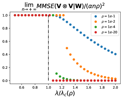
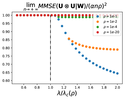
Figure 2: Sequence of MMSE curves as a function of $\lambda$ for the spiked covariance model. Left: In the sparse limit $\rho\to 0_{+}$ the suitably rescaled of the sparse signal ${\bm{V}}$ approaches a $0$–$1$ transition with a jump discontinuity at $\lambda_{c}(\rho)=\{4\gamma|\ln\rho|/(\alpha\rho)\}^{1/2}$. Right: In the asymptotic limit the MMSE for the gaussian signal ${\bm{U}}$ approaches $1$ as $\rho\to 0_{+}$. The phase transition is seen only as a higher order effect.

3  Analysis by the adaptive interpolation: the Wigner case

In this section we provide the essential architecture for the proof of theorem 1 which relies on the adaptive interpolation method [13, 14]. The proof requires concentration properties for “free energies” and “overlaps” which are deferred to appendices 6 and 7. We will also employ various known information theoretic properties of gaussian channels (I-MMSE relation, concavity of the MMSE with respect to the SNR and input distribution etc). For the convenience of the reader these are presented and adapted to our setting in appendix 11.

An essentially similar analysis can be done for theorem 2 in the Wishart case, and is deferred to appendix 5. When no confusion is possible we use the notation $\mathbb{E}\|{\bm{A}}\|^{2}=\mathbb{E}[\|{\bm{A}}\|^{2}]$.

3.1 The interpolating model.

Let $\epsilon\in[s_{n},2s_{n}]$, for a sequence tending to zero, $s_{n}=n^{-\alpha}/2\in(0,1/2)$, for $\alpha>0$ chosen later on. Let $q_{n}:[0,1]\times[s_{n},2s_{n}]\mapsto[0,\rho_{n}]$ and set

$$R_{n}(t,\epsilon)\equiv\epsilon+\lambda_{n}\int_{0}^{t}ds\,q_{n}(s,\epsilon)\,.$$

Consider the following interpolating estimation model, where $t\in[0,1]$, with accessible data $(W_{ij}(t))_{i,j}$ and $(\tilde{W}_{i}(t,\epsilon))_{i}$ obtained through

$$\begin{cases}W_{ij}(t)=W_{ji}(t)&=\sqrt{(1-t)\frac{\lambda_{n}}{n}}\,X_{i}X_{j}+Z_{ij}\,,\qquad 1\leq i<j\leq n\,,\\ \tilde{\bm{W}}(t,\epsilon)&=\sqrt{R_{n}(t,\epsilon)}\,{\bm{X}}+\tilde{\bm{Z}}\,,\end{cases}$$

with standard gaussian noise $\tilde{\bm{Z}}\sim{\cal N}(0,{\rm I}_{n})$, and $Z_{ij}=Z_{ji}\sim{\cal N}(0,1)$. The posterior associated with this model reads (here $\|-\|$ is the $\ell_{2}$ norm)

$$dP_{n,t,\epsilon}({\bm{x}}|{\bm{W}}(t),\tilde{{\bm{W}}}(t,\epsilon))=\frac{1}{\mathcal{Z}_{n,t,\epsilon}({\bm{W}}(t),\tilde{{\bm{W}}}(t,\epsilon))}\Big{(}\prod_{i=1}^{n}dP_{X,n}(x_{i})\Big{)}$$

$$\times\!\exp\!\Big{\{}\sum_{i<j}^{n}\Big{(}(1-t)\frac{\lambda_{n}}{n}\frac{x_{i}^{2}x_{j}^{2}}{2}-\sqrt{(1-t)\frac{\lambda_{n}}{n}}x_{i}x_{j}W_{ij}(t)\Big{)}+R_{n}(t,\epsilon)\frac{\|{\bm{x}}\|^{2}}{2}-\sqrt{R_{n}(t,\epsilon)}{\bm{x}}\cdot\tilde{\bm{W}}(t,\epsilon)\Big{\}}.$$

The normalization factor $\mathcal{Z}_{n,t,\epsilon}(\dots)$ is also called partition function. We also define the mutual information density for the interpolating model

$$i_{n}(t,\epsilon) \equiv\frac{1}{n}I\big{(}{\bm{X}};({\bm{W}}(t),\tilde{{\bm{W}}}(t,\epsilon))\big{)}\,.$$ (8)

The $(n,t,\epsilon,R_{n})$-dependent Gibbs-bracket (that we simply denote $\langle-\rangle_{t}$ for the sake of readability) is defined for functions $A({\bm{x}})=A$

$$\langle A({\bm{x}})\rangle_{t}=\int dP_{n,t,\epsilon}({\bm{x}}|{\bm{W}}(t),\tilde{{\bm{W}}}(t,\epsilon))\,A({\bm{x}})\,.$$ (9)

Lemma 1 (Boundary values).

The mutual information for the interpolating model verifies

$$\begin{cases}i_{n}(0,\epsilon)=\frac{1}{n}I({\bm{X}};{\bm{W}})+O(\rho_{n}s_{n})\,,\\ i_{n}(1,\epsilon)=I_{n}(X;\{\lambda_{n}\int_{0}^{1}dt\,q_{n}(t,\epsilon)\}^{1/2}X+Z)+O(\rho_{n}s_{n})\,.\end{cases}$$ (10)

where $I_{n}(X;\{\lambda_{n}\int_{0}^{1}dt\,q_{n}(t,\epsilon)\}^{1/2}X+Z)$ is the mutual information for a scalar gaussian channel with input $X\sim P_{X,n}$ and noise $Z\sim{\cal N}(0,1)$.

Proof.

We start with the chain rule for mutual information:

$$i_{n}(0,\epsilon)=\frac{1}{n}I({\bm{X}};{{\bm{W}}}(0))+\frac{1}{n}I({\bm{X}};\tilde{{\bm{W}}}(0,\epsilon)|{{\bm{W}}}(0)).$$

Note that $I({\bm{X}};{{\bm{W}}}(0))=I({\bm{X}};{\bm{W}})$ which is obvious. Moreover we claim $\frac{1}{n}I({\bm{X}};\tilde{{\bm{W}}}(0,\epsilon)|{{\bm{W}}}(0))=O(\rho_{n}s_{n})$ which yields the first identity in (10). This claim simply follows from the I-MMSE relation (appendix 11) and $R_{n}(0,\epsilon)=\epsilon$

$$\frac{d}{d\epsilon}\frac{1}{n}I({\bm{X}};\tilde{{\bm{W}}}(0,\epsilon)|{{\bm{W}}}(0))=\frac{1}{2n}{\rm MMSE}({\bm{X}}|\tilde{{\bm{W}}}(0,\epsilon),{{\bm{W}}}(0))\leq\frac{\rho_{n}}{2}\,.$$ (11)

The last inequality above is true because ${\rm MMSE}({\bm{X}}|\tilde{{\bm{W}}}(0,\epsilon),{{\bm{W}}}(0))\leq\mathbb{E}\|{\bm{X}}-\mathbb{E}\,{\bm{X}}\|^{2}=n{\rm Var}(X_{1})\leq n\rho_{n}$, as the components of ${\bm{X}}$ are i.i.d. from $P_{X,n}$. Therefore $\frac{1}{n}I({\bm{X}};\tilde{{\bm{W}}}(0,\epsilon)|{{\bm{W}}}(0))$ is $\frac{\rho_{n}}{2}$-Lipschitz in $\epsilon\in[s_{n},2s_{n}]$. Moreover we have that $I({\bm{X}};\tilde{{\bm{W}}}(0,0)|{{\bm{W}}}(0))=0$. This implies the claim.

The proof of the second identity in (10) again starts from the chain rule for mutual information

$$i_{n}(1,\epsilon)=\frac{1}{n}I({\bm{X}};\tilde{\bm{W}}(1,\epsilon))+\frac{1}{n}I({\bm{X}};{{\bm{W}}}(1)|\tilde{\bm{W}}(1,\epsilon))\,.$$

Note that $I({\bm{X}};{{\bm{W}}}(1)|\tilde{\bm{W}}(1,\epsilon))=0$ as ${{\bm{W}}}(1)$ does not depend on ${\bm{X}}$. Moreover,

$$\frac{1}{n}I({\bm{X}};\tilde{\bm{W}}(1,\epsilon))=I_{n}(X;\sqrt{R_{n}(1,\epsilon)}X+Z)=\textstyle{I_{n}(X;\{\lambda_{n}\int_{0}^{1}dt\,q_{n}(t,\epsilon)\}^{1/2}X+Z)+O(\rho_{n}s_{n})}\,.$$

because $I_{n}(X;\sqrt{\gamma}X+Z)$ is a $\frac{\rho_{n}}{2}$-Lipschitz function of $\gamma$, by an application of the I-MMSE relation (appendix 11) $\frac{d}{d\gamma}I_{n}(X;\sqrt{\gamma}X+Z)={\rm MMSE}(X|\sqrt{\gamma}X+Z)/2\leq{\rm Var}(X)/2\leq\rho_{n}/2$. ∎

3.2 Fundamental sum rule.

Proposition 1 (Sum rule).

The mutual information verifies the following sum rule:

$$\frac{1}{n}I({\bm{X}};{\bm{W}}) =i_{n}^{\rm pot}\big{(}{\textstyle\int_{0}^{1}dt\,q_{n}(t,\epsilon)};\lambda_{n},\rho_{n}\big{)}+\frac{\lambda_{n}}{4}\big{(}{\cal R}_{1}-{\cal R}_{2}-{\cal R}_{3}\big{)}+O(\rho_{n}s_{n})+O\Big{(}\frac{\lambda_{n}}{n}\Big{)}$$ (12)

with non-negative “remainders” that depend on $(n,\epsilon,R_{n})$

$$\begin{cases}{\cal R}_{1}\equiv\int_{0}^{1}dt\,\big{(}q_{n}(t,\epsilon)-\int_{0}^{1}ds\,q_{n}(s,\epsilon)\big{)}^{2}\,,\\ {\cal R}_{2}\equiv\int_{0}^{1}dt\,\mathbb{E}\big{\langle}\big{(}Q-\mathbb{E}\langle Q\rangle_{t}\big{)}^{2}\big{\rangle}_{t}\,,\\ {\cal R}_{3}\equiv\int_{0}^{1}dt\,\big{(}q_{n}(t,\epsilon)-\mathbb{E}\langle Q\rangle_{t}\big{)}^{2}\,.\end{cases}$$ (13)

where $Q=\frac{1}{n}{\bm{x}}\cdot{\bm{X}}$ is called the overlap. The constants in the $O(\cdots)$ terms are independent of $n,t,\epsilon$.

Proof.

By the fundamental theorem of calculus $i_{n}(0,\epsilon)=i_{n}(1,\epsilon)-\int_{0}^{1}dt\frac{d}{dt}i_{n}(t,\epsilon)$. Note that $i_{n}(0,\epsilon)$ and $i_{n}(1,\epsilon)$ are given by (10). The $t$-derivative of the interpolating mutual information is simply computed combining the I-MMSE relation with the chain rule for derivatives

$$\frac{d}{dt}i_{n}(t,\epsilon) =-\frac{\lambda_{n}}{2}\frac{1}{n^{2}}\sum_{i<j}\mathbb{E}\big{[}(X_{i}X_{j}-\langle x_{i}x_{j}\rangle_{t})^{2}\big{]}+\frac{\lambda_{n}q_{n}(t,\epsilon)}{2}\frac{1}{n}\mathbb{E}\|{\bm{X}}-\langle{\bm{x}}\rangle_{t}\|^{2}$$ (14)

$$=-\frac{\lambda_{n}}{4}\frac{1}{n^{2}}\mathbb{E}\|{\bm{X}}\otimes{\bm{X}}-\langle{\bm{x}}\otimes{\bm{x}}\rangle_{t}\|_{\rm F}^{2}+\frac{\lambda_{n}q_{n}(t,\epsilon)}{2}\frac{1}{n}\mathbb{E}\|{\bm{X}}-\langle{\bm{x}}\rangle_{t}\|^{2}+O\Big{(}\frac{\lambda_{n}}{n}\Big{)}\,.$$ (15)

The correction term in (15) comes from completing the diagonal terms in the sum $\sum_{i<j}$ in order to construct the matrix-MMSE, namely the first term on the r.h.s. of (15). This expression can be simplified by application of the Nishimori identities (appendix 10 contains a proof of these general identities). Starting with the second term (a vector-MMSE)

$$\frac{1}{n}\mathbb{E}\|{\bm{X}}-\langle{\bm{x}}\rangle_{t}\|^{2} =\mathbb{E}\big{[}\|{\bm{X}}\|^{2}+\|\langle{\bm{x}}\rangle_{t}\|^{2}-2{\bm{X}}\cdot\langle{\bm{x}}\rangle_{t}\big{]}$$

$$=\frac{1}{n}\mathbb{E}\big{[}\|{\bm{X}}\|^{2}-{\bm{X}}\cdot\langle{\bm{x}}\rangle_{t}\big{]}=\rho_{n}-\mathbb{E}\langle Q\rangle_{t}\,,$$ (16)

were we used $\mathbb{E}\|{\bm{X}}\|^{2}=n\rho_{n}$ and the Nishimori identity $\mathbb{E}\|\langle{\bm{x}}\rangle_{t}\|^{2}=\mathbb{E}[{\bm{X}}\cdot\langle{\bm{x}}\rangle_{t}]$. By similar manipulations we obtain for the matrix-MMSE

$$\frac{1}{n^{2}}{\rm MMSE}({\bm{X}}\otimes{\bm{X}}|\tilde{{\bm{W}}}(t,\epsilon),{{\bm{W}}}(t))=\frac{1}{n^{2}}\mathbb{E}\|{\bm{X}}\otimes{\bm{X}}-\langle{\bm{x}}\otimes{\bm{x}}\rangle_{t}\|_{\rm F}^{2}=\rho_{n}^{2}-\mathbb{E}\langle Q^{2}\rangle_{t}\,.$$ (17)

From (10), (15), (16), (17) and the fundamental theorem of calculus we deduce

$$\frac{1}{n}I({\bm{X}};{\bm{W}})= {\textstyle{I_{n}\big{(}X;\{\lambda_{n}\int_{0}^{1}dt\,q_{n}(t,\epsilon)\}^{1/2}X+Z\big{)}}}$$

$$+\frac{\lambda_{n}}{4}\int_{0}^{1}dt\,\Big{\{}\rho_{n}^{2}-\mathbb{E}\langle Q^{2}\rangle_{t}-2q_{n}(t,\epsilon)(\rho_{n}-\mathbb{E}\langle Q\rangle_{t})\Big{\}}+O(\rho_{n}s_{n})+O\Big{(}\frac{\lambda_{n}}{n}\Big{)}\,.$$

The terms on the r.h.s can be re-arranged so that the potential (3) appears, and this gives immediately the sum rule (12). ∎

Theorem 1 follows from the upper and lower bounds proven below, and applied for $s_{n}=\frac{1}{2}n^{-\alpha}$.

3.3 Upper bound: linear interpolation path.

Proposition 2 (Upper bound).

We have

$$\frac{1}{n}I({\bm{X}};{\bm{W}})\leq\inf_{q\in[0,\rho_{n}]}i_{n}^{\rm pot}(q,\lambda_{n},\rho_{n})+O(\rho_{n}s_{n})+O\Big{(}\frac{\lambda_{n}}{n}\Big{)}\,.$$

Proof.

Fix $q_{n}(t,\epsilon)=q_{n}\in[0,\rho_{n}]$ a constant independent of $\epsilon,t$. The interpolation path $R_{n}(t,\epsilon)$ is therefore a simple linear function of time. From (13) ${\cal R}_{1}$ cancels and since ${\cal R}_{2}$ and ${\cal R}_{3}$ are non-negative we get from Proposition (1)

$$\frac{1}{n}I({\bm{X}};{\bm{W}})\leq i_{n}^{\rm pot}(q,\lambda_{n},\rho_{n})+O(\rho_{n}s_{n})+O\Big{(}\frac{\lambda_{n}}{n}\Big{)}\,.$$

Note that the error terms $O(\cdots)$ are bounded independently of $q_{n}$. Therefore optimizing the r.h.s over the free parameter $q_{n}\in[0,\rho_{n}]$ yields the upper bound. ∎

3.4 Lower bound: adaptive interpolation path.

We start with a definition: the map $\epsilon\mapsto R_{n}(t,\epsilon)$ is called regular if it is a ${\cal C}^{1}$-diffeomorphism whose jacobian is greater or equal to one for all $t\in[0,1]$.

Proposition 3 (Lower bound).

Consider sequences $\lambda_{n}$ and $\rho_{n}$ satisfying $c_{1}\leq\lambda_{n}\rho_{n}\leq c_{2}n^{\gamma}$ for some constants positive constant $c_{1},c_{2}$ and $\gamma\in[0,1/2[$. Then

$$\frac{1}{n}I({\bm{X}};{\bm{W}})\geq\inf_{q\in[0,\rho_{n}]}i_{n}^{\rm pot}(q,\lambda_{n},\rho_{n})+O(\rho_{n}s_{n})+O\Big{(}\frac{\lambda_{n}}{n}\Big{)}+O\Big{(}\Big{(}\frac{\lambda_{n}^{4}\rho_{n}}{ns_{n}^{4}}\Big{)}^{1/3}\Big{)}\,.$$ (18)

Proof.

First note that the regime (2) for the sequences $\lambda_{n},\rho_{n}$ satisfies the more general condition assumed in this lemma (this is the condition in theorem 3 of appendix 4). Assume for the moment that the map $\epsilon\mapsto R_{n}(t,\epsilon)$ is regular. Then, based on Proposition 11 and identity (41) (appendix 7), we have a bound on the overlap fluctuation. Namely, for some numerical constant $C\geq 0$ independent of $n$

$$\frac{\lambda_{n}}{s_{n}}\int_{s_{n}}^{2s_{n}}d\epsilon\,{\cal R}_{2}=\frac{\lambda_{n}}{s_{n}}\int_{s_{n}}^{2s_{n}}d\epsilon\int_{0}^{1}dt\,\mathbb{E}\big{\langle}(Q-\mathbb{E}\langle Q\rangle_{n,t,R_{n}(t,\epsilon)})^{2}\big{\rangle}_{n,t,R_{n}(t,\epsilon)}\leq C\Big{(}\frac{\lambda_{n}^{4}\rho_{n}}{ns_{n}^{4}}\Big{)}^{1/3}\,.$$ (19)

Using this concentration result, and ${\cal R}_{1}\geq 0$, and averaging the sum rule (12) over $\epsilon\in[s_{n},2s_{n}]$ (recall the error terms are independent of $\epsilon$) we find

$$\frac{1}{n}I({\bm{X}};{\bm{W}})\geq \frac{1}{s_{n}}\int_{s_{n}}^{2s_{n}}d\epsilon i_{n}^{\rm pot}\big{(}{\textstyle\int_{0}^{1}dt\,q_{n}(t,\epsilon)},\lambda_{n},\rho_{n}\big{)}-\frac{\lambda_{n}}{4}\frac{1}{s_{n}}\int_{s_{n}}^{2s_{n}}d\epsilon\int_{0}^{1}dt\,\big{(}q_{n}(t,\epsilon)-\mathbb{E}\langle Q\rangle_{t}\big{)}^{2}$$

$$+O(\rho_{n}s_{n})+O\Big{(}\frac{\lambda_{n}}{n}\Big{)}+O\Big{(}\Big{(}\frac{\lambda_{n}^{4}\rho_{n}}{ns_{n}^{4}}\Big{)}^{1/3}\Big{)}\,.$$ (20)

At this stage it is natural to see if we can choose $q_{n}(t,\epsilon)$ to be the solution of $q_{n}(t,\epsilon)=\mathbb{E}\langle Q\rangle_{t}$. Setting $F_{n}(t,R_{n}(t,\epsilon))\equiv\mathbb{E}\langle Q\rangle_{n,t,R_{n}(t,\epsilon)}$, we recognize a first order ordinary differential equation

$$\frac{d}{dt}R_{n}(t,\epsilon)=F_{n}(t,R_{n}(t,\epsilon))\quad\text{with initial condition}\quad R_{n}(0,\epsilon)=\epsilon\,.$$ (21)

As $F_{n}(t,R_{n}(t,\epsilon))$ is ${\cal C}^{1}$ with bounded derivative w.r.t. its second argument the Cauchy-Lipschitz theorem implies that (21) admits a unique global solution $R_{n}^{*}(t,\epsilon)=\epsilon+\int_{0}^{t}ds\,q_{n}^{*}(s,\epsilon)$, where $q_{n}^{*}:[0,1]\times[s_{n},2s_{n}]\mapsto[0,\rho_{n}]$. Note that any solution must satisfy $q_{n}^{*}(t,\epsilon)\in[0,\rho_{n}]$ because $\mathbb{E}\langle Q\rangle_{n,t,\epsilon}\in[0,\rho_{n}]$ as can be seen from a Nishimori identity (appendix 10) and (16).

We check that $R_{n}^{*}$ is regular. By Liouville’s formula the jacobian of the flow $\epsilon\mapsto R_{n}^{*}(t,\epsilon)$ satisfies

$$\frac{d}{d\epsilon}R_{n}^{*}(t,\epsilon)=\exp\Big{\{}\int_{0}^{t}ds\,\frac{d}{dR}F_{n}(s,R)\Big{|}_{R=R_{n}^{*}(s,\epsilon)}\Big{\}}\,.$$

Applying repeatedly the Nishimori identity of Lemma 12 (appendix 10) one obtains (this computation does not present any difficulty and can be found in section 6 of [13])

$$\frac{d}{dR}F_{n}(s,R)=\frac{1}{n}\sum_{i,j=1}^{n}\mathbb{E}\big{[}(\langle x_{i}x_{j}\rangle_{n,s,R}-\langle x_{i}\rangle_{n,s,R}\langle x_{j}\rangle_{n,s,R})^{2}\big{]}\geq 0$$ (22)

so that the flow has a jacobian greater or equal to one. In particular it is locally invertible (surjective). Moreover it is injective because of the unicity of the solution of the differential equation, and therefore it is a $C^{1}$-diffeomorphism. Thus $\epsilon\mapsto R_{n}^{*}(t,\epsilon)$ is regular. With the choice $R_{n}^{*}$, i.e., by suitably adapting the interpolation path, we cancel ${\cal R}_{3}$. This yields

$$\frac{1}{n}I({\bm{X}};{\bm{W}}) \geq\frac{1}{s_{n}}\int_{s_{n}}^{2s_{n}}d\epsilon\,i_{n}^{\rm pot}\big{(}{\textstyle\int_{0}^{1}dt\,q_{n}^{*}(t,\epsilon)},\lambda_{n},\rho_{n}\big{)}+O(\cdots)$$

$$\geq\inf_{q\in[0,\rho_{n}]}i_{n}^{\rm pot}(q,\lambda_{n},\rho_{n})+O(\cdots)$$

where the $O(\cdots)$ is a shorthand notation for the three error terms in (3.4). This the desired result. ∎

Appendices

4  General results on the mutual information of sparse spiked matrix models

In this appendix we give a more general form of theorems 1 and 4 in section 2.

4.1 Spiked Wigner model

Our analysis by the adaptive interpolation method works for any regime where the sequences $\lambda_{n}$ and $\rho_{n}$ verify:

$$C\leq\lambda_{n}\rho_{n}=O(n^{\gamma})\,\quad\text{for some constants}\quad\gamma\in[0,1/2)\quad\text{and}\quad C>0\,.$$ (23)

Of course this contains the regime (2) as a special case. Our general result is a statement on the smallness of

$$\Delta I_{n}^{\rm Wig}\equiv\frac{1}{\rho_{n}|\ln\rho_{n}|}\Big{|}\frac{1}{n}I({\bm{X}};{\bm{W}})-\inf_{q\in[0,\rho_{n}]}i^{\rm pot}_{n}(q,\lambda_{n},\rho_{n})\Big{|}\,.$$

The analysis of section 3 leads to the following general theorem.

Theorem 3 (Sparse spiked Wigner model).

Let the sequences $\lambda_{n}$ and $\rho_{n}$ verify (23) and let $\alpha>0$. There exists a constant $C>0$ independent of $n$, such that the mutual information for the Wigner spike model verifies

$$\Delta I_{n}^{\rm Wig}\leq\frac{C}{|\ln\rho_{n}|}\max\Big{\{}\frac{1}{n^{\alpha}},\frac{\lambda_{n}}{n\rho_{n}},\Big{(}\frac{\lambda_{n}^{4}}{n^{1-4\alpha}\rho_{n}^{2}}\big{(}1+\lambda_{n}\rho_{n}^{2}\big{)}\Big{)}^{1/3}\Big{\}}\,.$$

In particular, choosing $\lambda_{n}=\Theta(|\ln\rho_{n}|/\rho_{n})$ (which is the appropriate scaling to observe a phase transition)

$$\Delta I_{n}^{\rm Wig}\leq C\max\Big{\{}\frac{1}{n^{\alpha}|\ln\rho_{n}|},\frac{1}{n\rho_{n}^{2}},\Big{(}\frac{|\ln\rho_{n}|}{n^{1-4\alpha}\rho_{n}^{6}}\Big{)}^{1/3}\Big{\}}\,.$$

If in addition we set $\rho_{n}=\Theta(n^{-\beta})$, $\beta\geq 0$ (which is the regime (2)) we have

$$\Delta I_{n}^{\rm Wig}\leq C\max\Big{\{}\frac{1}{n^{\alpha}\ln n},\frac{1}{n^{1-2\beta}},\Big{(}\frac{\ln n}{n^{1-4\alpha-6\beta}}\Big{)}^{1/3}\Big{\}}\,.$$

This bound vanishes as $n$ grows if $\beta\in[0,1/6)$ and $\alpha\in(0,(1-6\beta)/4]$. The last bound is optimized (up to polylog factors) setting $\alpha=(1-6\beta)/7$. In this case (again, when $\lambda_{n}=\Theta(|\ln\rho_{n}|/\rho_{n})$ and $\rho_{n}=\Theta(n^{-\beta})$)

$$\Delta I_{n}^{\rm Wig}\leq C\frac{(\ln n)^{1/3}}{n^{(1-6\beta)/7}}\,.$$

4.2 Spiked Wishart model

The following regime is of particular interest and is the one mostly studied in the literature given in the introduction on spiked covariance models:

$$\alpha_{n}\to\alpha>0\,,\quad\rho_{U,n}\to\rho_{U}>0\,,\quad\omega(1/n)=\rho_{V,n}\to 0_{+},\quad\lambda_{n}=\Theta\Big{(}\sqrt{\frac{|\ln\rho_{V,n}|}{\rho_{V,n}}}\Big{)}\,.$$ (24)

The notation $\omega(1/n)=\rho_{V,n}$ means that the sequence $\rho_{V,n}$ vanishes at a rate slower than $1/n$. The analysis of appendix 5 leads to the following general theorem on the smallness of

$$\Delta I_{n}^{\rm Wish}\equiv\frac{1}{\sqrt{\rho_{V,n}|\ln\rho_{V,n}|}}\Big{|}\frac{1}{n}I\big{(}({\bm{U}},{\bm{V}});{\bm{W}}\big{)}-\ {\adjustlimits{\inf}_{q_{U}\in[0,\rho_{U,n}]}{\sup}_{q_{V}\in[0,\rho_{V,n}]}}\,i_{n}^{\rm pot}\big{(}q_{U},q_{V},\lambda_{n},\alpha_{n},\rho_{U,n},\rho_{V,n}\big{)}\Big{|}\,.$$

Theorem 4 (Sparse spiked Wishart model).

Under the scalings (24), there exists a constant $C>0$ independent of $n$ such that the mutual information for the spiked Wishart model verifies for any $\alpha>0$

$$\Delta_{n}I^{\rm Wish}\leq C\max\Big{\{}\frac{1}{n^{\alpha}\sqrt{\rho_{V,n}|\ln\rho_{V,n}|}},\frac{|\ln\rho_{V,n}|^{-1/24}}{n^{1/3-2\alpha}\rho_{V,n}^{11/12}}\Big{(}\frac{1}{n^{\alpha}}+\sqrt{\rho_{V,n}|\ln\rho_{V,n}|}\Big{)}^{1/3}\Big{\}}\,.$$

We set $\rho_{V,n}=\Theta(n^{-\beta})$. Optimizing over $\alpha$ (up to polylog factors) such that $n^{-\alpha}<\sqrt{\rho_{V,n}|\ln\rho_{V,n}|}$ yields $\alpha=(4-3\beta)/18$. In this case the bound simplifies to

$$\Delta_{n}I^{\rm Wish}\leq C\frac{(\ln n)^{1/3}}{n^{(4-12\beta)/18}}$$

for some $C>0$. This bound vanishes if $\beta\in[0,1/3)$.

5  Proof of theorem 4 by the adaptive interpolation method

In this appendix we prove theorem 4 by the adapative interpolation method. The analysis is similar to the one of the Wigner case in section 3.

5.1 The interpolating model.

Let ${\bm{\epsilon}}=(\epsilon_{U},\epsilon_{V})\in[s_{n},2s_{n}]^{2}$ for some sequence $s_{n}=\frac{1}{2}n^{-\alpha}$. Let $q_{U,n}:[0,1]\times[s_{n},2s_{n}]\mapsto[0,\rho_{U,n}]$ and similarly for $q_{V,n}$. Set

$$\begin{cases}R_{U,n}(t,{\bm{\epsilon}})\equiv\epsilon_{U}+\lambda_{n}\int_{0}^{t}ds\,q_{U,n}(s,{\bm{\epsilon}})\,,\\ R_{V,n}(t,{\bm{\epsilon}})\equiv\epsilon_{V}+\lambda_{n}\alpha_{n}\int_{0}^{t}ds\,q_{V,n}(s,{\bm{\epsilon}})\,.\end{cases}$$

Consider the following interpolating estimation model, where $t\in[0,1]$, with accessible data

$$\begin{cases}{\bm{W}}(t)&=\sqrt{(1-t)\frac{\lambda_{n}}{n}}\,{\bm{U}}\otimes{\bm{V}}+{\bm{Z}}\,,\\ \tilde{\bm{W}}_{U}(t,{\bm{\epsilon}})&=\sqrt{R_{V,n}(t,{\bm{\epsilon}})}\,{\bm{U}}+\tilde{\bm{Z}}_{U}\,,\\ \tilde{\bm{W}}_{V}(t,{\bm{\epsilon}})&=\sqrt{R_{U,n}(t,{\bm{\epsilon}})}\,{\bm{V}}+\tilde{\bm{Z}}_{V}\,,\end{cases}$$ (25)

with independent standard gaussian noise $\tilde{\bm{Z}}_{U},\tilde{\bm{Z}}_{V}\sim{\cal N}(0,{\rm I}_{n})$, ${\bm{Z}}=(Z_{ij})_{ij}$ with i.i.d. $Z_{ij}\sim{\cal N}(0,1)$. The fact that the $R_{V,n}$ function appears as the SNR of the decoupled gaussian channel related to ${\bm{U}}$ (and vice-versa) comes from the bipartite nature of the problem. The Gibbs-bracket, simply denoted $\langle-\rangle_{t}$, is the expectation w.r.t. the posterior distribution, which is proportional to (here $\|-\|_{\rm F}$ and $\|-\|$ are the Frobenius and $\ell_{2}$ norms)

$$dP_{n,t,{\bm{\epsilon}}}\big{(}{\bm{u}},{\bm{v}}|{\bm{W}}(t),\tilde{\bm{W}}_{U}(t,{\bm{\epsilon}}),\tilde{\bm{W}}_{V}(t,{\bm{\epsilon}})\big{)}$$

$$\qquad\qquad\propto\Big{(}\prod_{i=1}^{n}dP_{U,n}(u_{i})\Big{)}\Big{(}\prod_{j=1}^{m}dP_{V,n}(v_{j})\Big{)}\exp\Big{\{}-\frac{1}{2}\big{\|}{\bm{W}}(t)-\sqrt{(1-t)\frac{\lambda_{n}}{n}}{\bm{u}}\otimes{\bm{v}}\big{\|}_{\rm F}^{2}$$

$$\qquad\qquad\qquad\qquad\qquad-\frac{1}{2}\big{\|}\tilde{\bm{W}}_{U}(t,{\bm{\epsilon}})-\sqrt{R_{V,n}(t,{\bm{\epsilon}})}\,{\bm{u}}\big{\|}^{2}-\frac{1}{2}\big{\|}\tilde{\bm{W}}_{V}(t,{\bm{\epsilon}})-\sqrt{R_{U,n}(t,{\bm{\epsilon}})}\,{\bm{v}}\big{\|}^{2}\Big{\}}\,.$$

The mutual information density for this interpolating model is

$$i_{n}(t,{\bm{\epsilon}})\equiv\frac{1}{n}I\big{(}({\bm{U}},{\bm{V}});({\bm{W}}(t),\tilde{{\bm{W}}}_{U}(t,{\bm{\epsilon}}),\tilde{{\bm{W}}}_{V}(t,{\bm{\epsilon}}))\big{)}\,.$$

The proof of the following lemma is similar to the one of Lemma 1.

Lemma 2 (Boundary values).

Let $\bar{\rho}_{n}=\max(\rho_{U,n},\rho_{V,n})$, $U\sim P_{U,n}$, $V\sim P_{V,n}$ and $Z\sim{\cal N}(0,1)$. Then

$$\begin{cases}i_{n}(0,{\bm{\epsilon}})=\frac{1}{n}I(({\bm{U}},{\bm{V}});{\bm{W}})+O(\bar{\rho}_{n}s_{n})\,,\\ i_{n}(1,{\bm{\epsilon}})=I_{n}(U;\{\lambda_{n}\alpha_{n}\int_{0}^{1}q_{V,n}(s,{\bm{\epsilon}})\}^{1/2}U\!+\!Z)\!+\!\alpha_{n}I_{n}(V;\{\lambda_{n}\int_{0}^{1}q_{U,n}(s,{\bm{\epsilon}})\}^{1/2}V\!+\!Z)\!+\!O(\bar{\rho}_{n}s_{n})\,.\end{cases}$$

5.2 Fundamental sum-rule.

As before, our proof is bases on an important sum-rule.

Proposition 4 (Sum rule).

Let $\bar{\rho}_{n}=\max(\rho_{U,n},\rho_{V,n})$, $\alpha_{n}=m/n$, $U\sim P_{U,n}$, $V\sim P_{V,n}$ and $Z\sim{\cal N}(0,1)$. Then

$$\frac{1}{n}I(({\bm{U}},{\bm{V}});{\bm{W}})=I_{n}(U;\{\lambda_{n}\alpha_{n}\textstyle{\int_{0}^{1}q_{V,n}}(s,{\bm{\epsilon}})\}^{1/2}U+Z)+\alpha_{n}I_{n}(V;\{\lambda_{n}\textstyle{\int_{0}^{1}q_{U,n}}(s,{\bm{\epsilon}})\}^{1/2}V+Z)$$

$$\qquad+\frac{\lambda_{n}\alpha_{n}}{2}\rho_{U,n}\rho_{V,n}+\frac{\lambda_{n}\alpha_{n}}{2}\int_{0}^{1}dt\Big{\{}\mathbb{E}\langle Q_{U}\rangle_{t}\mathbb{E}\langle Q_{V}\rangle_{t}-\mathbb{E}\langle Q_{U}Q_{V}\rangle_{t}\Big{\}}+O(\bar{\rho}_{n}s_{n})$$

$$\qquad+\frac{\lambda_{n}\alpha_{n}}{2}\int_{0}^{1}dt\Big{\{}q_{V,n}(t,{\bm{\epsilon}})(\mathbb{E}\langle Q_{U}\rangle_{t}-\rho_{U,n})+q_{U,n}(t,{\bm{\epsilon}})(\mathbb{E}\langle Q_{V}\rangle_{t}-\rho_{V,n})-\mathbb{E}\langle Q_{U}\rangle_{t}\mathbb{E}\langle Q_{V}\rangle_{t}\Big{\}}$$

where the overlaps are defined as

$$Q_{U}\equiv\frac{1}{n}{\bm{u}}\cdot{\bm{U}}\,,\qquad Q_{V}\equiv\frac{1}{m}{\bm{v}}\cdot{\bm{V}}\,.$$

Proof.

We compare the boundaries values (10) using the fundamental theorem of calculus $i_{n}(0,{\bm{\epsilon}})=i_{n}(1,{\bm{\epsilon}})-\int_{0}^{1}dt\frac{d}{dt}i_{n}(t,{\bm{\epsilon}})$. Using the I-MMSE formula (first equality) and then the Nishimori identity (second equality) we have

$$\frac{d}{dt}i_{n}(t,{\bm{\epsilon}})$$

$$=-\frac{\lambda_{n}\alpha_{n}}{2nm}\mathbb{E}\|{\bm{U}}\otimes{\bm{V}}-\langle{\bm{u}}\otimes{\bm{v}}\rangle_{t}\|_{\rm F}^{2}\!+\!\frac{\lambda_{n}\alpha_{n}q_{V,n}(t,{\bm{\epsilon}})}{2n}\mathbb{E}\|{\bm{U}}-\langle{\bm{u}}\rangle_{t}\|^{2}\!+\!\frac{\lambda_{n}\alpha_{n}q_{U,n}(t,{\bm{\epsilon}})}{2m}\mathbb{E}\|{\bm{V}}-\langle{\bm{v}}\rangle_{t}\|^{2}$$

$$\overset{\rm N}{=}\frac{\lambda_{n}\alpha_{n}}{2}\Big{\{}\mathbb{E}\langle Q_{U}Q_{V}\rangle_{t}-\rho_{U,n}\rho_{V,n}+q_{V,n}(t,{\bm{\epsilon}})(\rho_{U,n}-\mathbb{E}\langle Q_{U}\rangle_{t})+q_{U,n}(t,{\bm{\epsilon}})(\rho_{V,n}-\mathbb{E}\langle Q_{V}\rangle_{t})\Big{\}}\,.$$

The $\rm N$ stands for “Nishimori”, and each time we use the Nishimori identity of Lemma 12 for a simplification we write a $\rm N$ on top of the equality. Replacing this result and the boundary values (10) in the fundamental theorem of calculus yields the sum rule after few lines of algebra. ∎

We now derive two matching bounds, under the scalings (24), which implie Theorem 4.

5.3 Upper bound: partially adaptive interpolation path.

We start again with the simplest bound:

Proposition 5 (Upper bound).

Under the scalings (24) we have

$$\frac{1}{n}I(({\bm{U}},{\bm{V}});{\bm{W}}) \leq{\adjustlimits{\inf}_{q_{U}\in[0,\rho_{U,n}]}{\sup}_{q_{V}\in[0,\rho_{V,n}]}}\,i_{n}^{\rm pot}\big{(}q_{U},q_{V},\lambda_{n},\alpha_{n},\rho_{U,n},\rho_{V,n}\big{)}$$

$$\qquad\qquad\qquad+O\Big{(}s_{n}+\frac{|\ln\rho_{V,n}|^{11/24}}{s_{n}^{2}n^{1/3}\rho_{V,n}^{9/24}}\Big{(}s_{n}+\sqrt{\rho_{V,n}|\ln\rho_{V,n}|}\Big{)}^{1/3}\Big{)}\,.$$ (26)

Proof.

For this bound only one of the interpolation function is adapted. Consider the following Cauchy problem for $R_{n}(t,{\bm{\epsilon}})=(R_{U,n}(t,{\bm{\epsilon}}),R_{V,n}(t,{\bm{\epsilon}}))$:

$$\frac{dR_{n}}{dt}(t,{\bm{\epsilon}})=\big{(}\lambda_{n}q_{U},G_{V,n}(t,R_{n}(t,{\bm{\epsilon}}))\big{)},\qquad R_{n}(0,{\bm{\epsilon}})={\bm{\epsilon}}\,,$$

where $q_{U}\in[0,\rho_{U,n}]$ and $G_{V,n}(t,R_{n}(t,{\bm{\epsilon}}))\equiv\lambda_{n}\alpha_{n}\mathbb{E}\langle Q_{V}\rangle_{t}\in[0,\lambda_{n}\alpha_{n}\rho_{V,n}]$, i.e.,

$$\big{(}q_{U,n}(t,{\bm{\epsilon}}),q_{V,n}(t,{\bm{\epsilon}})\big{)}=\big{(}q_{U},\mathbb{E}\langle Q_{V}\rangle_{t}\big{)},\qquad R_{n}(0,{\bm{\epsilon}})={\bm{\epsilon}}\,.$$

By the Cauchy-Lipschitz theorem this ODE admits a unique global solution

$$\textstyle R_{n}^{*}(t,{\bm{\epsilon}})=(R_{U,n}^{*}(t,{\bm{\epsilon}})=\epsilon_{U}+\lambda_{n}q_{U,n}t,R_{V,n}^{*}(t,{\bm{\epsilon}})=\epsilon_{V}+\lambda_{n}\alpha_{n}\int_{0}^{t}ds\,q^{*}_{V,n}(s,{\bm{\epsilon}}))\,.$$

Because the function $(q_{U},\mathbb{E}\langle Q_{V}\rangle_{t})$ is ${\cal C}^{1}$ the solution $R_{n}^{*}$ is ${\cal C}^{1}$ in all its arguments. By the Liouville formula the Jacobian determinant $J_{n}(t,{\bm{\epsilon}})$ of the flow ${\bm{\epsilon}}\mapsto R_{n}^{*}(t,{\bm{\epsilon}})$ satisfies

$$J_{n}(t,{\bm{\epsilon}})\equiv{\rm det}\Big{(}\frac{\partial R_{n,t}(t,{\bm{\epsilon}})}{\partial{\bm{\epsilon}}}\Big{)}=\exp\Big{\{}\int_{0}^{t}\frac{\partial G_{V,n}}{\partial R_{V}}(s,R_{U,n}^{*}(s,{\bm{\epsilon}}),R_{V}=R_{V,n}^{*}(s,{\bm{\epsilon}}))ds\Big{\}}\geq 1\,.$$ (27)

We show at the end of the proof that $\frac{\partial G_{V,n}}{\partial R_{V}}\geq 0$. The intuition is the same as before: increasing the SNR $R_{V}$ cannot decrease the overlap $\mathbb{E}\langle Q_{V}\rangle_{t}$, or equivalently it cannot increase the MMSE $\rho_{V,n}-\mathbb{E}\langle Q_{V}\rangle_{t}$. The flow ${\bm{\epsilon}}\mapsto R_{n}^{*}(t,{\bm{\epsilon}})$ thus has Jacobian greater or equal to one, and is surjective. It is also injective by unicity of the solution of the differential equation, and is thus a ${\cal C}^{1}$-diffeomorphism. A $\mathcal{C}^{1}$-diffeomrophic flow with Jacobian greater or equal to one is called regular.

By the Cauchy-Schwarz inequality and Fubini’s theorem we have

$$\frac{\lambda_{n}\alpha_{n}}{2s_{n}^{2}}\Big{|}\int d{\bm{\epsilon}}\int_{0}^{1}dt\Big{\{}\mathbb{E}\langle Q_{U}\rangle_{t}\mathbb{E}\langle Q_{V}\rangle_{t}-\mathbb{E}\langle Q_{U}Q_{V}\rangle_{t}\Big{\}}\Big{|}$$

$$\qquad=\frac{\lambda_{n}\alpha_{n}}{2s_{n}^{2}}\Big{|}\int_{0}^{1}dt\int d{\bm{\epsilon}}\,\mathbb{E}\big{\langle}(Q_{U}-\mathbb{E}\langle Q_{U}\rangle_{t})(Q_{V}-\mathbb{E}\langle Q_{V}\rangle_{t})\big{\rangle}_{t}\Big{|}$$

$$\qquad\qquad\leq\frac{\lambda_{n}\alpha_{n}}{2s_{n}^{2}}\int_{0}^{1}dt\Big{\{}\int d{\bm{\epsilon}}\,\mathbb{E}\big{\langle}(Q_{U}-\mathbb{E}\langle Q_{U}\rangle_{t})^{2}\big{\rangle}_{t}\Big{\}}^{1/2}\Big{\{}\int d{\bm{\epsilon}}\,\mathbb{E}\big{\langle}(Q_{V}-\mathbb{E}\langle Q_{V}\rangle_{t})^{2}\big{\rangle}_{t}\Big{\}}^{1/2}\,.$$

By the regularity of the flow we are allowed to use Propositions 12, 13 of section 7. Together with inequality (55) and a similar one for ${\cal L}_{U}$ (see section 7) we obtain under the scalings (24),

$$\frac{\lambda_{n}\alpha_{n}}{2s_{n}^{2}}\Big{|}\int d{\bm{\epsilon}}\int_{0}^{1}dt\Big{\{}\mathbb{E}\langle Q_{U}\rangle_{t}\mathbb{E}\langle Q_{V}\rangle_{t}-\mathbb{E}\langle Q_{U}Q_{V}\rangle_{t}\Big{\}}\Big{|}$$

$$\qquad\qquad\leq\frac{C}{s_{n}^{2}}\sqrt{\frac{|\ln\rho_{V,n}|}{\rho_{V,n}}}\Big{(}\frac{1}{n}\sqrt{\frac{|\ln\rho_{V,n}|}{\rho_{V,n}}}\big{(}s_{n}+\sqrt{\rho_{V,n}|\ln\rho_{V,n}|}\big{)}^{2}\times\frac{(\ln\rho_{V,n})^{2}}{n\rho_{V,n}}\Big{)}^{1/6}$$

$$\qquad\qquad=C\frac{|\ln\rho_{V,n}|^{11/24}}{s_{n}^{2}n^{1/3}\rho_{V,n}^{9/24}}\Big{(}s_{n}+\sqrt{\rho_{V,n}|\ln\rho_{V,n}|}\Big{)}^{1/3}\,.$$ (28)

Therefore, averaging the sum-rule over ${\bm{\epsilon}}\in[s_{n},2s_{n}]^{2}$ and using the solution $R^{*}_{n}$ of the above Cauchy problem, we obtain

$$\frac{1}{n}I(({\bm{U}},{\bm{V}});{\bm{W}}) =\frac{1}{s_{n}^{2}}\int_{[s_{n},2s_{n}]^{2}}d{\bm{\epsilon}}\,i_{n}^{\rm pot}\big{(}q_{U},{\textstyle\int_{0}^{1}}q_{V,n}^{*}(t,{\bm{\epsilon}})dt,\lambda_{n},\alpha_{n},\rho_{U,n},\rho_{V,n}\big{)}$$

$$\qquad\qquad\qquad+O\Big{(}s_{n}+\frac{|\ln\rho_{V,n}|^{11/24}}{s_{n}^{2}n^{1/3}\rho_{V,n}^{9/24}}\Big{(}s_{n}+\sqrt{\rho_{V,n}|\ln\rho_{V,n}|}\Big{)}^{1/3}\Big{)}\,.$$

Because this inequality is true for any $q_{U}\in[0,\rho_{U,n}]$ we obtain the result.

It remains to prove that $\frac{\partial G_{V,n}}{\partial R_{V}}\geq 0$, i.e., $\frac{\partial\mathbb{E}\langle Q_{V}\rangle_{t}}{\partial R_{V}}\geq 0$. We drop un-necessary dependencies. Let $\Delta\geq 0$. Consider the following modification of the model (25):

$$\begin{cases}{\bm{W}}&=\sqrt{(1-t)\frac{\lambda_{n}}{n}}\,{\bm{U}}\otimes{\bm{V}}+{\bm{Z}}\,,\\ \hat{\bm{W}}_{U}(R_{V},\Delta)&={\bm{U}}+\tilde{\bm{Z}}_{U}/\sqrt{R_{V}}+\hat{\bm{Z}}_{U}\sqrt{\Delta/R_{V}}\,,\\ \tilde{\bm{W}}_{V}&=\sqrt{R_{U}}\,{\bm{V}}+\tilde{\bm{Z}}_{V}\,,\end{cases}$$

where $\hat{\bm{Z}}_{U}\sim{\cal N}(0,{\rm I}_{n})$ independently of the rest. By stability of the gaussian distribution under addition we have in law $\tilde{\bm{Z}}_{U}/\sqrt{R_{V}}+\hat{\bm{Z}}_{U}\sqrt{\Delta/R_{V}}=\tilde{\bm{Z}}_{U}\sqrt{(\Delta+1)/R_{V}}$, therefore the MMSE for model (25) ${\rm MMSE}({\bm{V}}|{\bm{W}},\tilde{\bm{W}}_{U}(R_{V}),\tilde{\bm{W}}_{V})$ (we made explicit the dependence of $\tilde{\bm{W}}_{U}$ in $R_{V}=R_{V,n}(t,{\bm{\epsilon}})$) verifies

$${\rm MMSE}({\bm{V}}|{\bm{W}},\hat{\bm{W}}_{U}(R_{V},\Delta),\tilde{\bm{W}}_{V})={\rm MMSE}({\bm{V}}|{\bm{W}},\tilde{\bm{W}}_{U}(R_{V}/(\Delta+1)),\tilde{\bm{W}}_{V})\,.$$

We then have

$${\rm MMSE}({\bm{V}}|{\bm{W}},\tilde{\bm{W}}_{U}(R_{V}),\tilde{\bm{W}}_{V})={\rm MMSE}({\bm{V}}|{\bm{W}},\hat{\bm{W}}_{U}(R_{V},\Delta),\tilde{\bm{W}}_{V},\hat{\bm{Z}}_{U})$$

$$\qquad\qquad\leq{\rm MMSE}({\bm{V}}|{\bm{W}},\hat{\bm{W}}_{U}(R_{V},\Delta),\tilde{\bm{W}}_{V})={\rm MMSE}({\bm{V}}|{\bm{W}},\tilde{\bm{W}}_{U}(R_{V}/(\Delta+1)),\tilde{\bm{W}}_{V})$$

where the inequality follows from Lemma 16. Because $\frac{R_{V}}{\Delta+1}\leq R_{V}$, ${\rm MMSE}({\bm{V}}|{\bm{W}},\tilde{\bm{W}}_{U}(R_{V}),\tilde{\bm{W}}_{V})$ is non-increasing in $R_{V}$. Recalling

$${\rm MMSE}({\bm{V}}|{\bm{W}},\tilde{\bm{W}}_{U}(R_{V}),\tilde{\bm{W}}_{V})\overset{\rm N}{=}\rho_{V,n}-\mathbb{E}\langle Q_{V}\rangle_{t}$$

this proves $\frac{\partial G_{V,n}}{\partial R_{V}}\geq 0$.

We provide here an alternative proof. Consider the interpolating model (25) where a positive quantity $\Delta$ is added to $R_{V}$. We denote $I_{\Delta}\big{(}({\bm{U}},{\bm{V}});({\bm{W}},\tilde{{\bm{W}}}_{U},\tilde{{\bm{W}}}_{V})\big{)}$ the mutual information for this new model, so $i_{n}(t,{\bm{\epsilon}})=\frac{1}{n}I_{0}\big{(}({\bm{U}},{\bm{V}});({\bm{W}},\tilde{{\bm{W}}}_{U},\tilde{{\bm{W}}}_{V})\big{)}$. By Lemma 17 this model is mutual information-wise equivalent to the following one:

$$\begin{cases}{\bm{W}}&=\sqrt{(1-t)\frac{\lambda_{n}}{n}}\,{\bm{U}}\otimes{\bm{V}}+{\bm{Z}}\,,\\ \tilde{\bm{W}}_{U}&=\sqrt{R_{V}}\,{\bm{U}}+\tilde{\bm{Z}}_{U}\,,\\ \hat{\bm{W}}_{U}(\Delta)&=\sqrt{\Delta}\,{\bm{U}}+\hat{\bm{Z}}_{U}\,,\\ \tilde{\bm{W}}_{V}(t,{\bm{\epsilon}})&=\sqrt{R_{U}}\,{\bm{V}}+\tilde{\bm{Z}}_{V}\,,\end{cases}$$ (29)

where $\hat{\bm{Z}}_{U}\sim{\cal N}(0,{\rm I}_{n})$ independently of the rest. Namely,

$$I_{\Delta}\big{(}({\bm{U}},{\bm{V}});({\bm{W}},\tilde{{\bm{W}}}_{U},\tilde{{\bm{W}}}_{V})\big{)}=I\big{(}({\bm{U}},{\bm{V}});({\bm{W}},\tilde{{\bm{W}}}_{U},\hat{{\bm{W}}}_{U}(\Delta),\tilde{{\bm{W}}}_{V})\big{)}\,.$$

Using the chain rule for mutual information it is re expressed as

$$I_{\Delta}\big{(}{\bm{V}};({\bm{W}}(t),\tilde{{\bm{W}}}_{U}(t,{\bm{\epsilon}}),\tilde{{\bm{W}}}_{V}(t,{\bm{\epsilon}}))\big{)}+I_{\Delta}\big{(}{\bm{U}};({\bm{W}}(t),\tilde{{\bm{W}}}_{U})|{\bm{V}}\big{)}$$

$$\qquad=I\big{(}{\bm{V}};({\bm{W}},\tilde{{\bm{W}}}_{U},\hat{{\bm{W}}}_{U}(\Delta),\tilde{{\bm{W}}}_{V})\big{)}+I\big{(}{\bm{U}};({\bm{W}},\tilde{{\bm{W}}}_{U},\hat{{\bm{W}}}_{U}(\Delta))|{\bm{V}}\big{)}\,.$$

The two mutual information conditioned of ${\bm{V}}$ are independent of $R_{V}$. Taking a $R_{V}$ derivative on both sides, by the I-MMSE formula Lemma 13 the associated MMSE’s verify

$${\rm MMSE}_{\Delta}({\bm{V}}|{\bm{W}},\tilde{{\bm{W}}}_{U},\tilde{{\bm{W}}}_{V})={\rm MMSE}({\bm{V}}|{\bm{W}},\tilde{{\bm{W}}}_{U},\hat{{\bm{W}}}_{U}(\Delta),\tilde{{\bm{W}}}_{V})\,.$$

Lemma 16 then implies

$${\rm MMSE}_{\Delta}({\bm{V}}|{\bm{W}},\tilde{{\bm{W}}}_{U},\tilde{{\bm{W}}}_{V})\leq{\rm MMSE}({\bm{V}}|{\bm{W}},\tilde{{\bm{W}}}_{U},\tilde{{\bm{W}}}_{V})$$

or equivalently

$$\mathbb{E}\langle Q_{V}\rangle_{t,\Delta}\geq\mathbb{E}\langle Q_{V}\rangle_{t}$$

where ${\rm MMSE}_{\Delta}({\bm{V}}|\cdots)$ and $\mathbb{E}\langle Q_{V}\rangle_{t,\Delta}$ are the average MMSE and overlap for ${\bm{V}}$ corresponding to model (29) or equivalently model (25) with $R_{V,n}$ replaced by $R_{V,n}+\Delta$. This proves $\frac{\partial G_{V,n}}{\partial R_{V}}\geq 0$. ∎

5.4 Lower bound: fully adaptive interpolation path.

For the converse bound we need to adapt both interpolating functions.

Proposition 6 (Lower bound).

Under the scalings (24) the converse of the bound (26) holds.

Proof.

Consider this time the following Cauchy problem:

$$\frac{dR_{n}}{dt}(t,{\bm{\epsilon}})=\big{(}G_{U,n}(t,R_{n}(t,{\bm{\epsilon}})),G_{V,n}(t,R_{n}(t,{\bm{\epsilon}}))\big{)},\qquad R_{n}(0,{\bm{\epsilon}})={\bm{\epsilon}}\,,$$ (30)

with the functions $G_{U,n}(t,R_{n}(t,{\bm{\epsilon}}))\equiv\lambda_{n}(\rho_{U,n}-{\rm MMSE}(U|\sqrt{\lambda_{n}\alpha_{n}\mathbb{E}\langle Q_{V}\rangle_{t}}U+Z))\in[0,\lambda_{n}\rho_{U,n}]$ and $G_{V,n}(t,R_{n}(t,{\bm{\epsilon}}))\equiv\lambda_{n}\alpha_{n}\mathbb{E}\langle Q_{V}\rangle_{t}\in[0,\lambda_{n}\alpha_{n}\rho_{V,n}]$, or in other words,

$$\big{(}q_{U,n}(t,{\bm{\epsilon}}),q_{V,n}(t,{\bm{\epsilon}})\big{)}=\big{(}\rho_{U,n}-{\rm MMSE}(U|\sqrt{\lambda_{n}\alpha_{n}\mathbb{E}\langle Q_{V}\rangle_{t}}U+Z),\mathbb{E}\langle Q_{V}\rangle_{t}\big{)},\qquad R_{n}(0,{\bm{\epsilon}})={\bm{\epsilon}}\,.$$

This ODE admits a unique global ${\cal C}^{1}$ solution $R_{n}^{*}(t,{\bm{\epsilon}})=(R_{U,n}^{*}(t,{\bm{\epsilon}}),R_{V,n}^{*}(t,{\bm{\epsilon}}))$ by the Cauchy-Lipschitz theorem. By the Liouville formula, the Jacobian determinant of the flow ${\bm{\epsilon}}\mapsto R_{n}^{*}(t,{\bm{\epsilon}})$ satisfies

$$J_{n}(t,{\bm{\epsilon}}) =\exp\Big{\{}\int_{0}^{t}\Big{(}\frac{\partial G_{U,n}}{\partial R_{U}}(s,R_{U}=R_{U,n}^{*}(s,{\bm{\epsilon}}),R_{V,n}^{*}(s,{\bm{\epsilon}}))$$

$$\qquad\qquad\qquad\qquad+\frac{\partial G_{V,n}}{\partial R_{V}}(s,R_{U,n}^{*}(s,{\bm{\epsilon}}),R_{V}=R_{V,n}^{*}(s,{\bm{\epsilon}}))\Big{)}ds\Big{\}}\,.$$

Both partial derivatives are positive by the same proof as in the previous paragraph. Then using teh same arguments as previously we conclude that the flow is regular (a $\mathcal{C}^{1}$-diffeomorphism with Jacobian greater or equal to one). Using this solution we can thus use Propositions 12, 13 of section 7 to deduce from the sum rule of Proposition 4

$$\frac{1}{n}I(({\bm{U}},{\bm{V}});{\bm{W}})$$

$$\quad=\frac{1}{s_{n}^{2}}\int d{\bm{\epsilon}}\Big{[}I_{n}(U;\{\lambda_{n}\alpha_{n}\textstyle{\int_{0}^{1}q^{*}_{V,n}}(t,{\bm{\epsilon}})dt\}^{1/2}U+Z)+\alpha_{n}I_{n}(V;\{\lambda_{n}\textstyle{\int_{0}^{1}q^{*}_{U,n}}(t,{\bm{\epsilon}})dt\}^{1/2}V+Z)$$

$$\qquad\qquad+\frac{\lambda_{n}\alpha_{n}}{2}\int_{0}^{1}dt(q^{*}_{U,n}(t,{\bm{\epsilon}})-\rho_{U,n})(q^{*}_{V,n}(t,{\bm{\epsilon}})-\rho_{V,n})\Big{]}$$

$$\qquad\qquad\qquad\qquad+O\Big{(}s_{n}+\frac{|\ln\rho_{V,n}|^{11/24}}{s_{n}^{2}n^{1/3}\rho_{V,n}^{9/24}}\big{(}s_{n}+\sqrt{\rho_{V,n}|\ln\rho_{V,n}|}\big{)}^{1/3}\Big{)}$$

$$\quad\geq\frac{1}{s_{n}^{2}}\int d{\bm{\epsilon}}\int_{0}^{1}dt\,i_{n}^{\rm pot}\big{(}q_{U,n}^{*}(t,{\bm{\epsilon}}),q_{V,n}^{*}(t,{\bm{\epsilon}}),\lambda_{n},\alpha_{n},\rho_{U,n},\rho_{V,n}\big{)}+O(\cdots)\,.$$

To get the last inequality we used the concavity in the SNR of the mutual information for gaussian channels, see Lemma 14 of section 11. Now note that

$$i_{n}^{\rm pot}\big{(}q_{U,n}^{*}(t,{\bm{\epsilon}}),q_{V,n}^{*}(t,{\bm{\epsilon}}),\lambda_{n},\alpha_{n},\rho_{U,n},\rho_{V,n}\big{)}=\sup_{q_{V}\in[0,\rho_{V,n}]}i_{n}^{\rm pot}\big{(}q_{U,n}^{*}(t,{\bm{\epsilon}}),q_{V},\lambda_{n},\alpha_{n},\rho_{U,n},\rho_{V,n}\big{)}\,.$$

Indeed, the function $g_{n}(q_{U},\cdot):q_{V}\mapsto i_{n}^{\rm pot}(q_{U},q_{V};\lambda_{n},\alpha_{n},\rho_{U,n},\rho_{V,n})$ is concave (by concavity of the mutual information in the SNR, see Lemma 14) with $q_{V}$-derivative

$$\frac{dg}{dq_{V}}(q_{U},q_{V})=\frac{\lambda_{n}\alpha_{n}}{2}\big{(}q_{u}-\rho_{U,n}+{\rm MMSE}(U|\sqrt{\lambda_{n}\alpha_{n}q_{V}}U+Z)\big{)}$$

(using the I-MMSE relation). By definition of the solution $R_{n}^{*}$ of the ODE (30) we have

$$\frac{dg}{dq_{V}}(q_{U,n}^{*}(t,{\bm{\epsilon}}),q_{V}=q_{V,n}^{*}(t,{\bm{\epsilon}}))=0\,.$$

By concavity this corresponds to a maximum. Therefore

$$\frac{1}{n}I(({\bm{U}},{\bm{V}});{\bm{W}}) \geq\frac{1}{s_{n}^{2}}\int d{\bm{\epsilon}}\int_{0}^{1}dt\,\sup_{q_{V}\in[0,\rho_{V,n}]}i_{n}^{\rm pot}\big{(}q_{U,n}^{*}(t,{\bm{\epsilon}}),q_{V},\lambda_{n},\alpha_{n},\rho_{U,n},\rho_{V,n}\big{)}+O(\cdots)$$

$$\geq{\adjustlimits{\inf}_{q_{U}\in[0,\rho_{U,n}]}{\sup}_{q_{V}\in[0,\rho_{V,n}]}}\,i_{n}^{\rm pot}\big{(}q_{U},q_{V},\lambda_{n},\alpha_{n},\rho_{U,n},\rho_{V,n}\big{)}+O(\cdots)\,.$$

∎

6  Concentration of free energies

For this appendix it is convenient to use the language of statistical mechanics.

6.1 Statistical mechanics notations for the spiked Wigner (interpolating) model.

We express the posterior of the interpolating model

$$dP_{n,t,\epsilon}({\bm{x}}|{\bm{W}}(t),\tilde{{\bm{W}}}(t,\epsilon))=\frac{1}{\mathcal{Z}_{n,t,\epsilon}({\bm{W}}(t),\tilde{{\bm{W}}}(t,\epsilon))}$$

$$\qquad\qquad\qquad\qquad\qquad\qquad\times\Big{(}\prod_{i=1}^{n}dP_{X,n}(x_{i})\Big{)}\exp\big{\{}-{\cal H}_{n,t,\epsilon}({\bm{x}},{\bm{W}}(t),\tilde{{\bm{W}}}(t,\epsilon))\big{\}}$$ (31)

with normalization constant (partition function) $\mathcal{Z}_{n,t,\epsilon}$ and “hamiltonian”

$${\cal H}_{n,t,\epsilon}({\bm{x}},{\bm{W}}(t),\tilde{{\bm{W}}}(t,\epsilon))={\cal H}_{n,t,\epsilon}({\bm{x}},{\bm{X}},{\bm{Z}},\tilde{\bm{Z}})$$ (32)

$$\ \equiv\sum_{i<j}^{n}\Big{(}(1-t)\frac{\lambda_{n}}{n}\frac{x_{i}^{2}x_{j}^{2}}{2}-\sqrt{(1-t)\frac{\lambda_{n}}{n}}x_{i}x_{j}W_{ij}(t)\Big{)}+R_{n}(t,\epsilon)\frac{\|{\bm{x}}\|^{2}}{2}-\sqrt{R_{n}(t,\epsilon)}{\bm{x}}\cdot\tilde{\bm{W}}(t,\epsilon)$$

$$\ =(1-t)\lambda_{n}\sum_{i<j}^{n}\Big{(}\frac{x_{i}^{2}x_{j}^{2}}{2n}-\frac{x_{i}x_{j}X_{i}X_{j}}{n}-\frac{x_{i}x_{j}Z_{ij}}{\sqrt{n(1-t)\lambda_{n}}}\Big{)}+R_{n}(t,\epsilon)\Big{(}\frac{\|{\bm{x}}\|^{2}}{2}-{\bm{x}}\cdot{\bm{X}}-\frac{{\bm{x}}\cdot\tilde{{\bm{Z}}}}{\sqrt{R_{n}(t,\epsilon)}}\Big{)}.$$

It will also be convenient to work with “free energies” rather than mutual informations. The free energy $F_{n}(t,\epsilon)$ and (its expectation $f_{n}(t,\epsilon)$) for the interpolating model is simply minus the (expected) log-partition function:

$$F_{n,t,\epsilon}({\bm{W}}(t),\tilde{{\bm{W}}}(t,\epsilon)) \equiv-\frac{1}{n}\ln\mathcal{Z}_{n,t,\epsilon}({\bm{W}}(t),\tilde{{\bm{W}}}(t,\epsilon))\,,$$ (33)

$$f_{n}(t,\epsilon) \equiv\mathbb{E}\,F_{n,t,\epsilon}({\bm{W}}(t),\tilde{{\bm{W}}}(t,\epsilon))\,.$$ (34)

The expectation $\mathbb{E}$ carries over the data. The averaged free energy is related to the mutual information $i_{n}(t,\epsilon)$ given by (8) through

$$i_{n}(t,\epsilon)=f_{n}(t,\epsilon)+\frac{n-1}{n}\frac{\rho^{2}\lambda(1-t)}{4}+\frac{\rho R_{n}(t,\epsilon)}{2}\,.$$ (35)

6.2 Statistical mechanics notations for the spiked Wishart (interpolating) model.

Let the set ${\cal D}_{n,t,{\bm{\epsilon}}}=\{{\bm{W}}(t),\tilde{\bm{W}}_{U}(t,{\bm{\epsilon}}),\tilde{\bm{W}}_{V}(t,{\bm{\epsilon}})\}$. In the Wishart case the posterior reads

$$dP_{n,t,\epsilon}({\bm{u}},{\bm{v}}|{\cal D}_{n,t,{\bm{\epsilon}}}) =\frac{1}{{\cal Z}_{n,t,\epsilon}({\cal D}_{n,t,{\bm{\epsilon}}})}\Big{(}\prod_{i=1}^{n}dP_{U,n}(u_{i})\Big{)}\Big{(}\prod_{j=1}^{m}dP_{V,n}(v_{j})\Big{)}$$

$$\qquad\qquad\times\exp\big{\{}-{\cal H}_{n,t,\bm{\epsilon}}({\bm{u}},{\bm{v}},{\cal D}_{n,t,{\bm{\epsilon}}})\big{\}}$$ (36)

with hamiltonian

$${\cal H}_{n,t,\bm{\epsilon}}({\bm{u}},{\bm{v}},{\cal D}_{n,t,{\bm{\epsilon}}}) \equiv(1-t)\frac{\lambda_{n}}{n}\frac{\|{\bm{u}}\|^{2}\|{\bm{v}}\|^{2}}{2}-\sqrt{(1-t)\frac{\lambda_{n}}{n}}{\bm{u}}\cdot({\bm{W}}(t){\bm{v}})$$

$$\quad+R_{V,n}(t,{\bm{\epsilon}})\frac{\|{\bm{u}}\|^{2}}{2}-\sqrt{R_{V,n}(t,{\bm{\epsilon}})}{\bm{u}}\cdot\tilde{\bm{W}}_{U}(t,{\bm{\epsilon}})$$

$$\quad+R_{U,n}(t,{\bm{\epsilon}})\frac{\|{\bm{v}}\|^{2}}{2}-\sqrt{R_{U,n}(t,{\bm{\epsilon}})}{\bm{v}}\cdot\tilde{\bm{W}}_{V}(t,{\bm{\epsilon}})$$

$$=(1-t)\frac{\lambda_{n}}{n}\frac{\|{\bm{u}}\|^{2}\|{\bm{v}}\|^{2}}{2}-(1-t)\frac{\lambda_{n}}{n}({\bm{u}}\cdot{\bm{U}})({\bm{v}}\cdot{\bm{V}})-\sqrt{(1-t)\frac{\lambda_{n}}{n}}{\bm{u}}\cdot({\bm{Z}}{\bm{v}})$$

$$\quad+R_{V,n}(t,{\bm{\epsilon}})\frac{\|{\bm{u}}\|^{2}}{2}-{R_{V,n}(t,{\bm{\epsilon}})}{\bm{u}}\cdot{\bm{U}}-\sqrt{R_{V,n}(t,{\bm{\epsilon}})}{\bm{u}}\cdot\tilde{\bm{Z}}_{U}$$

$$\quad+R_{U,n}(t,{\bm{\epsilon}})\frac{\|{\bm{v}}\|^{2}}{2}-{R_{U,n}(t,{\bm{\epsilon}})}{\bm{v}}\cdot{\bm{V}}-\sqrt{R_{U,n}(t,{\bm{\epsilon}})}{\bm{v}}\cdot\tilde{\bm{Z}}_{V}\,.$$ (37)

The free energy and its expectation (over the data) are

$$F_{n,t,\bm{\epsilon}}({\cal D}_{n,t,{\bm{\epsilon}}}) \equiv-\frac{1}{n}\ln\mathcal{Z}_{n,t,\epsilon}({\cal D}_{n,t,{\bm{\epsilon}}})\,,$$ (38)

$$f_{n}(t,\bm{\epsilon}) \equiv\mathbb{E}\,F_{n,t,\bm{\epsilon}}({\cal D}_{n,t,{\bm{\epsilon}}})\,.$$ (39)

Similarly to (35) the averaged free energy is related to the mutual information by an additive constant (linear in $R_{U,n}$ and $R_{V,n}$) that does not change its concavity properties.

6.3 Free energy concentration for the Wigner case

In this section we prove a concentration identity for the free energy (33) onto its average (34).

Proposition 7 (Free energy concentration for the spiked Wigner model).

We have

$$\mathbb{E}\Big{[}\Big{(}F_{n,t,\epsilon}({\bm{W}}(t), \tilde{{\bm{W}}}(t,\epsilon))-f_{n}(t,\epsilon)\Big{)}^{2}\Big{]}\leq\frac{2\rho_{n}S^{2}}{n}\Big{(}(2s_{n}+\lambda_{n}\rho_{n})^{2}+S^{4}\Big{)}+\frac{3}{2}\frac{\lambda_{n}\rho_{n}^{2}}{n}+2\frac{s_{n}\rho_{n}}{n}\,.$$

Considering sequences $\lambda_{n}$ and $\rho_{n}$ verifying (23) and with $s_{n}=(1/2)n^{-\alpha}\to 0_{+}$ the bound simplifies to $C(S)\lambda_{n}^{2}\rho_{n}^{3}/n$ with positive constant $C(S)\leq\frac{5}{2}+8S^{2}+2S^{6}$.

The proof is based on two classical concentration inequalities,

Proposition 8 (Gaussian Poincaré inequality).

Let ${\bm{U}}=(U_{1},\dots,U_{N})$ be a vector of $N$ independent standard normal random variables. Let $g:\mathbb{R}^{N}\to\mathbb{R}$ be a continuously differentiable function. Then

$${{\rm Var}}(g({\bm{U}}))\leq\mathbb{E}\|\nabla g({\bm{U}})\|^{2}\,.$$

Proposition 9 (Efron-Stein inequality).

Let $\,\mathcal{U}\subset\mathbb{R}$, and a function $g:\mathcal{U}^{N}\to\mathbb{R}$. Let $\,{\bm{U}}=(U_{1},\dots,U_{N})$ be a vector of $N$ independent random variables with law $P_{U}$ that take values in $\,\mathcal{U}$. Let $\,{\bm{U}}^{(i)}$ a vector which differs from ${\bm{U}}$ only by its $i$-th component, which is replaced by $U_{i}^{\prime}$ drawn from $P_{U}$ independently of $\,{\bm{U}}$. Then

$${{\rm Var}}(g({\bm{U}}))\leq\frac{1}{2}\sum_{i=1}^{N}\mathbb{E}_{{\bm{U}}}\mathbb{E}_{U_{i}^{\prime}}\big{[}(g({\bm{U}})-g({\bm{U}}^{(i)}))^{2}\big{]}\,.$$

We start by proving the concentration w.r.t. the gaussian variables. It is convenient to make explicit the dependence of the partition function of the interpolating model in the independent quenched variables instead of the data: ${\cal Z}_{n,t,\epsilon}({\bm{X}},{\bm{Z}},\tilde{\bm{Z}})=\mathcal{Z}_{n,t,\epsilon}({\bm{W}}(t),\tilde{{\bm{W}}}(t,\epsilon))$.

Lemma 3 (Concentration w.r.t. the gaussian variables).

We have

$$\mathbb{E}\Big{[}\Big{(}\frac{1}{n}\ln{\cal Z}_{n,t,\epsilon}({\bm{X}},{\bm{Z}},\tilde{\bm{Z}})-\frac{1}{n}\mathbb{E}_{{\bm{Z}},\tilde{\bm{Z}}}\ln{\cal Z}_{n,t,\epsilon}({\bm{X}},{\bm{Z}},\tilde{\bm{Z}})\Big{)}^{2}\Big{]}\leq\frac{3}{2}\frac{\lambda_{n}\rho_{n}^{2}}{n}+2\frac{s_{n}\rho_{n}}{n}\,.$$

Proof.

Fix all variables except ${\bm{Z}},\tilde{\bm{Z}}$. Let $g({\bm{Z}},\tilde{\bm{Z}})\equiv-\frac{1}{n}\ln{\cal Z}_{n,t,\epsilon}({\bm{X}},{\bm{Z}},\tilde{\bm{Z}})$ be the free energy seen as a function of the gaussian variables only. The free energy gradient reads $\mathbb{E}\|\nabla g\|^{2}=\mathbb{E}\|\nabla_{\bm{Z}}g\|^{2}+\mathbb{E}\|\nabla_{\tilde{\bm{Z}}}g\|^{2}$. Let us denote ${\cal H}(t)\equiv{\cal H}_{n,t,\epsilon}$ the interpolating Hamiltonian (32).

$$\mathbb{E}\|\nabla_{\bm{Z}}g\|^{2}=\frac{1}{n^{2}}\mathbb{E}\|\langle\nabla_{\bm{Z}}{\cal H}(t)\rangle_{t}\|^{2} =\frac{(1-t)\lambda_{n}}{n^{3}}\sum_{i<j}\mathbb{E}[\langle x_{i}x_{j}\rangle_{t}^{2}]\leq\frac{(1-t)\lambda_{n}}{n^{3}}\sum_{i<j}\mathbb{E}\langle(x_{i}x_{j})^{2}\rangle_{t}$$

$$\overset{\rm N}{=}\frac{(1-t)\lambda_{n}}{n^{3}}\sum_{i<j}\mathbb{E}[(X_{i}X_{j})^{2}]\leq\frac{\lambda_{n}\rho_{n}^{2}}{2n}\,.$$

where we used a Nishimori identity for the last equality. Similarly, and using $\lambda_{n}\rho_{n}\geq 1$ and $s_{n}<1/2$,

$$\mathbb{E}\|\nabla_{\tilde{\bm{Z}}}g\|^{2}=\frac{R(\epsilon)}{n^{2}}\mathbb{E}\|\langle{\bm{x}}\rangle_{t}\|^{2}\leq\frac{R(\epsilon)}{n^{2}}\mathbb{E}\langle\|{\bm{x}}\|^{2}\rangle_{t}\overset{\rm N}{=}\frac{R(\epsilon)}{n^{2}}\mathbb{E}\|{\bm{X}}\|^{2}\leq\frac{(2s_{n}+\rho_{n}\lambda_{n})\rho_{n}}{n}\,.$$

Therefore Proposition 8 directly implies the stated result. ∎

We now consider the fluctuations due to the signal realization:

Lemma 4 (Concentration w.r.t. the spike).

We have

$$\mathbb{E}\Big{[}\Big{(}-\frac{1}{n}\mathbb{E}_{{\bm{Z}},\tilde{\bm{Z}}}\ln{\cal Z}_{n,t,\epsilon}({\bm{X}},{\bm{Z}},\tilde{\bm{Z}})-f_{n}(t,\epsilon)\Big{)}^{2}\Big{]}\leq\frac{2\rho_{n}S^{2}}{n}\Big{(}(2s_{n}+\lambda_{n}\rho_{n})^{2}+S^{4}\Big{)}\,.$$

Proof.

Let $g({\bm{X}})\equiv-\frac{1}{n}\mathbb{E}_{{\bm{Z}},\tilde{\bm{Z}}}\ln{\cal Z}_{n,t,\epsilon}({\bm{X}},{\bm{Z}},\tilde{\bm{Z}})$. Define ${\bm{X}}^{(i)}$ as a vector with same entries as ${\bm{X}}$ except the $i$-th one that is replaced by $X_{i}^{\prime}$ drawn independently from $P_{X,n}$. Let us estimate $(g({\bm{X}})-g({\bm{X}}^{(i)}))^{2}$ by interpolation. Let ${\cal H}(t,s{\bm{X}}+(1-s){\bm{X}}^{(i)})$ be the interpolating Hamiltonian (32) with ${\bm{X}}$ replaced by $s{\bm{X}}+(1-s){\bm{X}}^{(i)}$. Then

$$\mathbb{E}\big{[}(g({\bm{X}})- g({\bm{X}}^{(i)}))^{2}\big{]}=\mathbb{E}\Big{[}\Big{(}\int_{0}^{1}ds\frac{dg}{ds}(s{\bm{X}}+(1-s){\bm{X}}^{(i)})\Big{)}^{2}\Big{]}$$

$$=\frac{1}{n^{2}}\mathbb{E}\Big{[}\Big{(}\int_{0}^{1}ds\Big{\langle}\frac{d{\cal H}}{ds}(t,s{\bm{X}}+(1-s){\bm{X}}^{(i)})\Big{\rangle}_{t}\Big{)}^{2}\Big{]}$$

$$=\frac{1}{n^{2}}\mathbb{E}\Big{[}\Big{(}(X_{i}-X_{i}^{\prime})\Big{\langle}R_{\epsilon}(t)x_{i}+\frac{1-t}{n}x_{i}\sum_{j(\neq i)}X_{j}x_{j}\Big{\rangle}_{t}\Big{)}^{2}\Big{]}$$

$$\leq\frac{2}{n^{2}}\mathbb{E}\Big{[}(X_{i}-X_{i}^{\prime})^{2}\Big{(}\langle x_{i}\rangle_{t}^{2}(2s_{n}+\lambda_{n}\rho_{n})^{2}+\frac{1}{n^{2}}\sum_{j,k(\neq i)}X_{j}X_{k}\langle x_{i}x_{j}\rangle_{t}\langle x_{i}x_{k}\rangle_{t}\Big{)}\Big{]}$$

$$\leq\frac{2}{n^{2}}\mathbb{E}\big{[}(X_{i}-X_{i}^{\prime})^{2}\big{]}\Big{(}S^{2}(2s_{n}+\lambda_{n}\rho_{n})^{2}+S^{6}\Big{)}$$

$$\leq\frac{4\rho_{n}S^{2}}{n^{2}}\Big{(}(2s_{n}+\lambda_{n}\rho_{n})^{2}+S^{4}\Big{)}\,.$$

We used $(a+b)^{2}\leq 2(a^{2}+b^{2})$ for the second inequality and $\mathbb{E}[(X_{i}-X_{i}^{\prime})^{2}]=2{\rm Var}(X_{i})\leq 2\rho_{n}$. Therefore Proposition 9 implies the claim. ∎

6.4 Free energy concentration for the Wishart case

In this section we prove a concentration identity for the free energy (38) onto its average (39).

Proposition 10 (Free energy concentration for the spiked Wishart model).

We have

$$\mathbb{E}\Big{[}\Big{(}F_{n,t,\bm{\epsilon}}({\bm{W}}(t),\tilde{\bm{W}}_{U}(t,{\bm{\epsilon}}),\tilde{\bm{W}}_{V}(t,{\bm{\epsilon}}))-f_{n}(t,\bm{\epsilon})\Big{)}^{2}\Big{]}\!\leq\!\frac{C_{F,n}}{n}$$

where

$$C_{F,n} \equiv 2\rho_{U,n}S^{2}\big{\{}(2s_{n}+\lambda_{n}\alpha_{n}\rho_{V,n})^{2}+\alpha_{n}^{2}S^{4}\big{\}}+2\alpha_{n}\rho_{V,n}S^{2}\big{\{}(2s_{n}+\lambda_{n}\rho_{U,n})^{2}+S^{4}\big{\}}$$

$$\hskip 142.26378pt+3\lambda_{n}\alpha_{n}\rho_{U,n}\rho_{V,n}+2s_{n}(1+\alpha_{n})\bar{\rho}_{n}\,.$$

In the particular case of the scalings (24) we have $C_{F,n}\leq C|\ln\rho_{V,n}|$ for some positive constant $C$ that may depend on anything but $n$.

The proofs are brief as they are similar to those for the spiked Wigner model. The partition function expressed with the independent quenched variables is ${\cal Z}_{n,t,\bm{\epsilon}}({\bm{U}},{\bm{V}},{\bm{Z}},\tilde{\bm{Z}}_{U},\tilde{\bm{Z}}_{V})\equiv{\cal Z}_{n,t,\bm{\epsilon}}({\cal D}_{n,t,{\bm{\epsilon}}})$.

Lemma 5 (Concentration w.r.t. the gaussian variables).

Let $\bar{\rho}_{n}\equiv\max(\rho_{U,n},\rho_{V,n})$. We have

$$\mathbb{E}\Big{[}\Big{(}\frac{1}{n}\ln{\cal Z}_{n,t,\bm{\epsilon}}({\bm{U}},{\bm{V}},{\bm{Z}},\tilde{\bm{Z}}_{U},\tilde{\bm{Z}}_{V})-\frac{1}{n}\mathbb{E}_{{\bm{Z}},\tilde{\bm{Z}}_{U},\tilde{\bm{Z}}_{V}}\ln{\cal Z}_{n,t,\bm{\epsilon}}({\bm{U}},{\bm{V}},{\bm{Z}},\tilde{\bm{Z}}_{U},\tilde{\bm{Z}}_{V})\Big{)}^{2}\Big{]}$$

$$\qquad\qquad\qquad\qquad\qquad\qquad\qquad\qquad\qquad\qquad\leq 3\frac{\lambda_{n}\alpha_{n}\rho_{U,n}\rho_{V,n}}{n}+2\frac{s_{n}(1+\alpha_{n})\bar{\rho}_{n}}{n}\,.$$

Proof.

Let $g({\bm{Z}},\tilde{\bm{Z}}_{U},\tilde{\bm{Z}}_{V})$ be the free energy (38) seen as a function of only the gaussian variables. Based on the hamiltonian expression (37) we compute the gradient:

$$\mathbb{E}\|\nabla_{\bm{Z}}g\|^{2}=\frac{(1-t)\lambda_{n}}{n^{3}}\mathbb{E}\|\langle{\bm{u}}\otimes{\bm{v}}\rangle_{t}\|_{\rm F}^{2}\leq\frac{\lambda_{n}}{n^{3}}\mathbb{E}\|{\bm{U}}\|^{2}\mathbb{E}\|{\bm{V}}\|^{2}\leq\frac{\lambda_{n}\alpha_{n}\rho_{U,n}\rho_{V,n}}{n}$$

where the bracket is w.r.t. the interpolating model posterior (36). We used that ${\bm{u}},{\bm{U}}\in\mathbb{R}^{n}$ while ${\bm{v}},{\bm{V}}\in\mathbb{R}^{m}$, and $\alpha_{n}\equiv m/n$. Similarly

$$\mathbb{E}\|\nabla_{\tilde{\bm{Z}}_{U}}g\|^{2} =\frac{R_{V,n}(t,{\bm{\epsilon}})^{2}}{n^{2}}\mathbb{E}\|\langle{\bm{u}}\rangle_{t}\|^{2}\leq\frac{(2s_{n}+\rho_{V,n}\alpha_{n}\lambda_{n})\rho_{U,n}}{n}\,,$$

$$\mathbb{E}\|\nabla_{\tilde{\bm{Z}}_{V}}g\|^{2} =\frac{R_{U,n}(t,{\bm{\epsilon}})^{2}}{n^{2}}\mathbb{E}\|\langle{\bm{v}}\rangle_{t}\|^{2}\leq\frac{(2s_{n}+\rho_{U,n}\lambda_{n})\alpha_{n}\rho_{V,n}}{n}\,.$$

Proposition 8 implies the result. ∎

Lemma 6 (Concentration w.r.t. the spikes).

We have

$$\mathbb{E}\Big{[}\Big{(}-\frac{1}{n}\mathbb{E}_{{\bm{Z}},\tilde{\bm{Z}}_{U},\tilde{\bm{Z}}_{V}}\ln{\cal Z}_{n,t,\bm{\epsilon}}({\bm{U}},{\bm{V}},{\bm{Z}},\tilde{\bm{Z}}_{U},\tilde{\bm{Z}}_{V})-f_{n}(t,\bm{\epsilon})\Big{)}^{2}\Big{]}$$

$$\hskip 56.9055pt\leq\frac{2\rho_{U,n}S^{2}}{n}\Big{(}(2s_{n}+\lambda_{n}\alpha_{n}\rho_{V,n})^{2}+\alpha_{n}^{2}S^{4}\Big{)}+\frac{2\alpha_{n}\rho_{V,n}S^{2}}{n}\Big{(}(2s_{n}+\lambda_{n}\rho_{U,n})^{2}+S^{4}\Big{)}\,.$$

Proof.

Let $g({\bm{U}})$ be the free energy (38) seen as a function of ${\bm{U}}$ only. Define ${\bm{U}}^{(i)}$ as a vector with same entries as ${\bm{U}}$ except the $i$-th one that is replaced by $U_{i}^{\prime}$ drawn independently from $P_{U,n}$. Let ${\cal H}(t,s{\bm{U}}+(1-s){\bm{U}}^{(i)})$ be the interpolating Hamiltonian (37) with ${\bm{U}}$ replaced by $s{\bm{U}}+(1-s){\bm{U}}^{(i)}$. We bound

$$\mathbb{E}\big{[}(g({\bm{U}})-g({\bm{U}}^{(i)}))^{2}\big{]} =\frac{1}{n^{2}}\mathbb{E}\Big{[}\Big{(}\int_{0}^{1}ds\Big{\langle}\frac{d{\cal H}}{ds}(t,s{\bm{U}}+(1-s){\bm{U}}^{(i)})\Big{\rangle}_{t}\Big{)}^{2}\Big{]}$$

$$=\frac{1}{n^{2}}\mathbb{E}\Big{[}\Big{(}(U_{i}-U_{i}^{\prime})\Big{\langle}R_{V,n}u_{i}+\frac{1-t}{n}u_{i}({\bm{v}}\cdot{\bm{V}})\Big{\rangle}_{t}\Big{)}^{2}\Big{]}$$

$$\leq\frac{2}{n^{2}}\mathbb{E}\Big{[}(U_{i}-U_{i}^{\prime})^{2}\Big{(}\langle u_{i}\rangle_{t}^{2}(2s_{n}+\lambda_{n}\alpha_{n}\rho_{V,n})^{2}+\frac{1}{n^{2}}\langle u_{i}({\bm{v}}\cdot{\bm{V}})\rangle_{t}^{2}\Big{)}\Big{]}$$

$$\leq\frac{2}{n^{2}}\mathbb{E}\big{[}(U_{i}-U_{i}^{\prime})^{2}\big{]}\Big{(}S^{2}(2s_{n}+\lambda_{n}\alpha_{n}\rho_{V,n})^{2}+\alpha_{n}^{2}S^{6}\Big{)}$$

$$\leq\frac{4\rho_{U,n}S^{2}}{n^{2}}\Big{(}(2s_{n}+\lambda_{n}\alpha_{n}\rho_{V,n})^{2}+\alpha_{n}^{2}S^{4}\Big{)}\,.$$

Similarly, and with an anlogous notation ${\bm{V}}^{(i)}$, we obtain

$$\mathbb{E}\big{[}(g({\bm{V}})-g({\bm{V}}^{(i)}))^{2}\big{]}\leq\frac{4\rho_{V,n}S^{2}}{n^{2}}\Big{(}(2s_{n}+\lambda_{n}\rho_{U,n})^{2}+S^{4}\Big{)}\,.$$

Proposition 9 then implies the claim. ∎

7  Concentration for the overlaps

7.1 Overlap concentration for the Wigner case: proof of inequality (19)

The derivations below will apply for any $t\in[0,1]$ so we drop all un-necessary notations and indices. Only the dependence of the free energies in $R(\epsilon)\equiv R_{n}(t,\epsilon)$ matters, so we denote $F(R(\epsilon))\equiv F_{n,t,\epsilon}({\bm{W}}(t),\tilde{{\bm{W}}}(t,\epsilon))$ and $f(R(\epsilon))\equiv f_{n}(t,\epsilon)$.

Let $\mathcal{L}$ be the $R(\epsilon)$-derivative of the Hamiltonian (32) divided by $n$:

$$\mathcal{L}({\bm{x}},{\bm{X}},\tilde{\bm{Z}})=\mathcal{L}\equiv\frac{1}{n}\frac{d{\cal H}_{n,t,\epsilon}}{dR(\epsilon)}=\frac{1}{n}\Big{(}\frac{\|{\bm{x}}\|^{2}}{2}-{\bm{x}}\cdot{\bm{X}}-\frac{{\bm{x}}\cdot\tilde{\bm{Z}}}{2\sqrt{R(\epsilon)}}\Big{)}\,.$$ (40)

The overlap fluctuations are upper bounded by those of $\mathcal{L}$, which are easier to control, as

$$\mathbb{E}\big{\langle}(Q-\mathbb{E}\langle Q\rangle_{t})^{2}\big{\rangle}_{t}\leq 4\,\mathbb{E}\big{\langle}(\mathcal{L}-\mathbb{E}\langle\mathcal{L}\rangle_{t})^{2}\big{\rangle}_{t}\,.$$ (41)

The bracket is again the expectation w.r.t. the posterior of the interpolating model (9). A detailed derivation of this inequality can be found in appendix 8 and involves only elementary algebra using the Nishimori identity and integrations by parts w.r.t. the gaussian noise $\tilde{\bm{Z}}$.

We have the following identities: for any given realisation of the quenched disorder

$$\frac{dF}{dR(\epsilon)} =\langle\mathcal{L}\rangle_{t}\,,$$ (42)

$$\frac{1}{n}\frac{d^{2}F}{dR(\epsilon)^{2}} =-\big{\langle}(\mathcal{L}-\langle\mathcal{L}\rangle_{t})^{2}\big{\rangle}_{t}+\frac{1}{4n^{2}R(\epsilon)^{3/2}}\langle{\bm{x}}\rangle_{t}\cdot\tilde{\bm{Z}}\,.$$ (43)

The gaussian integration by part formula (75) with hamiltonian (32) yields

$$\frac{\mathbb{E}\big{\langle}\tilde{\bm{Z}}\cdot{\bm{x}}\big{\rangle}_{t}}{\sqrt{R(\epsilon)}}=\mathbb{E}\big{\langle}\|{\bm{x}}\|^{2}\big{\rangle}_{t}-\mathbb{E}\|\langle{\bm{x}}\rangle_{t}\|^{2}\overset{\rm N}{=}\mathbb{E}\big{\langle}\|{\bm{x}}\|^{2}\big{\rangle}_{t}-\mathbb{E}\big{\langle}{\bm{X}}\cdot{\bm{x}}\big{\rangle}_{t}=\mathbb{E}\big{\langle}\|{\bm{x}}\|^{2}\big{\rangle}_{t}-n\,\mathbb{E}\langle Q\rangle_{t}\,.$$ (44)

Therefore averaging (42) and (43) we find

$$\frac{df}{dR(\epsilon)} =\mathbb{E}\langle\mathcal{L}\rangle_{t}\overset{\rm N}{=}-\frac{1}{2}\mathbb{E}\langle Q\rangle_{t}\,,$$ (45)

$$\frac{1}{n}\frac{d^{2}f}{dR(\epsilon)^{2}} =-\mathbb{E}\big{\langle}(\mathcal{L}-\langle\mathcal{L}\rangle_{t})^{2}\big{\rangle}_{t}+\frac{1}{4n^{2}R(\epsilon)}\mathbb{E}\big{\langle}\|{\bm{x}}-\langle{\bm{x}}\rangle_{t}\|^{2}\big{\rangle}_{t}\,.$$ (46)

We always work under the assumption that the map $\epsilon\in[s_{n},2s_{n}]\mapsto R(\epsilon)\in[R(s_{n}),R(2s_{n})]$ is regular, and do not repeat this assumption in the statements below. The concentration inequality (19) is a direct consequence of the following result (combined with Fubini’s theorem):

Proposition 11 (Total fluctuations of ${\cal L}$).

Let the sequences $\lambda_{n}$ and $\rho_{n}$ verify (23). Then

$$\int_{s_{n}}^{2s_{n}}d\epsilon\,\mathbb{E}\big{\langle}(\mathcal{L}-\mathbb{E}\langle\mathcal{L}\rangle_{t})^{2}\big{\rangle}_{t}\leq C\Big{(}\frac{\lambda_{n}\rho_{n}}{ns_{n}}\big{(}1+\lambda_{n}\rho_{n}^{2}\big{)}\Big{)}^{1/3}$$

for a constant $C>0$ that is independent of $n$, as long as the r.h.s. is $\omega(1/n)$.

The proof of this proposition is broken in two parts, using the decomposition

$$\mathbb{E}\big{\langle}(\mathcal{L}-\mathbb{E}\langle\mathcal{L}\rangle_{t})^{2}\big{\rangle}_{t} =\mathbb{E}\big{\langle}(\mathcal{L}-\langle\mathcal{L}\rangle_{t})^{2}\big{\rangle}_{t}+\mathbb{E}\big{[}(\langle\mathcal{L}\rangle_{t}-\mathbb{E}\langle\mathcal{L}\rangle_{t})^{2}\big{]}\,.$$

Thus it suffices to prove the two following lemmas. The first lemma expresses concentration w.r.t. the posterior distribution (or “thermal fluctuations”) and is a direct consequence of concavity properties of the average free energy and the Nishimori identity.

Lemma 7 (Thermal fluctuations of $\cal L$).

We have

$$\int_{s_{n}}^{2s_{n}}d\epsilon\,\mathbb{E}\big{\langle}(\mathcal{L}-\langle\mathcal{L}\rangle_{t})^{2}\big{\rangle}_{t}\leq\frac{\rho_{n}}{n}\Big{(}1+\frac{\ln 2}{4}\Big{)}\,.$$

Proof.

We emphasize again that the interpolating free energy (8) is here viewed as a function of $R(\epsilon)$. In the argument that follows we consider derivatives of this function w.r.t. $R(\epsilon)$. By (46)

$$\mathbb{E}\big{\langle}(\mathcal{L}-\langle\mathcal{L}\rangle_{t})^{2}\big{\rangle}_{t} =-\frac{1}{n}\frac{d^{2}f}{dR(\epsilon)^{2}}+\frac{1}{4n^{2}R(\epsilon)}\big{(}\mathbb{E}\big{\langle}\|{\bm{x}}\|^{2}\big{\rangle}_{t}-\mathbb{E}\|\langle{\bm{x}}\rangle_{t}\|^{2}\big{)}$$

$$\leq-\frac{1}{n}\frac{d^{2}f}{dR(\epsilon)^{2}}+\frac{\rho_{n}}{4n\epsilon}\,,$$ (47)

where we used $R(\epsilon)\geq\epsilon$ and $\frac{1}{n}\mathbb{E}\langle\|{\bm{x}}\|^{2}\rangle_{t}\overset{\rm N}{=}\mathbb{E}[X_{1}^{2}]=\rho_{n}$. We integrate this inequality over $\epsilon\in[s_{n},2s_{n}]$. Recall the map $\epsilon\mapsto R(\epsilon)$ has a Jacobian $\geq 1$, is ${\cal C}^{1}$ and has a well defined ${\cal C}^{1}$ inverse since we have assumed that it is regular. Thus integrating (47) and performing a change of variable (to get the second inequality) we obtain

$$\int_{s_{n}}^{2s_{n}}d\epsilon\,\mathbb{E}\big{\langle}(\mathcal{L}-\langle\mathcal{L}\rangle_{t})^{2}\big{\rangle}_{t} \leq-\frac{1}{n}\int_{s_{n}}^{2s_{n}}d\epsilon\,\frac{d^{2}f}{dR(\epsilon)^{2}}+\frac{\rho_{n}}{4n}\int_{s_{n}}^{2s_{n}}\,\frac{d\epsilon}{\epsilon}$$

$$\leq-\frac{1}{n}\int_{R(s_{n})}^{R(2s_{n})}dR(\epsilon)\,\frac{d^{2}f}{dR(\epsilon)^{2}}+\frac{\rho_{n}}{4n}\int_{s_{n}}^{2s_{n}}\,\frac{d\epsilon}{\epsilon}$$

$$=\frac{1}{n}\Big{(}\frac{df}{dR(\epsilon)}(R(s_{n}))-\frac{df}{dR(\epsilon)}(R(2s_{n}))\Big{)}+\frac{\rho_{n}}{4n}\ln 2\,.$$

We have $|f^{\prime}(R(\epsilon))|=|\mathbb{E}\langle Q\rangle_{t}/2|\leq\rho_{n}/2$ so the first term is certainly smaller in absolute value than $\rho_{n}/n$. This concludes the proof of Lemma 7. ∎

The second lemma expresses the concentration w.r.t. the quenched disorder variables and is a consequence of the concentration of the free energy onto its average (w.r.t. the quenched variables).

Lemma 8 (Quenched fluctuations of $\cal L$).

Let the sequences $\lambda_{n}$ and $\rho_{n}$ verify (23). Then

$$\int_{s_{n}}^{2s_{n}}d\epsilon\,\mathbb{E}\big{[}(\langle\mathcal{L}\rangle_{t}-\mathbb{E}\langle\mathcal{L}\rangle_{t})^{2}\big{]}\leq C\Big{(}\frac{\lambda_{n}\rho_{n}}{ns_{n}}\big{(}1+\lambda_{n}\rho_{n}^{2}\big{)}\Big{)}^{1/3}$$

for a constant $C>0$ that is independent of $n$, as long as the r.h.s. is $\omega(1/n)$.

Proof.

Consider the following functions of $R(\epsilon)$:

$$\tilde{F}(R(\epsilon))\equiv F(R(\epsilon))+S\frac{\sqrt{R(\epsilon)}}{n}\sum_{i=1}^{n}|\tilde{Z}_{i}|\,,$$

$$\tilde{f}(R(\epsilon))\equiv\mathbb{E}\,\tilde{F}(R(\epsilon))=f(R(\epsilon))+S\sqrt{R(\epsilon)}\mathbb{E}\,|\tilde{Z}_{1}|\,.$$ (48)

Because of (43) we see that the second derivative of $\tilde{F}(R(\epsilon))$ w.r.t. $R(\epsilon)$ is negative so that it is concave. Note $F(R(\epsilon))$ itself is not necessarily concave in $R(\epsilon)$, although $f(R(\epsilon))$ is. Concavity of $f(R(\epsilon))$ is not obvious from (46) (obtained from differentiating $\mathbb{E}\langle{\cal L}\rangle_{t}$ w.r.t. $R(\epsilon)$) but can be seen from (77) (obtained instead by differentiating $-\frac{1}{2}\mathbb{E}\langle{Q}\rangle_{t}$) which reads $\frac{d}{dR(\epsilon)}\mathbb{E}\langle Q\rangle_{t}=-2\frac{d^{2}}{dR(\epsilon)^{2}}f\geq 0$. Equivalently it follows from the relation (35) between mutual information and free energy and the concavity of the mutual information Lemma 14. Evidently $\tilde{f}(R(\epsilon))$ is concave too. Concavity then allows to use the following standard lemma:

Lemma 9 (A bound for concave functions).

Let $G(x)$ and $g(x)$ be concave functions. Let $\delta>0$ and define $C^{-}_{\delta}(x)\equiv g^{\prime}(x-\delta)-g^{\prime}(x)\geq 0$ and $C^{+}_{\delta}(x)\equiv g^{\prime}(x)-g^{\prime}(x+\delta)\geq 0$. Then

$$|G^{\prime}(x)-g^{\prime}(x)|\leq\delta^{-1}\sum_{u\in\{x-\delta,\,x,\,x+\delta\}}|G(u)-g(u)|+C^{+}_{\delta}(x)+C^{-}_{\delta}(x)\,.$$

First, from (7.1) we have

$$\tilde{F}(R(\epsilon))-\tilde{f}(R(\epsilon))=F(R(\epsilon))-f(R(\epsilon))+S\sqrt{R(\epsilon)}A_{n}$$ (49)

with $A_{n}\equiv\frac{1}{n}\sum_{i=1}^{n}|\tilde{Z}_{i}|-\mathbb{E}\,|\tilde{Z}_{1}|$. Second, from (42), (45) we obtain for the $R(\epsilon)$-derivatives

$$\tilde{F}^{\prime}(R(\epsilon))-\tilde{f}^{\prime}(R(\epsilon))=\langle\mathcal{L}\rangle_{t}-\mathbb{E}\langle\mathcal{L}\rangle_{t}+\frac{SA_{n}}{2\sqrt{R(\epsilon)}}\,.$$ (50)

From (49) and (50) it is then easy to show that Lemma 9 implies

$$|\langle\mathcal{L}\rangle_{t}-\mathbb{E}\langle\mathcal{L}\rangle_{t}| \leq\delta^{-1}\sum_{u\in\{R(\epsilon)-\delta,\,R(\epsilon),\,R(\epsilon)+\delta\}}\big{(}|F(u)-f(u)|+S|A_{n}|\sqrt{u}\big{)}$$

$$\qquad\qquad\qquad\qquad+C_{\delta}^{+}(R(\epsilon))+C_{\delta}^{-}(R(\epsilon))+\frac{S|A_{n}|}{2\sqrt{\epsilon}}$$ (51)

where $C_{\delta}^{-}(R(\epsilon))\equiv\tilde{f}^{\prime}(R(\epsilon)-\delta)-\tilde{f}^{\prime}(R(\epsilon))\geq 0$ and $C_{\delta}^{+}(R(\epsilon))\equiv\tilde{f}^{\prime}(R(\epsilon))-\tilde{f}^{\prime}(R(\epsilon)+\delta)\geq 0$. We used $R(\epsilon)\geq\epsilon$ for the term $S|A_{n}|/(2\sqrt{\epsilon})$. Note that $\delta$ will be chosen later on strictly smaller than $s_{n}$ so that $R(\epsilon)-\delta\geq\epsilon-\delta\geq s_{n}-\delta$ remains positive. Remark that by independence of the noise variables $\mathbb{E}[A_{n}^{2}]=(1-2/\pi)/n\leq 1/n$. We square the identity (7.1) and take its expectation. Then using $(\sum_{i=1}^{p}v_{i})^{2}\leq p\sum_{i=1}^{p}v_{i}^{2}$, and that $R(\epsilon)\leq 2s_{n}+\lambda_{n}\rho_{n}$, as well as the free energy concentration Proposition 7 (under the assumption that $\lambda_{n}$ and $\rho_{n}$ verify (23)),

$$\frac{1}{9}\mathbb{E}\big{[}(\langle\mathcal{L}\rangle_{t}-\mathbb{E}\langle\mathcal{L}\rangle_{t})^{2}\big{]} \leq\,\frac{3}{n\delta^{2}}\Big{(}C\lambda_{n}^{2}\rho_{n}^{3}+S(2s_{n}+\lambda_{n}\rho_{n}+\delta)\Big{)}$$

$$\qquad\qquad\qquad\qquad\qquad+C_{\delta}^{+}(R(\epsilon))^{2}+C_{\delta}^{-}(R(\epsilon))^{2}+\frac{S}{4n\epsilon}\,.$$ (52)

Recall $|C_{\delta}^{\pm}(R(\epsilon))|=|\tilde{f}^{\prime}(R(\epsilon)\pm\delta)-\tilde{f}^{\prime}(R(\epsilon))|$. By (45), (7.1) and $R(\epsilon)\geq\epsilon$ we have

$$|\tilde{f}^{\prime}(R(\epsilon))|\leq\frac{1}{2}\Big{(}\rho_{n}+\frac{S}{\sqrt{R(\epsilon)}}\Big{)}\leq\frac{1}{2}\Big{(}\rho_{n}+\frac{S}{\sqrt{\epsilon}}\Big{)}$$ (53)

Thus, as $\epsilon\geq s_{n}$,

$$|C_{\delta}^{\pm}(R(\epsilon))|\leq\rho_{n}+\frac{S}{\sqrt{\epsilon-\delta}}\leq\rho_{n}+\frac{S}{\sqrt{s_{n}-\delta}}\,.$$

We reach

$$\int_{s_{n}}^{2s_{n}}d\epsilon\,\big{\{}C_{\delta}^{+}(R(\epsilon))^{2}+C_{\delta}^{-}(R(\epsilon))^{2}\big{\}} \leq\Big{(}\rho_{n}+\frac{S}{\sqrt{s_{n}-\delta}}\Big{)}\int_{s_{n}}^{2s_{n}}d\epsilon\,\big{\{}C_{\delta}^{+}(R(\epsilon))+C_{\delta}^{-}(R(\epsilon))\big{\}}$$

$$\leq\Big{(}\rho_{n}+\frac{S}{\sqrt{s_{n}-\delta}}\Big{)}\int_{R(s_{n})}^{R(2s_{n})}dR(\epsilon)\,\big{\{}C_{\delta}^{+}(R(\epsilon))+C_{\delta}^{-}(R(\epsilon))\big{\}}$$

$$=\Big{(}\rho_{n}+\frac{S}{\sqrt{s_{n}-\delta}}\Big{)}\Big{[}\Big{(}\tilde{f}(R(s_{n})+\delta)-\tilde{f}(R(s_{n})-\delta)\Big{)}$$

$$\qquad\qquad\qquad\qquad+\Big{(}\tilde{f}(R(2s_{n})-\delta)-\tilde{f}(R(2s_{n})+\delta)\Big{)}\Big{]}$$

where we used that the Jacobian of the ${\cal C}^{1}$-diffeomorphism $\epsilon\mapsto R(\epsilon)$ is $\geq 1$ (by regularity) for the second inequality. The mean value theorem and (53) imply $|\tilde{f}(R(\epsilon)-\delta)-\tilde{f}(R(\epsilon)+\delta)|\leq\delta(\rho_{n}+\frac{S}{\sqrt{s_{n}-\delta}})$. Therefore

$$\int_{s_{n}}^{2s_{n}}d\epsilon\,\big{\{}C_{\delta}^{+}(R(\epsilon))^{2}+C_{\delta}^{-}(R(\epsilon))^{2}\big{\}}\leq 2\delta\Big{(}\rho_{n}+\frac{S}{\sqrt{s_{n}-\delta}}\Big{)}^{2}\,.$$

Set $\delta=\delta_{n}=o(s_{n})$. Thus, integrating (7.1) over $\epsilon\in[s_{n},2s_{n}]$ yields

$$\int_{s_{n}}^{2s_{n}}d\epsilon\,\mathbb{E}\big{[}(\langle\mathcal{L}\rangle_{t}-\mathbb{E}\langle\mathcal{L}\rangle_{t})^{2}\big{]}$$

$$\qquad\qquad\leq\frac{27s_{n}}{n\delta_{n}^{2}}\Big{(}C\lambda_{n}^{2}\rho_{n}^{3}+S(2s_{n}+\lambda_{n}\rho_{n}+\delta_{n})\Big{)}+18\delta_{n}\Big{(}\rho_{n}+\frac{S}{\sqrt{s_{n}-\delta_{n}}}\Big{)}^{2}+\frac{9S\ln 2}{4n}$$

$$\qquad\qquad\leq\frac{Cs_{n}\lambda_{n}\rho_{n}}{n\delta_{n}^{2}}(1+\lambda_{n}\rho_{n}^{2})+\frac{C\delta_{n}}{s_{n}}+\frac{C}{n}$$

where the constant $C$ is generic, and may change from place to place. Finally we optimize the bound choosing $\delta_{n}^{3}=s_{n}^{2}\lambda_{n}\rho_{n}(1+\lambda_{n}\rho_{n}^{2})/n$. We verify the condition $\delta_{n}=o(s_{n})$: we have $(\delta_{n}/s_{n})^{3}=O(\lambda_{n}\rho_{n}(1+\lambda_{n}\rho_{n}^{2})/(ns_{n}))$ which, by (23), indeed tends to $0_{+}$ for an appropriately chosen sequence $s_{n}$. So the dominating term $\delta_{n}/s_{n}$ gives the result. ∎

7.2 Overlap concentration for the Wishart case: proof of inequality (28)

7.2.1 Controlling $\bm{Q_{V}}$

Again we drop all un-necessary notations and indices and keep only the dependence of the free energies on $R({\bm{\epsilon}})=(R_{U}({\bm{\epsilon}}),R_{V}({\bm{\epsilon}}))\equiv(R_{U,n}(t,{\bm{\epsilon}}),R_{V,n}(t,{\bm{\epsilon}}))$. We denote $F(R({\bm{\epsilon}}))$ and $f(R({\bm{\epsilon}}))$, respectively, the free energies (38) and (39). We start proving the ovelap concentration for $Q_{V}\equiv{\bm{v}}\cdot{\bm{V}}/m$. As the computations are similar as for the spiked Wigner model we are more brief.

Let $\mathcal{L}_{V}$ be the $R_{U}({\bm{\epsilon}})$-derivative of the hamiltonian (37) divided by $m=\alpha_{n}n$:

$$\mathcal{L}_{V}\equiv\frac{1}{m}\Big{(}\frac{\|{\bm{v}}\|^{2}}{2}-{\bm{v}}\cdot{\bm{V}}-\frac{{\bm{v}}\cdot\tilde{\bm{Z}}_{V}}{2\sqrt{R_{U}({\bm{\epsilon}})}}\Big{)}\,.$$ (54)

We have as before

$$\mathbb{E}\big{\langle}(Q_{V}-\mathbb{E}\langle Q_{V}\rangle_{t})^{2}\big{\rangle}_{t}\leq 4\,\mathbb{E}\big{\langle}(\mathcal{L}_{V}-\mathbb{E}\langle\mathcal{L}_{V}\rangle_{t})^{2}\big{\rangle}_{t}\,.$$ (55)

We relate ${\cal L}_{V}$’s fluctuations to the free energy through

$$\frac{dF}{dR_{U}({\bm{\epsilon}})} =\alpha_{n}\langle\mathcal{L}_{V}\rangle_{t}\,,$$ (56)

$$\frac{1}{n}\frac{d^{2}F}{dR_{U}({\bm{\epsilon}})^{2}} =-\alpha_{n}^{2}\big{\langle}(\mathcal{L}_{V}-\langle\mathcal{L}_{V}\rangle_{t})^{2}\big{\rangle}_{t}+\frac{1}{4n^{2}R_{U}({\bm{\epsilon}})^{3/2}}\langle{\bm{v}}\rangle_{t}\cdot\tilde{\bm{Z}}_{V}\,,$$ (57)

$$\frac{df}{dR_{U}({\bm{\epsilon}})} =\alpha_{n}\mathbb{E}\langle\mathcal{L}_{V}\rangle_{t}\overset{\rm N}{=}-\frac{\alpha_{n}}{2}\mathbb{E}\langle Q_{V}\rangle_{t}\,,$$ (58)

$$\frac{1}{n}\frac{d^{2}f}{dR_{U}({\bm{\epsilon}})^{2}} =-\alpha_{n}^{2}\mathbb{E}\big{\langle}(\mathcal{L}_{V}-\langle\mathcal{L}_{V}\rangle_{t})^{2}\big{\rangle}_{t}+\frac{1}{4n^{2}R_{U}({\bm{\epsilon}})}\mathbb{E}\big{\langle}\|{\bm{v}}-\langle{\bm{v}}\rangle_{t}\|^{2}\big{\rangle}_{t}\,.$$ (59)

We work under the assumption that the map ${\bm{\epsilon}}\in[s_{n},2s_{n}]^{2}\mapsto(R_{U}({\bm{\epsilon}}),R_{V}({\bm{\epsilon}}))$ is regular (that is ${\cal C}^{1}$ with a ${\cal C}^{1}$ inverse and a Jacobian determinant $\geq 1$). The concentration inequality (28) follows from:

Proposition 12 (Total fluctuations of $\mathcal{L}_{V}$).

For any sequences $(\delta_{n}),(s_{n})$ verifying $\delta_{n}<s_{n}$ the fluctuations $\int_{[s_{n},2s_{n}]^{2}}d{\bm{\epsilon}}\,\mathbb{E}\langle(\mathcal{L}_{V}-\mathbb{E}\langle\mathcal{L}_{V}\rangle_{t})^{2}\rangle_{t}$ are bounded by the sum of the r.h.s. of inequalities (60) and (63) below. In the special case of the scalings (24) there exists $C>0$ independent of $n$ such that

$$\int_{[s_{n},2s_{n}]^{2}}d{\bm{\epsilon}}\,\mathbb{E}\big{\langle}(\mathcal{L}_{V}-\mathbb{E}\langle\mathcal{L}_{V}\rangle_{t})^{2}\big{\rangle}_{t}\leq C\Big{(}\frac{1}{n}\sqrt{\frac{|\ln\rho_{V,n}|}{\rho_{V,n}}}\big{(}s_{n}+\sqrt{\rho_{V,n}|\ln\rho_{V,n}|}\big{)}^{2}\Big{)}^{1/3}$$

as long as the right hand side is $\omega(s_{n}/n)$.

We start with the proof of the thermal fluctuations:

Lemma 10 (Thermal fluctuations of ${\cal L}_{V}$).

We have

$$\int_{[s_{n},2s_{n}]^{2}}d{\bm{\epsilon}}\,\mathbb{E}\big{\langle}(\mathcal{L}_{V}-\langle\mathcal{L}_{V}\rangle_{t})^{2}\big{\rangle}_{t}\leq\frac{\lambda_{n}\rho_{V,n}^{2}}{n}+\frac{s_{n}\rho_{V,n}}{n\alpha_{n}}\Big{(}1+\frac{\ln 2}{4}\Big{)}\,.$$ (60)

Proof.

Integrating (59), using $R_{U}\geq\epsilon_{U}$ and the regularity assumption for ${\bm{\epsilon}}\mapsto R({\bm{\epsilon}})$ we obtain

$$\alpha_{n}^{2}\int_{[s_{n},2s_{n}]^{2}}d{\bm{\epsilon}}\,\mathbb{E}\big{\langle}(\mathcal{L}_{V}-\langle\mathcal{L}_{V}\rangle_{t})^{2}\big{\rangle}_{t} \leq-\frac{1}{n}\int_{R([s_{n},2s_{n}]^{2})}dR({\bm{\epsilon}})\,\frac{d^{2}f}{dR_{U}({\bm{\epsilon}})^{2}}+\frac{\rho_{V,n}\alpha_{n}}{4n}\int_{[s_{n},2s_{n}]^{2}}\frac{d{\bm{\epsilon}}}{\epsilon_{U}}\,.$$

We have $R([s_{n},2s_{n}]^{2})\subseteq{\cal R}\equiv[s_{n},2s_{n}+\lambda_{n}\rho_{U,n}]\times[s_{n},2s_{n}+\lambda_{n}\alpha_{n}\rho_{V,n}]$. Moreover the second $R_{U}$-derivative of $f$ is negative. This is not immediately obvious from (59) but can be easily shown similarly to the Wigner case, and is equivalent to say that the averaged overlap cannot decrease when the SNR $R_{U}$ increases. Therefore we can integrate over the larger set ${\cal R}$ to get a bound:

$$\alpha_{n}^{2}\int_{[s_{n},2s_{n}]^{2}}d{\bm{\epsilon}}\,\mathbb{E}\big{\langle}(\mathcal{L}_{V}-\langle\mathcal{L}_{V}\rangle_{t})^{2}\big{\rangle}_{t}\leq-\frac{1}{n}\int_{\cal R}dR_{V}dR_{U}\,\frac{d^{2}f}{dR_{U}^{2}}+\frac{\rho_{V,n}\alpha_{n}s_{n}}{4n}\ln 2$$

$$\leq\frac{1}{n}\int_{s_{n}}^{2s_{n}+\lambda_{n}\alpha_{n}\rho_{V,n}}\!dR_{V}\Big{(}\frac{df}{dR_{U}}(R_{U}=s_{n},R_{V})\!-\!\frac{df}{dR_{U}}(R_{U}=2s_{n}+\lambda_{n}\rho_{U,n},R_{V})\Big{)}\!+\!\frac{\rho_{V,n}\alpha_{n}s_{n}}{4n}\ln 2$$

$$\leq\frac{(s_{n}+\lambda_{n}\alpha_{n}\rho_{V,n})}{n}\rho_{V,n}\alpha_{n}+\frac{\rho_{V,n}\alpha_{n}s_{n}}{4n}\ln 2\,.$$

In the last line we used $|f^{\prime}(R_{U})|\leq\rho_{V,n}\alpha_{n}/2$ which follows from (58). This concludes the proof of Lemma 10. ∎

We now consider the randomness due to the quenched variables.

Lemma 11 (Quenched fluctuations of ${\cal L}_{V}$).

For any sequences $(\delta_{n}),(s_{n})$ verifying $\delta_{n}<s_{n}$ we have the generic bound (63) below. In the special case of the scalings (24) there exists $C>0$ independent of $n$ s.t.

$$\int_{[s_{n},2s_{n}]^{2}}d{\bm{\epsilon}}\,\mathbb{E}\big{[}(\langle\mathcal{L}_{V}\rangle_{t}-\mathbb{E}\langle\mathcal{L}_{V}\rangle_{t})^{2}\big{]}\leq C\Big{(}\frac{1}{n}\sqrt{\frac{|\ln\rho_{V,n}|}{\rho_{V,n}}}\big{(}s_{n}+\sqrt{\rho_{V,n}|\ln\rho_{V,n}|}\big{)}^{2}\Big{)}^{1/3}$$

as long as the right hand side is $\omega(s_{n}/n)$.

Proof.

Consider the following functions of $R_{U}({\bm{\epsilon}})$:

$$\tilde{F}(R_{U}({\bm{\epsilon}}))\equiv F(R({\bm{\epsilon}}))+S\frac{\sqrt{R_{U}({\bm{\epsilon}})}}{n}\sum_{i=1}^{m}|\tilde{Z}_{V,i}|\,,$$

$$\tilde{f}(R_{U}({\bm{\epsilon}}))\equiv\mathbb{E}\,\tilde{F}(R({\bm{\epsilon}}))=f(R({\bm{\epsilon}}))+S\alpha_{n}\sqrt{R_{U}({\bm{\epsilon}})}\mathbb{E}\,|\tilde{Z}_{V,1}|\,.$$

Both functions are concave in ${R_{U}({\bm{\epsilon}})}$. Letting $A_{n}\equiv\frac{1}{n}\sum_{i=1}^{m}|\tilde{Z}_{V,i}|-\alpha_{n}\mathbb{E}\,|\tilde{Z}_{V,1}|$, Lemma 9 implies

$$\alpha_{n}|\langle\mathcal{L}_{V}\rangle_{t}-\mathbb{E}\langle\mathcal{L}_{V}\rangle_{t}|\leq \delta^{-1}\sum_{u\in\{R_{U}-\delta,\,R_{U},\,R_{U}+\delta\}}\big{(}|F(R_{U}=u)-f(R_{U}=u)|+S|A_{n}|\sqrt{u}\big{)}$$

$$+C_{\delta}^{+}(R_{U})+C_{\delta}^{-}(R_{U})+\frac{S|A_{n}|}{2\sqrt{\epsilon_{U}}}$$ (61)

where $C_{\delta}^{-}(R_{U})\equiv\tilde{f}^{\prime}(R_{U}-\delta)-\tilde{f}^{\prime}(R_{U})\geq 0$ and $C_{\delta}^{+}(R_{U})\equiv\tilde{f}^{\prime}(R_{U})-\tilde{f}^{\prime}(R_{U}+\delta)\geq 0$. We used $R_{U}\geq\epsilon_{U}$. We have $\mathbb{E}[A_{n}^{2}]\leq\alpha_{n}/n$. $\delta$ will be chosen strictly smaller than $s_{n}$ so that $R_{U}-\delta\geq\epsilon_{U}-\delta\geq s_{n}-\delta$ remains positive. We square the identity (7.2.1) and take its expectation. Then using $(\sum_{i=1}^{p}v_{i})^{2}\leq p\sum_{i=1}^{p}v_{i}^{2}$, and that $R_{U}\leq 2s_{n}+\lambda_{n}\rho_{U,n}$, as well as the free energy concentration Proposition 10

$$\frac{\alpha_{n}^{2}}{9}\mathbb{E}\big{[}(\langle\mathcal{L}_{V}\rangle_{t}-\mathbb{E}\langle\mathcal{L}_{V}\rangle_{t})^{2}\big{]}\leq\, \frac{3}{n\delta^{2}}\Big{(}C_{F,n}+S\alpha_{n}(2s_{n}+\lambda_{n}\rho_{U,n}+\delta)\Big{)}$$

$$+C_{\delta}^{+}(R_{U})^{2}+C_{\delta}^{-}(R_{U})^{2}+\frac{S\alpha_{n}}{4n\epsilon_{U}}\,.$$ (62)

We have $|\tilde{f}^{\prime}(R_{U})|\leq\alpha_{n}(\rho_{V,n}+S/\sqrt{\epsilon_{U}})/2$. Thus $|C_{\delta}^{\pm}(R_{U})|\leq\alpha_{n}(\rho_{V,n}+S/\sqrt{s_{n}-\delta})$. We reach, using the regularity of the map ${\bm{\epsilon}}\mapsto R({\bm{\epsilon}})$ and that $R([s_{n},2s_{n}]^{2})\subseteq[s_{n},2s_{n}+\lambda_{n}\rho_{U,n}]\times[s_{n},2s_{n}+\lambda_{n}\alpha_{n}\rho_{V,n}]$,

$$\int_{[s_{n},2s_{n}]^{2}}d{\bm{\epsilon}}\, \big{\{}C_{\delta}^{+}(R_{U}({\bm{\epsilon}}))^{2}+C_{\delta}^{-}(R_{U}({\bm{\epsilon}}))^{2}\big{\}}$$

$$\leq\alpha_{n}\Big{(}\rho_{V,n}+\frac{S}{\sqrt{s_{n}-\delta}}\Big{)}\int_{[s_{n},2s_{n}]^{2}}d{\bm{\epsilon}}\,\big{\{}C_{\delta}^{+}(R_{U})+C_{\delta}^{-}(R_{U})\big{\}}$$

$$\leq\alpha_{n}\Big{(}\rho_{V,n}+\frac{S}{\sqrt{s_{n}-\delta}}\Big{)}\int_{R([s_{n},2s_{n}]^{2})}dR({\bm{\epsilon}})\,\big{\{}C_{\delta}^{+}(R_{U}({\bm{\epsilon}}))+C_{\delta}^{-}(R_{U}({\bm{\epsilon}}))\big{\}}$$

$$\leq\alpha_{n}\Big{(}\rho_{V,n}+\frac{S}{\sqrt{s_{n}-\delta}}\Big{)}(s_{n}+\lambda_{n}\alpha_{n}\rho_{V,n})\int_{s_{n}}^{2s_{n}+\lambda_{n}\rho_{U,n}}dR_{U}\,\big{\{}C_{\delta}^{+}(R_{U})+C_{\delta}^{-}(R_{U})\big{\}}$$

$$=\alpha_{n}\Big{(}\rho_{V,n}+\frac{S}{\sqrt{s_{n}-\delta}}\Big{)}(s_{n}+\lambda_{n}\alpha_{n}\rho_{V,n})\Big{[}\Big{(}\tilde{f}(s_{n}+\delta)-\tilde{f}(s_{n}-\delta)\Big{)}$$

$$\qquad+\Big{(}\tilde{f}(2s_{n}+\lambda_{n}\rho_{U,n}-\delta)-\tilde{f}(2s_{n}+\lambda_{n}\rho_{U,n}+\delta)\Big{)}\Big{]}$$

$$\leq 2\delta\alpha_{n}^{2}\Big{(}\rho_{V,n}+\frac{S}{\sqrt{s_{n}-\delta}}\Big{)}^{2}(s_{n}+\lambda_{n}\alpha_{n}\rho_{V,n})\,.$$

For the last inequality we employed the mean value theorem to assert $|\tilde{f}(R_{U}-\delta)-\tilde{f}(R_{U}+\delta)|\leq\delta\alpha_{n}(\rho_{V,n}+S/\sqrt{s_{n}-\delta})$. Thus, integrating (7.2.1) over ${\bm{\epsilon}}\in[s_{n},2s_{n}]^{2}$ yields that for any $\delta_{n}<s_{n}$ we have (the sequence $C_{F,n}$ comes from Proposition 10)

$$\int_{[s_{n},2s_{n}]}d{\bm{\epsilon}}\,\mathbb{E}\big{[}(\langle\mathcal{L}_{V}\rangle_{t}-\mathbb{E}\langle\mathcal{L}_{V}\rangle_{t})^{2}\big{]} \leq\frac{27s_{n}^{2}}{\delta_{n}^{2}n\alpha_{n}^{2}}\Big{(}C_{F,n}+S\alpha_{n}(2s_{n}+\lambda_{n}\rho_{U,n}+\delta_{n})\Big{)}$$

$$+18\delta_{n}\Big{(}\rho_{V,n}+\frac{S}{\sqrt{s_{n}-\delta_{n}}}\Big{)}^{2}(s_{n}+\lambda_{n}\alpha_{n}\rho_{V,n})+\frac{9Ss_{n}\ln 2}{4\alpha_{n}n}.$$ (63)

Under the scalings (24) and choosing $\delta_{n}=o(s_{n})$ this simplifies to

$$\int_{[s_{n},2s_{n}]}\!d{\bm{\epsilon}}\,\mathbb{E}\big{[}(\langle\mathcal{L}_{V}\rangle_{t}-\mathbb{E}\langle\mathcal{L}_{V}\rangle_{t})^{2}\big{]}\leq\frac{Cs_{n}^{2}}{\delta_{n}^{2}n}\sqrt{\frac{|\ln\rho_{V,n}|}{\rho_{V,n}}}\!+\!\frac{C\delta_{n}}{s_{n}}\big{(}s_{n}+\sqrt{\rho_{V,n}|\ln\rho_{V,n}|}\big{)}\!+\!\frac{Cs_{n}}{n}$$ (64)

where the constant $C$ is generic, and may change from place to place. Optimizing $\delta_{n}$ yields

$$\delta_{n}^{3}=\Theta\Big{(}\frac{s_{n}^{3}\sqrt{|\ln\rho_{V,n}|}}{n(s_{n}\sqrt{\rho_{V,n}}+\rho_{V,n}\sqrt{|\ln\rho_{V,n}|})}\Big{)}\,.$$

It is easy to see that if $\rho_{V,n}=\omega(1/n)$, i.e., $n\rho_{V,n}\to+\infty$ then $\delta_{n}=o(s_{n})$. This proves the result. ∎

7.2.2 Controlling $\bm{Q_{U}}$

For the control of $Q_{U}\equiv{\bm{u}}\cdot{\bm{U}}/n$ we follow the same derivation, except for working with

$$\mathcal{L}_{U}\equiv\frac{1}{n}\Big{(}\frac{\|{\bm{u}}\|^{2}}{2}-{\bm{u}}\cdot{\bm{U}}-\frac{{\bm{u}}\cdot\tilde{\bm{Z}}_{U}}{2\sqrt{R_{V}({\bm{\epsilon}})}}\Big{)}\,.$$

The overlap fluctuations are bounded as $\mathbb{E}\langle(Q_{U}-\mathbb{E}\langle Q_{U}\rangle_{t})^{2}\rangle_{t}\leq 4\,\mathbb{E}\langle(\mathcal{L}_{U}-\mathbb{E}\langle\mathcal{L}_{U}\rangle_{t})^{2}\rangle_{t}$. The free energy $R_{V}$-derivatives and ${\cal L}_{U}$ are then related by similar identities as (56)–(59) but with $V$ replaced by $U$, ${\bm{v}}$ by ${\bm{u}}$ and $\alpha_{n}$ replaced by $1$. Working out the thermal fluctuations then gives

$$\int_{[s_{n},2s_{n}]^{2}}d{\bm{\epsilon}}\,\mathbb{E}\big{\langle}(\mathcal{L}_{U}-\langle\mathcal{L}_{U}\rangle_{t})^{2}\big{\rangle}_{t}\leq\frac{\lambda_{n}\rho_{U,n}^{2}}{n}+\frac{s_{n}\rho_{U,n}}{n}\Big{(}1+\frac{\ln 2}{4}\Big{)}\,.$$

Considering now the quenched fluctuations, a careful derivation of the equivalent identity to (64) under the scalings (24) yields (under the assumption $\delta_{n}=o(s_{n})$)

$$\int_{[s_{n},2s_{n}]}d{\bm{\epsilon}}\,\mathbb{E}\big{[}(\langle\mathcal{L}_{U}\rangle_{t}-\mathbb{E}\langle\mathcal{L}_{U}\rangle_{t})^{2}\big{]}\leq\frac{Cs_{n}^{2}}{\delta_{n}^{2}n}|\ln\rho_{V,n}|+C\frac{\delta_{n}}{s_{n}}\sqrt{\frac{|\ln\rho_{V,n}|}{\rho_{V,n}}}+\frac{Cs_{n}}{n}\,.$$

Optimizing over $\delta_{n}$ yields $\delta_{n}=\Theta(s_{n}n^{-1/3}(\rho_{V,n}|\ln\rho_{V,n}|)^{1/6})$, so $\delta_{n}=o(s_{n})$. This finally gives, once combined with the thermal fluctuations bound:

Proposition 13 (Total fluctuations of $\mathcal{L}_{U}$).

Under the scalings (24) there exists a constant $C>0$ independent of $n$ such that

$$\int_{[s_{n},2s_{n}]^{2}}d{\bm{\epsilon}}\,\mathbb{E}\big{\langle}(\mathcal{L}_{U}-\mathbb{E}\langle\mathcal{L}_{U}\rangle_{t})^{2}\big{\rangle}_{t}\leq C\Big{(}\frac{(\ln\rho_{V,n})^{2}}{n\rho_{V,n}}\Big{)}^{1/3}$$

as long as the right hand side is $\omega(s_{n}/n)$.

8  Proof of inequality (41)

Let us drop the index in the bracket $\langle-\rangle_{t}$ and simply denote $R\equiv R_{n}(t,\epsilon)$. We start by proving the identity

$$-2\,\mathbb{E}\big{\langle}Q(\mathcal{L}-\mathbb{E}\langle\mathcal{L}\rangle)\big{\rangle} =\mathbb{E}\big{\langle}(Q-\mathbb{E}\langle Q\rangle)^{2}\big{\rangle}+\mathbb{E}\big{\langle}(Q-\langle Q\rangle)^{2}\big{\rangle}\,.$$ (65)

Using the definitions $Q\equiv\frac{1}{n}{\bm{x}}\cdot{\bm{X}}$ and (40) gives

$$2\,\mathbb{E}\big{\langle}Q({\cal L}-\mathbb{E}\langle{\cal L}\rangle)\big{\rangle}=\, \mathbb{E}\Big{[}\frac{1}{n}\big{\langle}Q\|{\bm{x}}\|^{2}\big{\rangle}-2\langle Q^{2}\rangle-\frac{1}{n\sqrt{R}}\big{\langle}Q(\tilde{\bm{Z}}\cdot{\bm{x}})\big{\rangle}\Big{]}$$

$$-\mathbb{E}\langle Q\rangle\,\mathbb{E}\Big{[}\frac{1}{n}\big{\langle}\|{\bm{x}}\|^{2}\big{\rangle}-2\langle Q\rangle-\frac{1}{n\sqrt{R}}\tilde{\bm{Z}}\cdot\langle{\bm{x}}\rangle\Big{]}\,.$$ (66)

The gaussian integration by part formula (75) with Hamiltonian (32) yields

$$\frac{1}{n\sqrt{R}}\mathbb{E}\big{\langle}Q(\tilde{\bm{Z}}\cdot{\bm{x}})\big{\rangle} =\frac{1}{n}\mathbb{E}\big{\langle}Q\|{\bm{x}}\|^{2}\big{\rangle}-\frac{1}{n}\mathbb{E}\big{\langle}Q({\bm{x}}\cdot\langle{\bm{x}}\rangle)\big{\rangle}\overset{\rm N}{=}\frac{1}{n}\mathbb{E}\big{\langle}Q\|{\bm{x}}\|^{2}\big{\rangle}-\mathbb{E}[\langle Q\rangle^{2}]\,.$$

Fort the last equality we used the Nishimori identity as follows

$$\frac{1}{n}\mathbb{E}\big{\langle}Q({\bm{x}}\cdot\langle{\bm{x}}\rangle)\big{\rangle}=\frac{1}{n^{2}}\mathbb{E}\big{\langle}({\bm{x}}\cdot{\bm{X}})({\bm{x}}\cdot\langle{\bm{x}}\rangle)\big{\rangle}\overset{\rm N}{=}\frac{1}{n^{2}}\mathbb{E}\big{\langle}({\bm{X}}\cdot{\bm{x}})({\bm{X}}\cdot\langle{\bm{x}}\rangle)\big{\rangle}=\mathbb{E}[\langle Q\rangle^{2}]\,.$$

Note that we already proved (44), namely

$$\frac{1}{n\sqrt{R}}\mathbb{E}\langle\tilde{\bm{Z}}\cdot{\bm{x}}\rangle=\frac{1}{n}\mathbb{E}\big{\langle}\|{\bm{x}}\|^{2}\big{\rangle}-\mathbb{E}\langle Q\rangle\,.$$

Therefore (66) finally simplifies to

$$2\,\mathbb{E}\big{\langle}Q ({\cal L}-\mathbb{E}\langle{\cal L}\rangle)\big{\rangle}=\mathbb{E}[\langle Q\rangle^{2}]-2\,\mathbb{E}\langle Q^{2}\rangle+\mathbb{E}[\langle Q\rangle]^{2}=-\big{(}\mathbb{E}\langle Q^{2}\rangle-\mathbb{E}[\langle Q\rangle]^{2}\big{)}-\big{(}\mathbb{E}\langle Q^{2}\rangle-\mathbb{E}[\langle Q\rangle^{2}]\big{)}.$$

which is identity (65).

This identity implies the inequality

$$2\big{|}\mathbb{E}\big{\langle}Q(\mathcal{L}-\mathbb{E}\langle\mathcal{L}\rangle)\big{\rangle}\big{|} =2\big{|}\mathbb{E}\big{\langle}(Q-\mathbb{E}\langle Q\rangle)(\mathcal{L}-\mathbb{E}\langle\mathcal{L}\rangle)\big{\rangle}\big{|}\geq\mathbb{E}\big{\langle}(Q-\mathbb{E}\langle Q\rangle)^{2}\big{\rangle}$$

and an application of the Cauchy-Schwarz inequality gives

$$2\big{\{}\mathbb{E}\big{\langle}(Q-\mathbb{E}\langle Q\rangle)^{2}\big{\rangle}\,\mathbb{E}\big{\langle}(\mathcal{L}-\mathbb{E}\langle\mathcal{L}\rangle)^{2}\big{\rangle}\big{\}}^{1/2}\geq\mathbb{E}\big{\langle}(Q-\mathbb{E}\langle Q\rangle)^{2}\big{\rangle}\,.$$

This ends the proof of (41).

9  Heurisitic derivation of the phase transition

9.1 The Wigner case

In this section we analyze the potential function in order to heuristically locate the information theoretic transition in the special case of the spiked Wigner model with Bernoulli prior $P_{X}={\rm Ber}(\rho)$. The main hypotheses behind this computation are $i)$ that the SNR $\lambda=\lambda(\rho)$ varies with $\rho$ as $\lambda=4\gamma|\ln\rho|/\rho$ with $\gamma>0$ and independent of $\rho$; that $ii)$ in this SNR regime the potential possesses only two minima $\{q^{+},q^{-}\}$ that approach, as $\rho\to 0_{+}$, the boundary values $q^{-}=o(\rho/|\ln\rho|)$ and $q^{+}\to\rho$. For the Bernoulli prior the potential explicitly reads

$$i_{n}^{\rm pot}(q,\lambda,\rho) \equiv\frac{\lambda(q^{2}+\rho^{2})}{4}-(1-\rho)\mathbb{E}\ln\Big{\{}1-\rho+\rho e^{-\frac{1}{2}\lambda q+\sqrt{\lambda q}Z}\Big{\}}-\rho\,\mathbb{E}\ln\Big{\{}1-\rho+\rho e^{\frac{1}{2}\lambda q+\sqrt{\lambda q}Z}\Big{\}}\,.$$

We used that

$$I(X;\sqrt{\gamma}X+Z)=-\mathbb{E}\ln\int dP_{X}(x)e^{-\frac{1}{2}\gamma x^{2}+\gamma Xx+\sqrt{\gamma}Zx}+\frac{1}{2}\mathbb{E}[X^{2}]\gamma\,.$$ (67)

Let us compute this function around its assumed minima. Starting with $q^{-}=o(\rho/|\ln\rho|)$ (this means that this quantity goes to $0_{+}$ faster than $\rho/|\ln\rho|$ as $\rho$ vanishes) we obtain at leading order after a careful Taylor expansion in $\lambda q^{-}\to 0_{+}$ (the symbol $\approx$ means equality up to lower order terms as $\rho\to 0_{+}$)

$$i_{n}^{\rm pot}(q^{-},\lambda,\rho) \approx\frac{\lambda(q^{-})^{2}}{4}+\frac{\lambda\rho^{2}}{4}-\frac{\rho(\lambda q^{-})^{2}}{8}\approx\frac{\lambda\rho^{2}}{4}=\gamma\rho|\ln\rho|\,.$$ (68)

For the other minimum $q^{+}\to\rho$, because $\lambda q^{+}\to+\infty$ the $Z$ contribution in the exponentials appearing in the potential can be dropped due to the precense of the square root. We obtain at leading order

$$i_{n}^{\rm pot}(q^{+},\lambda,\rho) \approx 2\gamma\rho|\ln\rho|-\ln\{1+\rho^{1+2\gamma}\}-\rho\ln\{1+\rho^{1-2\gamma}\}\,.$$

Here there are two cases to consider: $\gamma>1/2$ and $0<\gamma\leq 1/2$. We start with $\gamma>1/2$. In this case the potential simplifies to

$$i_{n}^{\rm pot}(q^{+},\lambda,\rho) \approx\rho|\ln\rho|\,.$$

Now for $0<\gamma\leq 1/2$ we have

$$i_{n}^{\rm pot}(q^{+},\lambda,\rho) \approx 2\gamma\rho|\ln\rho|\,.$$

The information theoretic threshold $\lambda_{c}=\lambda_{c}(\rho)$ is defined as the first non-analiticy in the mutual information. In the present setting this corresponds to a discontinuity of the first derivative w.r.t. the SNR of the mutual information (and we therefore speak about a“first-order phase transition”). By the I-MMSE formula this threshold manifests itself as a discontinuity in the MMSE. In the high sparsity regime $\rho\to 0_{+}$ the transition is actually as sharp as it can be with a $0$–$1$ behavior. This translates, at the level of the potential, as the SNR threshold where its minimum is attained at $q^{-}$ just below and instead at $q^{+}$ just above. So we equate $\lim_{\rho\to 0_{+}}i_{n}^{\rm pot}(q^{-},\lambda_{c},\rho)=\lim_{\rho\to 0_{+}}i_{n}^{\rm pot}(q^{+},\lambda_{c},\rho)$ and solve for $\lambda_{c}$. This is only possible, under the constraint $\gamma>0$ independent of $\rho$, in the case $\gamma>1/2$ and gives $\gamma=1$ which is the claimed information theoretic threshold $\lambda_{c}(\rho)=4|\ln\rho|/\rho$. Repeating this analysis for the Bernoulli-Rademacher prior $P_{X}=(1-\rho)\delta_{0}+\frac{1}{2}\rho(\delta_{-1}+\delta_{1})$ leads the same threshold.

Another piece of information gained from this analysis is that around the transition the mutual information divided by $n$ is $\Theta(\rho|\ln\rho|)$. Therefore the proper normalization for the mutual information is $(n\rho|\ln\rho|)^{-1}I({\bm{X}};{\bm{W}})$ for it to have a well defined non trivial limit in the regime $\rho\to 0_{+}$.

Finally for $\gamma\leq 1$ the minimum of the potential is attained at $q^{-}$ and the rescaled mutual information $(n\rho|\ln\rho|)^{-1}I({\bm{X}};{\bm{W}})$ equals $\gamma$ as seen from (68). If instead $\gamma\geq 1$ the minimum is attained at $q^{+}$ and the mutual information instead saturates to $1$, so we get formula (5).

9.2 The Wishart case

We do the same analysis but for the spiked covariance model with Bernoulli-Rademacher distributed ${\bm{V}}$, namely $P_{U}={\cal N}(0,1)$ (so $\rho_{U}=1$) and $P_{V}=(1-\rho)\delta_{0}+\frac{1}{2}\rho(\delta_{-1}+\delta_{1})$. But again, the analysis is similar for Bernoulli prior $P_{V}={\rm Ber}(\rho)$ and leads to the same threshold. In the Bernoulli-Rademacher case the potential simplifies to

$$i_{n}^{\rm pot}(q_{U},q_{V},\lambda,\alpha,1,\rho)=\frac{\lambda\alpha}{2}(q_{U}-1)(q_{V}-\rho)+\frac{1}{2}\ln(1+\lambda\alpha q_{V})+\alpha I_{n}(V;\sqrt{\lambda q_{U}}V+Z)\,.$$

This potential is concave in $q_{V}$. Equating the $q_{V}$-derivative of this potential to zero yields the stationary condition

$$q_{U}=q_{U}(q_{V})=\frac{\lambda\alpha q_{V}}{1+\lambda\alpha q_{V}}\,.$$ (69)

So plugging back this supremum in the two-letters potential and using again (67) gives

$$i_{n}^{\rm pot}(q_{U},q_{V},\lambda,\alpha,1,\rho) =\frac{\lambda\alpha}{2}\frac{\rho-q_{V}}{1+\lambda\alpha q_{V}}+\frac{1}{2}\ln(1+\lambda\alpha q_{V})+\frac{\rho\alpha\lambda q_{U}}{2}$$

$$\qquad\qquad\qquad\qquad\qquad-\alpha\mathbb{E}\ln\int dP_{V}(v)e^{-\frac{1}{2}\lambda q_{U}v^{2}+\lambda q_{U}Vv+\sqrt{\lambda q_{U}}Zv}$$

where $q_{U}=q_{U}(q_{V})$ verifies (69). It finally becomes, using the Bernoulli-Rademacher prior for $P_{V}$ as well as $Z=-Z$ in law (because $Z\sim{\cal N}(0,1)$),

$$i_{n}^{\rm pot}(q_{U},q_{V},\lambda,\alpha,1,\rho) =\frac{\lambda\alpha}{2}\frac{\rho-q_{V}}{1+\lambda\alpha q_{V}}+\frac{1}{2}\ln(1+\lambda\alpha q_{V})+\frac{\rho\alpha\lambda q_{U}}{2}$$

$$\qquad-\alpha\mathbb{E}\Big{[}(1-\rho)\ln\Big{\{}1-\rho+\frac{\rho}{2}e^{-\frac{1}{2}\lambda q_{U}+\sqrt{\lambda q_{U}}Z}+\frac{\rho}{2}e^{-\frac{1}{2}\lambda q_{U}-\sqrt{\lambda q_{U}}Z}\Big{\}}$$

$$\qquad\qquad+\rho\ln\Big{\{}1-\rho+\frac{\rho}{2}e^{\frac{1}{2}\lambda q_{U}+\sqrt{\lambda q_{U}}Z}+\frac{\rho}{2}e^{-\frac{3}{2}\lambda q_{U}-\sqrt{\lambda q_{U}}Z}\Big{\}}\Big{]}\,.$$ (70)

Similarly as for the Wigner case the hypotheses behind this computation are $i)$ that the SNR $\lambda=\lambda(\rho)$ varies with $\rho$ as $\lambda=\sqrt{4\gamma|\ln\rho|/(\alpha\rho)}$ with $\gamma>0$ and independent of $\rho$; that $ii)$ in this SNR regime the potential possesses only two minima $\{q_{V}^{+},q_{V}^{-}\}$ that approach, as $\rho\to 0_{+}$, the boundary values $q_{V}^{-}=o(\rho/|\ln\rho|)$ and $q_{V}^{+}\to\rho$. This implies that as $\rho\to 0_{+}$

$$\lambda q_{U}(q_{V}^{+})\to\frac{4\gamma|\ln\rho|}{1+\sqrt{4\gamma\alpha\rho|\ln\rho|}}\to+\infty\quad\text{and}\quad\lambda q_{U}(q_{V}^{-})=o(1)\to 0_{+}\,.$$

Because both $\lambda q_{V}^{+}=\Theta(\sqrt{\rho|\ln\rho|})\to 0_{+}$ and $\lambda q_{V}^{-}=o(\sqrt{\rho/|\ln\rho|})\to 0_{+}$ we have

$$-\frac{\lambda\alpha}{2}\frac{q_{V}^{\pm}}{1+\lambda\alpha q_{V}^{\pm}}+\frac{1}{2}\ln(1+\lambda\alpha q_{V}^{\pm})\approx-\frac{\lambda\alpha q_{V}^{\pm}}{2}+\frac{(\lambda\alpha q_{V}^{\pm})^{2}}{2}+\frac{\lambda\alpha q_{V}^{\pm}}{2}-\frac{(\lambda\alpha q_{V}^{\pm})^{2}}{4}=\frac{(\lambda\alpha q_{V}^{\pm})^{2}}{4}\,.$$

We start by considering the case $q_{V}^{-}$. In this case a Taylor expansion gives at leading order

$$i_{n}^{\rm pot}(q_{U}(q_{V}^{-}),q_{V}^{-},\lambda,\alpha,1,\rho) \approx\frac{\rho\lambda\alpha}{2}-\frac{\rho(\lambda\alpha)^{2}q_{V}^{-}}{2}+\frac{(\lambda\alpha q_{V}^{-})^{2}}{4}+\frac{\rho\alpha\lambda q_{U}(q_{V}^{-})}{2}-\frac{\alpha\rho(\lambda q_{U}(q_{V}^{-}))^{2}}{8}$$

$$\approx\frac{\rho\lambda\alpha}{2}+o(\rho)=\sqrt{\alpha\gamma\rho|\ln\rho|}+o(\rho)\,.$$ (71)

We now consider the other minimum $q_{V}^{+}\to\rho$. In this case we have $(\lambda\alpha q_{V}^{+})^{2}/4\to-\alpha\gamma\rho\ln\rho$. As $\lambda q_{U}(q_{V}^{+})\to+\infty$ the $Z$ contributions in the exponentials appearing in (70) are sub-dominant and therefore dropped. We obtain at leading order

$$i_{n}^{\rm pot}(q_{U}(q_{V}^{+}),q_{V}^{+},\lambda,\alpha,1,\rho) \approx\frac{\rho\lambda\alpha}{2}-\frac{\rho(\lambda\alpha)^{2}q_{V}^{+}}{2}+\frac{(\lambda\alpha q_{V}^{+})^{2}}{4}+\frac{\rho\alpha\lambda q_{U}(q_{V}^{+})}{2}-\alpha\rho\ln\Big{\{}1+\frac{\rho}{2}e^{\frac{1}{2}\lambda q_{U}(q_{V}^{+})}\Big{\}}$$

$$\approx\frac{\rho\lambda\alpha}{2}+2\alpha\gamma\rho\ln\rho-\alpha\gamma\rho\ln\rho-2\alpha\gamma\rho\ln\rho-\alpha\rho\ln\Big{\{}1+\rho\,e^{\frac{1}{2}\lambda q_{U}(q_{V}^{+})}\Big{\}}$$

$$=\sqrt{\alpha\gamma\rho|\ln\rho|}-\alpha\gamma\rho\ln\rho-\alpha\rho\ln\big{\{}1+\rho^{1-2\gamma}\big{\}}\,.$$

We need again to distinguish cases. Starting with $\gamma>1/2$ this becomes

$$i_{n}^{\rm pot}(q_{U}(q_{V}^{+}),q_{V}^{+},\lambda,\alpha,1,\rho) \approx\sqrt{\alpha\gamma\rho|\ln\rho|}-\alpha(1-\gamma)\rho\ln\rho\,.$$

We recall that here $\gamma=\Theta(1)$ so in the regime $\rho\to 0_{+}$ the right hand side remains positive. If instead $\gamma\leq 1/2$ then

$$i_{n}^{\rm pot}(q_{U}(q_{V}^{+}),q_{V}^{+},\lambda,\alpha,1,\rho) \approx\sqrt{\alpha\gamma\rho|\ln\rho|}-\alpha\gamma\rho\ln\rho\,.$$

Comparing these two last expressions with (71), we see that equating the potential at its two minima in order to locate the phase transition is possible only when $\gamma>1/2$ (because $\gamma>0$ and independent of $\rho$). This gives $\gamma=1$ and therefore identifies the transition at $\lambda_{c}=\sqrt{4|\ln\rho|/(\alpha\rho)}$.

From this analysis we also obtain that the mutual information divided by $n$ is $\Theta(\sqrt{\rho|\ln\rho|})$ which justifies the normalization $(n\sqrt{\rho|\ln\rho|})^{-1}I(({\bm{U}},{\bm{V}});{\bm{W}})$ for it to have a non-trivial limit as $\rho\to 0_{+}$.

10  The Nishimori identity

Lemma 12 (Nishimori identity).

Let $({\bm{X}},{\bm{Y}})$ be a couple of random variables with joint distribution $P({\bm{X}},{\bm{Y}})$ and conditional distribution $P({\bm{X}}|{\bm{Y}})$. Let $k\geq 1$ and let ${\bm{x}}^{(1)},\dots,{\bm{x}}^{(k)}$ be i.i.d. samples from the conditional distribution. We use the bracket $\langle-\rangle$ for the expectation w.r.t. the product measure $P({\bm{x}}^{(1)}|{\bm{Y}})P({\bm{x}}^{(2)}|{\bm{Y}})\ldots P({\bm{x}}^{(k)}|{\bm{Y}})$ and $\mathbb{E}$ for the expectation w.r.t. the joint distribution. Then, for all continuous bounded function $g$ we have

$$\mathbb{E}\big{\langle}g({\bm{Y}},{\bm{x}}^{(1)},\dots,{\bm{x}}^{(k)})\big{\rangle}=\mathbb{E}\big{\langle}g({\bm{Y}},{\bm{X}},{\bm{x}}^{(2)},\dots,{\bm{x}}^{(k)})\big{\rangle}\,.$$

Proof.

This is a simple consequence of Bayes formula. It is equivalent to sample the couple $({\bm{X}},{\bm{Y}})$ according to its joint distribution or to sample first ${\bm{Y}}$ according to its marginal distribution and then to sample ${\bm{X}}$ conditionally on ${\bm{Y}}$ from the conditional distribution. Thus the two $(k+1)$-tuples $({\bm{Y}},{\bm{x}}^{(1)},\dots,{\bm{x}}^{(k)})$ and $({\bm{Y}},{\bm{X}},{\bm{x}}^{(2)},\dots,{\bm{x}}^{(k)})$ have the same law. ∎

11  Information theoretic properties of gaussian channels

In this appendix we prove important information theoretic properties of gaussian channels. These are mostly known [19, 20], but we adapt them to our setting and provide detailed proofs for the convenience of the reader.

Let us start with a key relation between the mutual information and the MMSE for gaussian channels. Equation (72) below is called the I-MMSE formula.

Lemma 13 (I-MMSE formula).

Consider a signal ${\bm{X}}\in\mathbb{R}^{n}$ with ${\bm{X}}\sim P_{X}$ that has finite support, and gaussian corrupted data ${\bm{Y}}\sim{\cal N}(\sqrt{R}\,{\bm{X}},{\rm I}_{n})$ and possibly additional generic data ${\bm{W}}\sim P_{W|X}(\cdot\,|{\bm{X}})$ with $H({\bm{W}})$ bounded. The I-MMSE formula linking the mutual information and the MMSE then reads

$$\frac{d}{dR}I\big{(}{\bm{X}};({\bm{Y}},{\bm{W}})\big{)}=\frac{d}{dR}I({\bm{X}};{\bm{Y}}|{\bm{W}})=\frac{1}{2}{\rm MMSE}({\bm{X}}|{\bm{Y}},{\bm{W}})=\frac{1}{2}\mathbb{E}\|{\bm{X}}-\langle{\bm{x}}\rangle\|^{2}\,,$$ (72)

where the Gibbs-bracket $\langle-\rangle$ is the expectation acting on ${\bm{x}}\sim P(\cdot\,|{\bm{Y}},{\bm{W}})$.

Proof.

First note that by the chain rule for mutual information $I({\bm{X}};({\bm{Y}},{\bm{W}}))=I({\bm{X}};{\bm{Y}}|{\bm{W}})+I({\bm{X}};{\bm{W}})$, so the derivatives in (72) are equal. We will now look at $\frac{d}{dR}I({\bm{X}};({\bm{Y}},{\bm{W}}))$. Since, conditionally on ${\bm{X}}$, ${\bm{Y}}$ and ${\bm{W}}$ are independent, we have

$$I\big{(}{\bm{X}};({\bm{Y}},{\bm{W}})\big{)}=H({\bm{Y}},{\bm{W}})-H({\bm{Y}},{\bm{W}}|{\bm{X}})=H({\bm{Y}},{\bm{W}})-H({\bm{Y}}|{\bm{X}})-H({\bm{W}}|{\bm{X}})\,.$$

With gaussian noise contribution $H({\bm{Y}}|{\bm{X}})=\frac{n}{2}\ln(2\pi e)$. Therefore only $H({\bm{Y}},{\bm{W}})$ depends on $R$. Let us then compute, using the change of variable ${\bm{Y}}=\sqrt{R}\,{\bm{X}}+{\bm{Z}}$,

$$\frac{d}{dR}I\big{(}{\bm{X}};({\bm{Y}},{\bm{W}})\big{)}=\frac{d}{dR}H({\bm{Y}},{\bm{W}})$$

$$\ =-\frac{d}{dR}\int dP_{X}({\bm{X}})d{\bm{Y}}d{\bm{W}}P_{W|X}({\bm{W}}|{\bm{X}})\frac{e^{-\frac{1}{2}\|{\bm{Y}}-\sqrt{R}{\bm{X}}\|^{2}}}{(2\pi)^{n/2}}\!\ln\!\int dP_{X}({\bm{x}})P_{W|X}({\bm{W}}|{\bm{x}})\frac{e^{-\frac{1}{2}\|{\bm{Y}}-\sqrt{R}{\bm{x}}\|^{2}}}{(2\pi)^{n/2}}$$

$$\ =-\int dP_{X}({\bm{X}})d{\bm{Z}}d{\bm{W}}P_{W|X}({\bm{W}}|{\bm{X}})\frac{e^{-\frac{1}{2}\|{\bm{Z}}\|^{2}}}{(2\pi)^{n/2}}\frac{d}{dR}\!\ln\!\int dP_{X}({\bm{x}})P_{W|X}({\bm{W}}|{\bm{x}})\frac{e^{-\frac{1}{2}\|{\bm{Z}}-\sqrt{R}({\bm{x}}-{\bm{X}})\|^{2}}}{(2\pi)^{n/2}}$$

$$\ =\frac{1}{2\sqrt{R}}\mathbb{E}_{{\bm{X}},{\bm{Z}},{\bm{W}}|{\bm{X}}}\big{\langle}({\bm{Z}}+\sqrt{R}({\bm{X}}-{\bm{x}}))\cdot({\bm{X}}-{\bm{x}})\big{\rangle}$$ (73)

where ${\bm{Z}}\sim{\cal N}(0,{\rm I}_{n})$ and the bracket notation is the expectation w.r.t. the posterior proportional to

$$dP_{X}({\bm{x}})dP_{W|X}({\bm{W}}|{\bm{x}})d{\bm{Z}}\exp\Big{\{}-\frac{1}{2}\|{\bm{Z}}-\sqrt{R}({\bm{x}}-{\bm{X}})\|^{2}\Big{\}}\,.$$

In (73) the interchange of derivative and integrals is permitted by a standard application of Lebesgue’s dominated convergence theorem in the case where the support of $P_{X}$ is bounded. Now we use the following gaussian integration by part formula: for any bounded function ${\bm{g}}:\mathbb{R}^{n}\mapsto\mathbb{R}^{n}$ of a standard gaussian random vector ${\bm{Z}}\sim{\cal N}(0,{\rm I}_{n})$ we obviously have

$$\mathbb{E}[{\bm{Z}}\cdot{\bm{g}}({\bm{Z}})]=\mathbb{E}[\nabla_{{\bm{Z}}}\cdot{\bm{g}}({\bm{Z}})]\,.$$ (74)

This formula applied to a Gibbs-bracket associated to a general Gibbs distribution with hamiltonian ${\cal H}({\bm{x}},{\bm{Z}})$ (depending on the Gaussian noise and possibly other variables) yields

$$\mathbb{E}[{\bm{Z}}\cdot\langle{\bm{h}}({\bm{x}})\rangle] =\mathbb{E}\,\nabla_{\bm{Z}}\cdot\frac{\int dP({\bm{x}})e^{-{\cal H}({\bm{x}},{\bm{Z}})}{\bm{h}}({\bm{x}})}{\int dP({\bm{x}}^{\prime})e^{-{\cal H}({\bm{x}}^{\prime},{\bm{Z}})}}$$

$$=-\mathbb{E}\,\frac{\int dP_{X}({\bm{x}})e^{-{\cal H}({\bm{x}},{\bm{Z}})}{\bm{h}}({\bm{x}})\cdot\nabla_{\bm{Z}}{\cal H}({\bm{x}},{\bm{Z}})}{\int dP_{X}({\bm{x}}^{\prime})e^{-{\cal H}({\bm{x}}^{\prime},{\bm{Z}})}}$$

$$\hskip 56.9055pt+\mathbb{E}\Big{[}\frac{\int dP_{X}({\bm{x}})e^{-{\cal H}({\bm{x}},{\bm{Z}})}{\bm{h}}({\bm{x}})}{\int dP_{X}({\bm{x}}^{\prime})e^{-{\cal H}({\bm{x}}^{\prime},{\bm{Z}})}}\cdot\frac{\int dP_{X}({\bm{x}})e^{-{\cal H}({\bm{x}},{\bm{Z}})}\nabla_{\bm{Z}}{\cal H}({\bm{x}},{\bm{Z}})}{\int dP_{X}({\bm{x}}^{\prime})e^{-{\cal H}({\bm{x}}^{\prime},{\bm{Z}})}}\Big{]}$$

$$=-\mathbb{E}\big{\langle}{\bm{h}}({\bm{x}})\cdot\nabla_{\bm{Z}}{\cal H}({\bm{x}},{\bm{Z}})\big{\rangle}+\mathbb{E}\big{[}\big{\langle}{\bm{h}}({\bm{x}})\big{\rangle}\cdot\big{\langle}\nabla_{\bm{Z}}{\cal H}({\bm{x}},{\bm{Z}})\big{\rangle}\big{]}\,.$$ (75)

Applied to (73), where the “hamiltonian” is $\mathcal{H}({\bm{x}},{\bm{Z}})=-\ln P_{W|X}({\bm{W}}|{\bm{x}})+\frac{1}{2}\|{\bm{Z}}-\sqrt{R}({\bm{x}}-{\bm{X}})\|^{2}$, this identity gives

$$\frac{d}{dR}I\big{(}{\bm{X}};({\bm{Y}},{\bm{W}})\big{)} =\frac{1}{2}\mathbb{E}\big{[}\big{\langle}\|{\bm{X}}-{\bm{x}}\|^{2}\big{\rangle}+\frac{1}{\sqrt{R}}\nabla_{\bm{Z}}\cdot\langle{\bm{X}}-{\bm{x}}\rangle\big{]}$$

$$=\frac{1}{2}\mathbb{E}\big{[}\big{\langle}\|{\bm{X}}-{\bm{x}}\|^{2}\big{\rangle}-\frac{1}{\sqrt{R}}\big{\langle}({\bm{X}}-{\bm{x}})\cdot({\bm{Z}}+\sqrt{R}({\bm{X}}-{\bm{x}}))\big{\rangle}$$

$$\qquad\qquad+\frac{1}{\sqrt{R}}\big{\langle}({\bm{X}}-{\bm{x}})\big{\rangle}\cdot\big{\langle}{\bm{Z}}+\sqrt{R}({\bm{X}}-{\bm{x}})\big{\rangle}\big{]}$$

$$=\frac{1}{2}\mathbb{E}\|{\bm{X}}-\langle{\bm{x}}\rangle\|^{2}\,.$$

∎

The MMSE cannot increase when the SNR increases. This translates into the concavity of the mutual information of gaussian channels as a function of the SNR.

Lemma 14 (Concavity of the mutual information in the SNR).

Consider the same setting as Lemma 13. Then the mutual informations $I({\bm{X}};({\bm{Y}},{\bm{W}}))$ and $I({\bm{X}};{\bm{Y}}|{\bm{W}})$ are concave in the SNR of the gaussian channel:

$$\frac{d^{2}}{dR^{2}}I\big{(}{\bm{X}};({\bm{Y}},{\bm{W}})\big{)} =\frac{d^{2}}{dR^{2}}I({\bm{X}};{\bm{Y}}|{\bm{W}})$$

$$=\frac{1}{2}\frac{d}{dR}{\rm MMSE}({\bm{X}}|{\bm{Y}},{\bm{W}})=-\frac{1}{2n}\sum_{i,j=1}^{n}\mathbb{E}\big{[}(\langle x_{i}x_{j}\rangle-\langle x_{i}\rangle\langle x_{j}\rangle)^{2}\big{]}\leq 0$$

where the Gibbs-bracket $\langle-\rangle$ is the expectation acting on ${\bm{x}}\sim P(\cdot\,|{\bm{Y}},{\bm{W}})$.

Proof.

Set $Q\equiv{\bm{x}}\cdot{\bm{X}}/n$ where ${\bm{x}}\sim P(\cdot\,|{\bm{Y}},{\bm{W}})$. From a Nishimori identity ${\rm MMSE}({\bm{X}}|{\bm{Y}},{\bm{W}})=\mathbb{E}_{P_{X}}[X^{2}]-\mathbb{E}\langle Q\rangle$. Thus by the I-MMSE formula we have, by a calculation similar to (75),

$$-2\frac{d^{2}}{dR^{2}}I\big{(}{\bm{X}};({\bm{Y}},{\bm{W}})\big{)}=\frac{d\,\mathbb{E}\langle Q\rangle}{dR}=n\mathbb{E}[\langle Q\rangle\langle{\cal L}\rangle-\langle Q{\cal L}\rangle]$$ (76)

where we have set

$${\cal L}\equiv\frac{1}{n}\Big{(}\frac{1}{2}\|{\bm{x}}\|^{2}-{\bm{x}}\cdot{\bm{X}}-\frac{1}{2\sqrt{R}}{\bm{x}}\cdot{\bm{Z}}\Big{)}\,.$$

Now we look at each term on the right hand side of this equality. The calculation of appendix 8 shows that

$$-\mathbb{E}\langle Q{\cal L}\rangle=\mathbb{E}\langle Q^{2}\rangle-\frac{1}{2}\mathbb{E}[\langle Q\rangle^{2}]\,$$

so it remains to compute

$$\mathbb{E}[\langle Q\rangle\langle{\cal L}\rangle]=\mathbb{E}\Big{[}\langle Q\rangle\frac{\big{\langle}\|{\bm{x}}\|^{2}\big{\rangle}}{2n}-\langle Q\rangle^{2}-\langle Q\rangle\frac{{\bm{Z}}\cdot\langle{\bm{x}}\rangle}{2n\sqrt{R}}\Big{]}\,.$$

By formulas (74) and (75) in which the Hamiltonian is (32) we have

$$-\frac{1}{2n\sqrt{R}}\mathbb{E}\big{[}{\bm{Z}}\cdot\langle{\bm{x}}\rangle\langle Q\rangle\big{]} =-\frac{1}{2n\sqrt{R}}\mathbb{E}\big{[}\langle Q\rangle\nabla_{{\bm{Z}}}\cdot\langle{\bm{x}}\rangle+\langle{\bm{x}}\rangle\cdot\nabla\langle Q\rangle\big{]}$$

$$=-\frac{1}{2n}\mathbb{E}\big{[}\langle Q\rangle\big{(}\big{\langle}\|{\bm{x}}\|^{2}\big{\rangle}-\|\langle{\bm{x}}\rangle\|^{2}\big{)}+\langle{\bm{x}}\rangle\cdot\big{(}\langle Q{\bm{x}}\rangle-\langle Q\rangle\langle{\bm{x}}\rangle\big{)}\big{]}$$

$$\overset{\rm N}{=}-\frac{1}{2n}\mathbb{E}\big{[}\langle Q\rangle\big{\langle}\|{\bm{x}}\|^{2}\big{\rangle}\big{]}+\frac{1}{n}\mathbb{E}\big{[}\langle Q\rangle\|\langle{\bm{x}}\rangle\|^{2}\big{]}-\frac{1}{2}\mathbb{E}[\langle Q\rangle^{2}]\,.$$

In the last equality we used the following consequence of the Nishimori identity. Let ${\bm{x}},{\bm{x}}^{(2)}$ be two replicas, i.e., conditionally (on the data) independent samples from the posterior (6.1). Then

$$\frac{1}{n}\mathbb{E}\big{[}\langle{\bm{x}}\rangle\cdot\langle Q{\bm{x}}\rangle\big{]}=\frac{1}{n^{2}}\mathbb{E}\big{\langle}({\bm{x}}^{(2)}\cdot{\bm{x}})({\bm{x}}\cdot{\bm{X}})\big{\rangle}\overset{\rm N}{=}\frac{1}{n^{2}}\mathbb{E}\big{\langle}({\bm{x}}^{(2)}\cdot{\bm{X}})({\bm{X}}\cdot{\bm{x}})\big{\rangle}=\mathbb{E}[\langle Q\rangle^{2}]\,.$$

Thus we obtain

$$\mathbb{E}[\langle Q\rangle\langle{\cal L}\rangle-\langle Q{\cal L}\rangle] =\mathbb{E}\langle Q^{2}\rangle-2\mathbb{E}[\langle Q\rangle^{2}]+\frac{1}{n}\mathbb{E}\big{[}\langle Q\rangle\|\langle{\bm{x}}\rangle\|^{2}\big{]}$$

$$=\frac{1}{n^{2}}\mathbb{E}\big{\langle}({\bm{x}}\cdot{\bm{X}})^{2}-2({\bm{x}}\cdot{\bm{X}})({\bm{x}}^{(1)}\cdot{\bm{X}})+({\bm{x}}\cdot{\bm{X}})({\bm{x}}^{(2)}\cdot{\bm{x}}^{(3)})\big{\rangle}$$

$$\overset{\rm N}{=}\frac{1}{n^{2}}\mathbb{E}\big{\langle}({\bm{x}}\cdot{\bm{x}}^{(0)})^{2}-2({\bm{x}}\cdot{\bm{x}}^{(0)})({\bm{x}}^{(1)}\cdot{\bm{x}}^{(0)})+({\bm{x}}\cdot{\bm{x}}^{(0)})({\bm{x}}^{(2)}\cdot{\bm{x}}^{(3)})\big{\rangle}$$

where ${\bm{x}}^{(0)},{\bm{x}},{\bm{x}}^{(2)},{\bm{x}}^{(3)}$ are replicas and the last equality again follows from a Nishimori identity. Multiplying this identity by $n$ and rewriting the inner products component-wise we get

$$\frac{d\,\mathbb{E}\langle Q\rangle}{dR} =\frac{1}{n}\sum_{i,j=1}^{n}\mathbb{E}\big{\langle}x_{i}x_{i}^{(0)}x_{j}x_{j}^{(0)}-2x_{i}x_{i}^{(0)}x_{j}^{(1)}x_{j}^{(0)}+x_{i}x_{i}^{(0)}x_{j}^{(2)}x_{j}^{(3)}\big{\rangle}$$

$$=\frac{1}{n}\sum_{i,j=1}^{n}\mathbb{E}\big{[}\langle x_{i}x_{j}\rangle^{2}-2\langle x_{i}\rangle\langle x_{j}\rangle\langle x_{i}x_{j}\rangle+\langle x_{i}\rangle^{2}\langle x_{j}\rangle^{2}\big{]}$$ (77)

Using (76) this ends the proof of the lemma. Note that we have also shown the positivity claimed in (22) of section 3. ∎

Lemma 15 (Concavity of the average MMSE in $P_{X}$).

Consider the same setting as Lemma 13. The functionnal ${\rm MMSE}({\bm{X}}|{\bm{Y}},{\bm{W}})$ is concave in $P_{X}$.

Proof.

Let $B\sim{\rm Ber}(\alpha)$ be a Bernoulli variable. Consider any random variables ${\bm{X}}_{0}\sim P_{X_{0}}$, ${\bm{X}}_{1}\sim P_{X_{1}}$ independent of $B$. Let ${\bm{X}}_{B}\sim P_{X}=(1-\alpha)P_{X_{0}}+\alpha P_{X_{1}}$. Consider the problem of estimating ${\bm{X}}_{B}$ given ${\bm{Y}}_{B}=\sqrt{\lambda}\,{\bm{X}}_{B}+{\bm{Z}}$ with ${\bm{Z}}\sim{\cal N}(0,{\rm I}_{n})$ (and possibly other data ${\bm{W}}_{B}\sim P_{W|X}(\cdot|{\bm{X}}_{B})$). If $B$ is given one can then choose the MMSE estimator based on $P_{X_{0}}$ if $B=0$, or $P_{X_{1}}$ else. Therefore knowing $B$ can only lower the MMSE in average. In equations,

$${\rm MMSE}({\bm{X}}_{B}|{\bm{Y}}_{B},{\bm{W}}) =\mathbb{E}_{B}\mathbb{E}\|{\bm{X}}_{B}-\langle{\bm{x}}\rangle_{B,P_{X}}\|^{2}$$

$$\qquad\qquad=(1-\alpha)\mathbb{E}\|{\bm{X}}_{0}-\langle{\bm{x}}\rangle_{0,P_{X}}\|^{2}+\alpha\mathbb{E}\|{\bm{X}}_{1}-\langle{\bm{x}}\rangle_{1,P_{X}}\|^{2}\,.$$

Here the bracket notation $\langle{\bm{x}}\rangle_{b,P_{X}}$, $b\in\{0,1\}$, means the expectation of ${\bm{x}}$ distributed according to the probability distribution proportional to $dP_{X}({\bm{x}})P_{W|X}({\bm{W}}_{b}|{\bm{x}})\exp\{-\frac{1}{2}\|{\bm{Y}}_{b}-\sqrt{\lambda}{\bm{x}}\|^{2}\}$. By definition of the MMSE

$${\rm MMSE}({\bm{X}}_{b}|{\bm{Y}}_{b},{\bm{W}},B=b)=\mathbb{E}\|{\bm{X}}_{b}-\langle{\bm{x}}\rangle_{b,P_{X_{b}}}\|^{2}\leq\mathbb{E}\|{\bm{X}}_{b}-\langle{\bm{x}}\rangle_{b,P_{X}}\|^{2}\,.$$

Therefore we have

$${\rm MMSE}({\bm{X}}_{B}|{\bm{Y}}_{B},{\bm{W}}_{B}) \geq(1-\alpha){\rm MMSE}({\bm{X}}_{0}|{\bm{Y}}_{0},{\bm{W}}_{0},B=0)+\alpha{\rm MMSE}({\bm{X}}_{1}|{\bm{Y}}_{1},{\bm{W}}_{1},B=1)$$

$$\equiv{\rm MMSE}({\bm{X}}_{B}|{\bm{Y}}_{B},{\bm{W}}_{B},B)$$

which proves the desired concavity. ∎

As a fundamental measure of uncertainty, the MMSE decreases with additional side information available to the estimator. This is because that an informed optimal estimator performs no worse (in average) than any uninformed estimator by simply discarding the side information.

Lemma 16 (Conditionning reduces the MMSE).

Consider the same setting as Lemma 13. For any ${\bm{W}}^{\prime}$ jointly distributed with ${\bm{X}}$ we have

$${\rm MMSE}({\bm{X}}|{\bm{Y}},{\bm{W}})\geq{\rm MMSE}({\bm{X}}|{\bm{Y}},{\bm{W}},{\bm{W}}^{\prime})\,.$$

Proof.

This follows directly from Lemma 15 using $P_{X}({\bm{X}})=\int dP_{W^{\prime}}({\bm{w}}^{\prime})P_{X|W^{\prime}}({\bm{X}}|{\bm{w}}^{\prime})$:

$${\rm MMSE}({\bm{X}}|{\bm{Y}},{\bm{W}})\geq\int dP_{W^{\prime}}({\bm{w}}^{\prime}){\rm MMSE}({\bm{X}}|{\bm{Y}},{\bm{W}},{\bm{W}}^{\prime}={\bm{w}}^{\prime})={\rm MMSE}({\bm{X}}|{\bm{Y}},{\bm{W}},{\bm{W}}^{\prime})\,.$$

∎

Lemma 17 (Stability of mutual information for gaussian channels).

Consider a random variable $\mathbb{R}^{n}\times\mathbb{R}^{m}\ni({\bm{U}},{\bm{V}})\sim P_{UV}$ with conditionally (on $({\bm{U}},{\bm{V}})$) independent data ${\bm{Y}}_{R_{1}}\sim{\cal N}(\sqrt{R_{1}}{\bm{U}},{\rm I}_{n})$, $\,{\bm{Y}}_{R_{2}}\sim{\cal N}(\sqrt{R_{2}}{\bm{U}},{\rm I}_{n})$, and $\,{\bm{W}}\sim P_{W|UV}(\cdot\,|{\bm{U}},{\bm{V}})$. If $\,{\bm{Y}}_{R_{1}+R_{2}}\sim{\cal N}(\sqrt{R_{1}+R_{2}}{\bm{U}},{\rm I}_{n})$ independently of the rest then

$$I\big{(}({\bm{U}},{\bm{V}});({\bm{Y}}_{R_{1}},{\bm{Y}}_{R_{2}},{\bm{W}})\big{)} =I\big{(}({\bm{U}},{\bm{V}});({\bm{Y}}_{R_{1}+R_{2}},{\bm{W}})\big{)}\,.$$

Proof.

The proof is a simple consequence of the stability of the normal law under addition. By conditional independence of the data on $({\bm{U}},{\bm{V}})$ we have

$$I\big{(}({\bm{U}},{\bm{V}});({\bm{Y}}_{R_{1}},{\bm{Y}}_{R_{2}},{\bm{W}})\big{)} =H({\bm{Y}}_{R_{1}},{\bm{Y}}_{R_{2}},{\bm{W}})-H({\bm{Y}}_{R_{1}}|{\bm{U}})-H({\bm{Y}}_{R_{2}}|{\bm{U}})-H({\bm{W}}|{\bm{U}},{\bm{V}})$$ (78)

where $H({\bm{Y}}_{R_{1}}|{\bm{U}})+H({\bm{Y}}_{R_{2}}|{\bm{U}})=n\ln(2\pi e)$ because the noise is i.i.d. gaussian. Then

$$H({\bm{Y}}_{R_{1}},{\bm{Y}}_{R_{2}},{\bm{W}})-H({\bm{Y}}_{R_{1}}|{\bm{U}})-H({\bm{Y}}_{R_{2}}|{\bm{U}})$$

$$\quad=-\int dP_{UV}({\bm{U}},{\bm{V}})d{\bm{Y}}_{R_{1}}d{\bm{Y}}_{R_{2}}dP_{W|UV}({\bm{W}}|{\bm{U}},{\bm{V}})\frac{1}{(2\pi)^{n}}e^{-\frac{1}{2}\|{\bm{Y}}_{R_{1}}-\sqrt{R_{1}}{\bm{U}}\|^{2}-\frac{1}{2}\|{\bm{Y}}_{R_{2}}-\sqrt{R_{2}}{\bm{U}}\|^{2}}$$

$$\quad\quad\times\ln\int dP_{UV}({\bm{u}},{\bm{v}})P_{W|UV}({\bm{W}}|{\bm{u}},{\bm{v}})\frac{1}{(2\pi)^{n}}e^{-\frac{1}{2}\|{\bm{Y}}_{R_{1}}-\sqrt{R_{1}}{\bm{u}}\|^{2}-\frac{1}{2}\|{\bm{Y}}_{R_{2}}-\sqrt{R_{2}}{\bm{u}}\|^{2}}-n\ln(2\pi e)$$

$$\quad=-n\ln(2\pi e)-\int dP_{UV}({\bm{U}},{\bm{V}})d{\bm{Z}}_{1}d{\bm{Z}}_{2}dP_{W|UV}({\bm{W}}|{\bm{U}},{\bm{V}})\frac{1}{(2\pi)^{n}}e^{-\frac{1}{2}\|{\bm{Z}}_{1}\|^{2}-\frac{1}{2}\|{\bm{Z}}_{2}\|^{2}}$$

$$\quad\qquad\times\ln\int dP_{UV}({\bm{u}},{\bm{v}})P_{W|UV}({\bm{W}}|{\bm{u}},{\bm{v}})\frac{1}{(2\pi)^{n}}e^{-\frac{1}{2}\|{\bm{Z}}_{1}-\sqrt{R_{1}}({\bm{u}}-{\bm{U}})\|^{2}-\frac{1}{2}\|{\bm{Z}}_{2}-\sqrt{R_{2}}({\bm{u}}-{\bm{U}})\|^{2}}$$

$$\quad=-\mathbb{E}\ln\int dP_{UV}({\bm{u}},{\bm{v}})P_{W|UV}({\bm{W}}|{\bm{u}},{\bm{v}})e^{-\frac{1}{2}(R_{1}+R_{2})\|{\bm{U}}-{\bm{u}}\|^{2}+(\sqrt{R_{1}}{\bm{Z}}_{1}+\sqrt{R_{2}}{\bm{Z}}_{2})\cdot({\bm{u}}-{\bm{U}})}$$

where $\mathbb{E}=\mathbb{E}_{({\bm{U}},{\bm{V}}),{\bm{Z}}_{1},{\bm{Z}}_{2},{\bm{W}}|({\bm{U}},{\bm{V}})}$ with ${\bm{Z}}_{1}$ and ${\bm{Z}}_{2}$ being i.i.d. ${\cal N}(0,{\rm I}_{n})$ random variables. Because in law $\sqrt{R_{1}}{\bm{Z}}_{1}+\sqrt{R_{2}}{\bm{Z}}_{2}=\sqrt{R_{1}+R_{2}}{\bm{Z}}$ with ${\bm{Z}}\sim{\cal N}(0,{\rm I}_{n})$ we have

$$H({\bm{Y}}_{R_{1}},{\bm{Y}}_{R_{2}},{\bm{W}})-H({\bm{Y}}_{R_{1}}|{\bm{U}})-H({\bm{Y}}_{R_{2}}|{\bm{U}})$$

$$\qquad=-\mathbb{E}\ln\int dP_{UV}({\bm{u}},{\bm{v}})P_{W|UV}({\bm{W}}|{\bm{u}},{\bm{v}})e^{-\frac{1}{2}(R_{1}+R_{2})\|{\bm{U}}-{\bm{u}}\|^{2}+\sqrt{R_{1}+R_{2}}{\bm{Z}}\cdot({\bm{u}}-{\bm{U}})}\,.$$

Similarly we obtain that $H({\bm{Y}}_{R_{1}+R_{2}},{\bm{W}})-H({\bm{Y}}_{R_{1}+R_{2}}|{\bm{U}})$, with $H({\bm{Y}}_{R_{1}+R_{2}}|{\bm{U}})=\frac{n}{2}\ln(2\pi e)$, also equals the right hand side of the above equality. Then $I(({\bm{U}},{\bm{V}});({\bm{Y}}_{R_{1}+R_{2}},{\bm{W}}))=H({\bm{Y}}_{R_{1}+R_{2}},{\bm{W}})-H({\bm{Y}}_{R_{1}+R_{2}}|{\bm{U}})-H({\bm{W}}|{\bm{U}},{\bm{V}})$ combined with (78) implies the result. ∎

References

• [1] D. Gamarnik and I. Zadik. High dimensional regression with binary coefficients. estimating squared error and a phase transtition. In Conference on Learning Theory, pages 948–953, 2017.
• [2] G. Reeves, J. Xu, and I. Zadik. The all-or-nothing phenomenon in sparse linear regression. arXiv preprint arXiv:1903.05046, 2019.
• [3] I. M. Johnstone et al. On the distribution of the largest eigenvalue in principal components analysis. The Annals of statistics, 29(2):295–327, 2001.
• [4] I. Johnstone and A. Lu. Sparse principal components analysis. arXiv:0901.4392 [math.ST], 7, 2009.
• [5] T. Lesieur, F. Krzakala, and L. Zdeborová. Constrained low-rank matrix estimation: phase transitions, approximate message passing and applications. Journal of Statistical Mechanics: Theory and Experiment, 2017(7):073403, jul 2017.
• [6] M. Bayati and A. Montanari. The dynamics of message passing on dense graphs, with applications to compressed sensing. IEEE Trans. on Inf. Theory, 57(2):764 –785, 2011.
• [7] D. L. Donoho, A. Maleki, and A. Montanari. Message-passing algorithms for compressed sensing. Proceedings of the National Academy of Sciences, 106(45):18914–18919, 2009.
• [8] S. B. Korada and N. Macris. Exact solution of the gauge symmetric p-spin glass model on a complete graph. Journal of Statistical Physics, 136(2):205–230, 2009.
• [9] F. Krzakala, J. Xu, and L. Zdeborová. Mutual information in rank-one matrix estimation. In 2016 IEEE Information Theory Workshop (ITW), pages 71–75. IEEE, 2016.
• [10] J. Barbier, M. Dia, N. Macris, F. Krzakala, T. Lesieur, and L. Zdeborová. Mutual information for symmetric rank-one matrix estimation: A proof of the replica formula. In Advances in Neural Information Processing Systems (NIPS) 29, pages 424–432. 2016.
• [11] M. Lelarge and L. Miolane. Fundamental limits of symmetric low-rank matrix estimation. Probability Theory and Related Fields, 173(3-4):859–929, 2018.
• [12] L. Miolane. Fundamental limits of low-rank matrix estimation: The non-symmetric case. ArXiv e-prints, February 2017.
• [13] J. Barbier and N. Macris. The adaptive interpolation method: a simple scheme to prove replica formulas in bayesian inference. Probability Theory and Related Fields, Oct 2018.
• [14] J. Barbier and N. Macris. The adaptive interpolation method for proving replica formulas. applications to the curie–weiss and wigner spike models. Journal of Physics A: Mathematical and Theoretical, 52(29):294002, jun 2019.
• [15] J. Barbier, N. Macris, and L. Miolane. The Layered Structure of Tensor Estimation and its Mutual Information. In 55th Annual Allerton Conference on Communication, Control, and Computing (Allerton), September 2017.
• [16] A. El Alaoui and F. Krzakala. Estimation in the spiked wigner model: a short proof of the replica formula. In 2018 IEEE International Symposium on Information Theory (ISIT), pages 1874–1878. IEEE, 2018.
• [17] J. Barbier, C. Luneau, and N. Macris. Mutual information for low-rank even-order symmetric tensor factorization. arXiv preprint arXiv:1904.04565, 2019.
• [18] J.-C. Mourrat. Hamilton-jacobi equations for finite-rank matrix inference. arXiv preprint arXiv:1904.05294, 2019.
• [19] D. Guo, S. Shamai, and S. Verdu. Mutual information and minimum mean-square error in gaussian channels. IEEE Trans. on Information Theory, 51(4):1261–1282, April 2005.
• [20] D. Guo, Y. Wu, S. S. Shitz, and S. Verdú. Estimation in gaussian noise: Properties of the minimum mean-square error. IEEE Transactions on Information Theory, 57(4):2371–2385, 2011.
• [21] A. Perry, A. S. Wein, A. S. Bandeira, A. Moitra, et al. Optimality and sub-optimality of pca i: Spiked random matrix models. The Annals of Statistics, 46(5):2416–2451, 2018.
• [22] A. E. Alaoui, F. Krzakala, and M. I. Jordan. Finite size corrections and likelihood ratio fluctuations in the spiked wigner model. arXiv preprint arXiv:1710.02903, 2017.
• [23] A. E. Alaoui and M. I. Jordan. Detection limits in the high-dimensional spiked rectangular model. In Conference On Learning Theory, COLT 2018, Stockholm, Sweden, 6-9 July 2018., pages 410–438, 2018.
• [24] J. Baik, G. B. Arous, and S. Péché. Phase transition of the largest eigenvalue for nonnull complex sample covariance matrices. Annals of Probability, page 1643, 2005.
• [25] S. Péché. The largest eigenvalue of small rank perturbations of hermitian random matrices. Probability Theory and Related Fields, 134(1):127–173, 2006.
• [26] D. Féral and S. Péché. The largest eigenvalue of rank one deformation of large wigner matrices. Communications in mathematical physics, 272(1):185–228, 2007.
• [27] A. A. Amini and M. J. Wainwright. High-dimensional analysis of semidefinite relaxations for sparse principal components. Ann. Statist., 37(5B):2877–2921, 10 2009.
• [28] M. Brennan, G. Bresler, and W. Huleihel. Reducibility and computational lower bounds for problems with planted sparse structure. In S. Bubeck, V. Perchet, and P. Rigollet, editors, Proceedings of the 31st Conference On Learning Theory, volume 75 of Proceedings of Machine Learning Research, pages 48–166. PMLR, 06–09 Jul 2018.
• [29] D. Gamarnik, A. Jagannath, and S. Sen. The overlap gap property in principal submatrix recovery. arXiv preprint arXiv:1908.09959, 2019.
• [30] Y. Deshpande and A. Montanari. Sparse pca via covariance thresholding. Journal of Machine Learning Research, 17(141):1–41, 2016.
• [31] Y. Deshpande and A. Montanari. Information-theoretically optimal sparse pca. In 2014 IEEE International Symposium on Information Theory, pages 2197–2201. IEEE, 2014.
• [32] T. Cai, Z. Ma, and Y. Wu. Optimal estimation and rank detection for sparse spiked covariance matrices. Probability Theory and Related Fields, 161(3):781–815, Apr 2015.
• [33] R. Krauthgamer, B. Nadler, and D. Vilenchik. Do semidefinite relaxations solve sparse pca up to the information limit? Ann. Statist., 43(3):1300–1322, 06 2015.
• [34] T. Wang, Q. Berthet, and R. J. Samworth. Statistical and computational trade-offs in estimation of sparse principal components. Ann. Statist., 44(5):1896–1930, 10 2016.
• [35] Q. Berthet and P. Rigollet. Complexity theoretic lower bounds for sparse principal component detection. In S. Shalev-Shwartz and I. Steinwart, editors, Proceedings of the 26th Annual Conference on Learning Theory, volume 30 of Proceedings of Machine Learning Research, pages 1046–1066, Princeton, NJ, USA, 12–14 Jun 2013. PMLR.
• [36] T. Ma and A. Wigderson. Sum-of-squares lower bounds for sparse pca. In Proceedings of the 28th International Conference on Neural Information Processing Systems - Volume 1, NIPS’15, pages 1612–1620, Cambridge, MA, USA, 2015. MIT Press.
• [37] C. Rush and R. Venkataramanan. Finite sample analysis of approximate message passing algorithms. IEEE Trans. Information Theory, 64(11):7264–7286, 2018.
• [38] L. Miolane. Phase transitions in spiked matrix estimation: information-theoretic analysis. arXiv preprint arXiv:1806.04343, 2018.