Flavoured Axions in the Tail of $B_{q}\to\mu^{+}\mu^{-}$
and $B\to\gamma^{*}$ Form Factors

Abstract

We discuss how LHC di-muon data collected to study $B_{q}\to\mu\mu$ can be used to constrain light particles with flavour-violating couplings to $b$-quarks. Focussing on the case of a flavoured QCD axion, $a$, we compute the decay rates for $B_{q}\to\mu\mu a$ and the SM background process $B_{q}\to\mu\mu\gamma$ near the kinematic endpoint. These rates depend on non-perturbative $B_{q}\to\gamma^{(*)}$ form factors with on- or off-shell photons. The off-shell form factors —relevant for generic searches for beyond-the-SM particles— are discussed in full generality and computed with QCD sum rules for the first time. This includes an extension to the low-lying resonance region using a multiple subtracted dispersion relation. With these results, we analyse available LHCb data to obtain the sensitivity on $B_{q}\to\mu\mu a$ at present and future runs. We find that the full LHCb dataset alone will allow to probe axion-coupling scales of the order of $10^{6}$ GeV for both $b\to d$ and $b\to s$ transitions. As a spin-off application of the off-shell form factors we further analyse the case of light, Beyond the Standard Model, vectors.

tableofcontents.1tableofcontents.1Table of ContentsTable of Contentstableofcontents.1

1 Introduction and Motivation

Open questions in particle physics and cosmology may well be addressed by very light particles that interact only feebly with the Standard Model (SM). The prime example is the QCD axion [1, 2], which is not only predicted within the Peccei–Quinn (PQ) [3, 4] solution to the strong CP Problem, but which can also explain the Dark Matter abundance if it is sufficiently lighter than the meV scale [5, 6, 7]. In the past years much activity has been devoted towards experimental searches for the QCD axion, and multiple proposals for new experiments are underway to complement ongoing efforts to discover the axion, see Ref. [8] for a review.

While most axion searches rely on axion couplings to photons, the axion also couples to SM fermions if they are charged under the PQ symmetry. Generically, these charges constitute new sources of flavour violation, which induce flavour-violating axion couplings to fermions, which can thus be probed by precision flavour experiments. For instance, this situation arises naturally when the PQ symmetry is identified with a flavour symmetry that shapes the hierarchical structure of the SM Yukawas [9, 10, 11, 12], therefore, connecting the strong CP problem with the SM flavour puzzle. Even in the absence of such a connection, axion models with flavour non-universal PQ charges can be easily constructed and motivated by, e.g., stellar cooling anomalies that require suppressed axion couplings to nucleons [13, 14, 15].

In the absence of explicit models, the couplings of the axion to different flavours are a priori unrelated, and are parametrised by a model-independent effective Lagrangian for Goldstone bosons. The flavour-violating couplings in the various quark and lepton sectors can then be constrained by experimental data, see Ref. [16] for a recent assessment of the relevant bounds in the quark sector using mainly hadron decays with missing energy. In this article we explore a novel direction to probe flavour-violating axion couplings involving $b$-quarks using the present and future LHC data collected to study $B_{q}\to\mu\mu$.

We therefore focus on flavour-violating $b\to q$ transitions, which are described by the Lagrangian

$$\mathscr{L} =\frac{\partial_{\mu}a}{2f_{a}}\overline{b}\gamma^{\mu}\left(C^{V}_{bq}+C^{A}_{bq}\gamma_{5}\right)q+\text{h.c.}\equiv\partial_{\mu}a\,\overline{b}\gamma^{\mu}\left(\frac{1}{F^{V}_{bq}}+\frac{\gamma_{5}}{F^{A}_{bq}}\right)q+\text{h.c.}\,,$$ (1.1)

where $F_{bq}^{V/A}$ are parity odd/even couplings, $q=d,s$ and $a$ denotes the derivatively coupled QCD axion, whose mass is inversely proportional to the axion decay constant, $f_{a}$, which suppresses all axion couplings. The decay constant has to be much larger than the electroweak scale to sufficiently decouple the axion from the SM in order to satisfy experimental constraints [17, 18]. This implies that the axion is light, with a mass much below an eV, and stable even on cosmological scales.

Therefore, two-body $B$-meson decays with missing energy, which closely resemble the very rare SM decays with final-state neutrino pairs that have been looked for at B-factories, stringently constrain the couplings in Eq. (1.1). The resulting constraints on the vector couplings $F_{bq}^{V}$ (from $B\to K/\pi a$ decays) and the axial-vector couplings $F_{bq}^{A}$ (from $B\to K^{*}/\rho a$ decays and $B_{q}$ mixing) have been given in Refs. [16] (see also Refs. [19, 20]) and are summarised in Table 1.

	$\boldsymbol{F^{V}_{bq}}$ [GeV]	$\boldsymbol{F^{A}_{bq}}$ [GeV]
$\boldsymbol{bd}$	$1.2\cdot 10^{8}$ ($B\to\pi a$)	$4.8\cdot 10^{6}$ ($B-\bar{B}$ mixing)
$\boldsymbol{bs}$	$3.1\cdot 10^{8}$ ($B\to Ka$)	$1.3\cdot 10^{8}$ ($B\to K^{*}a$)

Table 1: Lower bounds on $F^{V,A}_{bq}$ at 90% CL from $B$-decays and $B_{q}$-mixing, taken from Ref. [16].

Note that constraints from neutral meson mixing are typically much weaker than the ones from decays to vector mesons, except in the case of $b\to d$ transitions. This is mainly due to the lack of experimental data on $B\to\rho\nu\overline{\nu}$ suitable for the two-body recast.

In the present work, we investigate whether the couplings in Eq. (1.1) can also be constrained at the LHC. To this end, we propose to use the three-body decays $B_{s,d}\to\mu\mu a$, where the muon pair originates from an off-shell photon, cf., Figure 1 (left). With the main goal of measuring the SM decay $B_{q}\to\mu\mu$, the ATLAS [21], CMS [22] and LHCb [23] collaborations have collected di-muon events with an invariant mass $q^{2}$ down to roughly $(5\mbox{GeV})^{2}$. As long as no vetos on extra particles in the event are applied, these datasets can be used to constrain decays with additional particles in the final state, e.g., the radiative decay $B_{q}\to\mu\mu\gamma$, as proposed in Ref. [24]. In this paper we focus on the LHCb potential although CMS and to some degree ATLAS are capable of a similar study albeit less sensitivity as can be inferred from the combined result [25]. Whereas Belle II has an exciting physics program it is not competitive in very rare decays [26]. Here, we point out that the same datasets can be used to constrain the decays $B_{q}\to\mu\mu X$, where $X$ is a neutral, beyond-the-SM (BSM) particle with a mass that is sufficiently small to be kinematically allowed at the tail of $B_{q}\to\mu\mu$, i.e., $m_{X}\lesssim m_{B_{q}}-5\mbox{GeV}\approx 300\mbox{MeV}$. In this respect, the radiative decay $B_{q}\to\mu\mu\gamma$ merely constitutes a SM background, which we take into account in our analysis. Note that the axion hypothesis (1.1) itself has a negligible effect on $B_{q}\to\mu\mu\gamma$ and thus the SM prediction of that decay is considered. In particular, we suggest that when the measurement of $B_{q}\to\mu\mu\gamma$ becomes feasible in the future, it can be directly interpreted in terms of constraining BSM particles that replace the final state photon. A similar strategy can be applied to $s\to d$ transitions, using for example the di-muon data collected at LHCb to study $K_{S}\to\mu\mu$, cf., Ref. [27], and possibly also to $c\to u$ transitions, i.e., $D\to\mu\mu$ [28].

In the following we focus on the case of the invisible QCD axion, $a$, but our analysis can be readily extended to other particles appearing in the final state, as long as they are not vetoed in the event. In particular these could be heavy axions decaying within the detector, i.e., axion-like particles (ALPs). We expect such an analysis to be fully inclusive, that is, independent of the ALP decay mode. Similarly our proposal can be extended to constrain light vectors with flavour-violating couplings, e.g., dark photons or $Z^{\prime}$s. We explore these scenarios in Appendix B. In this article we demonstrate the key elements of the analysis and perform the first sensitivity studies based on the published dataset of the LHCb collaboration. The ATLAS and CMS data can be analysed analogously.

The photon off-shell form factors are necessary for predicting branching fractions of $B_{q}\to\ell\ell X$ where $X$ is any of the above mentioned light BSM particles. We discuss the complete set of form factors, relevant for the dimension-six effective Hamiltonian, compute them with QCD sum rules (SRs) and fit them to a $z$-expansion. In addition the off-shell basis is shown to be related to the standard $B\to V=\rho^{0},\omega,\phi\ldots$ basis through a dispersion representation, which interrelates many properties of these two sets of form factors.

This article is organised as follows: In Section 2 we provide the differential rates for the axionic decay $B_{q}\to\mu\mu a$ and the radiative decay $B_{q}\to\mu\mu\gamma$. In Section 3 we provide the tools necessary to perform the analysis and use available background estimates and data from LHCb’s $B_{s}\to\mu\mu$ measurement to evaluate the sensitivity to $B_{q}\to\mu\mu a$ at present and future runs. We conclude in Section 4. Appendix A contains the computation of the $B\to\gamma^{(*)}$ form factors as well as their extension through a dispersion relation to the region of low lying vector mesons. In Appendix B we provide the differential rate for $B\to\gamma^{*}(\to\ell^{+}\ell^{-})\mathbb{V}$ and apply the proposed analysis.

2 Differential Decay Rates

In this section we calculate the differential rates for the axionic $B_{q}\to\ell\ell a$ and radiative $B_{q}\to\ell\ell\gamma$ decay channels. In Figure 1, we show on the left the diagram for the axionic decay and in the centre and on the right representative diagrams for the radiative decay. The rates are differential in the lepton-pair momentum $q\equiv p_{\ell^{+}}+p_{\ell^{-}}$, and depend on non-perturbative $B_{q}\to\gamma^{(*)}$ form factors with on- or off-shell photons, which we briefly introduce before presenting the differential decay rates. Finally, we evaluate the rates close to the kinematic endpoint $(4.9\mbox{GeV})^{2}\lesssim q^{2}<m_{B_{q}}^{2}$, and compare our prediction for the radiative decay to results in the literature.

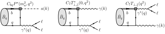
Figure 1: The diagram to the left is the main axion process $B_{q}\to\ell\ell a$ whereas the two diagrams in the centre and the right belong to the $B_{q}\to\ell\ell\gamma$ background. The single and double lines stand for the $q$ and $b$-quark, respectively. The left and central diagrams depend on off-shell form factors in the sense that the photon that emits the two leptons is off-shell. Diagrams in which the photon couples to b-quarks are not shown, but are analogous. Also diagrams with $Q_{9,10}$-operator insertions are not shown, and resemble the diagram on the right and are proportional to $C_{9}V_{\perp}$ and $C_{10}V_{\parallel}$.

2.1 Summary on $B_{q}\to\gamma^{*}$ form factors

We describe $B_{q}(p_{B})\to\gamma^{*}(k)$ transitions with off-shell photons by a set of form factors with two arguments $F^{*}(q^{2},k^{2})\equiv F^{B\to\gamma^{*}}(q^{2},k^{2})$. The first argument (here $q^{2}$) denotes the momentum transfer at the flavour-violating vertex while the second argument (here $k^{2}$) denotes the momentum of the photon. For on-shell photons, i.e. $k^{2}=0$, these form factors reduce to the well-known on-shell form factors $F(q^{2})\equiv F^{*}(q^{2},0)$ given in Eq. (A.1.3). A complete set of form factors is given by^,

$$M_{5}^{\rho}(q,k) \;\equiv\; b_{\mathrm{P}}\langle\gamma^{*}(k,\rho)|\bar{q}\gamma_{5}b|\bar{B}_{q}(p_{B})\rangle \;=\; im_{B_{q}}{R}^{\rho}\,P^{*}(q^{2},k^{2})\;,$$

$$M^{\mu\rho}_{V}(q,k) \;\equiv\; b_{\mathrm{V}}\langle\gamma^{*}(k,\rho)|\bar{q}\gamma^{\mu}b|\bar{B}_{q}(p_{B})\rangle \;=\; R_{\perp}^{\mu\rho}\,V_{\perp}^{*}(q^{2},k^{2})\;,$$

$$M^{\mu\rho}_{A}(q,k) \;\equiv\; b_{\mathrm{V}}\langle\gamma^{*}(k,\rho)|\bar{q}\gamma^{\mu}\gamma_{5}b|\bar{B}_{q}(p_{B})\rangle \;=\; R_{\parallel}^{\mu\rho}\,V_{\parallel}^{*}(q^{2},k^{2})+{R}^{\mu\rho}_{\mathbb{L}}V_{\mathbb{L}}^{*}(q^{2},k^{2})+\frac{2{R}^{\mu\rho}_{P}}{\hat{q}^{2}}P^{*}(q^{2},k^{2})\;,$$

$$M^{\mu\rho}_{T}(q,k) \;\equiv\; b_{\mathrm{T}}\langle\gamma^{*}(k,\rho)|\bar{q}iq_{\nu}\sigma^{\mu\nu}b|\bar{B}_{q}(p_{B})\rangle \;=\; R_{\perp}^{\mu\rho}\,T_{\perp}^{*}(q^{2},k^{2})\;,$$

$$M^{\mu\rho}_{T_{5}}(q,k) \;\equiv\; b_{\mathrm{T}}\langle\gamma^{*}(k,\rho)|\bar{q}iq_{\nu}\sigma^{\mu\nu}\gamma_{5}b|\bar{B}_{q}(p_{B})\rangle \;=\; -(R_{\parallel}^{\mu\rho}\,T_{\parallel}^{*}(q^{2},k^{2})+{R}^{\mu\rho}_{\mathbb{L}}T_{\mathbb{L}}^{*}(q^{2},k^{2}))\;,$$ (2.1)

where $\hat{q}^{2}\equiv q^{2}/m_{B}^{2}$ throughout, $q\equiv p_{B}-k$ denotes the momentum transfer at the flavour-violating vertex, and we define the off-shell photon state $\langle\gamma^{*}(k,\rho)|$ as in Eq. (A.2). The coefficients

$$b_{\mathrm{P}} \equiv\frac{m_{b}+m_{q}}{s_{e}e}\,, b_{\mathrm{V}} \equiv-\frac{m_{B_{q}}}{s_{e}e}\,, b_{\mathrm{T}} \equiv\frac{1}{s_{e}e}\,,$$ (2.2)

depend on the sign convention, $s_{e}$, for the covariant derivative $D_{\mu}=\partial_{\mu}+s_{e}iQ_{f}eA_{\mu}$. The Lorentz tensors ${R}$ are defined by

$$R_{\perp}^{\mu\rho} \;\equiv\; \varepsilon^{\mu\rho\beta\gamma}q_{\beta}k_{\gamma}\;, R_{\parallel}^{\mu\rho}\equiv\; \frac{i}{2}(1-\hat{q}^{2})\,(m_{B_{q}}^{2}G^{\mu\rho}-\frac{(q+2k)^{\mu}{R}^{\rho}}{1-\hat{k}^{2}})\;,$$

$$R_{\mathbb{L}}^{\mu\rho} \;\equiv\; \frac{i}{2}(q^{\mu}-\frac{\hat{q}^{2}(q+2k)^{\mu}}{1-\hat{k}^{2}})\,{R}^{\rho}\;,\qquad R_{P}^{\mu\rho}\equiv\; \frac{i}{2}q^{\mu}{R}^{\rho}\;,\quad\quad{R}^{\rho}\equiv q^{\rho}-\frac{k\!\cdot\!q}{k^{2}}k^{\rho}\;,$$ (2.3)

where $G_{\alpha\beta}\equiv g_{\alpha\beta}-k_{\alpha}k_{\beta}/k^{2}$ and (kinematic) hatted quantities are divided by $m_{B_{q}}^{2}$, e.g. $\hat{k}^{2}\equiv k^{2}/m_{B}^{2}$. The matrix element satisfy the QED and the axial Ward identities

$$k_{\rho}M^{\rho}_{5}(q,k)=0\;,\quad k_{\rho}M^{\mu\rho}_{\mathrm{V},A,T,T_{5}}(q,k) =0\,, q_{\mu}\,M^{\mu\rho}_{\mathrm{A}}(q,k) =m_{B_{q}}M_{5}^{\rho}(q,k)\;.$$ (2.4)

The latter implies the relation between the pseudoscalar and one of the axial form factors which reduces the number of independent form factors down to a total of seven. At $q^{2}=0$ there are two further constraints

$$P^{*}(0,k^{2})=\hat{V}^{*}_{\mathbb{L}}(0,k^{2})\;,\quad T_{\parallel}^{*}(0,k^{2})=(1-\hat{k}^{2})T_{\perp}^{*}(0,k^{2})\;,$$ (2.5)

where $\hat{V}^{*}_{\mathbb{L}}(q^{2},k^{2})\equiv-\hat{q}^{2}/2V^{*}_{\mathbb{L}}(q^{2},k^{2})$ thereby reducing the form factors down to five. An extensive discussion including dispersion representations in the $q^{2}$ and $k^{2}$ variables, the derivation of Eq. (2.5), the limit to photon on-shell form factors, and their computation from QCD SRs are deferred to Appendix A. As an example let us quote the once-subtracted dispersion representation for the pseudoscalar form factor for

$$P^{B_{s}\to\gamma^{*}}(q^{2},k^{2}) \;=\; P^{B_{s}\to\gamma^{*}}(q^{2},k_{0}^{2})-(k^{2}-k_{0}^{2})\int_{\textrm{cut}}^{\infty}\frac{du\,\textrm{Im}_{u}[P^{B_{s}\to\gamma^{*}}(q^{2},u)]}{(u-k_{0}^{2})(u-k^{2}-i0)}$$ (2.6)

$$\;\stackrel{{\scriptstyle k_{0}^{2}\to 0}}{{=}}\; -k^{2}\int_{\textrm{cut}}^{\infty}\frac{du\,\textrm{Im}_{u}[P^{B_{s}\to\gamma^{*}}(q^{2},u)]}{u(u-k^{2}-i0)}=-k^{2}\left(\frac{2}{m_{B_{q}}}\frac{f^{\textrm{e}m}_{\phi}\,A_{0}^{B_{s}\to\phi}(q^{2})}{(m_{\phi}^{2}-k^{2})}+\dots\right)\;,$$

which simplifies for the subtraction point $k_{0}^{2}=0$. Above $f_{\phi}^{\textrm{em}}$ is the electromagnetic decay constant in the Appendix A.2 and $A_{0}$ is the pseudoscalar $B_{s}\to\phi$ form factors [29]. In the last step the dispersion relation was evaluated for the lowest term and the dots stand for terms higher in the spectrum e.g. $B_{s}\to\phi^{\prime}$ and multiple particle configurations.

The off-shell form factors in the limit of small momentum transfer at the flavour-violating vertex, $T_{\perp,\parallel,{\mathbb{L}}}^{*}(0,q^{2})$, $V_{\perp,\parallel,{\mathbb{L}}}^{*}(0,q^{2})$ and $P^{*}(0,q^{2})$ are computed in this work for the first time. The $B\to\gamma^{*}(\to\ell^{+}\ell^{-})\mathbb{V}$ differential rate, presented in Appendix B, is another example application of these off-shell form factors for searches beyond the SM. The extension of the off-shell form factors to low $k^{2}$ into the resonance region, as shown in (2.6), requires the matching to the QCD SR result. The discussion thereof is delegated to Appendix A.4 and involves, by choice, a multiple subtracted dispersion relation where additionally use is made of the on-shell form factors. Plots are shown in Figure 6. An ancillary Mathematica notebook is added to the arXiv version for reproducing the form factors. This is for example relevant for the prediction of $B\to\gamma\ell\ell$ as the two form factors $T^{*}_{\perp,\parallel}(0,k^{2})$, where $k^{2}$ is the dilepton mass, enter the description. These two form factors have also been considered in [33, 32, 34] using improved vector meson dominance.

For the on-shell form factors $B\to\gamma$ we use the next-leading-order (NLO) light-cone sum rule (LCSR) computation [35]. Note that the QCD SR result of the off-shell form factors can be used in the relevant kinematic region $(4.9\mbox{GeV})^{2}\lesssim q^{2}<m_{B_{q}}^{2}$ since thresholds are far away. The photon on-shell form factors are more challenging in this region because the light-cone expansion breaks down. They can, however, be extrapolated to this region by using a $B_{q}^{*}$ and $B_{q1}$-pole ansatz, with the residue computed from LCSR [36], supplemented with $z$-expansion corrections to account for further states.

2.2 The $B_{q}\to\ell\ell a$ differential rate

Given the effective Lagrangian in Eq. (1.1), the amplitude for $\bar{B}_{q}(p_{B})\to\ell^{+}(p_{\ell^{+}})~{}\ell^{-}(p_{\ell^{-}})~{}a(k)$ is

$${\cal A}_{\mu\mu a} =-i\frac{e^{2}Q_{\ell}}{m_{B_{q}}q^{2}}~{}\frac{k_{\mu}}{F^{A}_{bq}}~{}M^{\mu\rho}_{A}(k,q)~{}\bar{u}^{s}(p_{\ell^{-}})\gamma_{\rho}v^{r}(p_{\ell^{+}})=-i\frac{e^{2}Q_{\ell}}{F^{A}_{bq}q^{2}}~{}M^{\rho}_{5}(k,q)~{}\bar{u}^{s}(p_{\ell^{-}})\gamma_{\rho}v^{r}(p_{\ell^{+}})\,,$$ (2.7)

where ${\cal A}_{\mu\mu a}\equiv\langle\mu\mu a|-\mathscr{L}_{\textrm{int}}|\bar{B}_{q}\rangle$, $q\equiv p_{B}-k=p_{\ell^{+}}+p_{\ell^{-}}$ and $Q_{\ell}=-1$ denotes the lepton charge. After squaring this amplitude, summing over fermion spins, and integrating over the unobserved axion momentum, the differential rate in the invariant mass of the final-state leptons, $q^{2}$, becomes

$$\frac{d\Gamma}{dq^{2}}(B_{q}\to\ell\ell a)=\frac{\alpha^{2}}{48\pi m_{B_{q}}}\frac{\lambda^{1/2}_{\gamma}\,(\lambda^{(a)}_{B_{q}})^{3/2}}{|F_{bq}^{A}|^{2}}\frac{2m_{\ell}^{2}+q^{2}}{q^{8}}|P^{*}(m_{a}^{2},q^{2})|^{2}\;,$$ (2.8)

where $\lambda_{\gamma}\equiv\lambda(q^{2},m_{\ell}^{2},m_{\ell}^{2})$, $\lambda^{(a)}_{B_{q}}\equiv\lambda(m_{B_{q}}^{2},q^{2},m_{a}^{2})$, and $\lambda(x,y,z)\equiv x^{2}+y^{2}+z^{2}-2xy-2xz-2yz$ is the Källèn function. For our work it is sufficient to approximate $m_{a}\to 0$.

2.3 The $B_{q}\to\ell\ell\gamma$ differential rate

The relevant part of the effective SM Lagrangian

$$\mathscr{L}_{\text{SM}}=\frac{4G_{\mathrm{F}}}{\sqrt{2}}\lambda_{t}\sum_{i=7,9,10}\left(C_{i}Q_{i}+C_{i}^{\prime}Q^{\prime}_{i}\right)+\text{h.c.}\,,$$

where $\lambda_{t}\equiv V_{tb}^{*}V_{tq}$ and

$$Q_{7}= \frac{s_{e}e}{16\pi^{2}}m_{b}\bar{b}\sigma^{\mu\nu}q_{L}F_{\mu\nu}\,, Q_{9[10]}= \frac{e^{2}}{16\pi^{2}}(\bar{b}\gamma^{\mu}q_{L})(\bar{\ell}\gamma_{\mu}[\gamma_{5}]\ell)\,,$$ (2.9)

$q_{L,R}\equiv(1\mp\gamma_{5})/2q$, and $Q^{\prime}_{7,9,10}$ is obtained from $Q_{7,9,10}$ by the replacements $L\to R$ and $m_{b}\to m_{q}$. Upon using the helicity vector completeness relation (A.19), the $\bar{B}_{q}(p_{B})\to\ell^{+}(p_{\ell^{+}})~{}\ell^{-}(p_{\ell^{-}})~{}\gamma(k)$ amplitude ($q\equiv p_{B}-k=p_{\ell^{+}}+p_{\ell^{-}}$, $\lambda_{B_{q}}\equiv\lambda(m_{B_{q}}^{2},q^{2},0)$ and $r_{q}\equiv-is_{e}e/2\,\lambda^{1/2}_{B_{q}}$)

$${\cal A}_{\mu\mu\gamma(\lambda)} =\langle\mu\mu\gamma(\lambda)|-\mathscr{L}_{\textrm{SM}}|\bar{B}_{q}\rangle=\frac{\alpha G_{\textrm{F}}\lambda_{t}}{\sqrt{2}\pi}r_{q}\sum_{\lambda=\perp,\parallel}({\cal A}^{V}_{\lambda}L^{V}_{\lambda}+{\cal A}^{A}_{\lambda}L^{A}_{\lambda})\;,$$ (2.10)

can be factored into a leptonic $L^{V,A}_{\lambda}=\epsilon^{*}_{\nu}(q,\lambda)\bar{u}(p_{\ell^{-}})\gamma^{\nu}[\gamma_{5}]\bar{v}(p_{\ell^{+}})$ and the hadronic helicity amplitude follows from the Hamiltonian with where the leptons are removed up to a normalisation factor. For the effective axial leptons one finds

$$r_{q}{\cal A}^{A}_{\pm} \;=\; \langle\gamma(\pm)|\frac{(C_{10}\pm C^{\prime}_{10})}{2}\bar{s}\gamma^{\mu}1(-\gamma_{5})b|\bar{B}_{q}\rangle\epsilon^{\mu}(q,\pm)$$

$$\;=\; \pm\frac{(C_{10}\pm C^{\prime}_{10})}{2b_{V}}M^{V(A)}_{\mu\rho}(q,k)\epsilon^{*\mu}(k,\pm)\epsilon^{\rho}(q,\pm)\;,$$ (2.11)

and for the vector ones

$$r_{q}{\cal A}^{V}_{\pm} \;=\; r_{q}{\cal A}^{A}_{\pm}\Big{|}_{C_{10}\to C_{9}}-\frac{2Q_{\ell}m_{b}}{q^{2}}\left(\pm\frac{(C_{7}\pm\frac{m_{q}}{m_{b}}C^{\prime}_{7})}{2b_{T}}\overline{M}^{T_{(5)}}_{\mu\rho}(q,k)\epsilon^{*\mu}(k,\pm)\epsilon^{\rho}(q,\pm)\right)$$ (2.12)

where $\overline{M}^{T_{(5)}}_{\mu\rho}(q,k)\equiv M^{T_{(5)}}_{\mu\rho}(q,k)+M^{T_{(5)}}_{\mu\rho}(k,q)$ takes into account both types of diagrams in Figure 1. Explicit parameterisations of the polarisation vectors and some more explanations can be found in Appendix A.1.3. Using the (common) convention $\sqrt{2}{\cal A}_{\perp,\parallel}={\cal A}_{+}\mp{\cal A}_{-}$ one gets ($Q_{\ell}=-1$)

$$\begin{split}{\cal A}^{V}_{{\perp,\parallel}}=&\frac{1}{m_{B_{q}}}(C_{9}\pm C^{\prime}_{9})V_{\perp,\parallel}^{*}(q^{2},0)+\frac{2m_{b}}{q^{2}}(C_{7}\pm\frac{m_{q}}{m_{b}}C_{7}^{\prime})\overline{T}_{\perp,\parallel}(q^{2})\;,\\[5.0pt] {\cal A}^{A}_{\perp,\parallel}=&\frac{1}{m_{B_{q}}}(C_{10}\pm C^{\prime}_{10})V_{\perp,\parallel}^{*}(q^{2},0)\,.\end{split}$$ (2.13)

Above

$$\begin{split}\overline{T}_{\perp}(q^{2})&=T_{\perp}^{*}(q^{2},0)+T_{\perp}^{*}(0,q^{2})\,,\\ \overline{T}_{\parallel}(q^{2})&=T_{\parallel}^{*}(q^{2},0)+T_{\parallel}^{*}(0,q^{2})/(1-q^{2}/m_{B_{q}}^{2})=T_{\parallel}^{*}(q^{2},0)+T_{\perp}^{*}(0,q^{2})\,.\end{split}$$ (2.14)

The last equality relates $T_{\parallel}^{*}(0,q^{2})$ to $T_{\perp}^{*}(0,q^{2})$, see Appendix A.1.6 and footnote 8 just before Eq. (A.1.1). Above we omitted the contribution from photons radiated off final-state muons, because these are obtained from the $B_{q}\to\mu\mu$ rates using PHOTOS, cf., Ref. [37]. Going slightly lower in $q^{2}$ would necessitate the inclusion of broad charmonium resonances [38, 39]. For an overview of other non form-factor matrix elements see for instance Refs. [38, 32].

After integrating over the unobserved photon momentum, the differential rate for the radiative mode $B_{q}\to\ell\ell\gamma$ reads

$$\frac{d\Gamma}{dq^{2}}(B_{q}\to\ell\ell\gamma)=\frac{\alpha^{3}G_{F}^{2}|\lambda_{t}|^{2}}{768\pi^{4}}\frac{\lambda^{1/2}_{\gamma}\lambda^{3/2}_{B_{q}}}{m_{B_{q}}^{3}q^{2}}\left(c_{A}(|{\cal A}^{A}_{\perp}|^{2}+|{\cal A}^{A}_{\parallel}|^{2})+c_{V}(|{\cal A}^{V}_{\perp}|^{2}+|{\cal A}^{V}_{\parallel}|^{2})\right)\;,$$ (2.15)

and $c_{V}\equiv(q^{2}+2m_{\ell}^{2})$, $c_{A}\equiv(q^{2}-4m_{\ell}^{2})$ are effectively the squared leptonic helicity amplitudes.

2.4 $B_{q}\to\mu\mu a$ and $B_{q}\to\mu\mu\gamma$ close to the kinematic endpoint

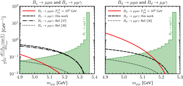
Figure 2: Comparison of the axionic decay mode $B_{q}\to\mu\mu a$ (red solid lines) and the radiative $B_{q}\to\mu\mu\gamma$ modes (black lines). The left panel shows the $B_{s}$ case while the right the $B_{d}$ case. For the axion predictions $F_{bq}^{A}=10^{6}$ GeV is assumed as a reference value. The different black lines are the photon predictions with different form factor treatments (see legend and main text). In green are bins of the two-body $B_{q}\to\mu\mu$ rate including radiation from final-state muons. To better compare the $B_{s}$ and $B_{d}$ cases, all rates are normalised to their respective two-body decay $B_{q}\to\mu\mu$, which is why the $B_{d}\to\mu\mu a$ line appears enhanced with respect to the $B_{s}\to\mu\mu a$ one.

To illustrate the relative importance between the SM background $B_{q}\to\mu\mu\gamma$ and the $B_{q}\to\mu\mu a$ signal we take as a reference value for the flavour-violating coupling $F^{A}_{bq}=10^{6}$ GeV. In Figure 2, we show the differential rate normalised with respect to the two-body decay width

$$\frac{1}{\Gamma(B_{q}\to\mu\mu)}\frac{d\Gamma(B_{q}\to\mu\mu X)}{dm_{\mu\mu}}\,,$$

where $X=a,\gamma$, $m_{\mu\mu}^{2}\equiv q^{2}$. In the left panel, we show the predictions for the $B_{s}$ decays and in the right the corresponding ones for the $B_{d}$ case. The binned (green) predictions are the $B_{q}\to\mu\mu$ rates including photon radiation from the final-state muons using PHOTOS (see Ref. [37]). The red solid lines are the rates from the axion mode for the reference value $F_{bq}^{A}=10^{6}$ GeV (note that the relative enhancement between left and the right panel is due to the normalization, which carries a different CKM suppression.). The black lines are the $B_{q}\to\mu\mu\gamma$ predictions when the photon does not originate from muon bremsstrahlung. They depend on the treatment of the non-perturbative input, i.e., the hadronic form factors introduced in Section 2.1. In all cases, we use the same perturbative input, namely the SM Wilson coefficients $C_{7}^{\text{eff}}$, $C_{9}^{\text{eff}}$ and $C_{10}$ evaluated at the hadronic $B_{q}$ scale. We obtain $C_{10}$ from Ref. [37] and use flavio [40] to evaluate $C_{7}^{\text{eff}}$ and $C_{9}^{\text{eff}}$.

We show the results of three different approaches of estimating the relevant hadronic form factors:

• Dashed line: the QCD SR form factor computation discussed in Section 2.1 and Appendix A,

• Dotted line: the quark-model approach of Ref. [32],

• Dashed-dotted line: the pole-dominance approach supplemented by experimental data and heavy-quark effective theory of Ref. [41]. It is specific to the $B_{s}$ case (left panel).

The agreement of the predictions is rather crude. For $q^{2}\approx(4.9\mbox{GeV})^{2}$, our prediction is about a factor of three larger than the quark model [32] and about a factor of two smaller than the pole-dominance approximation [41]. The disagreement with the quark model is not surprising as the method is designed for low $q^{2}$ and, unlike in our work, no additional input is employed to constrain the residua of the leading poles near the kinematic endpoint. The agreement of the form factors themselves at lower $q^{2}$, which we do not show, is much better. The comparison with the pole-dominance approach [41] has two major components. The difference in the $B^{*}_{q}$-residue and the fact that the effect of $B_{q1}$-resonance is neglected in Ref. [41] cf. Appendix A.5.1. While it is important to understand the origin of the discrepancy in light of a possible measurement of the radiative decay, the discrepancy does not play a significant role in obtaining a bound on the axion couplings $F^{A}_{bq}$, which we derive in the next section.

3 Sensitivity at LHCb

In this section we recast the LHCb analysis of Ref. [23] to obtain an estimate for the current and future sensitivity of LHCb to probe the flavour-violating couplings $F^{A}_{bs}$ and $F^{A}_{bd}$. We first discuss, in Section 3.1, how we extract the backgrounds by rescaling the original LHCb analysis, and derive the expected number of events in each bin for a given luminosity. We then describe, in Section 3.2, our statistical method and provide the recast of the present data and the sensitivity study for future runs. Our main results are summarised in Tables 2 and 3.

3.1 Rescaling the LHCb analysis

The $B_{s}\to\mu\mu$ analysis of LHCb in Ref. [23] makes use of datasets collected at different LHC runs, with luminosities $\overline{{\cal L}}_{7}=1.0$ fb^-1 from $7$ TeV, $\overline{{\cal L}}_{8}=2.0$ fb^-1 from $8$ TeV, and $\overline{{\cal L}}_{13}=1.4$ fb^-1 from $13$ TeV runs. Under the SM hypothesis, a total number of $62$ $B_{s}\to\mu\mu$ events and $6.7$ $B_{d}\to\mu\mu$ events are expected in this analysis in the full range of boosted-decision-trees (BDT) and the signal window ($m_{\mu\mu}\in[5.2,5.445]$ GeV). Since the BDT discrimination is flat one expects half of these events to pass the BDT $>0.5$ selection. For this BDT selection, LHCb supplies a plot with backgrounds, which we use to extract their numerical values. By combining the expected number of $B_{q}\to\mu\mu$ events in the SM with the SM branching-fraction predictions, we extract a universal rescaling factor, $r\approx 0.079$, via

$$\begin{split}N_{B_{d}}&=\underbrace{(\epsilon\,2f_{d})}_{\equiv r}\times~{}\overline{\text{BR}}^{B_{d}\to\mu\mu(n\gamma)}_{[5.2~{}\text{GeV}-5.445\,\text{GeV}]}\times\!\!\sum_{i=7,8,13}\sigma_{b,i}\overline{\cal L}_{i}\,,\\ N_{B_{s}}&=r\times\frac{f_{s}}{f_{d}}\times~{}\overline{\text{BR}}^{B_{s}\to\mu\mu(n\gamma)}_{[5.2~{}\text{GeV}-5.445\,\text{GeV}]}\times\!\!\sum_{i=7,8,13}\sigma_{b,i}\overline{\cal L}_{i}\,.\end{split}$$ (3.1)

In these equations, $i$ labels the $\sqrt{s}$ run and $\sigma_{i}$ is the corresponding $b$-quark production cross section in the acceptance of LHCb. The latter has been measured by LHCb for $\sqrt{s}=7,13$ TeV, $\sigma_{b,7}=72$ $\mu$b and $\sigma_{b,13}=144$ $\mu$b [44]. For $\sigma_{b,8}$ we linearly rescale the $7$ TeV value ($\sigma_{b,8}=8/7\sigma_{b,7}$). $f_{d}$ and $f_{s}$ are the fragmentation ratios of $b$-quarks that are produced at LHCb and fragment into $B_{d}$ and $B_{s}$, respectively. We absorb $f_{d}$ in the rescaling factor, $r$, and use the ratio $f_{s}/f_{d}$ to obtain $N_{B_{s}}$. This ratio has been measured by the LHCb collaboration to be $f_{s}/f_{d}=0.259\pm 0.015$ [45]. Finally, $\epsilon$ summarises the experimental efficiencies and all other global rescaling factors, which we absorb into the definition of $r$.

The quantities $\overline{\text{BR}}$’s in Eq. (3.1) are the respective branching ratios in the signal window. This includes the effect of photon radiation from muons [46, 37], which LHCb simulates with PHOTOS. The overline in the branching-ratio prediction indicates that the partial width is divided by the width of the heavy mass eigenstate ($\Gamma^{H}_{B_{s}},~{}\Gamma^{H}_{B_{d}}$) to obtain the branching fraction. In this way the effect of $B_{q}$-mixing is included [47, 37]. This is relevant for the $B_{s}$ system, but much less so for the $B_{d}$ system. This is numerically equivalent to LHCb’s treatment of the effective lifetime, cf. Eq. (1) in Ref. [23]).

LHCb’s BDT $>0.5$ selection covers the $m_{\mu\mu}\in[4.9~{}\text{GeV},m_{B_{s}}]$ region in bins of $50$ MeV. We apply the same universal rescaling factor, $r$, to rescale the predictions of all $B_{q}\to\mu\mu a$ and $B_{q}\to\mu\mu\gamma$ branching fractions for all $m_{\mu\mu}$ bins. This is a good approximation as there are no triggers or similar thresholds that significantly change the rescaling over this invariant-mass range. In the next section, we present the sensitivity of this analysis to probe the flavour-violating $F^{A}_{bs}$ and $F^{A}_{bd}$ axion couplings in future runs of LHCb by rescaling the $13$ TeV dataset. We denote the corresponding effective total luminosity by

$${\cal L}=\overline{\cal L}_{7}+\overline{\cal L}_{8}+{\cal L}_{13}\,.$$ (3.2)

At a given total luminosity, ${\cal L}$, the expected number of events at a given $m_{\mu\mu}$-bin (Bin_k) then is

$$\begin{split}N_{k}[F^{A}_{bs},&F^{A}_{bd}]=N_{\text{Bin}_{k}}^{\text{BKG,analysis}}\frac{\text{SL}({\cal L})}{\text{SL}(\overline{\cal L})}\\ &+\left(\overline{\text{BR}}_{\text{Bin}_{k}}[B_{d}\to\mu\mu(n\gamma)]+\overline{\text{BR}}_{\text{Bin}_{k}}[B_{d}\to\mu\mu\gamma]+\overline{\text{BR}}_{\text{Bin}_{k}}[B_{d}\to\mu\mu a]\right)\,r\,\text{SL}({\cal L})\\ &+\left(\overline{\text{BR}}_{\text{Bin}_{k}}[B_{s}\to\mu\mu(n\gamma)]+\overline{\text{BR}}_{\text{Bin}_{k}}[B_{s}\to\mu\mu\gamma]+\overline{\text{BR}}_{\text{Bin}_{k}}[B_{s}\to\mu\mu a]\right)\,r\,\frac{f_{s}}{f_{d}}\text{SL}({\cal L})\,,\end{split}$$ (3.3)

with shorthands $\overline{\cal L}\equiv\overline{\cal L}_{7}+\overline{\cal L}_{8}+\overline{\cal L}_{13}=4.4\,{\mathrm{f}b}^{-1}$ and $\text{SL}({\cal L})\equiv\sigma_{b,7}\overline{\cal{L}}_{7}+\sigma_{b,8}\overline{\cal{L}}_{8}+\sigma_{b,13}({\cal L}-\overline{\cal{L}}_{7}-\overline{\cal{L}}_{8})$ . The quantity $N_{\text{Bin}_{i}}^{\text{BKG,analysis}}$ is the expected total number of background events that do not originate from the radiative decay in the given bin. We obtain $N_{\text{Bin}_{i}}^{\text{BKG,analysis}}$ by digitising and integrating the plot of LHCb’s BDT $>0.5$ selection. In Eq. (3.3) we kept separate the rate from photon emission from muons ($B_{q}\to\mu\mu(n\gamma)$) and the rate from photon emissions from the initial state ($B_{q}\to\mu\mu\gamma$). In principle, the amplitudes interfere but the interference is tiny close to the $B_{q}$ threshold and we thus neglect it.

3.2 Recast and sensitivity analysis

To compute the sensitivity of the LHCb analysis in probing $F^{A}_{bs}$ and $F^{A}_{bd}$, we must combine the information of all $m_{\mu\mu}$ bins and include statistical and systematic uncertainties. We neglect the subdominant experimental systematic uncertainties but will include the theory uncertainties associated to the form factors entering the three-body rates. In what follows we always either turn on $F^{A}_{bs}$ or $F^{A}_{bd}$, i.e., but will not let them float simultaneously.

Each $m_{\mu\mu}$ bin corresponds to an independent counting experiment that obeys Poisson statistics. Exclusion limits on $F^{A}_{bq}$ are then obtained from a joined Poisson (Log)Likelihood. For a sufficiently large number of events, Poisson statistics are well described by Gaussian statistics and the Poisson (Log)Likelihood is equivalent to a $\chi^{2}$ function of the NP parameter, i.e., $F^{A}_{bq}$:

$$\chi^{2}(F^{A}_{bq})=\sum_{i,j}(N_{i}-N^{\text{obs}}_{i})(V_{\text{cov}}^{-1})_{ij}(N_{j}-N^{\text{obs}}_{j})\,,$$ (3.4)

with $i$ numbering the bins and $q=s,\,d$. $N_{i}=N_{i}(F^{A}_{bq})$ denotes the total number of events (background plus signal) for the value $F^{A}_{bq}$ in a given bin, whereas $N^{\text{obs}}_{i}$ is the observed number of events. For the recast we use the actual number of events observed by LHCb, read off from Figure 1 in Ref. [23]. To project the sensitivity for future LHCb runs we set $N^{\text{obs}}_{i}$ to the number of events expected in the SM. The covariance matrix, $V_{\text{cov}}$, incorporates statistical and systematic uncertainties in a way that we discuss below. If we neglect systematic uncertainties, this matrix is diagonal and only contains the squared Poisson variances, $V_{\text{cov}}=V_{\text{stat}}$ with $(V_{\text{stat}})_{ij}=\delta_{ij}N_{i}$. We have explicitly checked, that for the data samples considered here, the Poisson (Log-)Likelihood is always very well approximated by the $\chi^{2}$.

To incorporate systematic/theory uncertainties we follow the commonly used approach of Ref. [48]. Theory uncertainties are then treated as Gaussian uncertainties smearing the expectation values of the underlying Poisson probability distribution functions. We can then obtain the limits on $F^{A}_{bq}$ by generating Monte-Carlo events based on the joined Poisson likelihood after smearing the expectation values by the (correlated) systematic errors. If the measurement is well-described by Gaussian statistics (as in our case) and the systematic uncertainties are small with respect to the statistical ones, this treatment of uncertainties is equivalent to adding the statistical and systematic errors in quadrature in $V_{\text{cov}}$.

In our case the main systematic uncertainties are due to the form factors that enter the radiative $B_{q}\to\mu\mu\gamma$ and the $B_{q}\to\mu\mu a$ rate. Since the uncertainties in the form factors originate in part from uncertainties in input parameters like $m_{b}$ and $\langle\bar{q}q\rangle$ that are $q^{2}$-independent, the predicted number of events among different bins are correlated. Therefore, the full covariance matrix for the case in which the axion has a coupling $F^{A}_{bq}$ is not diagonal and decomposes into

$$V_{\text{cov}}=V_{\text{stat}}+V_{\gamma}+\frac{1}{(F^{A}_{bq})^{4}}V^{q}_{a}+\frac{1}{(F^{A}_{bq})^{2}}V^{q}_{a-\gamma}\,.$$ (3.5)

Here, $(V_{\text{stat}})_{ij}=\delta_{ij}N_{i}$ are the statistical uncertainties, while the matrices $V_{\gamma}$, $V^{q}_{a}$, and $V^{q}_{a-\gamma}$ describe the correlated errors among the predictions of various rates over the bins. Aside from trivial functional dependencies on global rescaling factors, e.g., luminosity, we can determine them once and for all by generating Monte-Carlo events in which we vary the parameters on which the form factors depend. In practice we use the mean values of the $z$-expansion fit (of degree four) and their covariance matrix (see Appendix A.5.3) to determine each piece of $V_{\text{cov}}$. Using the covariance matrices we obtain the $90\%$ Confidence Level (CL) exclusion limit on $|F^{A}_{bq}|$, i.e. $\chi^{2}(F^{A}_{bq,90\%})-\chi^{2}_{\text{min}}=1.64$.

	$\boldsymbol{B_{s}\to\mu\mu a}$		$\boldsymbol{B_{d}\to\mu\mu a}$
	sys+stat	stat only	sys+stat	stat only
$\chi^{2}_{\text{min}}$	$15.2$	$15.4$	$14.8$	$15.1$
$|F^{A}_{bq,\text{best-fit}}|\times 10^{-5}$ [GeV]	$4.3$	$4.8$	$5.0$	$5.5$
$|F^{A}_{bq,\text{90\%}}|\times 10^{-5}$ [GeV]	$>2.4$	$>2.6$	$>3.0$	$>3.2$

Table 2: The results of recasting LHCb’s analysis [23] to test flavour-violating couplings of the axion to $B_{s}$ ($F^{A}_{bs})$ and $B_{d}$ ($F^{A}_{bd}$). The analysis employs a total of $4.4$ fb^-1 of data from runs at $7$, $8$, and $13$ TeV. In the columns labelled “sys+stat” we combine statistical and theory uncertainties, while in the columns labelled “stat only” we neglect the latter. We see that presently the bounds are dominated by statistical uncertainties. When computing the $\chi^{2}$ we sum over the ten first bins of the analysis, i.e., $m_{\mu^{+}\mu^{-}}\in[4.9~{}\text{GeV},m_{B_{s}}]$. For every case we list the values of the $\chi^{2}_{\text{min}}$ and the corresponding best-fit value for $|F^{A}_{bq}|$. The values of $\chi^{2}_{\text{min}}$ should be compared with the $\chi^{2}$ value of the SM, $\chi^{2}_{\text{SM}}=15.7$. The axion best-fit values are thus in roughly $1\sigma$ agreement with the SM. $|F^{A}_{bq,90\%}|$ are the resulting $90\%$ CL exclusion limits.

First, we recast the observed data of LHCb’s analysis [23] in which ${\cal L}=\overline{\cal L}=4.4$ fb^-1. The measurement is dominated by statistical uncertainties, but for purposes of illustration we show both the bounds when combining statistical and systematic theory errors and the bounds when only the statistical uncertainty is included. In the $\chi^{2}$ we include the first ten bins of the LHCb analysis. The observed data are in good agreement with the SM expectation. Indeed, we find that the $\chi^{2}$ of the SM divided by the ten degrees of freedom of the $\chi^{2}$ (d.o.f.) is $\chi_{\text{SM}}/{\text{d.o.f.}}=1.6$. The best-fit points for the axion lies roughly $1\sigma$ off the SM. In Table 2 we list the best-fit points with their corresponding $\chi^{2}_{\text{min}}$, as well as the resulting $90\%$ CL exclusion limits on $|F^{A}_{bs}|$ and $|F^{A}_{bd}|$.

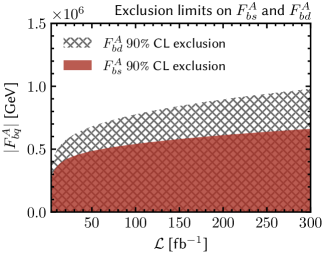
Figure 3: Projected sensitivity of LHCb to probe the flavour-violating axion couplings $F^{A}_{bs}$ (filled red region) and $F^{A}_{bd}$ (hatched region) as a function of the total integrated luminosity. Shown are the $90\%$ CL exclusion limits assuming that the observed number of events will be the same as predicted in the SM hypothesis.

		$\boldsymbol{B_{s}\to\mu\mu a}$		$\boldsymbol{B_{d}\to\mu\mu a}$
		$|F^{A}_{bs}|\times 10^{-5}$ [GeV]		$|F^{A}_{bd}|\times 10^{-5}$ [GeV]
${\cal L}$ [fb-1]		sys+stat	stat only	sys+stat	stat only
$10$		$3.6$	$3.9$	$4.9$	$5.2$
$30$		$4.5$	$5.3$	$6.2$	$7.1$
$50$		$4.8$	$6.1$	$6.8$	$8.2$
$100$		$5.4$	$7.3$	$7.7$	$9.8$
$300$		$6.6$	$9.7$	$9.8$	$13$

Table 3: Projected $90\%$ CL exclusion limits on the flavour-violating couplings of the axion to $B_{s}$ ($F^{A}_{bs}$) and $B_{d}$ ($F^{A}_{bd}$) as a function of the integrated luminosity at LHCb. In the columns labelled “sys+stat” we combine statistical and theory uncertainties, while in the columns labelled “stat only” we neglect the latter.

Next we make projections for future runs of LHCb. As discussed in Section 3.1, to this end we rescale the $13$ TeV events assuming LHCb will collect a total of $300$ fb^-1. To compute the sensitivity we assume that LHCb will observe exactly the number of events expected from the SM. Therefore, the best-fit point always corresponds to observing zero events from axion decays and $\chi^{2}_{\text{min}}=0$. For the projection study we present the results both when only statistical uncertainties are considered and when they are folded with the correlated theory uncertainties. In Figure 3 we show the resulting $90\%$ CL exclusion limit on $|F^{A}_{bs}|$ (left panel) and $|F^{A}_{bd}|$ (right panel) as a function of the total luminosity. In addition, the limits for some indicative luminosities are listed in Table 3.

Note that the limit from the actual recast is weaker than the expected limit under the background-only hypothesis. More precisely, if we consider the case ${\cal L}=4.4$ fb^-1 and set $N_{i}^{\text{obs}}=N_{i}^{\text{SM}}$ (as we do for the projection study) we find for the statistics-only case $|F_{bs,90\%}^{A}|<{3.0}\cdot 10^{5}$ GeV and $|F_{bd,90\%}^{A}|<{4.0}\cdot 10^{5}$ GeV. In comparison, the corresponding exclusion limits of the recast (table 3) are slightly weaker. The origin of this difference is mainly an excess of roughly $10$ events in the first bin of the current LHCb $B_{s}\to\mu\mu$ analysis, which can be fitted by the best-fit point of an axion signal. However, as discussed in the recast the excess is not statistically significant and the best-fit point of the axion is within $1\sigma$ of the SM.

4 Summary and Outlook

In this article we have proposed a novel method to probe flavour-violating couplings of the QCD axion to $b$-quarks at the LHC, exploiting the di-muon datasets collected for the $B_{q}\to\mu\mu$ analyses. To this end, we have computed the relevant differential decay rates for the decay of a $B_{q}$-meson to muons and an axion $B_{q}\to\mu\mu a$ [Eq. (2.8)] and the radiative decay $B_{q}\to\mu\mu\gamma$ [Eq. (2.15)], which is a background to the former process.

These rates depend on non-perturbative $B_{q}\to\gamma^{(*)}$ form factors, which we have discussed from a general viewpoint, computed with QCD sum rules (at zero flavour-violating momentum transfer). To the best of our knowledge this is the first discussion of the complete set of form factors, for the dimension-six effective Hamiltonian ${\cal H}_{\textrm{eff}}^{b\to(d,s)}$, supplemented with an explicit computation of all form factors in Appendix A. The uncertainty of this leading order computation is estimated to be around $25\%$ and could benefit from radiative corrections which is, however, an elaborate task. We extend these form factors to the low-lying resonance region of unflavoured vector mesons by using a multiple subtracted dispersion relation cf. Appendix A.4. A Mathematica notebook is appended to the arXiv version. Besides being useful for axion searches these form factors are also the ingredients for other light BSM particle (e.g. dark photon) searches. In addition, we have exposed the relation between the introduced basis and the standard $B\to V$ basis through the dispersion representation in Appendix A.2, which interrelates form-factor properties of the two bases. A further application of the off-shell form factor formalism is to consider the charged case with $q^{2},k^{2}>0$ which is needed to describe $B\to\ell^{+}\ell^{-}\ell^{\prime}\nu$. We postpone this task to a future study as this involves discriminating charges and dealing with contact terms but note that these decays has recently been described by different groups [49, 50, 51, 52] using different approaches.

With these decay rates we performed a recast using available LHCb data and estimated the sensitivity to $B_{q}\to\mu\mu a$ at present and future runs, taking into account the SM background $B_{q}\to\mu\mu\gamma$. We find that present data constrain the relevant axion couplings $F^{A}_{bd}\,(F^{A}_{bs})$ to be larger than $3.0(2.4)\cdot 10^{5}\,{\mbox{GeV}}$ at 90% CL [Table 2], while the full LHCb dataset will probe scales of the order of $10^{6}\,{\mbox{GeV}}$ in both $b\to d$ and $b\to s$ transitions (Table 3).

For stable axions, these results should be compared with the ones derived from $B$-meson decays with missing energy. In the case of $b\to s$ transitions, the data from the BaBar collaboration on $B\to K^{*}\nu\overline{\nu}$ provide constraints that are roughly two orders of magnitude stronger than the ones from our LHCb recast of $B_{s}\to\mu\mu a$, cf. Table 1. For the case of $b\to d$ transitions, the BaBar constraints are roughly of the same order than the ones that LHCb can obtain in upcoming runs. Nevertheless, the combination with the corresponding ATLAS and CMS analyses of $B_{q}\to\mu\mu$ may improve the bounds significantly. In Appendix B we made further use of the off-shell form factors to estimate the strength of LHCb to search for light, Beyond the Standard Model, vectors.

While it is remarkable that the LHC can play a role in constraining couplings of the QCD axion, the analysis of $B_{q}\to\mu\mu a$ that we have presented here can be relevant for other extensions of the SM with light neutral particles with flavour-violating couplings. Since the $B_{q}\to\mu\mu a$ analysis is inclusive, it can be extended to search for light BSM particles even if they decay within the detector. For example, an ALP that decays promptly to, for instance, photons may be subject to cuts on additional photons in the analyses of $B\to K(a\to\gamma\gamma)$ at the $B$-factories and thus evade detection, while it would be kept in the $B_{q}\to\mu\mu(a\to\gamma\gamma)$ samples at the LHC. Therefore, the analysis that we have presented here complements axion searches in rare meson decays with missing energy at B-factories, and can play an important role in constraining flavour-violating couplings of light particles.

Appendix A The $B_{q}\to\gamma^{*}$ Form Factors

The standard $B_{q}\to V$ matrix elements (ME), where $V=\rho^{0},\omega,\phi\ldots$ is a vector meson, hold some analogy with the $B_{q}\to\gamma^{*}$ ones. However, the difference is that the analogue of the vector-meson mass is the photon off-shell momentum which is a variable rather than a constant. Hence the MEs are functions of two variables and this leads to a more involved analytic structure. In this paper we restricted ourselves to the kinematic region $q^{2}\in[(4.9\mbox{GeV})^{2},m_{B_{q}}^{2}]$, where the form factors (FFs) can be expected to dominate over long-distance contributions.

This appendix is structured as follows. Firstly, we define and state relation and limits of the FFs in Section A.1, the link with the $B\to V$ basis is discussed in Section A.2, the QCD SR computation of the off-shell FFs follows in Section A.3 and finally we turn to the FF-parametrisation and fits in Section A.5. Note, that sections A.1, A.2 and A.5 are independent of the method of computation.

Form Factor	$P^{*}(0,k^{2})$	$T_{\parallel}^{*}(0,k^{2})=(1-\hat{k}^{2})T_{\perp}^{*}(0,k^{2})$	$V,T_{\perp,\parallel}(q^{2})=V^{*},T^{*}_{\perp,\parallel}(q^{2},0)$
Mode	$B_{s}\to\ell\ell a$	$B_{s}\to\ell\ell\gamma$	$B_{s}\to\ell\ell\gamma$
Poles $q^{2},k^{2}$	$m_{\phi}^{2},m_{\Upsilon}^{2}$	$m_{\phi}^{2},m_{\Upsilon}^{2}$	$m_{B^{*}_{q}}^{2},m_{B_{q1}}^{2}$
Defined in Eqs.	(2.1, A.1.1)	(2.1, A.1.1)	(A.1.3)
Graph in Figure 1	(left)	(centre)	(right)
Other notation	$-$	$F_{TV}(0,k^{2})=F_{TA}(0,k^{2})$[53, 32]	$F_{V,A},\,F_{TV,A}(q^{2},0)$[53, 32]

Table 4: Overview of FFs referencing definitions, graphs, and analytic structure. The latter defines the region of validity of the computation. Long-distance contributions are relevant in other kinematic regions [32, 38]. For $B_{d}\to\gamma^{*}$, $m_{\phi}^{2}$ is to be replaced by $m_{\rho,\omega}^{2}$ above.

A.1 Definition of $B\to\gamma^{(*)}$ form factors

We introduce a complete set of off-shell FFs which is related to the standard $B\to V$ basis [54, 29] via dispersion relations, cf. Section A.2. On a technical level this appendix extends previous work [53, 32], in that we discuss the full set of seven vector and tensor FFs and not only those needed for the SM transition. The complete basis is for example useful for other invisible particle searches such as the dark photon. The off-shell FFs are not to be confused with the on-shell FFs which have received more attention in the literature [53, 33, 32, 55]. An overview of the on- and off-shell FFs used for this paper are shown in the diagrams in Figure 1 and contrasted in Table 4.

A.1.1 The complete basis of seven off-shell form factors $F^{*}(q^{2},k^{2})$

We introduce the FFs with two momentum squares $q^{2}$ and $k^{2}$ collectively as $F^{*}(q^{2},k^{2})\equiv F^{B\to\gamma^{*}}(q^{2},k^{2})$. The first argument (here $q^{2}$) denotes the momentum transfer at the flavour-violating vertex while the second argument (here $k^{2}$) denotes the momentum of the photon emitted at low energies.

We introduce a new off-shell basis via a dispersion representation based on the standard $B\to V$ basis [54, 29]. Below we state the basis before turning to the construction in Section A.2. The absence of unphysical singularities in the matrix element enforces relations between FFs which we discuss in some detail. We will refer to this circumstance as “regularity” for short.

The complete set of FFs were already introduced in the main text in Eq. (2.1) and reproduced here for convenience^,

$$M_{5}^{\rho} \;\equiv\; b_{\mathrm{P}}\langle\gamma^{*}(k,\rho)|\bar{q}\gamma_{5}b|\bar{B}_{q}(p_{B})\rangle \;=\; im_{B_{q}}{R}^{\rho}\,P^{*}(q^{2},k^{2})$$

$$M^{\mu\rho}_{V} \;\equiv\; b_{\mathrm{V}}\langle\gamma^{*}(k,\rho)|\bar{q}\gamma^{\mu}b|\bar{B}_{q}(p_{B})\rangle \;=\; +R_{\perp}^{\mu\rho}\,V_{\perp}^{*}(q^{2},k^{2})\;,$$

$$M^{\mu\rho}_{A} \;\equiv\; b_{\mathrm{V}}\langle\gamma^{*}(k,\rho)|\bar{q}\gamma^{\mu}\gamma_{5}b|\bar{B}_{q}(p_{B})\rangle \;=\; +(R_{\parallel}^{\mu\rho}\,V_{\parallel}^{*}(q^{2},k^{2})+{R}^{\mu\rho}_{\mathbb{L}}V_{\mathbb{L}}^{*}(q^{2},k^{2})+{R}^{\mu\rho}_{P}V^{*}_{P}(q^{2},k^{2}))\;,$$

$$M^{\mu\rho}_{T} \;\equiv\; b_{\mathrm{T}}\langle\gamma^{*}(k,\rho)|\bar{q}iq_{\nu}\sigma^{\mu\nu}b|\bar{B}_{q}(p_{B})\rangle \;=\; +R_{\perp}^{\mu\rho}\,T_{\perp}^{*}(q^{2},k^{2})\;,$$

$$M^{\mu\rho}_{T_{5}} \;\equiv\; b_{\mathrm{T}}\langle\gamma^{*}(k,\rho)|\bar{q}iq_{\nu}\sigma^{\mu\nu}\gamma_{5}b|\bar{B}_{q}(p_{B})\rangle \;=\; -(R_{\parallel}^{\mu\rho}\,T_{\parallel}^{*}(q^{2},k^{2})+{R}^{\mu\rho}_{\mathbb{L}}T_{\mathbb{L}}^{*}(q^{2},k^{2}))\;,$$ (A.1)

where $b_{\mathrm{P}}\equiv\left(\frac{m_{b}+m_{q}}{s_{e}e}\right)$, $b_{\mathrm{V}}\equiv\left(-\frac{m_{B_{q}}}{s_{e}e}\right)$, $b_{\mathrm{T}}\equiv\left(\frac{1}{s_{e}e}\right)$, the momentum transfer is $q\equiv p_{B}-k$ and the off-shell photon state $\langle\gamma^{*}(k,\rho)|$ is defined through

$$\langle\gamma^{*}(k,\rho)|O(0)|B\rangle\equiv-ies_{e}\int d^{4}xe^{ik\cdot x}\langle 0|Tj^{\rho}(x)O(0)|B\rangle\;,$$ (A.2)

where $j^{\rho}=\sum_{f}Q_{f}\bar{f}\gamma^{\rho}f$ is the electromagnetic current.

$$R_{\perp}^{\mu\rho} \;\equiv\; \varepsilon^{\mu\rho\beta\gamma}q_{\beta}k_{\gamma}\;, R_{\parallel}^{\mu\rho}\equiv\; \frac{i}{2}(1-\hat{q}^{2})\,(m_{B_{q}}^{2}G^{\mu\rho}-\frac{(q+2k)^{\mu}{R}^{\rho}}{1-\hat{k}^{2}})\;,$$

$$R_{\mathbb{L}}^{\mu\rho} \;\equiv\; \frac{i}{2}(q^{\mu}-\frac{\hat{q}^{2}(q+2k)^{\mu}}{1-\hat{k}^{2}})\,{R}^{\rho}\;,\qquad R_{P}^{\mu\rho}\equiv\; \frac{i}{2}q^{\mu}{R}^{\rho}\;,\quad\quad{R}^{\rho}\equiv q^{\rho}-\frac{k\!\cdot\!q}{k^{2}}k^{\rho}\;,$$ (A.3)

are Lorentz tensors with convenient properties (cf. below) and hereafter

$$\hat{k}^{2}\equiv\frac{k^{2}}{m_{B_{q}}^{2}}\;,\quad\hat{q}^{2}\equiv\frac{q^{2}}{m_{B_{q}}^{2}}\;.$$ (A.4)

The photon transverse tensor, $k^{\alpha}G_{\alpha\beta}=0$, is

$$G_{\alpha\beta}\equiv g_{\alpha\beta}-\frac{k_{\alpha}k_{\beta}}{k^{2}}\;,$$ (A.5)

and it is noted that ${R}^{\rho}=q_{\mu}G^{\mu\rho}$ (A.1.1).

A.1.2 Constraints for off-shell Form Factors

The QED Ward identity holds off-shell in the form

$$k_{\rho}M^{\mu\rho}_{\mathrm{V},A,T,T_{5}}=0\;,$$ (A.6)

without contact term since the weak operator is neutral in the total electric charge. Note that Eq. (A.6) is automatically satisfied in our parametrisation since $k_{\rho}{R}^{\mu\rho}_{\perp,\parallel,{\mathbb{L}},P}=0$. The non-singlet axial Ward identity for $M^{\mu\rho}_{\mathrm{A}}$ assumes the form

$$q_{\mu}\,M^{\mu\rho}_{\mathrm{A}}=m_{B_{q}}M_{5}^{\rho}\;,$$ (A.7)

which in turn holds without contact term since the electromagnetic current is invariant under non-singlet axial rotations. Eq. (A.7), upon using $q_{\mu}R^{\mu\rho}_{\perp,\parallel,{\mathbb{L}}}=0$, implies that

$$V_{P}^{*}(q^{2},k^{2})=\frac{2}{\hat{q}^{2}}P^{*}(q^{2},k^{2})\;.$$ (A.8)

Regularity enforces constraints on the FFs defined in (A.1.1). There are two constraints at $q^{2}=0$ and $k^{2}=m_{B_{q}}^{2}$ respectively. The Ward identity (A.8) enforces

$$P^{*}(0,k^{2})=\hat{V}^{*}_{\mathbb{L}}(0,k^{2})\;,$$ (A.9)

where $\hat{V}^{*}_{\mathbb{L}}$ is implicitly defined by

$$V^{*}_{\mathbb{L}}(q^{2},k^{2})\equiv-\frac{2}{\hat{q}^{2}}\hat{V}^{*}_{\mathbb{L}}(q^{2},k^{2})\;.$$ (A.10)

The second constraint is

$$T_{\parallel}^{*}(0,k^{2})=(1-\hat{k}^{2})T_{\perp}^{*}(0,k^{2})\;.$$ (A.11)

There are two further constraints due to the parametrisation of the form factors at $k^{2}=m_{B_{q}}^{2}$

$$(1-\hat{q}^{2})V_{\parallel}^{*}(q^{2},m_{B_{q}}^{2})+\hat{q}^{2}V_{\mathbb{L}}^{*}(q^{2},m_{B_{q}}^{2}) \;=\; 0\;,$$

$$(1-\hat{q}^{2})T_{\parallel}^{*}(q^{2},m_{B_{q}}^{2})+\hat{q}^{2}T_{\mathbb{L}}^{*}(q^{2},m_{B_{q}}^{2}) \;=\; 0\;,$$ (A.12)

which are of a similar type as the $A_{0}^{B\to V}(0)=A_{3}^{B\to V}(0)$ cf. (A.39). Whereas the constraints (A.9) and (A.1.2) are imposed by the FF-parametrisation (avoiding spurious kinematic singularities), (A.11) is of algebraic origin cf. Section A.1.6 for the derivation.

A.1.3 The four photon on-shell form factors $F(q^{2})\equiv F^{*}(q^{2},0)$

We next turn to the case where the low-energy photon is on-shell; $k^{2}=0$. We introduce the commonly used shorthand

$$F(q^{2})\equiv F^{*}(q^{2},0)\;,\quad\text{for}\quad F\in\{P,V_{\perp,\parallel,{\mathbb{L}}},T_{\perp,\parallel,{\mathbb{L}}}\}\;,$$ (A.13)

(or $F^{B\to\gamma}(q^{2})\equiv F^{B\to\gamma^{*}}(q^{2},0)$). The basic physics idea is that the absence of the photon’s zero helicity component implies the vanishing the pseudoscalar FF and the zero helicity part of the vector FFs. We may define the helicity amplitude for $B\to\mu\mu\gamma$ by

$${\cal A}_{\lambda\lambda^{\prime}}^{X}\propto M_{X}^{\mu\rho}\omega^{*}_{\mu}(q,\lambda)\epsilon^{*}_{\rho}(k,\lambda^{\prime})\;.$$ (A.14)

One then obtains the two $B\to\gamma\mu\mu$ helicity amplitudes

$${\cal A}^{A}_{0} \;=\; {\cal A}_{00}^{A}\stackrel{{\scriptstyle k^{2}\to 0}}{{\propto}}V_{\parallel}-V_{\mathbb{L}}\;,\quad {\cal A}^{A}_{t} \;=\; {\cal A}_{t0}^{A}\stackrel{{\scriptstyle k^{2}\to 0}}{{\propto}}P\;,\quad {\cal A}^{T_{5}}_{0} \;=\; {\cal A}_{00}^{T_{5}}\stackrel{{\scriptstyle k^{2}\to 0}}{{\propto}}T_{\parallel}-T_{\mathbb{L}}\;,$$ (A.15)

and the $\pm$ direction obey

$${\cal A}^{A}_{+} \;=\; {\cal A}_{++}^{A}\stackrel{{\scriptstyle k^{2}\to 0}}{{\propto}}V_{\parallel}-V_{\perp}\;,\quad {\cal A}^{A}_{-} \;=\; {\cal A}_{--}^{A}\stackrel{{\scriptstyle k^{2}\to 0}}{{\propto}}V_{\parallel}+V_{\perp}\;,\quad$$ (A.16)

and the formulae for the vector $V$ as well as the tensors $T,T_{5}$ are similar. The common definition

$${\cal A}^{A}_{\perp,\parallel}\equiv\frac{1}{\sqrt{2}}\left({\cal A}^{A}_{+}\mp{\cal A}^{A}_{-}\right)\propto V_{\perp,\parallel}\;,$$ (A.17)

explains the notation. In order to obtain these results it is useful to choose an explicit helicity vector parameterisations. E.g. in the $B_{q}$-meson restframe (e.g. [Eq.15] in [56])

$$\epsilon(k,0) \;=\; (v,0,0,\sqrt{k^{2}+v^{2}})/\sqrt{k^{2}}\;,\quad \epsilon(k,t) \;=\; k/\sqrt{k^{2}}\;,\quad \!\!\!\!\!\!\!\!\!\!\!\!k\;=\;(\sqrt{k^{2}+v^{2}},0,0,v)\;,$$

$$\omega(q,0) \;=\; (-v,0,0,\sqrt{q^{2}+v^{2}})/\sqrt{q^{2}}\;,\quad \omega(q,t) \;=\; q/\sqrt{q^{2}}\;,\quad \!\!\!\!\!\!\!\!\!\!\!\!q\;=\;(\sqrt{q^{2}+v^{2}},0,0,-v)\;,$$

$$\epsilon(k,\pm) \;=\; \omega(q,\mp)=(0,\mp 1,i,0)/\sqrt{2}\;,\quad \epsilon(\perp,\parallel) \;=\; \frac{\epsilon(+)\mp\epsilon(-)}{\sqrt{2}}\;,$$ (A.18)

where the velocity is given by $v\equiv|\vec{k}|=\lambda^{1/2}(m_{B_{q}}^{2},q^{2},k^{2})/(2m_{B_{q}})$ and $k\to k^{\mu}$ is the Lorentz-index convention in the formulae above. This helicity basis is useful since

$$g_{\mu\nu}=\sum_{\lambda=t,0,\pm}\epsilon_{\mu}^{*}(\lambda)\epsilon_{\nu}(\lambda^{\prime})G^{\lambda\lambda^{\prime}}=\sum_{\lambda=t,0,\perp,\parallel}\epsilon_{\mu}^{*}(\lambda)\epsilon_{\nu}(\lambda^{\prime})G^{\lambda\lambda^{\prime}}$$ (A.19)

with $G^{\lambda\lambda^{\prime}}=\textrm{diag}(1,-1,-1,-1)$ and the first entry denotes the $t$-component. Second, in the limit $k^{2}\to 0$, $\epsilon^{*}(k,0)\propto k$, and this enforces,

$$\lim_{k^{2}\to 0}\epsilon^{*}_{\rho}(k,0)M^{\mu\rho}_{A,T_{5}}=0\;,$$ (A.20)

since it is equivalent to the QED Ward identity (A.6). Eqs. (A.15, A.20) lead to the constraints

$$V_{\parallel}(q^{2})=V_{\mathbb{L}}(q^{2})\;,\quad T_{\parallel}(q^{2})=T_{\mathbb{L}}(q^{2})\;,\quad P(q^{2})=0\;,$$ (A.21)

and reduces the seven FFs of Eq. (A.1.1) to four. Alternatively one can infer the constraints (A.21) from the regularity of the matrix elements as $k^{2}\to 0$. The regularity condition and the helicity arguments are clearly related.

For completeness we give the explicit $k^{2}\to 0$ basis [38, 55]

$$M^{\mu}_{V} \;\equiv\; b_{\mathrm{V}}\langle\gamma(\epsilon(k))|\bar{q}\gamma^{\mu}b|\bar{B}_{q}(p_{B})\rangle \;=\; +P_{\perp}^{\mu}\,V_{\perp}(q^{2})\;,$$

$$M^{\mu}_{A} \;\equiv\; b_{\mathrm{V}}\langle\gamma(\epsilon(k))|\bar{q}\gamma^{\mu}\gamma_{5}b|\bar{B}_{q}(p_{B})\rangle \;=\; +P_{\parallel}^{\mu}\,V_{\parallel}(q^{2})\;,$$

$$M^{\mu}_{T} \;\equiv\; b_{\mathrm{T}}\langle\gamma(\epsilon(k))|\bar{q}iq_{\nu}\sigma^{\mu\nu}b|\bar{B}_{q}(p_{B})\rangle \;=\; +P_{\perp}^{\mu}\,T_{\perp}(q^{2})\;,$$

$$M^{\mu}_{T_{5}} \;\equiv\; b_{\mathrm{T}}\langle\gamma(\epsilon(k))|\bar{q}iq_{\nu}\sigma^{\mu\nu}\gamma_{5}b|\bar{B}_{q}(p_{B})\rangle \;=\; -P_{\parallel}^{\mu}\,T_{\parallel}(q^{2})\;,$$ (A.22)

where

$$P_{\perp}^{\mu} \;\equiv\; \epsilon^{*}_{\rho}{R}_{\perp}^{\mu\rho}=\varepsilon^{\mu\rho\beta\gamma}\epsilon^{*}_{\rho}q_{\beta}k_{\gamma}\;\quad P_{\parallel}^{\mu}\equiv\; \epsilon^{*}_{\rho}({R}_{\parallel}^{\mu\rho}+{R}_{\mathbb{L}}^{\mu\rho})=i\,(q\!\cdot\!k\,\epsilon^{*\,\mu}-q\!\cdot\!\epsilon^{*}\,k^{\mu})\;.$$ (A.23)

Relation to the standard $B\to V$ basis

We consider it worthwhile to comment on some aspects in the standard basis of $B\to V$ FFs e.g. [29]. The $k^{2}\to 0$ limit is then akin to $m_{V}\to 0$. The relations $V_{\parallel}(q^{2})-V_{\mathbb{L}}(q^{2})=T_{\parallel}(q^{2})-T_{\mathbb{L}}(q^{2})=0$ implies

$${\cal V}^{B\to V}_{2}(q^{2})=(1-\hat{q}^{2}){\cal V}^{B\to V}_{3}(q^{2})+{\cal O}(m_{V})\;,$$

$$T^{B\to V}_{2}(q^{2})=(1-\hat{q}^{2})T^{B\to V}_{3}(q^{2})+{\cal O}(m_{V})\;.$$ (A.24)

Such relations were noted previously. Firstly, in the $B\to V$ context in Ref. [57] in Appendix A and around Eq. [5] in Ref. [31], where it is argued that the relation has to hold in order to cancel a kinematic $1/m_{V}$-factor. Second for $B\to\gamma$ ($m_{V}=0$) they were previously reported in Ref. [53] as a consequence of regularity.

A.1.4 The five form factors $F^{*}(0,k^{2})$ at zero flavour-violating momentum transfer

In the process $B_{q}\to\ell\ell X$, with $X$ a light BSM particle, the limit in which the flavour-violating momentum transfer goes to zero, i.e., $q^{2}=0$, corresponds to the case of zero or small mass of $X$. In this limit the two constraints in Eqs. (A.9) and (A.11) reduce the number of independent FFs from seven to five.

The matrix elements, at $q^{2}=0$,the become

$$M^{\mu\rho}_{V} \;\equiv\; b_{\mathrm{V}}\langle\gamma^{*}(k,\rho)|\bar{q}\gamma^{\mu}b|\bar{B}_{q}(p_{B})\rangle \;\to\; +{R}_{\perp}^{\mu\rho}\,V_{\perp}^{*}(0,k^{2})\;,$$

$$M^{\mu\rho}_{A} \;\equiv\; b_{\mathrm{V}}\langle\gamma^{*}(k,\rho)|\bar{q}\gamma^{\mu}\gamma_{5}b|\bar{B}_{q}(p_{B})\rangle \;\to\; +({R}_{\parallel}^{\mu\rho}\,V_{\parallel}^{*}(0,k^{2})+i\frac{(2k+q)^{\mu}}{1-\hat{k}^{2}}{R}^{\rho}\,P^{*}(0,k^{2}))\;,$$

$$M^{\mu\rho}_{T} \;\equiv\; b_{\mathrm{T}}\langle\gamma^{*}(k,\rho)|\bar{q}iq_{\nu}\sigma^{\mu\nu}b|\bar{B}_{q}(p_{B})\rangle \;\to\; +{R}_{\perp}^{\mu\rho}\,T_{\perp}^{*}(0,k^{2})\;,$$

$$M^{\mu\rho}_{T_{5}} \;\equiv\; b_{\mathrm{T}}\langle\gamma^{*}(k,\rho)|\bar{q}iq_{\nu}\sigma^{\mu\nu}\gamma_{5}b|\bar{B}_{q}(p_{B})\rangle \;\to\; -({R}_{\parallel}^{\mu\rho}\,(1-\hat{k}^{2})T_{\perp}^{*}(0,k^{2})+\frac{i}{2}q^{\mu}{R}^{\rho}T_{\mathbb{L}}^{*}(0,k^{2}))\;,$$ (A.25)

where Eqs.  (A.9,A.11) and $2k\!\cdot\!q|_{q^{2}=0}=m_{B_{q}}^{2}-k^{2}$ have been used. At $q^{2}=0$ the constraints (A.1.2) imply

$$V_{\parallel}^{*}(0,m_{B_{q}}^{2})=2P^{*}(0,m_{B_{q}}^{2})\;,\quad T_{\parallel}^{*}(0,m_{B_{q}}^{2})=0\;.$$ (A.26)

With $T_{\mathbb{L}}^{*}(0,m_{B_{q}}^{2})$ finite, the last constraint is obeyed trivially by (A.11).

A.1.5 Counting form factors

type$\backslash$ $J^{P}$	$\#$	$1^{-}$	$1^{+}$	$1^{+}$	$0^{-}$
$F^{*}(q^{2},k^{2})$	$\!\!7\!$	$V_{\perp}^{*}(q^{2},k^{2})$	$V_{\parallel}^{*}(q^{2},k^{2})$	$\hat{V}_{\mathbb{L}}^{*}(q^{2},k^{2})$	$P^{*}(q^{2},k^{2})$
		$T_{\perp}^{*}(q^{2},k^{2})$	$T_{\parallel}^{*}(q^{2},k^{2})$	$T_{\mathbb{L}}^{*}(q^{2},k^{2})$
$F(q^{2})\equiv$	$\!\!4\!$	$V_{\perp}(q^{2})$	$V_{\parallel}(q^{2})$	$V_{\mathbb{L}}(q^{2})=V_{\parallel}(q^{2})$	$P(q^{2})=0$
$F^{*}(q^{2},0)$		$T_{\perp}(q^{2})$	$T_{\parallel}(q^{2})$	$T_{\mathbb{L}}(q^{2})=T_{\parallel}(q^{2})$
$F^{*}(0,k^{2})$	$\!\!5\!$	$V_{\perp}^{*}(0,k^{2})$	$V_{\parallel}^{*}(0,k^{2})$	$\hat{V}_{\mathbb{L}}^{*}(0,k^{2})=P^{*}(0,k^{2})$	$P^{*}(0,k^{2})$
		$T_{\perp}^{*}(0,k^{2})$	$T_{\parallel}^{*}(0,k^{2})=(1\!-\!\hat{k}^{2})T_{\perp}^{*}(0,k^{2})$	$T_{\mathbb{L}}^{*}(0,k^{2})$

Table 5: The $J^{P}=0^{+}$ FF vanishes by parity conservation of QCD. Generally, there are seven independent $F^{*}(q^{2},k^{2})$ FFs (light-blue) with two constraints $\hat{V}_{\mathbb{L}}^{*}(0,k^{2})=P^{*}(0,k^{2})$ (A.9) and $T^{*}_{\parallel}(0,k^{2})=(1-\hat{k}^{2})T^{*}_{\perp}(0,k^{2})$ (A.11). For the photon on-shell case, $F(q^{2})\equiv F^{*}(q^{2},0)$, there are four independent FFs (light-red) and the reduction is due to the absence of the photon $0$-helicity component. At zero flavour-violating momentum there are five independent FFs (light-green), due to the two constraints mentioned above. For the computation of the $B\to\ell\ell\gamma$ SM rate, the following five FFs are sufficient $\{V_{\perp,\parallel}(q^{2}),T_{\perp,\parallel}(q^{2}),T_{\perp}^{*}(0,k^{2})\}$.

Since the last few sections were a bit involved with many steps we summarise the classification in Table 5. In general there are seven FFs for the $B\to 1^{-}$ transition. In the photon on-shell case this reduces to four because the photon comes with two polarisations only. In the case of zero flavour-violating momentum transfer the two general constraints (A.9, A.11) reduce this number from seven to five.

A.1.6 Derivation of $T_{\parallel}^{B\to\gamma^{*}}(0,k^{2})=(1-\hat{k}^{2})T_{\perp}^{B\to\gamma^{*}}(0,k^{2})$

At last we turn to the derivation of the relation (A.11). We may choose to proceed by uncontracting the $B\to V$ matrix element, first in $q^{\nu}$ (A.1.1)

$$b_{\mathrm{T}}\langle V(\eta(k))|\bar{q}\sigma^{\mu\nu}\gamma_{5}b|\bar{B}_{q}(p)\rangle=x_{0}\eta^{*}\!\cdot\!p\frac{k^{[\mu}p^{\nu]}}{q\cdot k}+x_{1}\eta^{*\,[\mu}k^{\nu]}+x_{2}\eta^{*\,[\mu}p^{\nu]}=\eta^{*\,\alpha}x_{\alpha}^{\mu\nu}\;,$$ (A.27)

with shorthands $x_{i}=x_{i}(q^{2},k^{2})$, $p=p_{B}$, $\eta$ is the polarisation vector of a massive vector boson and square brackets denote antisymmetrisation in the respective indices. The corresponding uncontracted $B\to\gamma^{*}$ matrix element then reads

$$M^{\mu\nu\rho}_{T_{5}}\equiv b_{\mathrm{T}}\langle\gamma^{*}(k,\rho)|\bar{q}\sigma^{\mu\nu}\gamma_{5}b|\bar{B}_{q}(p)\rangle=X_{0}{R}^{\rho}\frac{k^{[\mu}p^{\nu]}}{q\cdot k}+X_{1}g^{\rho[\mu}k^{\nu]}+X_{2}(g^{\rho[\mu}p^{\nu]}-\frac{k^{\rho}}{k^{2}}k^{[\mu}p^{\nu]})\;,$$ (A.28)

where

$$M^{\mu\nu\rho}_{T_{5}}=c\,G^{\rho\alpha}x_{\alpha}^{\mu\nu}\;,$$ (A.29)

with $c$ some $i$-independent kinematic function ($X_{i}=cx_{i}$) which is irrelevant for our purposes. The appearance of the tensor $G^{\rho\alpha}$ can be understood from the viewpoint of a dispersion relation cf. Section A.2 or and footnote 12. Regularity enforces at $k\cdot q\propto 1-\hat{k}^{2}-\hat{q}^{2}\to 0$ ,

$$X_{0}(q^{2},m_{B_{q}}^{2}-q^{2})=0\;,$$ (A.30)

and at $k^{2}\to 0$ we have

$$X_{0}(q^{2},0)+X_{2}(q^{2},0)=0\;.$$ (A.31)

These two constraints are generally valid.

We may make the connection with our basis by identifying

$$M^{\mu\rho}_{T_{5}}=iq_{\nu}M^{\mu\nu\rho}_{T_{5}}\;,\quad M^{\mu\rho}_{T}=-\frac{i}{2}(iq_{\nu})\epsilon^{\mu\nu}_{\phantom{\mu\nu}\mu^{\prime}\nu^{\prime}}M^{\mu^{\prime}\nu^{\prime}\rho}_{T_{5}}\;,$$ (A.32)

to obtain

$$T_{\perp}^{*}(q^{2},k^{2}) \;=\; -(X_{1}(q^{2},k^{2})+X_{2}(q^{2},k^{2}))\;,$$

$$T_{\parallel}^{*}(q^{2},k^{2}) \;=\; -\frac{1-\hat{k}^{2}}{1-\hat{q}^{2}}\,(X_{1}(q^{2},k^{2})+X_{2}(q^{2},k^{2}))+\frac{\hat{q}^{2}}{1-\hat{q}^{2}}\,(X_{1}(q^{2},k^{2})-X_{2}(q^{2},k^{2}))\;,$$

$$T_{\mathbb{L}}(q^{2},k^{2}) \;=\; (X_{2}(q^{2},k^{2})-X_{1}(q^{2},k^{2}))+2\frac{1-\hat{k}^{2}}{1-\hat{k}^{2}+\hat{q}^{2}}\,X_{0}(q^{2},k^{2})\;.$$ (A.33)

There are two consequences of this equation. Since $X_{1}$ and $X_{2}$ are free from poles at $q^{2}=0$ one gets (A.11),

$$T_{\parallel}^{*}(0,k^{2})=(1-\hat{k}^{2})T_{\perp}^{*}(0,k^{2})\;,$$ (A.34)

and by inserting (A.31) into $T_{\mathbb{L}}^{*}$ one deduces that $T_{\mathbb{L}}(q^{2})=T_{\parallel}(q^{2})$, which we derived earlier cf. (A.21). This confirms the earlier observation that the regularity conditions in $k^{2}\to 0$ are equivalent to the previously mentioned helicity argument. The derivation of relations (A.34) achieves the purpose of this section. The relation (A.34) appears for any set of FF and reads $T_{1}^{B\to V}(0)=T_{2}^{B\to V}(0)$ in the notation of [54, 29] and has been derived in the off-shell FF context in reference [53].

A.2 Relation of the $B\to\gamma^{*}$- and $B\to V$-basis through the dispersion relation

In this appendix we make the link between the $B\to V$- and the $B\to\gamma^{*}$-FFs through the dispersion relations. This is an instructive exercise and we will be able to recover properties of the $B\to\gamma^{*}$ FFs from the $B\to V$-ones. Our argumentation remains true if one considers any intermediate state (e.g. two pseudoscalar particles in a $P$-wave) as long as its quantum number, $J^{PC}=1^{--}$, is equal to the one of the photon. This is the case since the properties follows from the general decomposition and the fact that any such state can be interpolated by the electromagnetic current in the LSZ formalism. In addition the dispersion representation may be useful for improving the fit ansatz of these FFs.

For our purposes it is convenient to first write the $B\to V$ FFs [54, 29] in the following form

$$c^{(q)}_{V}\langle V(k,\eta)|\bar{q}\gamma^{\mu}(1\mp\gamma_{5})b|\bar{B}(p_{B})\rangle(-m_{B_{q}}) \;=\; \;\;P_{1}^{\mu}\,\bar{\cal V}_{1}^{B\to V}(q^{2})\pm\sum_{i=2,3,P}P_{i}^{\mu}\bar{\cal V}_{i}^{B\to V}(q^{2})\;,$$

$$c^{(q)}_{V}\langle V(k,\eta)|\bar{q}iq_{\nu}\sigma^{\mu\nu}(1\pm\gamma_{5})b|\bar{B}(p_{B})\rangle \;=\; \;\;P_{1}^{\mu}T_{1}^{B\to V}(q^{2})\pm\sum_{i=2,3}P_{i}^{\mu}T_{i}^{B\to V}(q^{2})\;,$$ (A.35)

where $\eta$ is the vector-meson polarisation, $P_{i}^{\mu}$ are Lorentz vectors

$$P_{P}^{\mu}=i(\eta^{*}\cdot q)q^{\mu}\;, P_{1}^{\mu}= 2\epsilon^{\mu}_{\phantom{x}\alpha\beta\gamma}\eta^{*\alpha}k^{\beta}q^{\gamma}\;,$$ (A.36)

$$P_{2}^{\mu}=i(1\!-\!\hat{k}^{2})\{m_{B_{q}}^{2}\eta^{*\mu}\!-\!\frac{(\eta^{*}\!\cdot\!q)}{1-\hat{k}^{2}}(k+p_{B})^{\mu}\}\;,\qquad P_{3}^{\mu}= i(\eta^{*}\!\cdot\!q)\{q^{\mu}\!-\!\frac{\hat{q}^{2}}{1\!-\!\hat{k}^{2}}(k+p_{B})^{\mu}\}\;,$$

where in (A.35) but not (A.36) $k^{2}=m_{V}^{2}$ is assumed, and

$$c^{(d)}_{\omega}=-c^{(d)}_{\rho^{0}}=\sqrt{2}\;,\quad c^{(s)}_{\phi}=1\;,$$ (A.37)

($c^{(u)}_{\omega}=c^{(u)}_{\rho_{0}}=\sqrt{2}$ are not used) take into account the composition of the vector mesons’ wave-functions, $|\rho_{0}[\omega]\rangle\approx(|\bar{u}u\rangle\mp|\bar{d}d\rangle)/\sqrt{2}$ and $|\phi\rangle\approx|\bar{s}s\rangle$. The correspondence of $\bar{\cal V}^{B\to V}_{1,2,3,P}$ with the more traditional FFs $A^{B\to V}_{0,1,2,3}$ (e.g. [29]) and $V^{B\to V}$ is as follows

$$\bar{\cal V}_{P}^{B\to V}(q^{2})=\frac{2\hat{m}_{V}}{\hat{q}^{2}}A_{0}^{B\to V}(q^{2})\;,\quad\bar{\cal V}_{1}^{B\to V}(q^{2})=\frac{V^{B\to V}(q^{2})}{1+\hat{m}_{V}}\;,\quad\bar{\cal V}_{2}^{B\to V}(q^{2})=\frac{A_{1}^{B\to V}(q^{2})}{1-\hat{m}_{V}}\;,$$

$$\bar{\cal V}_{3}^{B\to V}(q^{2})=\frac{1-\hat{m}_{V}}{\hat{q}^{2}}A_{2}^{B\to V}(q^{2})-\frac{1+\hat{m}_{V}}{\hat{q}^{2}}A_{1}^{B\to V}(q^{2})\equiv\frac{-2\hat{m}_{V}}{\hat{q}^{2}}A_{3}^{B\to V}(q^{2})\;,$$ (A.38)

where $\hat{m}_{V}\equiv m_{V}/m_{B_{q}}$. The analogue of the two ($q^{2}\!=\!0$) constraints (A.9, A.11) are

$$A^{B\to V}_{3}(0)=A^{B\to V}_{0}(0)\;,\quad T^{B\to V}_{1}(0)=T^{B\to V}_{2}(0)\;,$$ (A.39)

respectively. The constraint (A.1.2) does not apply since $m_{V}^{2}\neq m_{B_{q}}^{2}$.

As stated above the relation between the FFs becomes apparent in the dispersion representation (cf. the textbook [58] or the recent review [59]). A specific example is chosen for illustration,

$$M_{T_{5}}^{\mu\rho} \;=\; -ib_{\mathrm{T}}\int d^{4}xe^{ik\cdot x}\langle 0|Tj^{\rho}(x)\bar{q}iq_{\nu}\sigma^{\mu\nu}\gamma_{5}b(0)|\bar{B}_{q}\rangle$$

$$\;=\; \sum_{i=2,3}\,\int^{\infty}_{u_{\textrm{low}}}\frac{\rho_{T_{i}}(q^{2},u)\,du}{u-k^{2}-i0}(-G^{\rho}_{\phantom{\rho}\alpha})P_{i}^{\mu\alpha}+\textrm{subtractions}\;,$$ (A.40)

where $u_{\textrm{low}}=(m_{P_{1}}+m_{P_{2}})^{2}$, and $V\to P_{1}+P_{2}$ is the lowest decay channel (e.g. $\rho^{0}\to\pi^{+}+\pi^{-}$ for $B_{q}=B_{d}$). Note, that the appearance of the tensor $G^{\rho}_{\phantom{\rho}\alpha}$ (A.5) goes hand in hand with the QED Ward identity constraint.

In order to further illustrate we resort to the narrow width approximation (NWA) which can be improved by introducing a finite decay width or better multiparticle states of stable particles (cf. remark at beginning this section). With the NWA

$$\sum_{\lambda=-1,0,1}\eta_{\rho}^{*}(k,\lambda)\eta_{\alpha}(k,\lambda)=\left(-g_{\rho\alpha}+\frac{k_{\rho}k_{\alpha}}{m_{V}^{2}}\right)\big{|}_{m_{V}^{2}=k^{2}}=(-G_{\rho\alpha})\;,$$ (A.41)

and the spectral or discontinuity function $\rho_{T_{i}}(q^{2},u)$ assumes the simple form

$$\rho_{T_{i}}(q^{2},u)=\delta(u-m_{\rho}^{2})r^{\rho}_{T_{i}}(q^{2})+\delta(u-m_{\omega}^{2})r^{\omega}_{T_{i}}(q^{2})+\dots\;,$$ (A.42)

where the dots stand for higher states in the spectrum. The residua $r^{V}_{T_{i}}$ are then given by

$$r^{V}_{T_{i}}=-m_{V}f^{\textrm{em}}_{V}/|c^{(d,s)}_{V}|^{2}\,T^{B\to V}_{i}(q^{2})\;,$$ (A.43)

where $f^{\textrm{em}}_{V}$ is a conveniently normalised matrix element

$$(c^{(d,s)}_{V})^{*}\langle 0|j_{\mu}|V(k,\eta)\rangle=m_{V}f^{\textrm{em}}_{V}\eta_{\mu}\;,$$ (A.44)

of the electromagnetic current and the vector meson. In particular

$$f^{\textrm{em}}_{\rho_{0}}=(Q_{d}-Q_{u})f_{\rho_{0}}=-f_{\rho_{0}}\;,\quad f^{\textrm{em}}_{\omega}=(Q_{d}+Q_{u})f_{\omega}=\frac{1}{3}f_{\omega}\;,\quad f^{\textrm{em}}_{\phi}=Q_{s}f_{\phi}=-\frac{1}{3}f_{\phi}\;.$$ (A.45)

Rewriting our parametrisation (A.1.1), in compact form,

$$M_{T_{5}}^{\mu\rho}=\sum_{J=\parallel,{\mathbb{L}}}R_{J}^{\mu\rho}T^{B\to\gamma^{*}}_{J}(q^{2},k^{2})\;,$$ (A.46)

and equating with (A.2) we are able to identify the two bases

$$R_{J}^{\mu\rho}\omega_{Ji}(q^{2},k^{2})=P_{i}^{\mu\alpha}(-G^{\rho}_{\phantom{\rho}\alpha})\;,$$ (A.47)

where $\omega_{Ji}$ is, by construction, a matrix with diagonal entries

$$\omega_{\perp 1}(q^{2},k^{2})=2\;,\quad\omega_{\parallel 2}(q^{2},k^{2})=2\frac{1-\hat{k}^{2}}{1-\hat{q}^{2}}\;,\quad\omega_{{\mathbb{L}}3}(q^{2},k^{2})=2\;,\quad\omega_{PP}(q^{2},k^{2})=2\;,$$ (A.48)

only. Of course we could have chosen any other basis at the cost of having a non-diagonal $\omega$-matrix but we feel that this is an economic way.

Let us make the dispersion representation more concrete by clarifying what the subtraction terms mean in (A.2). Whether or not the $B\to\gamma^{*}$ FFs does require a subtraction is practically not important since it is advantageous to do so anyway as the on-shell FF, which provides the subtraction information, is well-known and also physical. One may write

$$T_{J}^{B\to\gamma^{*}}(q^{2},k^{2}) \;=\; T_{J}^{B\to\gamma^{*}}(q^{2},k_{0}^{2})+\omega_{Ji}\,(k^{2}-k_{0}^{2})\int^{\infty}_{u_{\textrm{low}}}\frac{\,\rho_{T_{i}}(q^{2},u)\,du}{(u-k_{0}^{2}-i0)(u-k^{2}-i0)}\;,$$ (A.49)

where $J=\perp,{\mathbb{L}},P$ and $i=1,3,P$ with $\omega_{Ji}$ defined above and the same formula applies for $T^{*}_{J}\to V^{*}_{J}$ and $\rho_{T_{i}}\to\rho_{\bar{\cal V}_{i}}$. The $T,V_{\parallel}$-FFs are a bit more involved since the matching factor $\omega_{\parallel 2}\propto(1-\hat{k^{2}})$ contain a non-trivial $k$ dependence. In order to avoid the artificial pole we may define an expression

$$\Delta T^{B\to\gamma^{*}}_{\parallel}(q^{2},k^{2})=\frac{T^{B\to\gamma^{*}}_{\parallel}(q^{2},k^{2})-T^{B\to\gamma^{*}}_{\parallel}(q^{2},m_{B_{q}}^{2})}{\omega_{\parallel 2}(q^{2},k^{2})}\;,$$ (A.50)

which establishes regularity at $k^{2}=m_{B_{q}}^{2}$ and the corresponding subtracted dispersion relation reads

$$\Delta T_{\parallel}^{B\to\gamma^{*}}(q^{2},k^{2}) \;=\; \Delta T_{\parallel}^{B\to\gamma^{*}}(q^{2},k_{0}^{2})+\,(k^{2}-k_{0}^{2})\int^{\infty}_{u_{\textrm{low}}}\frac{\,\rho_{T_{2}}(q^{2},u)\,du}{(u-k_{0}^{2}-i0)(u-k^{2}-i0)}\;.$$ (A.51)

The same applies again for $V_{\parallel}^{*}$ with the substitutions $T^{*}_{\parallel}\to V_{\parallel}^{*}$ and $\rho_{T_{2}}\to\rho_{\bar{\cal V}_{2}}$. The analogy with (A.49) is restored if one divides the latter equation by $\omega_{Ji}$.

For the sake of clarity, we give a few examples of FFs in the $k^{2}$-dispersion representation (A.49) which illustrates some of its properties:

$$V_{\perp}^{B_{d}\to\gamma^{*}}(q^{2},k^{2}) \;=\; V_{\perp}^{B_{d}\to\gamma^{*}}(q^{2},k_{0}^{2})-\frac{\omega_{\perp 1}}{2}(k^{2}-k_{0}^{2})\left(\frac{m_{\rho}f^{\textrm{e}m}_{\rho}\,\bar{\cal V}_{1}^{B_{d}\to\rho}(q^{2})}{(m_{\rho}^{2}-k^{2})(m_{\rho}^{2}-k_{0}^{2})}+\frac{m_{\omega}f^{\textrm{e}m}_{\omega}\,\bar{\cal V}_{1}^{B_{d}\to\omega}(q^{2})}{(m_{\omega}^{2}-k^{2})(m_{\omega}^{2}-k_{0}^{2})}+\dots\right)\;,$$

$$\hat{V}_{\mathbb{L}}^{B_{s}\to\gamma^{*}}(q^{2},k^{2}) \;=\; \hat{V}_{\mathbb{L}}^{B_{s}\to\gamma^{*}}(q^{2},k_{0}^{2})-\omega_{{\mathbb{L}}3}(k^{2}-k_{0}^{2})\left(\frac{m_{\phi}}{m_{B_{q}}}\frac{m_{\phi}f^{\textrm{e}m}_{\phi}\,A_{3}^{B_{s}\to\phi}(q^{2})}{(m_{\phi}^{2}-k^{2})(m_{\phi}^{2}-k_{0}^{2})}+\dots\right)\;,$$

$$P^{B_{s}\to\gamma^{*}}(q^{2},k^{2}) \;=\; P^{B_{s}\to\gamma^{*}}(q^{2},k_{0}^{2})-\omega_{PP}(k^{2}-k_{0}^{2})\left(\frac{m_{\phi}}{m_{B_{q}}}\frac{m_{\phi}f^{\textrm{e}m}_{\phi}\,A_{0}^{B_{s}\to\phi}(q^{2})}{(m_{\phi}^{2}-k^{2})(m_{\phi}^{2}-k_{0}^{2})}+\dots\right)\;,$$

$$T_{\perp}^{B_{s}\to\gamma^{*}}(q^{2},k^{2}) \;=\; T_{\perp}^{B_{s}\to\gamma^{*}}(q^{2},k_{0}^{2})-\omega_{\perp 1}(k^{2}-k_{0}^{2})\left(\frac{m_{\phi}f^{\textrm{e}m}_{\phi}\,T_{1}^{B_{s}\to\phi}(q^{2})}{(m_{\phi}^{2}-k^{2})(m_{\phi}^{2}-k_{0}^{2})}+\dots\right)\;,$$ (A.52)

where the minus sign is due to the minus sign in (A.43) which in turn comes from the electromagnetic interaction term. Above the $k^{2}+i0$ prescription has been dropped for brevity and $|c_{\rho^{0}}|^{2}=|c_{\omega}|^{2}=2$ has been used.

These formulae show that properties of the $B\to\gamma^{*}$- and $B\to V$-FFs imply each other. For example, the $B\to V$ constraint $A^{B\to V}_{0}(0)=A^{B\to V}_{3}(0)$ (A.39) implies the constraint $P^{*}(0,k^{2})=\hat{V}^{*}_{\mathbb{L}}(0,k^{2})$ (A.9). The algebraic relation (A.11) follows from (A.49), if $T_{\parallel}(0,m_{B_{q}}^{2})=0$ holds which in turn follows from (A.1.2). In the $SU(3)_{F}$ limit $m_{u}=m_{d}=m_{s}$, $m_{V}$ and $f_{V}$ are degenerate and (A.45), $f^{\textrm{e}m}_{\rho}/|c_{\rho}|^{2}+f^{\textrm{e}m}_{\omega}/|c_{\omega}|^{2}=f^{\textrm{e}m}_{\phi}/|c_{\phi}|^{2}$ and $F^{B_{d}\to\rho}=F^{B_{d}\to\omega}=F^{B_{s}\to\phi}$ which finally implies $F^{B_{d}\to\gamma^{*}}=F^{B_{s}\to\gamma^{*}}$ as expected. These relations can be turned around since they hold for any $k^{2}$, they necessarily hold at each point of the spectrum and thus for the $B\to\gamma^{*}$ properties imply the $B\to V$ FF properties.

Moreover, the examples reveal that the slope of the FF are positive which is the choice by convention. This is the case since $r_{\phi}>0$ and $r_{\rho}>|r_{\omega}|>0$. At last let us note that a particularly convenient form for $P^{*}$ can be obtained

$$P^{B_{s}\to\gamma^{*}}(q^{2},k^{2})\;=\;-2k^{2}\left(\frac{1}{m_{B_{q}}}\frac{f^{\textrm{e}m}_{\phi}\,A_{0}^{B_{s}\to\phi}(q^{2})}{(m_{\phi}^{2}-k^{2})}+\dots\right)\;,$$ (A.53)

if ones chooses the subtraction point $k_{0}^{2}=0$ where the pseudoscalar FF vanishes. This corresponds to (2.6) in the main text given as an illustration.

A.3 Explicit results of the off-shell form factors

A.3.1 QCD sum rule for the off-shell form factors $P^{*}(0,k^{2})$, $T^{*}_{\perp,{\mathbb{L}}}(0,k^{2})$ and $V_{\perp,\parallel}^{*}(0,k^{2})$

The FFs are computed using QCD SRs [61]. The starting point is the correlation function of the form

$$\Pi_{\mu\rho}^{V-A}(p_{B},q) \equiv \!\!-i^{2}(b_{V}s_{e}e)\int_{x,y}e^{-ip_{B}\cdot x}e^{ik\cdot y}\langle 0|Tj_{\rho}(y)J_{B_{q}}(x)\bar{q}\gamma^{\mu}(1-\gamma_{5})b(0)|0\rangle$$ (A.54)

$$= \!\!{R}^{\perp}_{\mu\rho}\,\Pi^{V}_{\perp}-({R}^{\parallel}_{\mu\rho}\,\Pi^{A}_{\parallel}+{R}^{\parallel}_{\mu\rho}\,\Pi^{A}_{\parallel}+{R}^{P}_{\mu\rho}\,\Pi^{A}_{P})+C_{\mu\rho}(q^{2})\;,$$

where $(b_{V}s_{e}e)=-m_{B_{q}}$, $\Pi^{V,A}=\Pi^{V,A}(q^{2},p_{B}^{2},k^{2})$ are analytic functions in three variables and the Lorentz structures ${R}_{\mu\rho}$ are defined in (A.1.1). Gauge invariance, again, holds in the simplest form $k^{\rho}\Pi_{\mu\rho}^{V}(p_{B},q)=0$ since we work with electrically neutral states. The term $C_{\mu\rho}(q^{2})$ is a contact term but of no relevance for our purposes since they are $p_{B}^{2}$-independent. It is the correction to the naive non-singlet axial Ward identity (A.7). The operator $J_{B_{q}}\equiv(m_{b}+m_{q})\bar{b}i\gamma_{5}q$ is the interpolating operator for the $B_{q}$-meson with matrix element $\langle\bar{B}_{q}|J_{B_{q}}|0\rangle=m_{B_{q}}^{2}f_{B_{q}}$.

The QCD SR is then obtained by evaluating (A.54) in the operator product expansion (OPE) (cf. Figure 4) and equating it to the dispersion representation. The OPE consists of a perturbative part and a condensate part for which we include only the quark condensate. The OPE is convergent, in a pragmatic sense, for momenta $p_{B}^{2},q^{2}<{\cal O}(m_{b}\Lambda)$ and $k^{2}<-\Lambda^{2}$ with $\Lambda\approx 500\mbox{MeV}$ a typical hadronic scale. The perturbative part is evaluated with the help of FeynCalc [62, 63]. We neglect light-quark masses i.e. $m_{d}=m_{s}=0$.

The dispersion representation of $\Pi^{V}_{\perp}$ reads

$$\Pi^{V}_{\perp}(p_{B}^{2},q^{2},k^{2})=\frac{1}{\pi}\int_{0}^{\infty}\frac{\textrm{Im}[\Pi^{V}_{\perp}(s,q^{2},k^{2})]\,ds}{s-p_{B}^{2}-i0}=\frac{m_{B_{q}}^{2}f_{B_{q}}V_{\perp}^{B\to\gamma^{*}}(q^{2},k^{2})}{m_{B_{q}}^{2}-p_{B}^{2}-i0}+\dots\;,$$ (A.55)

where the dots stand for higher resonances and multiparticle states. Moreover the NWA for the $B$-meson has been assumed. The FFs are then extracted via the standard procedures of Borel transformation and by approximating the “higher states” contribution by the perturbative integral [61]. The latter is exponentially suppressed

$$V_{\perp}^{B\to\gamma^{*}}(q^{2},k^{2})=\frac{1}{m_{B_{q}}^{2}f_{B_{q}}}\int_{m_{b}^{2}}^{s_{0}}e^{(m_{B_{q}}^{2}-s)/M^{2}}\rho_{V^{*}_{\perp}}(s,q^{2},k^{2})\,ds\;,$$ (A.56)

due to the Borel transform in $p_{B}^{2}$. Note, that the contact term $C_{\mu\rho}(q^{2})$, which can appear as a subtraction constant in the dispersion relation, vanishes under the Borel transform. Above $\pi\rho_{\perp}^{V}(s,q^{2},k^{2})=\textrm{Im}[\Pi^{V}_{\perp}(s,q^{2},k^{2})]$ and $M^{2}$ is the Borel mass. If we were able to compute $\rho_{\perp}^{V}$ exactly then $V_{\perp}(q^{2})$, obtained from (A.56), would be independent of the Borel mass and it therefore serves as a quality measure of the SR. Other FFs are obtained in exact analogy with the exception of $F_{\parallel}$ $(F=V,T)$

Let us turn to a technical point. Namely on how to avoid spurious kinematic singularities. The constraints (A.1.2) avoid these constraints and in the computation they are satisfied provided that $s=m_{B_{q}}^{2}$. However, since that is only satisfied within ${\cal O}(1\%)$ in a SR some care needs to be taken. This procedure is equivalent to considering the FF combination in (2.1) proportional to $1/(1-\hat{k}^{2})$ as a single FFs and thus avoids this spurious pole which is the correct treatment. More concretely, let us introduce $F_{\textrm{aux}}=\frac{1}{1-\hat{k}^{2}}(F_{\parallel}+\frac{\hat{q}^{2}}{1-\hat{q}^{2}}F_{L})$ and then define $F_{\parallel}=(1-\hat{k}^{2})F_{\textrm{aux}}-\frac{\hat{q}^{2}}{1-\hat{q}^{2}}F_{L}$. This procedure is equivalent to defining the improved density as follows:

$$\tilde{\rho}_{F_{\parallel}}=\left[\rho_{F_{\parallel}}+\frac{\hat{q}^{2}}{1-\hat{q}^{2}}\rho_{F_{\mathbb{L}}}\right]U(s,k^{2})-\frac{\hat{q}^{2}}{1-\hat{q}^{2}}\rho_{F_{\mathbb{L}}}\;,\quad U(s,k^{2})=\frac{1-k^{2}/{m_{B_{q}}^{2}}}{1-k^{2}/s}\;.$$ (A.57)

Crucially, the extra $1/(1-k^{2}/s)$ does not render the density singular at that point which is equivalent to the statement that there are no $1/(1-k^{2}/m_{B}^{2})$ poles in the matrix elements. Let us emphasise that if the results carry statistical errors, such as in lattice Monte Carlo simulations then it might be advantageous to directly fit $F_{\textrm{aux}}$ and $F_{\mathbb{L}}$ and then regain $F_{\parallel}$ from the formula above. This ensures cancellation of the pole in that case.

Before stating the results of the computations let us turn to the issue of analytic continuation. We would like to employ our FFs in the Minkowski region $k^{2}>0$, whereas the OPE is convergent for $k^{2}<-\Lambda^{2}$. The convergence is broken by thresholds at $k^{2}=4m_{q}^{2}$ which signal long-distance effects corresponding to $\rho/\omega$ ($\phi$)-like resonances cf. Table 4. The standard procedure is to analytically continue into the Minkowski region and use the FF for say $k^{2}>4\mbox{GeV}^{\,2}$ which is far enough from the lowest lying narrow resonances. For $k^{2}>4\mbox{GeV}^{\,2}$ the resonances are broad and disappear into the continuum. Under such circumstances local quark-hadron duality is usually assumed to be a reasonable approximation. In our region of use $k^{2}\in[(4.9\mbox{GeV})^{2},m_{B_{d,s}}^{2}]$ there are no narrow resonances in the $k^{2}$-channel. On a pragmatic level it is best to implement the $V_{\perp}^{B\to\gamma^{*}}(q^{2},k^{2}+i0)$-prescription in the process of analytic continuation by deforming the path in (A.56) from $\int_{m_{b}^{2}}^{s_{0}}ds\to\int_{\gamma}ds$, where $\gamma$ is a path in the lower-half plane starting at $m_{b}^{2}$ and ending at $s_{0}$. One may for instance choose a semi-circle in the lower half-plane. This prescription leads to numerical stability. Clearly our computation remains valid and useful for $D^{0}\to\gamma^{*}$ FFs with replacements $B_{q}\to D^{0}$ and $m_{b}\to m_{c}$.

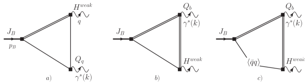
Figure 4: Figures for off-shell form factors $V,T_{\perp,\parallel,{\mathbb{L}}}^{*}$ and $P^{*}$. The single/double lines denote the $q/b$-quark respectively. The diagrams on the left and right are the perturbative- and the one on the left is the quark condensate-type. The quark condensate diagram corresponding to fig a) is not shown. It is proportional to $\langle\bar{q}q\rangle/k^{2}$ and implicitly assumes $k^{2}\neq 0$. In the $k^{2}\to 0$ limit these diagrams are replaced by the photon distribution amplitude e.g. [35]. In the SR method the $B$-meson is projected out via a dispersion relation in the variable $p_{B}^{2}$ giving access to the matrix element of the off-shell form factor $F^{*}(q^{2},k^{2})$. The momentum assignment corresponds to the convention in the Appendix which differs from the phenomenological discussion in the main text.

A.3.2 Explicit results for the off-shell form factors from QCD sum rules

The explicit FFs are found to be

$$P^{*}(0,k^{2}) \;=\; \frac{e^{m_{B_{q}}^{2}/M^{2}}}{f_{B_{q}}m_{B_{q}}^{2}}Q_{b}\left(\,\int_{m_{b}^{2}}^{s_{0}}e^{-s/M^{2}}\rho_{P^{*}}(s,0,k^{2})ds-\frac{2}{\bar{m}_{B_{q}}}\langle\bar{q}q\rangle e^{-m_{b}^{2}/M^{2}}\right)+{\cal O}(\alpha_{s},m_{q})\;,$$ (A.58)

$$T_{\perp}^{*}(0,k^{2}) \;=\; \frac{e^{m_{B_{q}}^{2}/M^{2}}}{f_{B_{q}}m_{B_{q}}^{2}}Q_{b}\left(\,\int_{m_{b}^{2}}^{s_{0}}e^{-s/M^{2}}\rho_{T_{\perp}^{*}}(s,0,k^{2})ds+\left(1-\frac{1}{\bar{k}^{2}}\right)\langle\bar{q}q\rangle e^{-m_{b}^{2}/M^{2}}\right)+{\cal O}(\alpha_{s},m_{q})\;,$$

$$T_{{\mathbb{L}}}^{*}(0,k^{2}) \;=\; \frac{e^{m_{B_{q}}^{2}/M^{2}}}{f_{B_{q}}m_{B_{q}}^{2}}Q_{b}\left(\,\int_{m_{b}^{2}}^{s_{0}}e^{-s/M^{2}}\rho_{T_{\mathbb{L}}^{*}}(s,0,k^{2})ds+\left(1-\frac{1}{\bar{k}^{2}}\right)\langle\bar{q}q\rangle e^{-m_{b}^{2}/M^{2}}\right)+{\cal O}(\alpha_{s},m_{q})\;,$$

$$V_{\perp}^{*}(0,k^{2}) \;=\; \frac{e^{m_{B_{q}}^{2}/M^{2}}}{f_{B_{q}}m_{B_{q}}^{2}}Q_{b}\left(\,\int_{m_{b}^{2}}^{s_{0}}e^{-s/M^{2}}\rho_{V_{\perp}^{*}}(s,0,k^{2})ds+\bar{m}_{B_{q}}\left(1-\frac{1}{\bar{k}^{2}}\right)\langle\bar{q}q\rangle e^{-m_{b}^{2}/M^{2}}\right)+{\cal O}(\alpha_{s},m_{q})\;,$$

$$V_{\parallel}^{*}(0,k^{2}) \;=\; \frac{e^{m_{B_{q}}^{2}/M^{2}}}{f_{B_{q}}m_{B_{q}}^{2}}Q_{b}\left(\,\int_{m_{b}^{2}}^{s_{0}}e^{-s/M^{2}}\tilde{\rho}_{V_{\parallel}^{*}}(s,0,k^{2})ds+\bar{m}_{B_{q}}\left(1+\frac{1}{\bar{k}^{2}}\right)\langle\bar{q}q\rangle e^{-m_{b}^{2}/M^{2}}\right)+{\cal O}(\alpha_{s},m_{q})\;,$$

where $\bar{m}_{B_{q}}\equiv m_{B_{q}}/m_{b}$, $\bar{s}\equiv s/m_{b}^{2}$, $\bar{k}^{2}\equiv k^{2}/m_{b}^{2}$ and the perturbative densities

$$\rho_{i}\equiv\frac{N_{c}m_{b}}{4\pi^{2}(\bar{s}\!-\!\bar{k}^{2})^{3}}\hat{\rho}_{i}\;,$$ (A.59)

are given by

$$\hat{\rho}_{P^{*}}(s,0,k^{2}) \;=\; 2\bar{k}^{2}\bar{m}_{B_{q}}/s\Big{(}\big{(}(\bar{s}-\bar{k}^{2})-1\big{)}\,L_{q}+L_{b}\Big{)}\;,$$

$$\hat{\rho}_{T_{\perp}^{*}}(s,0,k^{2}) \;=\; \big{(}\bar{k}^{4}(1-\bar{s})+2\bar{k}^{2}(\bar{s}-1)-(\bar{s}-1)\bar{s}^{2}\big{)}+\bar{k}^{2}\,L_{q}-\bar{k}^{2}\,L_{b}\;,$$

$$\hat{\rho}_{T_{\mathbb{L}}^{*}}(s,0,k^{2}) \;=\; (\bar{s}-1)(5\bar{k}^{2}-\bar{s})(\bar{s}-\bar{k}^{2})+\big{(}\bar{k}^{2}/(\bar{s}-\bar{k}^{2})(4\bar{k}^{4}+7\ \bar{k}^{2}+(5-4\bar{s})\bar{s})\big{)}\,L_{q}+$$

$$\big{(}\bar{k}^{2}/(\bar{s}-\bar{k}^{2})(\bar{k}^{2}(8\ \bar{s}-7)-\bar{s}(8\bar{s}+5))\big{)}\,L_{b}\;,$$

$$\hat{\rho}_{V_{\perp}^{*}}(s,0,k^{2}) \;=\; \bar{m}_{B_{q}}\{\big{(}\bar{k}^{4}-\bar{k}^{2}(\bar{s}-2)\big{)}\,L_{q}+\big{(}\bar{k}^{2}(\bar{s}-2)-\ \bar{s}^{2}\big{)}\,L_{b}\}\;,$$

$$\hat{\rho}_{V_{\parallel}^{*}}(s,0,k^{2}) \;=\; \bar{m}_{B_{q}}\{2(\bar{k}^{2}/\bar{s}^{2})(\bar{s}-1)(\bar{s}-\bar{k}^{2})^{2}+\big{(}(\bar{k}^{2}/\bar{s})\,(\bar{k}^{4}-2\bar{k}^{2}(\bar{s}-1)+\bar{s}^{2}-2\bar{s}+2)\big{)}\,L_{q}+$$

$$\big{(}(\bar{k}^{4}\bar{s}-2\bar{k}^{2}(\bar{s}^{2}-\bar{s}+1)+(\bar{s}-2)\bar{s}^{2})/s\big{)}\,L_{b}\}\;,$$ (A.60)

and the improvement discussed around (A.57) reads in the case at hand

$$\tilde{\rho}_{V^{*}_{\parallel}}=\left[{\rho}_{V^{*}_{\parallel}}-2\rho_{P^{*}}\right]U(s,k^{2})+2\rho_{P^{*}}\;.$$ (A.61)

Further note that the $1/k^{2}$ factor is of no concern since $P^{*}(0,k^{2})\propto k^{2}$. The logarithms $L_{q}$ and $L_{b}$

$$L_{q}\equiv\ln\left(\frac{\bar{k}^{2}}{\bar{s}\left(1+\bar{k}^{2}-\bar{s}\right)}\right)\;,\quad L_{b}\equiv\ln\left(\bar{s}-\bar{k}^{2}+\frac{\bar{k}^{2}}{\bar{s}}\right)\;,$$ (A.62)

lead to imaginary parts in the FFs for $k^{2}>4m_{q}^{2}=0$ and $k^{2}>4m_{b}^{2}$ respectively. From the viewpoint of the original function these singularities are anomalous thresholds which consist of putting all the propagators on-shell. These expression are consistent with the $B\to V\ell\ell$ weak annihilation computation detailed in appendix of Ref. [31] cf. footnote 3 for further remarks. Note that, there is no singularity at $k^{2}=s$ when expanded properly. The condensate contributions could be written in terms of the densities $\rho_{i}$ as well. The backward substitution $e^{-m_{b}^{2}/M^{2}}\langle\bar{q}q\rangle\to\langle\bar{q}q\rangle\delta(s-m_{b}^{2})$ achieves this task.

A few comments on interpreting the results. The $k^{2}\to 0$ limit is not well-defined for the condensates. In that limit the condensates originating from quark lines attached to the photon are replaced by a photon distribution amplitude which makes the FFs computation more involved. However, the perturbative part remains well-defined in that limit. Hence the latter must contribute positively to the $\{T_{\perp,\parallel}(0,0),\,V_{\perp,\parallel}(0,0)\}$ by convention which can be verified indeed by using $Q_{b}=-1/3$ and sending $\hat{k}^{2}\to 0$. The $q^{2}$ constraints (A.9,A.11) are obeyed exactly by the SRs and are assumed as we do not show $\hat{V}_{\mathbb{L}}(0,k^{2})$ and $T_{\parallel}(0,k^{2})$; they are simply redundant. The constraints at $k^{2}=m_{B_{q}}^{2}$ (A.26) are obeyed for the correlation functions with $k^{2}=p_{B}^{2}$. However they do not hold exactly for the FFs as $p_{B}^{2}\approx m_{B_{q}}^{2}$ within the approximation of the Borel procedure. We have checked that these relations hold to within $2\%$ where for the last one we compare to a value of the FF at $q^{2}=10\mbox{GeV}^{\,2}$. In the fits we have implemented these constraints as they are important to cancels the poles present in the Lorentz structures ${R}_{\parallel}^{\mu\rho}$ and ${R}_{\mathbb{L}}^{\mu\rho}$.

The expressions could be improved by $m_{q}\neq 0$, adding the gluon condensate and radiative corrections. The first two are expected to be rather small effects since $1\gg m_{q}/\Lambda_{\textrm{QCD}}$ and $m_{b}\langle\bar{q}q\rangle\gg\langle G^{2}\rangle$. On the other hand, radiative corrections could be sizeable and would reduce the scale uncertainty considerably. This leads us naturally to the sum rule input and error discussion.

A.3.3 Numerical input to sum rules and rough uncertainty estimates

For a LO computation of the sum rule type discussed here the most important uncertainty will be due to the $b$ quark mass and its associated scheme. Since the sum rule is effectively a ratio of two sum rules,

$$F(0,k^{2})=\frac{[f_{B}F(0,k^{2})]_{\textrm{SR}}}{[f_{B}]_{\textrm{SR}}}\;,\quad F=P,T_{\perp,L}V_{\perp,\parallel}\;,$$ (A.63)

various uncertainties cancel. Some guidance can be taken from the NLO computation of the $B$-meson decay constant. For the latter it is well-known that NLO corrections are moderate in the MS-bar mass-scheme [64, 65] it is therefore advisable to use that scheme anticipating the smallest scale uncertainty. The LO expression are $f_{B_{q}},f_{B_{s}}\approx(222,244)\mbox{MeV}$ with the MS-bar mass $m_{b}=4.18(4)\textrm{GeV}$ [66]. In fact the NLO corrections slightly reduce these values, unlike in other schemes, by less than $10\%$. Hence one can anticipate an uncertainty of that order. The other input are the condensates for which $\langle\bar{q}q\rangle_{\mu=2\textrm{GeV}}=-(0.269(2)\textrm{GeV})^{3}$ (e.g. [66]) is well-known from the Gell-Mann Oakes Renner relation and the strange quark condensate is taken from a lattice computation $\langle\bar{s}s\rangle_{\mu=1\textrm{GeV}}=1.08(16)\langle\bar{q}q\rangle_{\mu=1\textrm{GeV}}$ [67]. The SR specific parameters, the Borel mass and the continuum threshold, are determined by a series of constraints. First and foremost we impose these constraints at Euclidean values $k^{2}<0$ as for positive $k^{2}$ the logarithms can lead to large cancellations and invalidate the prcedure. We then proceed by analytic continuation $k^{2}\to-k^{2}$ to obtain the values for $k^{2}>0$ as found in the results of this paper. This is generally believed to be a reasonable approximation as long as $k^{2}$ is not in a resonance region per se (smooth QCD curves). An example where this works well is $e^{+}e^{-}\to\textrm{hadrons}$ in the region above the broad regions as can be inferred from the $R\propto\sigma(e^{+}e^{-}\to\textrm{hadrons})/\sigma(e^{+}e^{-}\to\mu^{+}\mu^{-})$-plots in [66].

The first constraint comes from the formally exact relation,

$$m_{B_{q}}^{2}=-e^{m_{B_{q}}^{2}/M^{2}}\frac{d}{d(1/M^{2})}e^{-m_{B_{q}}^{2}/M^{2}}\ln P^{*}(k^{2},M^{2},s_{0})\,,$$ (A.64)

often referred to as the daughter sum rule, which we require to be satisfied within ${\cal O}(2\%)$. Next $s_{0}$ ought to be in the window $(m_{B}+2m_{\pi})^{2}$ and $(m_{B}+m_{\rho})^{2}$ which is compatible with (A.64). The Borel parameter is further constrained by requiring two standard criteria i) the condensate not to exceed $10\%$ assuring convergence of the OPE ii) the continuum contribution not exceed $30\%$ which assures that the $B$-meson is projected out rather than an entire set of states. Note that the later two conditions are exclusive in that the former requires a large and the latter a smaller Borel parameter. The values adapted for the thresholds are $(s_{0}^{B_{q}},s_{0}^{B_{s}})=(35(2),35.5(2.0))\mbox{GeV}^{2}$. The $B_{d}$ Borel parameter for $P,T_{\perp,L},V_{\perp}$ is taken to be $M^{2}=9(2)\mbox{GeV}^{2}$ for $|k^{2}|<10\mbox{GeV}^{2}$ and $M^{2}=7(2)\mbox{GeV}^{2}$ for $|k^{2}|>15\mbox{GeV}^{2}$ with smooth interpolation and finally $M^{2}_{V_{\parallel}}=6(2)\mbox{GeV}^{2}$. A global shift is applied for the $B_{s}$ Borel parameters $M^{2}_{B_{s}}=M^{2}_{B_{q}}+0.5\mbox{GeV}^{2}$, which respect the mass ratios of the meson roughly.

Let us turn to the uncertainty analysis. For the main section we use a $z$-expansion fit with similar uncertainty analysis as in Ref. [29] with some more detail delegated to the fit-section. This analysis and fit is restricted to high $q^{2}$. In addition we append a Mathematica notebook to the arXiv version for reproducing the plots. The brief comments on uncertainties apply to this version. The main sources of uncertainty are the Borel parameter and the scale uncertainty. The threshold uncertainty is negligible and the quark condensate uncertainty is only relevant for the $B_{s}$-mode where its impact is still moderate in almost all cases and regions. The uncertainty due to NLO corrections is estimated to be $15\%$ on grounds of the known radiative corrections to the $B$-meson decay constant as previously discussed in this section. The uncertainty of the Borel parameter is roughy $20\%$, which is on the conservative side, and when added in quadrature this amounts to a $\approx 25\%$ uncertainty. An NLO computation would presumably not only reduce the scale but also the Borel uncertainty. We refrain from a more elaborate error analysis altogether including the extension in the resonance region. This is in principle not difficult to achieve in that one can at first just vary the input into the dispersion relation. This procedure ought to give a reasonable error estimate.

A.4 Extending the off-shell form factors below the ${\cal O}(2\mbox{GeV}^{\,2})$-region

The QCD SR results (A.58) of the last section are valid for $k^{2}>{\cal O}(2\mbox{GeV}^{\,2})$. They are not valid below, since the low-lying vector meson resonances such as the $\phi$-meson, in the $B_{s}$-case, distort the amplitude considerably. Conversely the $1/k^{2}$-factors of the condensates, which mimic these effects in the region of validity become singular in this limit. On the other hand a fair amount is known on the FFs in that region, as previously discussed, cf. appendix A.2 and (A.2) in particular, including the on-shell $B\to\gamma$ FFs and the $B_{s}\to\phi$ FFs. We advocate that optimal use of this knowledge can be made by using a multiple subtracted dispersion relation with input of this hadronic data and the use of the OPE from the QCD SR for sufficiently large $k^{2}$. This is illustrated in Figure 5.

We first begin by discussing the dispersion relation. We write the generic FF, denoted by $F$, as the sum of subtraction terms and the dispersion integral

$$F(k^{2})=F_{12}^{\textrm{sub}}(k^{2})+F^{\textrm{dis}}_{12}(k^{2})$$ (A.65)

where the subscript $``12"$ refers to a single subtraction point at $k_{0}^{2}$ and a double subtraction point at $k_{1}^{2}$. The double subtraction ensures that even the derivatives is continous at the matching point. The subtraction term is given by

$$F_{12}^{\textrm{sub}}(k^{2})=U(k^{2},k_{1}^{2},k_{0}^{2})^{2}F(k_{0}^{2})+U(k^{2},k_{0}^{2},k_{1}^{2})\big{(}\frac{k_{0}^{2}-2k_{1}^{2}+k^{2}}{k_{0}^{2}-k_{1}^{2}}F(k_{1}^{2})+(k^{2}-k_{1}^{2})F^{\prime}(k_{1}^{2})\big{)}\;,$$ (A.66)

where the prime denotes the derivative, $U(a,b,c)\equiv\frac{a-b}{c-b}$, and the dispersion integral reads

$$F^{\textrm{dis}}_{12}(k^{2})=\frac{1}{\pi}\int^{\infty}_{\textrm{cut}}\frac{du\,\textrm{Im}[F(u)]}{u-k^{2}-i0}w_{12}(k^{2},u)\;,\quad w_{12}(k^{2},u)=U(k^{2},k_{0}^{2},u)U(k^{2},k_{1}^{2},u)^{2}\;,$$ (A.67)

where it was used that $F$ is real somewhere on the real axis so that Schwartz’s reflection principle applies. We emphasise that these expressions are exact as it is in essence based on partial fraction decomposition.

Let us turn to the specific treatment proposed. The first step is to write, in close analogy with (A.2),

$$F^{\textrm{dis}}_{12}(k^{2})\to F^{\textrm{dis-QHD}}_{12}(k^{2})=\frac{r^{\phi}_{F}}{m_{\phi}^{2}-k^{2}-im_{\phi}\Gamma_{\phi}}w_{12}(k^{2},m_{\phi}^{2})+\frac{1}{\pi}\int^{\infty}_{u_{0}}\frac{du\,\textrm{Im}F^{\textrm{PT}}(u)}{u-k^{2}-i0}w_{12}(k^{2},u)\;,$$ (A.68)

where the the acronym QHD stands for quark-hadron duality in the sense of semi-global quark-hadron duality, used in QCD SR,

$$\int^{\infty}_{\textrm{cut}}\frac{du\,\textrm{Im}F(u)}{u-k^{2}-i0}w_{12}(k^{2},u)\approx\int^{\infty}_{u_{0}}\frac{du\,\textrm{Im}F^{\textrm{PT}}(u)}{u-k^{2}-i0}w_{12}(k^{2},u)\;,$$ (A.69)

with the difference that there is no Borel transformation but subtraction terms instead. The superscript PT stands for perturbation theory whereby we mean the SR computation where the condensates are dropped. The quantity $u_{0}$ is an effective threshold marking the onset of multiple particle states and the $\phi(1680)$-meson (and the $\rho^{\prime}/\omega^{\prime}$ etc in the $B_{d}$-case). The residue $r^{\phi}_{F}$ is specific to the FF and can be inferred from the equations in appendix A.2. Finally we can make the outline sketched at the beginning of the section concrete

$$F(k^{2})=\left\{\begin{array}[]{ll}F^{\textrm{hdis}}(k^{2})&0<k^{2}<k_{1}^{2}\\[14.22636pt] F^{\textrm{OPE}}(k^{2})&k_{1}^{2}<k^{2}\ll 4m_{b}^{2}\end{array}\right.\;,$$ (A.70)

where $F^{\textrm{hdis}}(k^{2})\equiv F_{12}^{\textrm{sub}}(k^{2})+F_{12}^{\textrm{dis-QHD}}(k^{2})$, and the acronym “hdis” stands for hadronic dispersion relation (which is the correct approach when used in the region of discontinuities), and the OPE superscript corresponds to the QCD-SR expressions found in (A.58) which is based on the perturbative and the condensate contributions. In the following we refer to (A.70) as the improved FF.

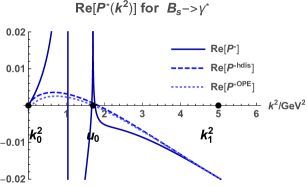
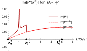
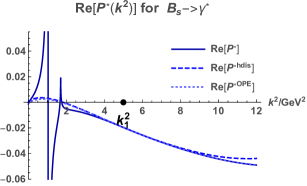
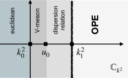
Figure 5: At the top left and right we plot the $P^{*}(k^{2})$ FF as an example in the region between the first and the second subtraction point $k_{0}^{2}=0\mbox{GeV}^{\,2}$ and $k_{1}^{2}=5\mbox{GeV}^{\,2}$ for the improved FF ($P^{*}$), the subtracted dispersion relation ($P_{12}^{*\textrm{dis}}$) and the QCD-SR version ($P^{*\textrm{OPE}}$). As expected the QCD-SR version, which is based on the asymptotically valid OPE, does not satisfy the constraint $P^{*}(0)=0$. Other than at this point the QCD-SR and the dispersion relation version are rather similar where the improved version is very different of course because of the inclusion of $\phi$-meson. On the bottom part we show the matching region on the left and a plot showing how the dispersion relation differs from the QCD-SR version for $k^{2}\gg 5\mbox{GeV}^{\,2}$ which is again expected since the polynomial nature of the subtraction points will invalidate its use as well as the on-set of the condensate terms. On the right we show the imaginary part where by construction $\textrm{Im}(P^{*\textrm{OPE}})=\textrm{Im}(P_{12}^{*\textrm{dis}})$ and the improved version is identical above the second matching point.

A.4.1 Some detail on the double dispersion relation including the numerical input

So far we have been somewhat formal on how to obtain the concrete dispersion relations within our specific computation. We first give the recipe for the explicit integrals before stating the sources of numerical input.

We may parameterise the densities in (A.58) as follows $\rho_{F}=-q_{F}L_{q}-b_{F}L_{b}+\textrm{rest}$, and then its discontinuity $\rho_{D}$, which is formally a double discontinuity, is defined and given by

$$\rho^{D}_{F}(s,u) \;=\; \frac{1}{2\pi i}\big{(}\rho(s,0,u+i0)-\rho(s,0,u-i0)\big{)}$$ (A.71)

$$\;=\; q_{F}\big{(}\Theta(u)-\Theta[u-(s-m_{b}^{2})]+b_{F}\Theta[u-s^{2}/(s-m_{b}^{2})\big{)}\;,$$

where $q^{2}=0$ is not shown explicitly for brevity. The subscript $q$ and $b$ indicate whether the photon is emitted from a $q=d,s$ or a $b$ quark. The purely dispersive $F^{\textrm{dis}}_{12}$ (A.67) reads

$$F^{\textrm{dis}}_{12}(k^{2}) \;=\; p\int_{0}^{\infty}\frac{du}{u-k^{2}-i0}\int_{u+m_{b}^{2}}^{s_{0}}dse^{-\frac{s}{M^{2}}}\rho^{D}_{F}(s,u)w_{12}(k^{2}+i0,u)$$ (A.72)

$$\;=\; p\int_{m_{b}^{2}}^{s_{0}}dse^{-\frac{s}{M^{2}}}\left(\int_{0}^{s-m_{b}^{2}}\!\!\!\frac{du\,w_{12}(k^{2}+i0,u)}{u-k^{2}-i0}q_{F}(s,u)+\int_{\frac{s^{2}}{s-m_{b}^{2}}}^{\infty}\!\!\!\frac{du\,w_{12}(k^{2}+i0,u)}{u-k^{2}-i0}b_{F}(s,u)\right)\;,$$

where $p\equiv\frac{e^{m_{B_{q}}^{2}/M^{2}}}{f_{B_{q}}m_{B_{q}}^{2}}Q_{b}$ is a common prefactor. We have verified numerically that these relations work for all five off-shell FFs. The improved version in the resonance region is then given by

$$F^{\textrm{hdis}}(k^{2})=F_{12}^{\textrm{sub}}(k^{2})+F^{\textrm{dis}}_{12}(k^{2})+[\delta F_{12}(k^{2})]_{u_{0}}$$ (A.73)

with the improvement term

$$[\delta F_{12}(k^{2})]_{u_{0}}=\frac{r^{\phi}_{F}}{m_{\phi}^{2}-k^{2}-im_{\phi}\Gamma_{\phi}}w_{12}(k^{2},m_{\phi}^{2})-[F^{\textrm{dis}}_{12}]_{u_{0}}(k^{2})\;,$$ (A.74)

where

$$[F^{\textrm{dis}}_{12}]_{u_{0}}(k^{2}) \;=\; p\int_{0}^{u_{0}}\frac{du}{u-k^{2}}\int_{u+m_{b}^{2}}^{s_{0}}dse^{-\frac{s}{M^{2}}}\rho^{D}_{F}(s,u)=p\int_{m_{b}^{2}}^{s_{0}}dse^{-\frac{s}{M^{2}}}\!\!\!\!\!\!\!\!\!\!\!\!\int_{0}^{\textrm{min}(u_{0},s-m_{b}^{2})}\!\!\!\!\!\!\!\!\!\frac{du\,w_{12}(k^{2},u)}{u-k^{2}}q_{F}(s,u)\;,$$ (A.75)

where the emission from the $b$-quark has not support in the $[0,u_{0}]$ interval since the cut only starts at $4m_{b}^{2}\gg u_{0}$. This completes the formal recipe. However, for the numerical implementation, replacing (A.73) by the following expression

$$F^{\textrm{hdis}}(k^{2})\;=\;\delta F_{12}^{\textrm{sub}}(k^{2})+F^{\textrm{PT}}(k^{2})+[\delta F_{12}(k^{2})]_{u_{0}}\;,$$ (A.76)

is even better suited as it avoids an integral to infinity. Above $F^{\textrm{PT}}$ is the SR expression without condensates, $[\delta F_{12}]_{u_{0}}$ as in (A.74) and $\delta F_{12}^{\textrm{sub}}$ is given by

$$\delta F_{12}^{\textrm{sub}}(k^{2})=F_{12}^{\textrm{sub}}(k^{2})\big{|}^{F(k_{1}^{2})\to F^{\bar{q}q}(k_{1}^{2})}_{F(k_{0}^{2})\to F^{B\to\gamma}(k_{0}^{2})-F_{\textrm{PT}}(k_{0}^{2})}\;,$$ (A.77)

with $F_{12}^{\textrm{sub}}$ given in (A.66). The expression (A.76), which is formally equivalent to the former one, make the continuity of the matching condition up to the first derivative manifest,

$$F^{\textrm{hdis}}(k_{1}^{2}) \;=\; F^{\textrm{PT}}(k_{1}^{2})+F^{\bar{q}q}(k_{1}^{2})=F^{\textrm{OPE}}(k_{1}^{2})\;,$$

$$F^{{}^{\prime}\textrm{hdis}}(k_{1}^{2}) \;=\; F^{{}^{\prime}\textrm{PT}}(k_{1}^{2})+F^{{}^{\prime}\bar{q}q}(k_{1}^{2})=F^{{}^{\prime}\textrm{OPE}}(k_{1}^{2})\;.$$ (A.78)

Above we used $[\delta F_{12}(k_{1}^{2})]_{u_{0}}=0$ and the prime denotes again the derivative.

The improved version is absolutely necessary when considering a decay rate as then the resonance, cf. Figure 5, is effectively squared and one will otherwise not get a correct expression. There is no quark-hadron duality at the level of exclusive decay rates! However, quark-hadron duality applies at the level of amplitudes since they obey dispersion relations. One can therefore evaluate them away from the resonance region. Within the resonance region, a reasonable approximation is obtained when averaged over a sufficiently large interval that does not end in a resonance region. Thus averaging the FF over $[0,k_{1}^{2}]$ in $dk^{2}$ should provide reasonable agreement between the QCD-SR and improved FF. Indeed we find that in all cases this average well within a factor of two. This is remarkable when one inspects the shapes and considers the uncertainties of all the numerical input per se. We stress that it is the improved FF that is expected to give the reliable average and the difference to the QCD-SR result is another reason for introducing the improved FF.

We now turn to the required numerical input. For $F_{12}^{\textrm{sub}}(k^{2})$ we just need the matching points. For the first subtraction point we choose $k_{0}^{2}=0$ since the FFs are known at this point from $B\to\gamma$ at zero momentum transfer in the weak matrix element. For the five FFs at hand they are given by

$$P^{*}(0,0)=0\;,\quad T^{*}_{\perp}(0,0)=T_{\mathbb{L}}(0,0)=T_{\perp}^{B\to\gamma}(0)\;,\quad V_{\perp,\parallel}^{*}(0,0)=V^{B\to\gamma}_{\perp,\parallel}(0)\;,$$ (A.79)

where concretely $T_{\perp}^{B_{(d,s)}\to\gamma}(0)=(0.130(13),0.160(15))$, $V^{B_{(d,s)}\to\gamma}_{\perp}(0)=(0.079(9),0.105(8))$ and $V^{B_{(d,s)}\to\gamma}_{\parallel}(0)=(0.129(13),0.153(14))$ [35] are used. The second matching point is taken at $k_{1}^{2}=5\mbox{GeV}^{\,2}$ which is far enough above $u_{0}=1.7(2)\mbox{GeV}^{\,2}$ for the $B_{s}$-case ($u_{0}=1.5(2)\mbox{GeV}^{\,2}$ for the $B_{d}$-case) as well as high enough to trust the OPE even when analytically continued to Minkowski space.

The term $F^{\textrm{dis-QHD}}_{12}(k^{2})$ in (A.68) consists of the pole term and the dispersion integral. The data entering the pole part is, of course, the same as in (A.2) and consists of the pole data: masses and decay widths as well as the residue which is a product of the decay constant and the $B\to\phi[\rho,\omega]$ FFs at zero momentum transfer. The former are determined in large from experiment and taken from the analysis in appendix C in [29]. The FFs are taken from the same reference which consists of a NLO LCSR analysis.

A.4.2 Plots of the off-shell form factors

Plots of the five FFs are shown in Figure 6 in the non-resonant region and three examples in the resonant region. Whereas all of these FFs asymptotically tend to a constant due to the condensate term, as discussed in footnote 14, $T^{*}_{\perp,L}$ and $V_{\perp}$ tend towards zero since there is a cancellation for $k^{2}\approx m_{b}^{2}$. The imaginary part drops to zero at around $k^{2}=s_{0}-m_{b}^{2}$ as can be inferred from (A.71). Both effects will presumably be lifted at NLO. The partonic computation acquires an imaginary part at $k^{2}>4m_{b}^{2}$ which is however far to the left of the plot-window and thus not visible. In the hadronic region the single resonance is used together with a continuum threshold. The later results in a $\ln(u_{0}-k^{2})$ and is representative of two particle thresholds and effects from higher resonances and the $\phi^{\prime}$. Obviously in the vicinity of $u_{0}$ the result is to be used in the sense of bins only.

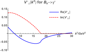
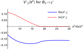
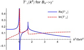
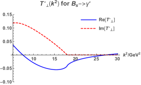
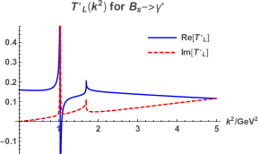
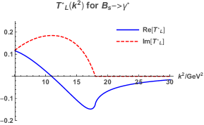
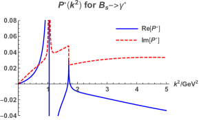
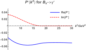
Figure 6: Plots of the five FFs in the OPE region $[5,30]\mbox{GeV}^{\,2}$ with formulae in (A.58) and denoted by $F^{\textrm{OPE}}$. In three cases (the $V_{\perp,\parallel}$ case are similar to $T_{\perp,L}$ in that region) we plot the $[0,5]\mbox{GeV}^{\,2}$-region where the vector meson resonance is visible. For $P^{*}$ the reader can find more plots in Figure 5.

A.5 Dispersion relation and fit ansatz for form factors

A.5.1 Extending the $B\to\gamma$ on-shell form factors into the $q^{2}\approx m_{B}^{2}$-region

The $B\to\gamma$ on-shell FFs $F(q^{2})\equiv F^{*}(q^{2},0)$, cf. (A.1.3), taken from the NLO LCSR analysis [35]. The region of validity of the computation is the previously mentioned $q^{2}<m_{b}\Lambda$ which is just outside our region of interest $q^{2}\in[(4.9\mbox{GeV})^{2},m_{B_{d,s}}^{2}]$. Progress can be made with the help of the generally valid dispersion representation in the flavour-violating momentum transfer $q^{2}$

$$V_{\perp}(q^{2}) \;=\; \frac{1}{\pi}\int_{\textrm{cut}}^{\infty}\frac{\textrm{Im}[V_{\perp}(t)]\,dt}{t-q^{2}-i0}=\frac{r_{V_{\perp}}}{1-q^{2}/m_{B^{*}_{q}}^{2}}+\dots\;,$$

$$V_{\parallel}(q^{2}) \;=\; \frac{1}{\pi}\int_{\textrm{cut}}^{\infty}\frac{\textrm{Im}[V_{\parallel}(t)]\,dt}{t-q^{2}-i0}=\frac{r_{V_{\parallel}}}{1-q^{2}/m_{B_{q1}}^{2}}+\dots\;,$$ (A.80)

where the dots stand for higher resonances and multiparticle states. The values and quantum numbers of the resonances are collected in Table 7. The dispersion relations of the other FFs are analogous. The residua are related to the $B_{q}^{*}\to B_{q}\gamma$ and $B_{q1}\to B_{q}\gamma$ on-shell matrix elements respectively. Unfortunately they are not known from experiment. They can be extracted from the same SR as the FFs themselves by applying a double dispersion relation to interpolate for the $B_{q}^{*}$- and $B_{q1}$-meson respectively. We take the NLO result of this residue from [36], collected in Table 6.

$$\begin{array}[]{ l r r r r }&r_{V_{\perp}}\propto g_{B_{q}^{*}B_{q}\gamma}&r_{T_{\perp}}\propto g_{B_{q}^{*}B_{q}\gamma}&r_{V_{\parallel}}\propto g_{B_{q1}B_{q}\gamma}&r_{T_{\parallel}}\propto g_{B_{q1}B_{q}\gamma}\\ \hline\cr\hline\cr B_{d}\to\gamma&\phantom{-}0.179^{+0.019}_{-0.019}&0.171^{+0.018}_{-0.020}&0.076^{+0.015}_{-0.016}&0.104^{+0.015}_{-0.015}\\[2.84544pt] B_{s}\to\gamma&\phantom{-}0.235^{+0.024}_{-0.025}&0.224^{+0.023}_{-0.024}&0.114^{+0.016}_{-0.018}&0.146^{+0.017}_{-0.017}\\ \hline\cr\end{array}$$

Table 6: The residua of the poles at $k^{2}=m_{B_{q}^{*}}^{2},m_{B_{q1}}^{2}$ proportional to the on-shell matrix of an NLO computation [36].

Here, we make the link to the predictions of Ref. [41], for which a single $m_{B_{s}^{*}}$-pole approximation was employed to estimate the FFs for the radiative decay. The single-pole approximation is expected to give a reasonable approximation around the pole provided the residue is known sufficiently well. By identifying the defining matrix elements of the residue (cf. Eq.(6) in Ref. [41]) we find the relation

$$|r_{V_{\perp}^{B_{s}\to\gamma}}|=|\mu|f_{B_{s}}|_{\mbox{\cite[cite]{[\@@bibref{Number}{Aditya:2012im}{}{}]}}}\approx 0.265\;,$$ (A.81)

with $f_{B_{s}}=227\textrm{MeV}$ [66] the standard decay constant and $|\mu|$ defines the strength of the on-shell matrix element in Ref. [41]. The authors of Ref. [41] determine $|\mu|=1.13\,\mbox{GeV}^{\,-1}$ in an effective-theory approach valid at leading order in $1/m_{b,c}$ using experimental data from $D^{*+}\to D^{+}\gamma$ and $D^{*0}\to D^{+}\pi^{-}$. They neglect the pole of the $B_{s1}$ meson (cf. Table 7) and thus we cannot compare the $|r_{V_{\parallel}}|$ residua to theirs. Given the methods employed on both sides the agreement of $0.235(23)$ and $0.265$ is presumably somewhat accidental. Whereas the former is LO in the coupling with preliminary error analysis, the latter is subject to $1/m_{c}$ corrections which might well be sizeable.

At last let us mention that we performed a non-trivial test of the identification in Eq. (A.81). Approximating our FF-expression to the pole part, inserting it into our rate in Eq. (2.15), and then comparing to the rate in Ref. [41] (cf. their Eq. (25)), we can confirm that Eq. (A.81) is consistent with both rates. This is a strong hint of the correctness of the treatment in our work and theirs.

A.5.2 The dispersion representation of the $B\to\gamma^{*}$ off-shell form factors

The assumed $q^{2}=0$ is well below the various $m_{B}^{2}$-type poles and does not affect the computation. However, in the variable $k^{2}$ there are the previously mentioned $\rho/\omega$ ($\phi$)- and $\Upsilon$-resonances (cf. Table 7) which are far away from our region of interest $k^{2}\approx m_{B}^{2}$ and therefore have little impact. If one wanted to fit the FFs at lower $k^{2}$ then a dispersion ansatz, e.g. (A.2), could be combined with the $z$-expansion.

$$\begin{array}[]{ l rrr }&m_{B_{q}}=m_{0^{-}}&m_{B^{*}}=m_{1^{-}}=m_{\perp}&m_{B_{q1}}=m_{1^{+}}=m_{\parallel}\\ \hline\cr\hline\cr{b\to s}&5.367\,\textrm{GeV}&5.415\,\textrm{GeV}&5.829\,\textrm{GeV}\\ {b\to d,u}&5.280\,\textrm{GeV}&5.325\,\textrm{GeV}&5.726\,\textrm{GeV}\\ \hline\cr\end{array}$$

Table 7: Lowest resonance masses for FFs [66]. The mass $m_{0^{-}}$ is the $B$-meson mass in $B_{q}\to\gamma$. The Form Factors $V,T_{\perp}$ and $V,T_{\parallel}$ are associated with the resonances $J^{P}=1^{-}$ and $1^{+}$ respectively.

A.5.3 Fit ansatz and $z$-expansion

The procedure to fit the FFs and how to include the correlation of uncertainties largely follows Ref. [29]. Based on the previous part of this section let us first motivate the fit-ansatz before summarising the essence of the $z$-expansion. There are four on-shell FFs and at $q^{2}=0$ there are five off-shell FFs,

on-shell: $$\{V^{B\to\gamma}_{\perp,\parallel}(q^{2}),T^{B\to\gamma}_{\perp,\parallel}(q^{2})\}\;,$$

off-shell: $$\{P^{B\to\gamma^{*}}(0,k^{2})\;,V^{B\to\gamma^{*}}_{\perp,\parallel}(0,k^{2}),\;T^{B\to\gamma^{*}}_{\perp,{\mathbb{L}}}(0,k^{2})\}\;.$$ (A.82)

• The on-shell FFs are parameterised

  $$F_{n}^{B\to\gamma}(q^{2})=\frac{1}{1-q^{2}/m_{R}^{2}}\left(\alpha_{n0}+\sum_{k=1}^{N}\alpha_{nk}(z(q^{2})-z(0))^{k}\right)\;,$$ (A.83)

  using the knowledge of the presence of the first pole $m_{R}$ (A.5.1), cf., Table 7. The remaining part in brackets are supposed to take into account higher states in the spectrum. Specifically the $\alpha_{nk}$-coefficients are to be determined from a fit and $z(q^{2})$ is defined further below. The constraint of the residue, cf. (A.5.1) and Table 6, is implemented by

  $$r_{V_{\perp}}=\alpha_{V_{\perp}0}+\sum_{k=1}^{N}\alpha_{V_{\perp}k}(z(m_{B^{*}_{q}}^{2})-z(0))^{k}\;,$$ (A.84)

  and similarly for other FFs. Further to that the constraint (A.11) is imposed by

  $$T^{B\to\gamma}_{\perp}(0)=T^{B\to\gamma}_{\parallel}(0)\;\;\Leftrightarrow\;\;\alpha_{T_{\perp}0}=\alpha_{T_{\parallel}0}\;.$$ (A.85)

• The off-shell FFs are simply parameterised by

  $$F_{n}^{B\to\gamma^{*}}(0,k^{2})=\alpha_{n0}+\sum_{k=1}^{N}\alpha_{nk}(z(k^{2})-z(0))^{k}\;,$$ (A.86)

  The constraint $V_{\parallel}^{*}(0,m_{B_{q}}^{2})=2P^{*}(0,m_{B_{q}}^{2})$ (A.26) is imposed

  $$\alpha_{V_{\parallel}^{*}0}+\sum_{k=1}^{N}\alpha_{V_{\parallel}^{*}k}(z(m_{B^{*}_{q}}^{2})-z(0))^{k}=2\big{(}\alpha_{P^{*}0}+\sum_{k=1}^{N}\alpha_{p^{*}k}(z(m_{B^{*}_{q}}^{2})-z(0))^{k}\big{)}\;.$$ (A.87)

  The fit-ansatz (A.86) could easily be improved including the information on the $\rho/\omega$ ($\phi$)-like resonances from the dispersion representation (A.2).

Let us now describe the $z$-expansion in order to remain self-consistent. The function $z(t)$ is defined by

$$z(t)=\frac{\sqrt{t_{+}-t}-\sqrt{t_{+}-t_{0}}}{\sqrt{t_{+}-t}+\sqrt{t_{+}-t_{0}}}\;,$$ (A.88)

where $t_{0}\equiv t_{+}(1-\sqrt{1-t_{-}/t_{+}})$ and $t_{\pm}\equiv(m_{B_{q}}\pm m_{\rho})^{2}$. The $\rho$-mass, $m_{\rho}=770\mbox{MeV}$, is just an arbitrary reference scale and the values of $m_{B_{q}}$ are given in Table 7.

The coefficients $\alpha_{nk}$ are determined by fitting $N=200$ random points at each integer value of $q_{i}^{2}$ (in $\textrm{GeV}^{2}$-units) in a specific interval. Uncertainties in input parameters, $p\pm\delta p$, as for example $m_{b}$, are accounted for by sampling them with a normal distribution $N(p,\delta p)$, which accounts for the same correlations as in Ref. [29]. The $N=200$ random samples of $F_{I}=F_{i}(q_{j}^{2})$, where $I=(i,j)$ denotes the collective index for the FF-type and the momentum, determine the $(ij)\times(ij)$ covariance matrix

$$C_{IJ}=\langle F_{I}F_{J}\rangle-\langle F_{I}\rangle\langle F_{J}\rangle\,.$$ (A.89)

Angle brackets denote the average over random samples. The coefficients $\alpha_{nk}$ are then found by minimising the function

$$\chi^{2}(\{\alpha\})=\sum_{IJ}(F_{I}^{\text{sample}}-F_{I}^{\text{fit}}(\{\alpha\}))C_{IJ}^{-1}(F_{J}^{\text{sample}}-F_{J}^{\text{fit}}(\{\alpha\}))\;,$$ (A.90)

for each random sample, where the correlation matrix remains constant for all samples. The fitted values of $\alpha$ are then averaged over all the samples and errors are calculated from the standard deviation, which is justified because each of the samples are statistically independent.

• The computation of the four on-shell FFs [35] are limited to roughly $q^{2}<14\mbox{GeV}^{\,2}$. The $200$ sample points are generated for each integer interval in $q^{2}\in[-5,14]\mbox{GeV}^{\,2}$ to which the $\alpha_{n}$’s are then fitted to the ansatz (A.86).

• Since we only need the off-shell FFs in the region $k^{2}\in[(4.9\mbox{GeV})^{2},m_{B_{d,s}}^{2}]\mbox{GeV}^{\,2}$ we restrict our fitting procedure to this region.

Appendix B The $B_{q}\to\ell\ell\mathbb{V}$ for searches beyond the Standard Model

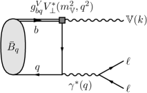
Figure 7: Illustration of the three-body decay of a $B_{q}$ to a pair of leptons and a new, light, beyond-the-standard-model vector $\mathbb{V}$ induced by a flavour-violating vector coupling ($\bar{b}\not{\mathbb{V}}q$, see Lagrangian in Eq. (B.1)).

The main focus of this work has been to propose a search for the QCD axion via the three-body decay $B_{q}\to\ell\ell a$ and the computation of the FFs contributing to this beyond-the-SM decay channel as well as to the radiative $B_{q}\to\ell\ell\gamma$ decay. However, the computation of the off-shell FFs allows us to extend this analysis to searches for light, beyond-the-SM vector bosons ($\mathbb{V}$) with flavour violating couplings. In this appendix, we present the $B_{q}\to\ell\ell\mathbb{V}$ rate, which is relevant for a search via $B_{q}\to\mu\mu$, and briefly discuss the search’s sensitivity.

We parametrise the relevant flavour violating couplings via the effective Lagrangian

$$\mathscr{L}_{\mathbb{V}} =\left(\mathbb{V}_{\mu}\bar{q}\gamma^{\mu}\left(g^{V}_{bq}\frac{m_{\mathbb{V}}^{2}}{\Lambda^{2}}+g^{A}_{bq}\frac{m_{\mathbb{V}}^{2}}{\Lambda^{2}}\gamma_{5}\right)b+\partial_{\mu}\mathbb{V}_{\nu}\bar{q}\sigma^{\mu\nu}\left(\frac{g_{bq}^{T}}{\Lambda}+\frac{g_{bq}^{T_{5}}}{\Lambda}\gamma_{5}\right)b+\text{h.c.}\right)-\frac{1}{2}m_{\mathbb{V}}^{2}\mathbb{V}^{\mu}\mathbb{V}_{\mu}\;,$$ (B.1)

where $\Lambda$ is the heavy NP scale. Above, we opted to factorise out the term $m_{\mathbb{V}}^{2}/\Lambda^{2}$ in the dimension-four vector- and axial-vector couplings to demonstrate the “restoration” of gauge invariance in the limit $m_{\mathbb{V}}\to 0$. We further introduce the quantities

$$\hat{g}_{bq}^{V}\equiv\frac{m_{\mathbb{V}}^{2}}{\Lambda^{2}}g_{bq}^{V}\,, \hat{g}_{bq}^{A}\equiv\frac{m_{\mathbb{V}}^{2}}{\Lambda^{2}}g_{bq}^{A}\,, \hat{g}_{bq}^{T}\equiv\frac{m_{B_{q}}}{\Lambda}g_{bq}^{T}\,, \hat{g}_{bq}^{T_{5}}\equiv\frac{m_{B_{q}}}{\Lambda}g_{bq}^{T_{5}}\,.$$ (B.2)

which simplify some of the intermediate formulae.

Based on Eq. (B.1) we compute the $B_{q}\to\ell\ell\mathbb{V}$ rate using the helicity formalism. The $B_{q}\to\ell\ell\mathbb{V}$ decay differs from the semileptonic and flavour-changing-neutral-current decays $B\to\rho\ell\nu$ and $B\to K^{*}\ell\ell$ in that the vector meson is emitted from the weak vertex and the lepton pair originates from an off-shell photon cf. Figure 7. The helicity amplitude for the decay reads

$${\cal A}_{\lambda}\propto\omega^{*}_{\mu}(\mathbb{V},k,\lambda)\epsilon_{\rho}^{*}(\gamma^{*},q,\lambda)~{}\left(\hat{g}^{V}_{bq}M^{\rho\mu}_{V}+\hat{g}^{A}_{bq}M^{\rho\mu}_{A}+\hat{g}^{T}_{bq}M^{\rho\mu}_{T}+\hat{g}^{T_{5}}_{bq}M^{\rho\mu}_{T_{5}}\right)$$ (B.3)

where $g^{T}_{bq}\equiv m_{B_{q}}/\Lambda^{T}_{bq}$ and analogous for $T_{5}$ as this leads to transparent formulae. Explicit polarisation vectors are given in Eq. (A.1.3). The helicity amplitudes are then given by

$$\begin{split}{\cal A}_{\perp}&\;=\;(\lambda^{(\mathbb{V})}_{B_{q}})^{1/2}F_{\perp}\;,\\[2.84544pt] {\cal A}_{\parallel}&\;=\;(m_{\mathbb{V}}^{2}-m_{B_{q}}^{2})F_{\parallel}\;,\\[2.84544pt] {\cal A}_{0}&\;=\;\frac{m_{\mathbb{V}}}{2\sqrt{2q^{2}}(m_{B_{q}}^{2}-q^{2})}\left(\lambda^{(\mathbb{V})}_{B_{q}}F_{\mathbb{L}}-(m_{B_{q}}^{2}-m_{\mathbb{V}}^{2})(m_{B_{q}}^{2}-m_{\mathbb{V}}^{2}+3q^{2})F_{\parallel}\right)\;,\end{split}$$ (B.4)

with $\lambda^{(\mathbb{V})}_{B_{q}}=\lambda(m_{B}^{2},q^{2},m_{\mathbb{V}}^{2})$ and the FFs

$$F_{\perp}=\hat{g}^{V}_{bq}V^{*}_{\perp}(m_{\mathbb{V}}^{2},q^{2})+\hat{g}^{T}_{bq}T^{*}_{\perp}(m_{\mathbb{V}}^{2},q^{2})\;,\quad F_{\parallel,\mathbb{L}}=\hat{g}^{A}_{bq}V^{*}_{\parallel,\mathbb{L}}(m_{\mathbb{V}}^{2},q^{2})-\hat{g}^{T_{5}}_{bq}T^{*}_{\parallel,\mathbb{L}}(m_{\mathbb{V}}^{2},q^{2})\;.$$ (B.5)

The minus sign in the last expression originates from the minus sign in Eq. (2.1).

Our FFs provide a good description in the case where $m_{\mathbb{V}}$ is much smaller than all other scales since we have evaluated them for $m_{\mathbb{V}}=0$. Three observations on the helicity amplitudes are in order. Firstly, in the $m_{\mathbb{V}}\to 0$ limit the pseudoscalar part in the longitudinal component survives since $V_{\mathbb{L}}^{*}(m_{\mathbb{V}}^{2},q^{2})=-2m_{B_{q}}^{2}/m_{\mathbb{V}}^{2}\hat{V}^{*}(m_{\mathbb{V}}^{2},q^{2})$ in general and $\hat{V}^{*}(0,q^{2})=P^{*}(0,q^{2})$ in particular. Secondly, in the $m_{\mathbb{V}}\to 0$ limit the part of the amplitude proportional to $\hat{g}_{bq}^{T}$ happens to be identical to the part proportional to $\hat{g}_{bq}^{T_{5}}$, i.e., both are proportional to the same FF, namely $T^{*}_{\perp}(0,q^{2})$ (see Eq. (A.34)). Finally, it is observed that at the kinematic endpoint $q^{2}\to(m_{B}-m_{\mathbb{V}})^{2}$ one has ${\cal A}_{0}={\cal A}_{+}={\cal A}_{-}$ (where $\sqrt{2}{\cal A}_{\perp(\parallel)}={\cal A}_{+}\mp{\cal A}_{-}$) as a result of the restoration spherical symmetry [68].

For the differential rate we find

$$\frac{d\Gamma}{dq^{2}}(\bar{B}_{q}\to\ell\ell\mathbb{V})=\frac{\alpha^{2}Q_{\ell}^{2}(\lambda^{(\mathbb{V})}_{B_{q}})^{1/2}\lambda_{\gamma}^{1/2}}{24\pi m_{B}^{5}q^{6}}(q^{2}+2m_{\ell}^{2})\left(|{\cal A}_{\perp}|^{2}+|{\cal A}_{\parallel}|^{2}+|{\cal A}_{0}|^{2}\right)\;,$$ (B.6)

with $\lambda^{(\mathbb{V})}_{B_{q}}$ defined above and $\lambda_{\gamma}\equiv\lambda(q^{2},m_{\ell}^{2},m_{\ell}^{2})=q^{2}(q^{2}-4m_{\ell}^{2})$.

The sensitivity study for searching for such light, flavour-violating vectors at the tail of $B_{q}\to\mu\mu$ is analogous to the axion study presented in Section 3. As an illustration we show here the expected $90\%$ CL exclusion limits with the full LHCb data set of $300$ fb^-1 for the different cases

$$\frac{m_{\mathbb{V}}^{2}}{\Lambda^{2}}{g}^{V}_{bs} <9\times 10^{-7}\,, \frac{m_{\mathbb{V}}^{2}}{\Lambda^{2}}{g}^{V}_{bd} <4\times 10^{-6}\,,$$

$$\frac{m_{\mathbb{V}}\,m_{B_{s}}}{\Lambda^{2}}{g}^{A}_{bs} <2\times 10^{-7}\,, \frac{m_{\mathbb{V}}\,m_{B_{d}}}{\Lambda^{2}}{g}^{A}_{bd} <6\times 10^{-7}\,,$$

$$\frac{g^{T/T_{5}}_{bs}}{\Lambda} <\frac{10^{-6}}{\text{GeV}}\,, \frac{g^{T/T_{5}}_{bd}}{\Lambda} <\frac{3\times 10^{-6}}{\text{GeV}}\,.$$

The bounds are computed for the case of $m_{\mathbb{V}}\to 0$ so contain only the leading in $m_{\mathbb{V}}/m_{B_{q}}$ term.

References

- [1] S. Weinberg, A New Light Boson?, Phys. Rev. Lett. 40 (1978) 223–226.
- [2] F. Wilczek, Problem of Strong p and t Invariance in the Presence of Instantons, Phys. Rev. Lett. 40 (1978) 279–282.
- [3] R. D. Peccei and H. R. Quinn, CP Conservation in the Presence of Instantons, Phys. Rev. Lett. 38 (1977) 1440–1443.
- [4] R. D. Peccei and H. R. Quinn, Constraints Imposed by CP Conservation in the Presence of Instantons, Phys. Rev. D16 (1977) 1791–1797.
- [5] J. Preskill, M. B. Wise and F. Wilczek, Cosmology of the Invisible Axion, Phys. Lett. B120 (1983) 127–132.
- [6] L. F. Abbott and P. Sikivie, A Cosmological Bound on the Invisible Axion, Phys. Lett. B120 (1983) 133–136.
- [7] M. Dine and W. Fischler, The Not So Harmless Axion, Phys. Lett. B120 (1983) 137–141.
- [8] P. W. Graham, I. G. Irastorza, S. K. Lamoreaux, A. Lindner and K. A. van Bibber, Experimental Searches for the Axion and Axion-Like Particles, Ann. Rev. Nucl. Part. Sci. 65 (2015) 485–514, [1602.00039].
- [9] F. Wilczek, Axions and Family Symmetry Breaking, Phys. Rev. Lett. 49 (1982) 1549–1552.
- [10] L. Calibbi, F. Goertz, D. Redigolo, R. Ziegler and J. Zupan, Minimal axion model from flavor, Phys. Rev. D95 (2017) 095009, [1612.08040].
- [11] Y. Ema, K. Hamaguchi, T. Moroi and K. Nakayama, Flaxion: a minimal extension to solve puzzles in the standard model, JHEP 01 (2017) 096, [1612.05492].
- [12] F. Björkeroth, L. Di Luzio, F. Mescia and E. Nardi, flavour symmetries as Peccei-Quinn symmetries, JHEP 02 (2019) 133, [1811.09637].
- [13] L. Di Luzio, F. Mescia, E. Nardi, P. Panci and R. Ziegler, Astrophobic Axions, Phys. Rev. Lett. 120 (2018) 261803, [1712.04940].
- [14] F. Björkeroth, L. Di Luzio, F. Mescia, E. Nardi, P. Panci and R. Ziegler, Axion-electron decoupling in nucleophobic axion models, Phys. Rev. D 101 (2020) 035027, [1907.06575].
- [15] K. Saikawa and T. T. Yanagida, Stellar cooling anomalies and variant axion models, JCAP 03 (2020) 007, [1907.07662].
- [16] J. Martin Camalich, M. Pospelov, P. N. H. Vuong, R. Ziegler and J. Zupan, Quark Flavor Phenomenology of the QCD Axion, Phys. Rev. D 102 (2020) 015023, [2002.04623].
- [17] R. D. Peccei, The Strong CP Problem, Adv. Ser. Direct. High Energy Phys. 3 (1989) 503–551.
- [18] M. S. Turner, Windows on the Axion, Phys. Rept. 197 (1990) 67–97.
- [19] J. L. Feng, T. Moroi, H. Murayama and E. Schnapka, Third generation familons, b factories, and neutrino cosmology, Phys. Rev. D57 (1998) 5875–5892, [hep-ph/9709411].
- [20] F. Björkeroth, E. J. Chun and S. F. King, Flavourful Axion Phenomenology, JHEP 08 (2018) 117, [1806.00660].
- [21] ATLAS collaboration, M. Aaboud et al., Study of the rare decays of and mesons into muon pairs using data collected during 2015 and 2016 with the ATLAS detector, JHEP 04 (2019) 098, [1812.03017].
- [22] CMS collaboration, S. Chatrchyan et al., Measurement of the Branching Fraction and Search for with the CMS Experiment, Phys. Rev. Lett. 111 (2013) 101804, [1307.5025].
- [23] LHCb collaboration, R. Aaij et al., Measurement of the branching fraction and effective lifetime and search for decays, Phys. Rev. Lett. 118 (2017) 191801, [1703.05747].
- [24] F. Dettori, D. Guadagnoli and M. Reboud, from , Phys. Lett. B768 (2017) 163–167, [1610.00629].
- [25] CMS collaboration, Combination of the ATLAS, CMS and LHCb results on the decays, .
- [26] Belle-II collaboration, W. Altmannshofer et al., The Belle II Physics Book, PTEP 2019 (2019) 123C01, [1808.10567].
- [27] A. A. Alves Junior et al., Prospects for Measurements with Strange Hadrons at LHCb, JHEP 05 (2019) 048, [1808.03477].
- [28] LHCb collaboration, R. Aaij et al., Search for the rare decay , Phys. Lett. B725 (2013) 15–24, [1305.5059].
- [29] A. Bharucha, D. M. Straub and R. Zwicky, in the Standard Model from light-cone sum rules, JHEP 08 (2016) 098, [1503.05534].
- [30] M. Beneke, T. Feldmann and D. Seidel, Systematic approach to exclusive , decays, Nucl. Phys. B612 (2001) 25–58, [hep-ph/0106067].
- [31] J. Lyon and R. Zwicky, Isospin asymmetries in and in and beyond the standard model, Phys. Rev. D88 (2013) 094004, [1305.4797].
- [32] A. Kozachuk, D. Melikhov and N. Nikitin, Rare FCNC radiative leptonic decays in the standard model, Phys. Rev. D97 (2018) 053007, [1712.07926].
- [33] D. Melikhov and N. Nikitin, Rare radiative leptonic decays , Phys. Rev. D70 (2004) 114028, [hep-ph/0410146].
- [34] M. Beneke, C. Bobeth and Y.-M. Wang, decay with an energetic photon, JHEP 12 (2020) 148, [2008.12494].
- [35] T. Janowski, B. Pullin and R. Zwicky, Charged and Neutral Form Factors from Light Cone Sum Rules at NLO, 2106.13616.
- [36] B. Pullin and R. Zwicky, Radiative Decays of Heavy-light Mesons and the Decay Constants, 2106.13617.
- [37] C. Bobeth, M. Gorbahn, T. Hermann, M. Misiak, E. Stamou and M. Steinhauser, in the Standard Model with Reduced Theoretical Uncertainty, Phys. Rev. Lett. 112 (2014) 101801, [1311.0903].
- [38] D. Guadagnoli, M. Reboud and R. Zwicky, B as a test of lepton flavor universality, JHEP 11 (2017) 184, [1708.02649].
- [39] J. Lyon and R. Zwicky, Resonances gone topsy turvy - the charm of QCD or new physics in ?, 1406.0566.
- [40] D. M. Straub, flavio: a Python package for flavour and precision phenomenology in the Standard Model and beyond, 1810.08132.
- [41] Y. G. Aditya, K. J. Healey and A. A. Petrov, Faking , Phys. Rev. D87 (2013) 074028, [1212.4166].
- [42] C. Kane, C. Lehner, S. Meinel and A. Soni, Radiative leptonic decays on the lattice, in 37th International Symposium on Lattice Field Theory (Lattice 2019) Wuhan, Hubei, China, June 16-22, 2019, 2019, 1907.00279.
- [43] C. T. Sachrajda, M. Di Carlo, G. Martinelli, D. Giusti, V. Lubicz, F. Sanfilippo et al., Radiative corrections to semileptonic decay rates, in 37th International Symposium on Lattice Field Theory (Lattice 2019) Wuhan, Hubei, China, June 16-22, 2019, 2019, 1910.07342.
- [44] LHCb collaboration, R. Aaij et al., Measurement of the -quark production cross-section in 7 and 13 TeV collisions, Phys. Rev. Lett. 118 (2017) 052002, [1612.05140].
- [45] LHCb collaboration, LHCb-CONF-2013-011, Updated average -hadron production fraction ratio for 7 TeV collisions, .
- [46] A. J. Buras, J. Girrbach, D. Guadagnoli and G. Isidori, On the Standard Model prediction for , Eur. Phys. J. C72 (2012) 2172, [1208.0934].
- [47] A. J. Buras, R. Fleischer, J. Girrbach and R. Knegjens, Probing New Physics with the Time-Dependent Rate, JHEP 07 (2013) 77, [1303.3820].
- [48] R. D. Cousins and V. L. Highland, Incorporating systematic uncertainties into an upper limit, Nucl. Instrum. Meth. A320 (1992) 331–335.
- [49] A. Danilina, N. Nikitin and K. Toms, Decays of charged -mesons into three charged leptons and a neutrino, Phys. Rev. D 101 (2020) 096007, [1911.03670].
- [50] A. Bharucha, B. Kindra and N. Mahajan, Probing the structure of the meson with , 2102.03193.
- [51] M. Beneke, P. Böer, P. Rigatos and K. K. Vos, QCD factorization of the four-lepton decay , 2102.10060.
- [52] M. A. Ivanov and D. Melikhov, Theoretical analysis of the leptonic decays , 2107.07247.
- [53] F. Kruger and D. Melikhov, Gauge invariance and form-factors for the decay , Phys. Rev. D67 (2003) 034002, [hep-ph/0208256].
- [54] M. Wirbel, B. Stech and M. Bauer, Exclusive Semileptonic Decays of Heavy Mesons, Z. Phys. C29 (1985) 637.
- [55] T. Janowski, B. Pullin and R. Zwicky, Form Factors from LCSR at NLO – to appear.
- [56] J. Gratrex, M. Hopfer and R. Zwicky, Generalised helicity formalism, higher moments and the angular distributions, Phys. Rev. D93 (2016) 054008, [1506.03970].
- [57] M. Dimou, J. Lyon and R. Zwicky, Exclusive Chromomagnetism in heavy-to-light FCNCs, Phys. Rev. D87 (2013) 074008, [1212.2242].
- [58] S. Weinberg, The Quantum theory of fields. Vol. 1: Foundations. Cambridge University Press, 2005.
- [59] R. Zwicky, A brief Introduction to Dispersion Relations and Analyticity, in Proceedings, Quantum Field Theory at the Limits: from Strong Fields to Heavy Quarks (HQ 2016): Dubna, Russia, July 18-30, 2016, pp. 93–120, 2017, 1610.06090, DOI.
- [60] V. Prochazka and R. Zwicky, Finiteness of two- and three-point functions and the renormalization group, Phys. Rev. D95 (2017) 065027, [1611.01367].
- [61] M. A. Shifman, A. I. Vainshtein and V. I. Zakharov, QCD and Resonance Physics. Theoretical Foundations, Nucl. Phys. B147 (1979) 385–447.
- [62] R. Mertig, M. Bohm and A. Denner, FEYN CALC: Computer algebraic calculation of Feynman amplitudes, Comput. Phys. Commun. 64 (1991) 345–359.
- [63] V. Shtabovenko, R. Mertig and F. Orellana, New Developments in FeynCalc 9.0, Comput. Phys. Commun. 207 (2016) 432–444, [1601.01167].
- [64] M. Jamin and B. O. Lange, f(B) and f(B(s)) from QCD sum rules, Phys. Rev. D65 (2002) 056005, [hep-ph/0108135].
- [65] B. Pullin and R. Zwicky, Effective Couplings of Heavy-light Mesons to Photons: and Decay Constants .
- [66] Particle Data Group collaboration, M. e. a. Tanabashi, Review of particle physics, Phys. Rev. D 98 (Aug, 2018) 030001.
- [67] C. McNeile, A. Bazavov, C. Davies, R. Dowdall, K. Hornbostel, G. Lepage et al., Direct determination of the strange and light quark condensates from full lattice QCD, Phys. Rev. D 87 (2013) 034503, [1211.6577].
- [68] G. Hiller and R. Zwicky, (A)symmetries of weak decays at and near the kinematic endpoint, JHEP 03 (2014) 042, [1312.1923].