Magnetic fields from cosmological bulk flows

Abstract

We explore the possibility that matter bulk flows could generate the required vorticity in the electron-proton-photon plasma to source cosmic magnetic fields through the Harrison mechanism. We analyze the coupled set of perturbed Maxwell and Boltzmann equations for a plasma in which the matter and radiation components exhibit relative bulk motions at the background level. We find that, to first order in cosmological perturbations, bulk flows with velocities compatible with current Planck limits ($\beta<8.5\times 10^{-4}$ at $95\%$ CL) could generate magnetic fields with an amplitude $10^{-21}$ G on 10 kpc comoving scales at the time of completed galaxy formation which could be sufficient to seed a galactic dynamo mechanism.

Introduction.

The origin of the magnetic fields with strengths in the range of the $\mu$G found in galaxies and permeating the intergalactic medium in clusters is a long-standing question in astrophysics and cosmology Widrow (2002). Even more puzzling is the presence of magnetic fields in voids with strengths $3\times 10^{-16}$ G as those detected in Neronov and Vovk (2010). The evolution of primordially generated magnetic fields from the early Universe to the onset of structure formation seems to be well understood Banerjee and Jedamzik (2004); Durrer and Neronov (2013); Subramanian (2016), and there are compelling astrophysical mechanisms, i.e. dynamos, that can amplify a preexisting magnetic field several orders of magnitude Davis et al. (1999); Widrow (2002). However, a definite mechanism that can produce the primordial seed fields is still lacking.

There are different proposed solutions, that can be classified as cosmological or astrophysical, addressing the origin of the primordial fields. In the cosmological mechanisms, magnetic fields are generated in the early Universe, typically during inflation Turner and Widrow (1988); Maroto (2001) or in the electroweak Vachaspati (1991) or QCD Quashnock et al. (1989) phase transitions. On the other hand, in astrophysical mechanisms, magnetic fields are generated by motions in the plasma during galaxy formation. In general, the amplitude of the seeds generated by these mechanisms is too small to explain the observed fields even with dynamo amplification. Depending on the dynamo amplification rate, a seed field with a strength in the range $10^{-23}-10^{-16}$ G at galaxy formation and coherent on comoving scales of 10 kpc is required to reach the amplitude of the detected galactic fields Davis et al. (1999).

Among the astrophysical proposals, a particularly appealing one is the so-called Harrison mechanism. In his pioneering work Harrison (1970), Harrison realized that vorticity in the photon-baryon plasma would lead to the production of electromagnetic fields. The main obstacle Rees (1987) for the Harrison mechanism to work is to achieve vortical motions in the fluid. Within $\Lambda$CDM, to first order in perturbation theory, vorticity and vector modes decay so, even if they are initially large, only small magnetic fields can be generated Ichiki et al. (2012). Different routes have been explored to overcome this difficulty. It is possible to source vector modes, e.g. via topological defects, but it was shown in Hollenstein et al. (2008) that if vorticity is transferred only by gravitational interactions, it does not lead to production of magnetic fields. On the other hand, vorticity and magnetic fields are indeed generated to second order in perturbation theory in standard $\Lambda$CDM Takahashi et al. (2005); Fenu et al. (2011); Saga et al. (2015), but are consequently very small.

Recently, it has been shown that vorticity in the photon-baryon plasma can also be produced if bulks flows of matter with respect to radiation are present Cembranos et al. (2019). In such a case, first order scalar metric perturbations induce non-decaying vortical motions in the different plasma components.

The existence of large-scale bulk flows in excess of $\Lambda$CDM predictions has been a matter of debate in recent years. While some papers claim to find evidence of unusually large flows Kashlinsky et al. (2009); Atrio-Barandela et al. (2015), most of the works find results consistent with $\Lambda$CDM Ade et al. (2014); Scrimgeour et al. (2016). In particular, the largest-scale limits to date on the amplitude of the bulk flow has been set by Planck collaboration Ade et al. (2014) from measurements of the kinetic Sunyaev-Zeldovich effect in clusters and is given by $\beta<8.5\times 10^{-4}$ at $95\%$ CL on 2 Gpc scales.

In this work we find that even a small background bulk velocity, compatible with the Planck limit, is able to generate vorticity to source magnetic fields above the dynamo threshold through the Harrison mechanism.

Plasma system.

Let us assume a homogeneous plasma system composed of photons, protons and electrons with background bulk velocities $\boldsymbol{\beta}_{\gamma}$, $\boldsymbol{\beta}_{p}$ and $\boldsymbol{\beta}_{e}$ respectively. As shown in Cembranos et al. (2019), to first order in $\beta$ it is always possible to find a center of mass frame in which the metric takes the Robertson-Walker (RW) form. Thus, including scalar perturbations in the Newtonian gauge the metric reads

$$\text{d}s^{2}=a^{2}(\tau)\Big{\{} -(1+2\psi)\,\text{d}\tau^{2}+(1-2\phi)\,\text{d}\boldsymbol{x}^{2}\Big{\}}\ ,$$ (1)

and the perturbed fluid velocities can be written as $\boldsymbol{v}_{s}=\boldsymbol{\beta}_{s}+\delta\boldsymbol{v}_{s}$ with $s=\gamma,e,p$. In the following we will work to first order in bulk velocities and first order in scalar metric perturbations, ignoring the contribution of vector and tensor modes which, as shown in (Cembranos et al., 2019), would appear as $\mathcal{O}\!\left(\beta^{2}\right)$ corrections.

The behaviour of the electron-proton-photon plasma is described by a set of coupled Boltzmann equations which, in a locally inertial frame ($\text{d}t\equiv a(1+\psi)\text{d}\tau$), reads Cembranos et al. (2019)

$$\frac{Df_{\gamma}}{\text{d}t} =\mathcal{C}_{\gamma e}[f_{\gamma}]+\mathcal{C}_{\gamma p}[f_{\gamma}]\ ,$$ (2a)

$$\frac{Df_{e}}{\text{d}t} =\mathcal{C}_{e\gamma}[f_{e}]+\mathcal{C}_{ep}[f_{e}]\ ,$$ (2b)

$$\frac{Df_{p}}{\text{d}t} =\mathcal{C}_{p\gamma}[f_{p}]+\mathcal{C}_{pe}[f_{p}]\ ,$$ (2c)

where the collision terms take into account both Thomson scattering and the Coulomb interaction between electrons and protons. The evolution of the momentum of the fluids can be followed performing the appropiate integrals over the phase-space distributions. Expressing the results in conformal time $\tau$, integrating over the comoving momentum $q^{i}$, and defining

$$\frac{DQ^{i}_{s}}{\text{d}\tau}\equiv 2a^{-4}\int\frac{\text{d}^{3}q}{(2\pi)^{3}}q^{i}\frac{Df_{s}}{\text{d}\tau}\ ,\qquad s=\gamma,e,p\ .$$ (3)

we have

$$\frac{DQ^{i}_{\gamma}}{\text{d}\tau} =C^{i}_{\gamma e}+C^{i}_{\gamma p}\ ,$$ (4a)

$$\frac{DQ^{i}_{e}}{\text{d}\tau} =C^{i}_{e\gamma}+C^{i}_{ep}\ ,$$ (4b)

$$\frac{DQ^{i}_{p}}{\text{d}\tau} =C^{i}_{p\gamma}+C^{i}_{pe}\ .$$ (4c)

Additionally, from momentum conservation in Coulomb and Thomson scattering we have $C^{i}_{s_{1}s_{2}}=-C^{i}_{s_{2}s_{1}}$. The electron coupling due to Thomson scattering is Cembranos et al. (2019)

$$C^{i}_{\gamma e}=\frac{4}{3}\rho_{\gamma}an_{e}\sigma_{T}\Big{(} \Delta\beta_{\gamma e}^{i}+\Delta v_{\gamma e}^{i}+\beta^{i}_{\gamma}\delta_{n_{e}}-\beta_{e}^{i}\delta_{\gamma}$$

$$-\frac{3}{4}\beta_{e\,j}\pi^{ij}_{\gamma}+\Delta\beta^{i}_{\gamma e}\psi\Big{)}\ ,$$ (5)

where $\delta_{n_{e}}=\delta n_{e}/n_{e}$ is the perturbation of the number of free electrons and $\pi^{ij}_{\gamma}$ is the photon shear tensor. The corresponding Thomson coupling between protons and photons can be obtained with the substitution $e\to p$ and $\sigma_{T}\to(m_{e}/m_{p})^{2}\sigma_{T}$. The coupling due to Coulomb scattering takes a similar form Fenu et al. (2011)

$$C^{i}_{ep}=-e^{2}an_{p}n_{e}\eta_{C}\Big{(} \Delta\beta_{ep}^{i}+\Delta v^{i}_{ep}+\Delta\beta^{i}_{ep}\delta_{n_{e}}$$

$$-\beta_{e}^{i}\Delta n_{ep}+\Delta\beta_{ep}^{i}\psi\Big{)}\ ,$$ (6)

where $\eta_{C}$ is the electrical resistivity and we have defined, for two species $a$ and $b$, the following quantities

$$\Delta n_{ab}\equiv\delta_{n_{a}}-\delta_{n_{b}},\quad\Delta\beta^{i}_{ab}\equiv\beta_{a}^{i}-\beta_{b}^{i},\quad\Delta v^{i}_{ab}\equiv\delta v_{a}^{i}-\delta v_{b}^{i}.$$ (7)

The left-hand side of the Boltzmann equation (3) can be splitted into the usual geodesic evolution plus a term taking into account the presence of macroscopic electromagnetic fields. We define the electric and magnetic components of the electromagnetic strength $F_{\mu\nu}$ in the perturbed RW metric as $\mathcal{E}_{i}=(1+\phi)F_{i0}$ and $\mathcal{B}_{i}=\frac{1}{2}\varepsilon^{ijk}F_{jk}$. These fields affect the motion of charged particles through the Lorentz force which takes the standard form

$$\left(\frac{\text{d}q_{i}}{\text{d}\tau}\right)_{\text{EM}}=e\left(\mathcal{E}_{i}+\varepsilon_{ijk}\frac{q^{j}}{\epsilon}\mathcal{B}^{k}\right)\ .$$ (8)

where $\epsilon\equiv\sqrt{m^{2}a^{2}+q^{2}}$ is the comoving energy. Notice that, in the absence of bulk flows, scalar perturbations cannot generate magnetic fields to first order in perturbation theory. Therefore, in our scenario, $\mathcal{B}^{i}$ can only arise as a cross-product of $\beta^{i}$ with perturbations. The electric field, on the other hand, can be splitted into a homogeneous piece of $\mathcal{O}\!\left(\beta\right)$ and a perturbation, $\mathcal{E}^{i}=\mathcal{E}^{i}_{(\beta)}+\delta\mathcal{E}^{i}$. Adding the electromagnetic force to (4b), the evolution of the velocity of the electrons is

$$m_{e} n_{e}\Big{\{}\left(\partial_{\tau}+\alpha+\mathcal{H}\right)\left(\beta_{e}^{i}+\delta v_{e}^{i}\right)+\left(\beta^{i}_{e}\delta^{j}_{k}+\beta_{e}^{j}\delta_{k}^{i}\right)\partial_{j}\delta v_{e}^{k}$$

$$\qquad+\partial^{i}\psi-4\beta^{i}_{e}\dot{\phi}+\frac{e}{m_{e}a}(1+\delta_{n_{e}})\mathcal{E}^{i}\Big{\}}$$

$$=C^{i}_{e\gamma}+C^{i}_{ep}\ .$$ (9)

The first line contains, in addition to the usual Hubble dilution term, a coefficient $\alpha=\partial_{\tau}(a^{3}n_{e})/(a^{3}n_{e})$ representing a possible variation in the comoving number of free electrons at the background level, e.g. due to recombination, and the effective shear stress induced by the bulk motion of the fluid $\pi_{ij}\sim\beta_{i}\delta v_{j}$. The second line contains the effect of metric perturbations, both the standard one and the correction induced by the presence of cosmological bulk flows Cembranos et al. (2019). The metric contribution is irrelevant for the Harrison mechanism but it will be important to study the evolution of the photon-baryon plasma vorticity. Finally, the last term takes into account the electromagnetic effects. A similar result can be found for protons after changing the relevant subscripts and the electric charge $e\to-e$. Subtracting the equations for electrons and protons, we obtain an expression for the velocity difference

$$\left(\partial_{\tau}+\alpha+\mathcal{H}\right)\left(\Delta\beta_{ep}^{i}+\Delta v_{ep}^{i}\right)$$

$$\quad\qquad+\left(\beta_{e}^{i}\theta_{e}+\beta_{e}^{j}\partial_{j}\delta v_{e}^{i}-(e\leftrightarrow p)\right)-4\Delta\beta^{i}_{ep}\dot{\phi}$$

$$\quad\qquad+\frac{e}{m_{e}a}\left(\mathcal{E}^{i}_{(\beta)}+\delta\mathcal{E}^{i}+\delta_{n_{e}}\mathcal{E}^{i}_{(\beta)}\right)$$

$$\quad=\frac{1}{m_{e}n_{e}}\left(C_{e\gamma}^{i}+C^{i}_{ep}\right)\ ,$$ (10)

where we have used the fact that $m_{p}\gg m_{e}$. Below we show how this expression, combined with the Maxwell equations, gives rise to magnetic fields.

Time scales.

Following Fenu et al. (2011) we define the time scales relevant for the system (Plasma system.), assuming a matter-dominated universe.

• Electrical resistivity.

  $$\eta\equiv\frac{\eta_{C}}{a}\simeq\frac{10\pi e^{2}\sqrt{m_{e}}}{aT^{3/2}}\simeq 10^{-9}\ \text{s}\left(\frac{1+z}{10^{3}}\right)^{-1/2}.$$ (11)

• Coulomb time scale.

  $$\tau_{C}\equiv\frac{m_{e}}{ae^{2}n_{e}\eta_{C}}\simeq\frac{2\times 10^{4}\ \text{s}}{x_{e}}\left(\frac{1+z}{10^{3}}\right)^{-1/2}.$$ (12)

• Thomson time scale.

  $$\tau_{T}\equiv\frac{m_{e}}{a\sigma_{T}\rho_{\gamma}}\simeq 5\times 10^{11}\ \text{s}\left(\frac{1+z}{10^{3}}\right)^{-3}.$$ (13)

There are other time scales in the problem like the cosmological ones, $\mathcal{H}^{-1}$ and $k^{-1}\simeq 10^{14}\ \text{s}\ (\text{Mpc}^{-1}/k)$, and the time scale of recombination $\alpha=\dot{x}_{e}/x_{e}$. The ratio of these scales with respect to $\eta$ is represented in Fig. 1.

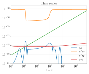
Figure 1: Ratios of the relevant scales of the problem, with respect to the dominant one: the electrical resistivity $\eta$. During the period of interest the next scale in the hierarchy is the Coulomb time scale. Early enough in time, Thomson scattering becomes more efficient than Coulomb scattering.

There is a very strong hierarchy of scales, with $\eta\ll\tau_{C}\ll\tau_{T},\mathcal{H}^{-1},\alpha^{-1}$. In the next section, we will use this fact to find an approximate solution of the system.

Production mechanism.

The main physical mechanisms at work can be nicely illustrated analyzing the behaviour of the bulk velocities. The relevance of the previous time scales will be made explicit if we write the equations in terms of $e^{i}_{(\beta)}$, where $\mathcal{E}_{(\beta)}^{i}=a^{5/2}n_{e}\tau_{C}\,e^{i}_{(\beta)}$. At the background level, the leading $\mathcal{O}\!\left(\beta\right)$ piece of (Plasma system.), plus the relevant Maxwell equation, yields

$$\Delta\dot{\beta}_{ep}^{i}+\left(\frac{1}{\tau_{c}}+\alpha+\mathcal{H}\right)\Delta\beta^{i}_{ep}+\frac{1}{a^{1/2}\eta}e^{i}_{(\beta)} =\mathcal{T}^{i}_{\beta}\ ,$$ (14a)

$$\dot{e}^{i}_{(\beta)}-\frac{a^{1/2}}{\tau_{c}}\Delta\beta_{ep}^{i} =0\ ,$$ (14b)

where the Thomson dragging term is $\mathcal{T}^{i}_{\beta}\equiv\frac{4}{3\tau_{T}}\Delta\beta^{i}_{\gamma e}$. The result is a very simple dynamical system where, as discussed in the previous section, the strong hierarchy of scales present in the problem allows us to simplify the analysis keeping only the leading $\mathcal{O}\!\left(\eta\right)$ behaviour. The homogeneous part of this system (without the source) corresponds to the usual electron-proton plasma (without photons). If the system is placed out of the equilibrium $\Delta\beta_{ep}^{i}=e_{(\beta)}^{i}=0$ configuration, an electric field is created in response, acting as a restoring force. The homogeneous solutions oscillate with characteristic frequency $\omega\simeq 1/\sqrt{\eta\,\tau_{C}}$ and are damped with a damping coefficient $\Gamma\simeq 1/2\tau_{C}$. The presence of photons modifies this picture. Due to the large mass difference, $m_{p}\gg m_{e}$, the Thomson coupling of photons to electrons is much more effective than to protons, producing a differential dragging and introducing the source $\mathcal{T}^{i}_{\beta}$. The particular solution of the system (14) can be found to be

$$\Delta\beta^{i}_{ep} =\eta\,\tau_{C}\,\dot{\mathcal{T}}^{i}_{\beta}+\mathcal{O}\!\left(\eta^{2}\right)\ ,$$ (15a)

$$e^{i}_{(\beta)} =a^{1/2}\,\eta\,\mathcal{T}^{i}_{\beta}+\mathcal{O}\!\left(\eta^{2}\right)\ .$$ (15b)

This is the essence of the Harrison mechanism: the Thomson dragging of the photons produces an electric field proportional to the photon-baryon velocity difference. Notice that a homogeneous electric field is generated, pointing in the bulk flow direction and with a small amplitude $\mathcal{E}_{(\beta)}\lesssim 10^{-30}\ \text{G}(1+z)^{2}$, according to the current Planck limits for $\beta$. The same kind of analysis can be carried out to prove that $\Delta n_{ep},\Delta v_{ep}^{i}=\mathcal{O}\!\left(\eta\,\tau_{C}\right)$ and from (Plasma system.) we get the leading order result

$$\delta\mathcal{E}^{i}=\frac{a}{en_{e}}C^{i}_{e\gamma}-\delta_{n_{e}}\mathcal{E}^{i}_{(\beta)}+\mathcal{O}\!\left(\eta\right)\ .$$ (16)

In Fourier space, we decompose the velocity and the electromagnetic fields into vortical and longitudinal components as

$$\delta\boldsymbol{v}_{s} =\chi_{s}\left(\hat{\beta}-(\hat{\beta}\cdot\hat{k})\,\hat{k}\right)-\frac{\text{i}}{k}\theta_{s}\,\hat{k}\ ,$$ (17a)

$$\boldsymbol{\mathcal{E}} =\mathcal{E}^{\bot}\left(\hat{\beta}-(\hat{\beta}\cdot\hat{k})\,\hat{k}\right)+\mathcal{E}^{\parallel}\,\hat{k}\ ,$$ (17b)

$$\boldsymbol{\mathcal{B}} =\text{i}\,\mathcal{B}\left(\hat{\beta}\wedge\hat{k}\right)\ .$$ (17c)

From the Maxwell equations, including perturbations, we have

$$\dot{\mathcal{B}}=-k\,\delta\mathcal{E}^{\bot}+k\phi\,\mathcal{E}_{(\beta)}^{\bot}\ .$$ (18)

Plugging in the expression obtained for the electric field (16) and written in terms of the physical magnetic field $\boldsymbol{B}\equiv a^{-2}\boldsymbol{\mathcal{B}}$, that can be obtained projecting with the tetrad of a locally inertial observer Durrer and Neronov (2013), Eq. (18) reads

$$\frac{\text{d}}{\text{d}\tau}\left(a^{2}B\right)=-\frac{4a^{2}k\sigma_{T}\rho_{\gamma}}{3e}\Big{(} \Delta\chi_{\gamma e}+\beta_{e}(\delta_{n_{e}}-\delta_{\gamma})$$

$$+\Delta\beta_{\gamma e}(\psi-\phi)\Big{)}\ .$$ (19)

This is the final equation governing the production of magnetic fields. It generalizes the Harrison mechanism to the case in which there are bulk flows in the plasma. It is also analogous to the one obtained in previous studies of production of magnetic fields in second order cosmological perturbation theory Fenu et al. (2011); Saga et al. (2015). Details on the evolution of the cosmological bulk flows $\beta$, and the vorticity produced by these flows can be found in Cembranos et al. (2019).

Evolution and results.

The magnetic field power spectrum is defined by

$$\left\langle B_{i}(z,\boldsymbol{k})B_{j}^{*}(z,\boldsymbol{k}^{\prime})\right\rangle=\delta(\boldsymbol{k}-\boldsymbol{k}^{\prime})(\hat{\beta}\wedge\hat{k})_{i}(\hat{\beta}\wedge\hat{k})_{j}P_{B}(z,k)\,,$$ (20)

as

$$P_{B}(z,k)=|T_{B}(z,k)|^{2}\frac{2\pi^{2}}{k^{3}}\mathcal{P}_{\mathcal{R}}(k)\ ,$$ (21)

where $\mathcal{P}_{\mathcal{R}}(k)$ is the usual nearly scale-invariant primordial curvature power spectrum and $T_{B}(z,k)$ is the magnetic field transfer function computed using (Production mechanism.). In Figs. 2 and 3 the comoving magnetic field $(1+z)^{-2}|T_{B}|\mathcal{P}_{\mathcal{R}}^{1/2}$ is plotted as a function of redshift and scale respectively.

There are two points worth emphasizing. On the one hand, the magnetic power spectrum on small and large scales has a power-law behaviour

$$\sqrt{k^{3}P_{B}(z<100,k)}\propto\left\{\begin{array}[]{l}k^{1.2}\ ,\quad k\gg 0.1\ \text{Mpc}^{-1},\\[2.56073pt] k^{2.8}\ ,\quad k\ll 0.1\ \text{Mpc}^{-1},\end{array}\right.$$ (22)

so that the magnetic field is steeply rising as $k^{1.2}$ on small scales, until the turbulence scale kicks in. On the other hand, the comoving magnetic field is continuously produced, with an important boost at recombination and remaining essentially constant for $z<100$.

Following Fenu et al. (2011), we also define the magnetic field smoothed over a comoving scale $L$ as

$$B_{L}^{2}(z)=\frac{1}{2\pi^{2}}\int^{\infty}_{0}\text{d}k\,k^{2}P_{B}(z,k)\exp\left(-\frac{k^{2}L^{2}}{2}\right)\ .$$ (23)

Figure 2: Comoving magnetic field as a function of the scale for different redshifts. Notice that the $z=0$ and $z=10$ curves overlap. Even though there is an important production immediately after decoupling, afterwards the comoving magnetic field is constant at all scales and it is not affected by reionization.

Figure 3: Comoving magnetic field as a function of the redshift for different scales. The magnetic field presents some features inherited from the acoustic oscillations before decoupling. The main production takes place during and immediately after decoupling. Once the photon-baryon plasma is decoupled, the comoving magnetic field is constant.

Figure 4: Physical magnetic field smoothed over a given scale $L$. It is evaluated at a redshift $z=10$, where the dynamo mechanism should begin to operate Widrow (2002). Since the comoving field is constant at late times, the results can be easily rescaled to any redshift.

The magnetic field $B_{L}$ at the time of galaxy formation $z_{\text{gf}}=10$ is depicted in Fig. 4. The numerical computation of the transfer function becomes harder for smaller scales, and some of the usual approximations in CMB calculations cannot be trusted for scales $k>10\ \text{Mpc}^{-1}$ Blas et al. (2011). Therefore, we only compute the spectrum up to scales $k=9\ \text{Mpc}^{-1}$. The field $B_{L}$ can be well approximated as a power law at small scales, yielding the approximate result

$$|B_{L}(z<100)| \simeq 5.7\times 10^{-24}\ \text{G}\ \left(\frac{L}{\text{Mpc}}\right)^{-1.2}$$

$$\qquad\times\left(\frac{1+z}{11}\right)^{2}\left(\frac{\beta}{8.5\times 10^{-4}}\right)\ ,$$ (24)

for $L<1\ \text{Mpc}$ where $\beta$ is the relative bulk velocity between photons and baryons. These results show that, although the field seems too weak to directly account for the intergalactic magnetic fields or magnetic fields in voids, the mechanism proposed provides a seed field large enough to potentially explain the galactic magnetic fields, after a suitable dynamo amplification.

References

- Widrow (2002) L. M. Widrow, Rev. Mod. Phys. 74, 775 (2002), eprint astro-ph/0207240.
- Neronov and Vovk (2010) A. Neronov and I. Vovk, Science 328, 73 (2010), eprint 1006.3504.
- Banerjee and Jedamzik (2004) R. Banerjee and K. Jedamzik, Phys. Rev. D70, 123003 (2004), eprint astro-ph/0410032.
- Durrer and Neronov (2013) R. Durrer and A. Neronov, Astron. Astrophys. Rev. 21, 62 (2013), eprint 1303.7121.
- Subramanian (2016) K. Subramanian, Rept. Prog. Phys. 79, 076901 (2016), eprint 1504.02311.
- Davis et al. (1999) A.-C. Davis, M. Lilley, and O. Tornkvist, Phys. Rev. D60, 021301 (1999), eprint astro-ph/9904022.
- Turner and Widrow (1988) M. S. Turner and L. M. Widrow, Phys. Rev. D37, 2743 (1988).
- Maroto (2001) A. L. Maroto, Phys. Rev. D64, 083006 (2001), eprint hep-ph/0008288.
- Vachaspati (1991) T. Vachaspati, Phys. Lett. B265, 258 (1991).
- Quashnock et al. (1989) J. M. Quashnock, A. Loeb, and D. N. Spergel, Astrophys. J. 344, L49 (1989).
- Harrison (1970) E. Harrison, Monthly Notices of the Royal Astronomical Society 147, 279 (1970).
- Rees (1987) M. J. Rees, Q. J. R. Astron. Soc. 28, 197 (1987).
- Ichiki et al. (2012) K. Ichiki, K. Takahashi, and N. Sugiyama, Phys. Rev. D85, 043009 (2012), eprint 1112.4705.
- Hollenstein et al. (2008) L. Hollenstein, C. Caprini, R. Crittenden, and R. Maartens, Phys. Rev. D77, 063517 (2008), eprint 0712.1667.
- Takahashi et al. (2005) K. Takahashi, K. Ichiki, H. Ohno, and H. Hanayama, Phys. Rev. Lett. 95, 121301 (2005), eprint astro-ph/0502283.
- Fenu et al. (2011) E. Fenu, C. Pitrou, and R. Maartens, Mon. Not. Roy. Astron. Soc. 414, 2354 (2011), eprint 1012.2958.
- Saga et al. (2015) S. Saga, K. Ichiki, K. Takahashi, and N. Sugiyama, Phys. Rev. D91, 123510 (2015), eprint 1504.03790.
- Cembranos et al. (2019) J. A. R. Cembranos, A. L. Maroto, and H. Villarrubia-Rojo, JCAP 1906, 041 (2019), eprint 1903.11009.
- Kashlinsky et al. (2009) A. Kashlinsky, F. Atrio-Barandela, D. Kocevski, and H. Ebeling, Astrophys. J. 686, L49 (2009), eprint 0809.3734.
- Atrio-Barandela et al. (2015) F. Atrio-Barandela, A. Kashlinsky, H. Ebeling, D. J. Fixsen, and D. Kocevski, Astrophys. J. 810, 143 (2015), eprint 1411.4180.
- Ade et al. (2014) P. A. R. Ade et al. (Planck), Astron. Astrophys. 561, A97 (2014), eprint 1303.5090.
- Scrimgeour et al. (2016) M. I. Scrimgeour et al., Mon. Not. Roy. Astron. Soc. 455, 386 (2016), eprint 1511.06930.
- Blas et al. (2011) D. Blas, J. Lesgourgues, and T. Tram, JCAP 1107, 034 (2011), eprint 1104.2933.