Robust and Fast Automatic Modulation Classification with CNN under Multipath Fading Channels

Abstract

Automatic modulation classification (AMC) has been studied for more than a quarter of a century; however, it has been difficult to design a classifier that operates successfully under changing multipath fading conditions and other impairments. Recently, deep learning (DL)–based methods are adopted by AMC systems and major improvements are reported. In this paper, a novel convolutional neural network (CNN) classifier model is proposed to classify modulation classes in terms of their families, i.e., types. The proposed classifier is robust against realistic wireless channel impairments and in relation to that, when the data sets that are utilized for testing and evaluating the proposed methods are considered, it is seen that RadioML2016.10a is the main dataset utilized for testing and evaluation of the proposed methods. However, the channel effects incorporated in this dataset and some others may lack the appropriate modeling of the real–world conditions since it only considers two distributions for channel models for a single tap configuration. Therefore, in this paper, a more comprehensive dataset, named as HisarMod2019.1, is also introduced, considering real-life applicability. HisarMod2019.1 includes $26$ modulation classes passing through the channels with $5$ different fading types and several number of taps for classification. It is shown that the proposed model performs better than the existing models in terms of both accuracy and training time under more realistic conditions. Even more, surpassed their performance when the RadioML2016.10a dataset is utilized.

I Introduction

AMC has been considered as an important part of various military and civilian communication systems, such as electronic warfare, radio surveillance and spectrum awareness. As known, classical signal identification methods used in the past are based on complex collections of feature extraction methods, such as cyclostationarity, high–order cumulants and complex hierarchical decision trees. Furthermore, it should be noted that classical methods cannot be generalized over all signal types and they suffer from dynamic nature of the propagation channel and cannot be adopted easily if a new wireless communication technology emerges. On the other hand, DL has been proposed as a useful method for such classification problems and recently have been applied to this domain intensively. However, these methods should also provide strong performance against the wireless impairments in that particular domain thus, robust AMC methods based on DL techniques should be investigated to achieve dependable, efficient and resilient classification performance under realistic wireless communication channel conditions.

I-A Related Work

Signal identification systems often use likelihood based (LB) and feature based (FB) techniques. Although, LB methods make the probability of correct classification maximum, they suffer from high computational complexity. Also, they are not robust to model mismatches, such as channel coefficient estimates and timing offsets [1, 2, 3].

On the other hand, in FB approaches, it is required to find a feature which can distinguish the signal from others. However, single feature mostly is not sufficient to classify signals in a large set. In literature, the higher order statistics, wavelet transform, and cyclic characteristics are mainly proposed features for signal identification. For instance, the wavelet transform is utilized in the identification of frequency shift keying (FSK) and phase shift keying (PSK) signals [4]. The higher order statistics such as higher order cumulants and moments which are another feature used in AMC [5, 6]. In addition to these features, [7] utilizes instantaneous amplitude, phase and frequency statistics in order to make modulation classification. Howbeit, it is explicitly known that these features hamper to perform well in real–world conditions such as multipath channel fading, frequency, and timing offsets. Although the most powerful FB approach, cyclostationarity–based features are resistant to mismatches compared to other features [8], it suffers from high computational complexity.

Machine learning–based approaches have been recently adopted to AMC. For example, CNN, convolutional long short term memory fully connected deep neural network (CLDNN) and long short term memory (LSTM) can be said as the most popular deep neural network architectures for AMC. [9] proposes using CNN with in–phase/quadrature (I/Q) data and fast Fourier Transform (FFT) for AMC and interference identification in industrial, scientific and medical (ISM) band. It is shown that recurrent neural networks can be utilized for AMC under Rayleigh channel with uncertain noise condition [10]. In addition to proposing CLDNN for AMC, [11] compares it to other existing models under different subsampling rates and different number of samples. Furthermore, it aims to reduce training time for online learning by utilizing subsampling and principal component analysis (PCA). LSTM is proposed in [12], but it does not allow online learning and has long enough training time to require very high computing capacity. The RadioML2016.10a dataset [13] is widely used in the literature. However, a system that works under real–conditions should be designed to operate under different channel conditions. Due to the dynamic nature of propagation channel and severe multipath effects, the existing available datasets cannot fulfill to provide the desired real–world conditions. RadioML2018.01a introduced in [14] includes over–the–air recordings of $24$ digital and analog modulation types. However, it cannot provide information about the channel parameters since this data set is based on measurement. Therefore, this dataset cannot allow generating information about how the channel conditions affect the performance of the model trained on the dataset. Furthermore, it has not serious diversity because it is created in the laboratory environment where there is no significant change in the channel parameters such as fading and number of taps. In this case, there is a need for a data set that includes both actual channel conditions and controlled channel parameters. It is also necessary to design a DL model that can work under real channel conditions.

I-B Contributions

The main contributions of this study are two fold and can be summarized as follows:

• First, aforementioned discussions show that currently, there is no comprehensive, inclusive, and controlled dataset that integrates the severe multipath effects for the real–world channel conditions. Therefore, we first introduce a new and more challenging modulation dataset, HisarMod2019.1 [15]. This new public dataset provides wireless signals under ideal, static, Rayleigh, Rician ($k=3$), and Nakagami–m ($m=2$) channel conditions with various numbers of channel taps. Thus, it becomes possible to observe more realistic channel conditions for the proposed DL–based AMC methods.

• More importantly, a new CNN model with optimal performance in terms of accuracy and training time under more realistic conditions is proposed. The proposed method exhibits higher performance under both in HisarMod2019.1 dataset and existing RadioML2016.10a dataset when compared to the available classifiers. The new CNN consists of four convolution and two dense layers. In addition to its high performance, the model has lower training complexity when compared to the available techniques, thus, the training process is relatively short.

II HisarMod2019.1: A New Dataset

In order to increase the diversity in signal datasets, we create a new dataset called as HisarMod2019.1, which includes $26$ classes and $5$ different modulation families passing through $5$ different wireless communication channel. During the generation of the dataset, MATLAB 2017a is employed for creating random bit sequences, symbols, and wireless fading channels.

The dataset includes $26$ modulation types from $5$ different modulation families which are analog, FSK, pulse amplitude modulation (PAM), PSK, and quadrature amplitude modulation (QAM). All modulation types are listed in Table I. In the dataset, there are $1500$ signals, which have the length of $1024$ I/Q samples, for each modulation type. To make HisarMod2019.1 similar to RadioML2016.10a for fair comparison, there are $20$ different signal–to–noise ratio (SNR) levels in between -20dB and 18dB. As a result, the dataset covers totally $780000$ signals. When generating signals, oversampling rate is chosen as $2$ and raised cosine pulse shaping filter is employed with roll–off factor of $0.35$.

Furthermore, the dataset consists of signals passing through $5$ different wireless communication channels which are ideal, static, Rayleigh, Rician ($k=3$), and Nakagami–m ($m=2$). These channels are equally likely distributed over the dataset; therefore, there are 300 signals for each modulation type and each SNR level. Ideal channel refers that there is no fading, but additive white Gaussian noise (AWGN). In the static channel, the channel coefficients are randomly determined at the beginning and they remain constant over the propagation time. The signals passing through Rayleigh channel are employed to make the system resistant against non line–of–sight (NLOS) conditions. On the other hand, Rician fading with shape parameter, $k$, of $3$ is utilized owing to the fact that the dataset covers a mild fading. In addition to these channel models, the distribution of received power is selected as Nakagami–m with shape parameter, $m$, of $2$ for the rest of the signals in the dataset. As a result, the dataset includes signals with different fading models. Noting that the number of multipath channel taps are equally likely selected as $4$ and $6$ which are adopted from ITU–R M1225 [16].

TABLE I: HisarMod2019.1 includes 26 different modulation types from 5 different modulation families.

Modulation Family	Modulation Types
Analog	AM–DSB
	AM–SC
	AM–USB
	AM–LSB
	FM
	PM
FSK	2–FSK
	4–FSK
	8–FSK
	16–FSK
PAM	4–PAM
	8–PAM
	16–PAM
PSK	BPSK
	QPSK
	8–PSK
	16–PSK
	32–PSK
	64–PSK
QAM	4–QAM
	8–QAM
	16–QAM
	32–QAM
	64–QAM
	128–QAM
	256–QAM

III The Proposed CNN Model

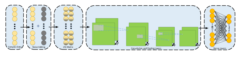
Figure 1: The proposed CNN model consists of four convolution and pooling layers and two dense layers.

In this paper, a CNN model is built by using Keras which is an open source machine learning library [17]. The proposed CNN model involves four convolution and pooling layers terminated by two dense layers. The rectified linear unit (ReLU) activation function, which is defined as

$$x_{out}=\max(0,\,\omega x_{in}+b),$$ (1)

is employed in each convolution layer. In (1), $x_{in}$, $x_{out}$, $\omega$, and $b$ are the input and output of the function, weight, and bias, respectively. In this model, it is chosen that the model gets narrower in terms of the number of filters in each convolution layer through the end of the feature extraction part of the model. Our experience with many different configurations indicated that the models that get narrower in each following convolutional layer provides better results in terms of classification and reduce training time. Indeed, for the optimal performance, we employed $256$ filters in the first layer while the last layer had $64$ filters. The first dense layer is formed by $128$ neurons and ReLU activation function. The dense layer is followed by a softmax activation function which computes the probabilities for each class as

$$S\left(y_{i}\right)=\frac{e^{y_{i}}}{\sum_{j}e^{y_{j}}},\;i,\,j=1,2,\cdots,N,$$ (2)

where $y_{i}$ and $N$ are any element of classes and the number of classes, respectively. Moreover, the adaptive moment estimation (ADAM) optimizer is used to estimate the model parameters with the learning rate of $10^{-4}$. The CNN model architecture is depicted in Fig. 1. Furthermore, the layout for the proposed CNN model is given in Table II. During the training process, we use early stopping to terminate the process if the validation loss converges to a level enough. As a result, the model is preserved to be overfitted. As seen in Fig. 1, there is a layer, which adds noise at each epoch; thus, it also prevents the model to overfit. The power of noise is determined according to the desired SNR level.

In the training and test stages, we employ four NVIDIA Tesla V100 graphics processing units by operating them in parallel. It is seen that the proposed CNN model is too light compared to CLDNN [11] and LSTM [12]. For example, the proposed CNN model has $15$ million trainable parameters, whereas CLDNN has $27$ million trainable parameters for HisarMod2019.1 dataset. Furthermore, CNN model takes one–quarter time of LSTM per epoch.

TABLE II: The proposed CNN layout for the proposed dataset HisarMod2019.1 and RadioML2016.10a.

Layer	Output Dimensions
	HisarMod2019.1	RadioML2016.10a
Input	$2\times 1024$	$2\times 128$
Noise Layer	$2\times 1024$	–
Conv1	$2\times 1024\times 256$	$2\times 128\times 256$
Max_Pool1	$2\times 512\times 256$	$2\times 64\times 256$
Dropout1	$2\times 512\times 256$	$2\times 64\times 256$
Conv2	$2\times 512\times 128$	$2\times 64\times 128$
Max_Pool2	$2\times 256\times 128$	$2\times 32\times 128$
Dropout2	$2\times 256\times 128$	$2\times 32\times 128$
Conv3	$2\times 256\times 64$	$2\times 32\times 64$
Max_Pool3	$2\times 128\times 64$	$2\times 16\times 64$
Dropout3	$2\times 128\times 64$	$2\times 16\times 64$
Conv4	$2\times 128\times 64$	$2\times 16\times 64$
Max_Pool4	$2\times 64\times 64$	$2\times 8\times 64$
Dropout4	$2\times 64\times 64$	$2\times 8\times 64$
Flatten	$8192$	$1024$
Dense1	$128$	$128$
Dense2	$5$	$10$
Trainable Par.	$15,764,53$	$6,595,94$

IV Classification Results

The proposed model is tested in both the HisarMod2019.1 and the RadioML2016.10a datasets. The test results are provided below.

IV-A HisarMod2019.1 Dataset Classification Results

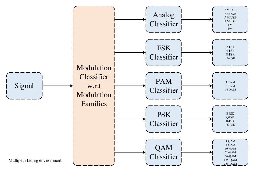
Figure 2: In the multipath fading environment, it is not easy to deal with a large dataset; hence, it can be handled in two steps: modulation family classification, and modulation type classification.

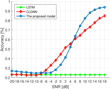
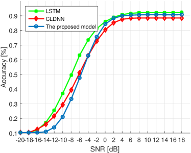
Figure 3: The accuracy values for LSTM, CLDNN and the proposed CNN models in (a) the HisarMod2019.1, (b) RadioML2016.10a datasets.

As detailed in Section II, the HisarMod2019.1 covers $26$ different modulation types. It is not that easy to handle so many signal types in the fading environment. It is expected that they are confused each other due to the deterioration in their amplitude and phase. Thus, in this study, we use an approach like the data binning method by labeling signals with respect to their modulation families such as analog, FSK, PAM, PSK, and QAM. The hierarchical approach is depicted in Fig. 2. Firstly, we aim to classify signals in terms of modulation families. Then, each modulation type can be identified in the family subset. One should keep in mind that this study focuses on the classification of the modulation families not the order of each modulation type for the HisarMod2019.1 dataset. The dataset is split as $8/15$, $2/15$, and $5/15$ for training, validation, and test sets, respectively.

As stated before, the early stopping is employed in the training stage. The first layer of the CNN adds noise to data according to the SNR level. As a result, the model becomes more robust to overfitting.

The model gives meaningful results at SNR levels higher than $2$ dB. It might be said that the model makes a random choice between modulation families at low SNR values. Considering the nature of wireless communications, the model performs well for the expected SNR values. The dataset is also employed with the CLDNN model. It is noted that we employ the CLDNN and LSTM models as detailed in [11] and [12] without any adjustment. Also, the proposed CNN model shows better performance than the existing CLDNN and LSTM models in HisarMod2019.1 dataset. For example, it exceeds $80\%$ accuracy at 8dB SNR; however, CLDNN performs with the same accuracy at 16dB SNR. While CLDNN does not achieve $90\%$ accuracy, our model exceeds this level at 14dB and higher. The maximum accuracy values for the proposed CNN model and state of the art CLDNN model are $94\%$ and $85\%$, respectively. Surprisingly, LSTM cannot show acceptable classification results; however, it performs well in RadioML2016.10a. At SNR values, the results are not meaningful in terms the classification accuracy since the false alarm rate gets higher. Fig. 3 denotes the accuracy values for CNN, CLDNN, and LSTM models at the SNR values in between [-20dB, 18dB]. Fig. 4 and Fig. 5 show the confusion matrices for the proposed CNN model and CLDNN model, respectively. Both of them have difficulty in the identification of QAM signals. On the other hand, LSTM recognizes signals as analog modulated signals regardless of the received signal type. Hence, the confusion matrices are not provided for the LSTM model.

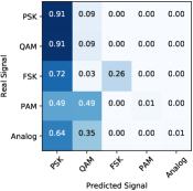
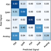
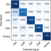
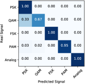
Figure 4: The confusion matrices of the proposed CNN model test results at (a) 0dB, (b) 6dB, (c) 12dB, (d) 18dB, when the HisarMod2019.1 dataset is used.

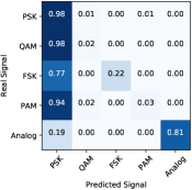
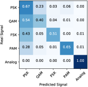
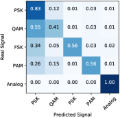
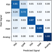
Figure 5: The confusion matrices of the CLDNN model test results at (a) 0dB, (b) 6dB, (c) 12dB, (d) 18dB, when the HisarMod2019.1 dataset is used.

IV-B RadioML2016.10a Dataset Classification Results

RadioML dataset is heavily used in modulation classification studies and it is a well accepted dataset by the literature. Therefore, in order to show the robustness of our proposed CNN model, we also test our model in RadioML dataset to observe its performance. In this section, RadioML2016.10a dataset is employed. It consists of synthetic signals with $10$ modulation types. The modulation types covered by the dataset are listed as: AM–DSB, WBFM, GFSK, CPFSK, 4–PAM, BPSK, QPSK, 8–PSK, 16–QAM, and 64–QAM. Details for the generation and packaging of the dataset can be found in [13].

Here, the dataset is split into two parts (i.e. training and test) with equal number of signals. After training procedure, the models are tested with the rest of the signals. According to test results, the proposed CNN model shows higher performance than the CLDNN model at the SNR levels higher than -2dB. LSTM performs slightly better than CNN. The CLDNN is able to reach the maximum accuracy of $88.5\%$. On the other hand, the proposed CNN model performs with the maximum accuracy of $90.7\%$ even though it is not originally designed for the RadioML2016.10a dataset. Although LSTM reaches up to $92.3\%$ accuracy, its computational complexity is extremely high. Fig. 3 denotes the accuracy values with respect to SNR levels. The confusion matrices for the classification results of the proposed CNN model are depicted in Fig. 6. It is observed that the model recognizes almost all signals as 8–PSK at low SNR levels. Fig. 6 shows the confusion matrix of the minimum SNR value of which the model performs over $50\%$ accuracy. As can be seen from Fig. 6, the model gives poor results in modulation types other than 4–PAM. The proposed model achieves very high performance in all modulation types, except WBFM at 6dB and above.

Initial observations suggest that the proposed model can work with high performance both in a diverse dataset, HisarMod2019.1, and RadioML2016.10a which is a frequently used dataset.

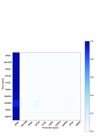
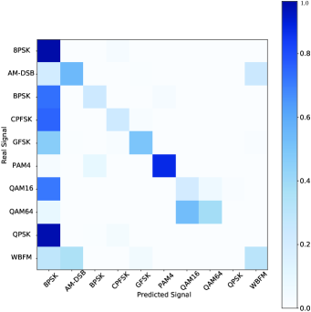
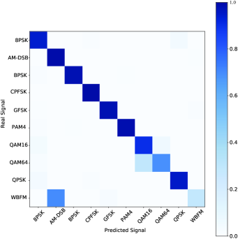
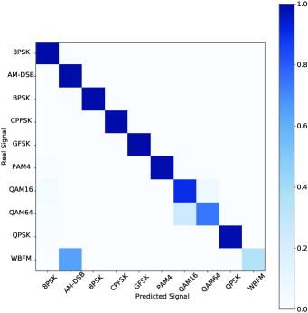
Figure 6: The confusion matrices of the proposed CNN model test results at (a) -12dB, (b) -6dB, (c) 0dB, (d) 6dB, when the RadioML2016.10a dataset is used.

V Concluding Remarks

In this study, we present a diverse new dataset, which consists of multipath fading signals with different number of channel taps, and a CNN model for AMC. The first stage of hierarchical classification architecture, which is the classification of modulation families, is realized with the proposed CNN model on this dataset and the results compared with the CLDNN model proposed in the literature. The results show that the proposed CNN model performs significantly better than CLDNN. Furthermore, the performance of the proposed CNN model on the RadioML2016.10a dataset is examined. It is demonstrated that the proposed CNN model is both faster and more accurate than the CLDNN model. As a future work, we will investigate the classification of modulation orders assuming that the modulation family is identified. Finally, extensive search conducted for optimal model in this study shows that starting with an extensive set of filters, and then reducing their numbers down step by step provides better results in terms of accuracy. This phenomenon will be investigated thoroughly and technical discussions will be provided in terms of explainable AI terminology.

References

- [1] P. Panagiotou, A. Anastasopoulos, and A. Polydoros, “Likelihood ratio tests for modulation classification,” in IEEE Mil. Commun. Conf. (MILCOM), vol. 2, 2000, pp. 670–674.
- [2] F. Hameed, O. A. Dobre, and D. C. Popescu, “On the likelihood-based approach to modulation classification,” IEEE Trans. Wireless Commun., vol. 8, no. 12, pp. 5884–5892, 2009.
- [3] J. L. Xu, W. Su, and M. Zhou, “Software-defined radio equipped with rapid modulation recognition,” IEEE Trans. Veh. Technol., vol. 59, no. 4, pp. 1659–1667, 2010.
- [4] L. Hong and K. Ho, “Identification of digital modulation types using the wavelet transform,” in IEEE Mil. Commun. Conf. (MILCOM), vol. 1, 1999, pp. 427–431.
- [5] L. Liu and J. Xu, “A novel modulation classification method based on high order cumulants,” in Intl. Conf. on Wireless Commun., Net. and Mobile Computing (WiCOM), 2006, pp. 1–5.
- [6] A. Swami and B. M. Sadler, “Hierarchical digital modulation classification using cumulants,” IEEE Trans. Commun., vol. 48, no. 3, pp. 416–429, 2000.
- [7] A. Nandi and E. E. Azzouz, “Automatic analogue modulation recognition,” Signal Processing, vol. 46, no. 2, pp. 211–222, 1995.
- [8] O. A. Dobre, “Signal identification for emerging intelligent radios: Classical problems and new challenges,” IEEE Instrum. Meas. Mag., vol. 18, no. 2, pp. 11–18, 2015.
- [9] M. Kulin, T. Kazaz, I. Moerman, and E. De Poorter, “End-to-end learning from spectrum data: A deep learning approach for wireless signal identification in spectrum monitoring applications,” IEEE Access, vol. 6, pp. 18 484–18 501, 2018.
- [10] S. Hu, Y. Pei, P. P. Liang, and Y.-C. Liang, “Robust modulation classification under uncertain noise condition using recurrent neural network,” in IEEE Glob. Commun. Conf. (GLOBECOM), 2018, pp. 1–7.
- [11] S. Ramjee, S. Ju, D. Yang, X. Liu, A. E. Gamal, and Y. C. Eldar, “Fast deep learning for automatic modulation classification,” arXiv preprint arXiv:1901.05850, 2019.
- [12] S. Rajendran, W. Meert, D. Giustiniano, V. Lenders, and S. Pollin, “Deep learning models for wireless signal classification with distributed low-cost spectrum sensors,” IEEE Trans. on Cogn. Commun. Netw., vol. 4, no. 3, pp. 433–445, 2018.
- [13] T. J. O’shea and N. West, “Radio machine learning dataset generation with GNU radio,” in Proceedings of the GNU Radio Conference, vol. 1, no. 1, 2016.
- [14] T. J. O’Shea, T. Roy, and T. C. Clancy, “Over-the-air deep learning based radio signal classification,” IEEE J. Sel. Topics Signal Process., vol. 12, no. 1, pp. 168–179, 2018.
- [15] “Hisarmod: A new challenging modulated signals dataset,” 2019. [Online]. Available: http://dx.doi.org/10.21227/8k12-2g70
- [16] R. I.-R. M. ITU, “Guidelines for evaluation of radio transmission technologies for IMT-2000,” 1997. [Online]. Available: https://www.itu.int/dms_pubrec/itu-r/rec/m/R-REC-M.1225-0-199702-I!!PDF-E.pdf
- [17] F. Chollet et al., “Keras,” https://keras.io, 2015.