Time-resolved photometry of the young dipper RX J1604.3-2130A:

Abstract

Context. RX J1604.3-2130A is a young, dipper-type, variable star in the Upper Scorpius association, suspected to have an inclined inner disk with respect to its face-on outer disk.

Aims. We study the eclipses to constrain the inner disk properties.

Methods. We use time-resolved photometry from the Rapid Eye Mount telescope and Kepler 2 data to study the multi-wavelength variability, and archival optical and IR data to track accretion, rotation, and changes in disk structure.

Results. The observations reveal details of the structure and matter transport through the inner disk. The eclipses show 5d quasi-periodicity, with the phase drifting in time and some periods showing increased/decreased eclipse depth and frequency. Dips are consistent with extinction by slightly processed dust grains in an inclined, irregularly-shaped inner disk locked to the star through two relatively stable accretion structures. The grains are located near the dust sublimation radius ($\sim$0.06 au) at the corotation radius, and can explain the shadows observed in the outer disk. The total mass (gas and dust) required to produce the eclipses and shadows is a few % of a Ceres mass. Such amount of mass is accreted/replenished by accretion in days to weeks, which explains the variability from period to period. Spitzer and WISE variability reveal variations in the dust content in the innermost disk on a few years timescale, which is consistent with small imbalances (compared to the stellar accretion rate) in the matter transport from the outer to the inner disk. A decrease in the accretion rate is observed at the times of less eclipsing variability and low mid-IR fluxes, confirming this picture. The v$sini$=16 km/s confirms that the star cannot be aligned with the outer disk, but is likely close to equator-on and to be aligned with the inner disk. This anomalous orientation is a challenge for standard theories of protoplanetary disk formation.

1 Introduction

Dippers, also called AA Tau-type stars, are young stars with lightcurves characterized by aperiodic dimmings or eclipsing events consistent with variable extinction by circumstellar material (Bouvier et al., 1999). Dippers are particularly interesting sources because the occultations of the star by the disk material offer an opportunity to explore the structure and composition of the innermost disk (Schneider et al., 2018) that are inaccessible for most other sources.

RX J1604.3-2130A is a solar-type star in the 5-11 Myr old Upper Scorpius Association (Preibisch & Zinnecker, 1999; Pecaut et al., 2012; Pecaut, & Mamajek, 2016) that has been identified as a dipper (Ansdell et al., 2016). It possesses one of the brightest disks detected in the region, which also has a large inner cavity (Carpenter et al., 2006, 2009; Dahm, & Carpenter, 2009; Mathews et al., 2012; Carpenter et al., 2014; Zhang et al., 2014; Dong et al., 2017), being considered as a transition disk. The resolved outer disk is nearly face-on, with an estimated inclination of 6 deg (Zhang et al., 2014; Dong et al., 2017). The disk contains a substantial amount of gas (Mathews et al., 2013), although the cavity shows significant CO depletion (Dong et al., 2017; Mayama et al., 2018).

The disk gap could be the result of planetary formation or of the presence of a yet-undetected stellar companion. A low-mass (M2) companion, which is itself a binary with a stellar companion at 0.082 arcsec (Köhler et al., 2000), is found at 16” (RX J1604.3-2130B). Considering the Gaia DR2 parallax (6.662$\pm$0.057 arcsec; Gaia Collaboration et al., 2016, 2018) available through VizieR (Gaia Collaboration, 2018), its distance is 150$\pm$1 pc, which implies that the potential companions are located at about 2400 au and 12 au (from B), respectively. Nearby companions of RX J1604.3-2130A at $>$22 au have been excluded down to 2-3 M_J (Kraus et al., 2008; Canovas et al., 2017), but there is no record of objects in the innermost region of the gap.

The disk was observed with VLT/SPHERE, revealing a close-to-face-on ring in scattered light about 65 au in radius (Pinilla et al., 2015, 2018). Dark dents on the scattered light image of the disk rim suggested shadows cast by a highly misaligned inner disk (as it has been observed in other systems; Marino et al., 2015; Benisty et al., 2017, 2018). The origin of the shadows in an inclined inner disk has been recently confirmed by multi-epoch scattered light observations between 2016-2017 that show that the position angle of the dips varies only slightly (with PA$\sim$83.7$\pm$13.7^o and PA$\sim$265.9$\pm$13.0^o, respectively Pinilla et al., 2018), although the morphology of the shadows is quite variable on timescales of days. The presence of a misaligned disk has been also suggested from ALMA gas observations (Mayama et al., 2018) and are also in good agreement with the eclipsing activity observed, but a classical, smooth inner disk cannot explain the optical and scattered light variability observed.

In this paper, we use ground-based optical and near-IR photometry from REM/La Silla, together with K2 data and archival photometry and spectroscopy of RX J1604.3-2130A, to explore the causes behind the observed eclipses, and to constrain the structure of the innermost disk and its variability timescales. Observations are presented in Section 2. The periodicity of the lightcurves and variability causes in terms of eclipses, accretion, rotation, and variations in the inner disk structure are analyzed in Section 3. The discussion and conclusions are presented in Sections 4 and 5.

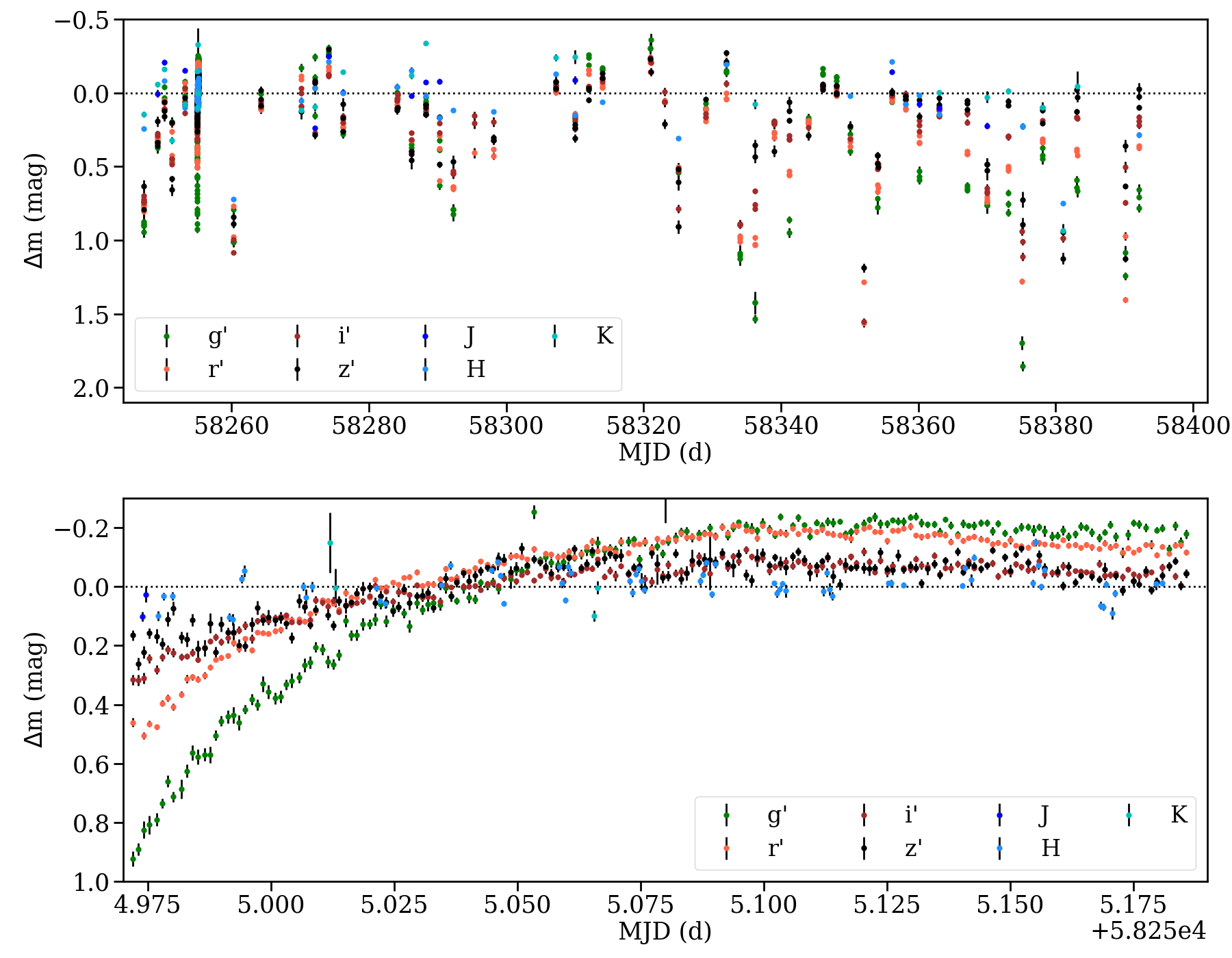
Figure 1: REM lightcurve for RX J1604.3-2130A. The upper panel shows the full lightcurve observed, while the lower panel is a zoom in the high-cadence data. All the magnitudes shown are relative magnitudes evaluated with respect to the $\sigma$-clipped average magnitude of all datapoints in each band, marked as zero point with a dotted line.

2 Observations and data reduction

2.1 REM g’r’i’z’ JHK observations

Table 1: Example of REM optical data. All magnitudes are given relative to those of 58346.021046.

MJD	$\Delta$g’	$\Delta$r’	$\Delta$i’	$\Delta$z’
(d)	(mag)	(mag)	(mag)	(mag)
58247.213152	1.031$\pm$0.051	0.782$\pm$0.015	0.774$\pm$0.025	0.658$\pm$0.044
58247.217176	1.076$\pm$0.038	0.794$\pm$0.066	0.790$\pm$0.025	0.813$\pm$0.065
58249.213074	0.505$\pm$0.037	0.340$\pm$0.019	0.343$\pm$0.021	0.218$\pm$0.034
58249.214534	0.457$\pm$0.023	0.328$\pm$0.016	0.398$\pm$0.018	0.361$\pm$0.035
58249.215942	0.464$\pm$0.028	0.330$\pm$0.015	0.327$\pm$0.016	0.382$\pm$0.036
58250.226890	0.184$\pm$0.019	0.080$\pm$0.010	0.168$\pm$0.011	0.145$\pm$0.016
58250.228301	0.164$\pm$0.017	0.089$\pm$0.008	0.159$\pm$0.013	0.084$\pm$0.030
58250.229714	0.091$\pm$0.017	0.077$\pm$0.013	0.165$\pm$0.013	0.182$\pm$0.034
58251.278677	0.599$\pm$0.020	0.447$\pm$0.013	0.499$\pm$0.011	0.606$\pm$0.021
58251.280120	0.579$\pm$0.024	0.500$\pm$0.024	0.536$\pm$0.012	0.681$\pm$0.039

RX J1604.3-2130A was observed with the Rapid Eye Mount (REM) 60cm telescope in La Silla, as part of a DDT proposal. With its two instruments, ROS2 and REMIR, REM can obtain nearly-simultaneous images in the Sloan g’,r’,i’,z’ and the IR JHK filters over a 10x10 arcmin² field. The observations took place at irregular intervals during approximately 5 months, from 2018 May 09 to 2018 October 01 (MJD 58247.21 - 58392.08). The observations were repeated at intervals between half an hour and few days, with a period of high-cadence on 58255.09 (2018 May 16-17) during which the images were taken about every 2 min. For the optical bands, a total of 338 images were obtained, among which 168 of them belong to the high-cadence dataset. The total exposure time for the optical images was 5s. Data reduction was performed with the automated REM pipeline, and the images were aligned using Astrometry.net. The IR observations were obtained during the same epochs, but due to technical issues, only 42 datasets were completed for J, 43 for K, and 142 for H. Typically, a total of 5 dithered 3s exposures were taken in each case, although some of them have less dithers if the imaging failed (especially in bad nights). Sky images were also acquired, although some of the final images have less dithers due to lack of quality of some of them. The images were reduced, combined, sky-subtracted and aligned using the automated REM pipeline, and aligned using Astrometry.net.

Aperture photometry was performed using $iraf$ task $noao.digiphot.apphot$. For the optical data, a relative calibration was performed for each filter by comparing all observations to the data taken on MJD 58346.021 (one of the best nights, based on seeing/FWHM). An iterative process based on the median and standard deviation of the magnitude difference (Sicilia-Aguilar et al., 2008, 2017) was used on all stars in the field to identify the non-variable comparison stars. The main issue is that there are few comparison stars in the field, and all of them are fainter than the target star. This is due to RX J1604.3-2130A brightness (Gaia G 11.87 mag) requiring low exposure times to avoid saturation. We thus imposed quality limits on the calibration, rejecting all those for which 4 or less comparison stars were identified and those where the calibration had magnitude-dependent offsets or very large errors. Typically, we found between 5 and 15 comparison stars for g’ and r’, and between 10 and 27 comparison stars for i’ and z’, spanning a range of 2-4 magnitudes around (but mostly fainter than) the object. The nights for which the calibration fails are typically those with poor seeing and poor weather conditions that make it hard to detect enough field stars. This results in 205 dates for which all four optical filters are complete. The final data (relative magnitudes) are listed in Table 1 with the complete table given in Appendix A. The uncertainties provided in the tables and figures include the photometric uncertainty and the uncertainty in the relative calibration. In general, the uncertainty in the relative calibration dominates the value in cases with few comparison stars.

The absolute calibration of the g’r’i’z’ data was done using griz data from PAN-STARRS (Chambers et al., 2016; Flewelling et al., 2016; Magnier et al., 2016). The procedure for the absolute calibration was similar to the relative calibration, comparing the data from MJD 58346.021 with those of PAN-STARRS. The g’r’ calibration is quite robust (2% and 4% uncertainties, respectively), but for i’ there is a large amount of scatter and for z’ only 4 reference stars could be identified. In addition, we find that there are color terms for all filters except g’. The color terms are particularly large for i’ and z’. Since there are no stars as bright as RX J1604.3-2130A in the field and very few non-variable stars in any magnitude range, the absolute calibration is very uncertain and the errors could be $>$50% in i’ and z’. The magnitudes in the reference night MJD 58346.021 are thus g’=12.47$\pm$0.02 mag, r’=11.01$\pm$0.04: mag, i’=11.7: mag, and z’=11.0: mag. Because the magnitudes in r’,i’, and z’ are estimated from much fainter stars, we label them as uncertain (:) and treat them as merely indicative, and we focus the discussion on relative REM magnitudes and relative color variations. In total, there are 261 datapoints in g’, r’ and i, and 270 in r’ observations.

For the JHK data, we followed a similar procedure. The data were calibrated against those of MJD 58363.04 (one of the best nights for which all three IR filters were obtained), which was also calibrated against 2MASS data (Skrutskie et al., 2006). The REM and 2MASS JH filters are essentially identical, while the relation between the standard Johnson K filter and the 2MASS K_s is K=K_s+0.044 mag (Bessell, 2005). The systematic errors in the absolute calibration are 4% for J and H and 2% for K. There are no evident color terms between the 2MASS and REM filters, but because the data quality of the JHK images is in general worse than in the optical, there are fewer stars for comparison. Following the same quality criteria, we only have complete JHK data on 10 epochs, although the H lightcurve is much more complete (73 points) while J and K have only 8. The final results are listed in Table 2 (complete table in Appendix A).

Table 2: Example of JHK REM observations.

MJD	J	H	K
(d)	(mag)	(mag)	(mag)
58250.227	8.920$\pm$0.020	8.205$\pm$0.007	7.895$\pm$0.012
58253.213	8.974$\pm$0.016	8.388$\pm$0.015	8.133$\pm$0.029
58272.150	9.365$\pm$0.014	8.256$\pm$0.041	8.152$\pm$0.026
58276.156	9.122$\pm$0.022	8.287$\pm$0.007	7.916$\pm$0.011
58286.128	9.145$\pm$0.018	8.135$\pm$0.023	7.938$\pm$0.024
58288.245	9.055$\pm$0.013	8.307$\pm$0.025	7.720$\pm$0.009
58309.989	9.042$\pm$0.028	8.438$\pm$0.009	7.812$\pm$0.047
58363.042	9.229$\pm$0.012	8.431$\pm$0.007	8.054$\pm$0.009

The final REM ligthcurve is displayed in Figure 1. The optical data show the typical dimming events described in Ansdell et al. (2016). The JHK data follows the behavior observed in the optical, although they are more scarce. The high-cadence data reveals the star emerging from one of the eclipses. We find that the eclipses observed by REM are deeper than previously reported (0.57 mag based on K2 data; Ansdell et al., 2016). Even though our filters are significantly narrower than the K2 filter, the maximum depth varies between 0.4–1.8 mag in g’, 0.3–1.5 mag in r’, 0.3–1.5 mag in i’, and 0.2–1.2 mag in z’. The variations in H (the only IR filter for which we have enough eclipse data) are up to 0.2-0.7 mag. There are also smaller variability events, but we detect at least 10 deep eclipses during our observations (all of which are recovered in multiple bands), in addition to other shallower ones similar to those reported by Ansdell et al. (2016). The decrease in depth with increasing wavelength suggests extinction events, which we will explore in Section 3.

2.2 Other optical lightcurves: K2 and CSS

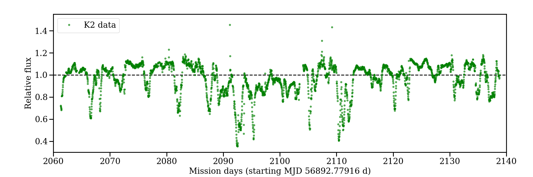
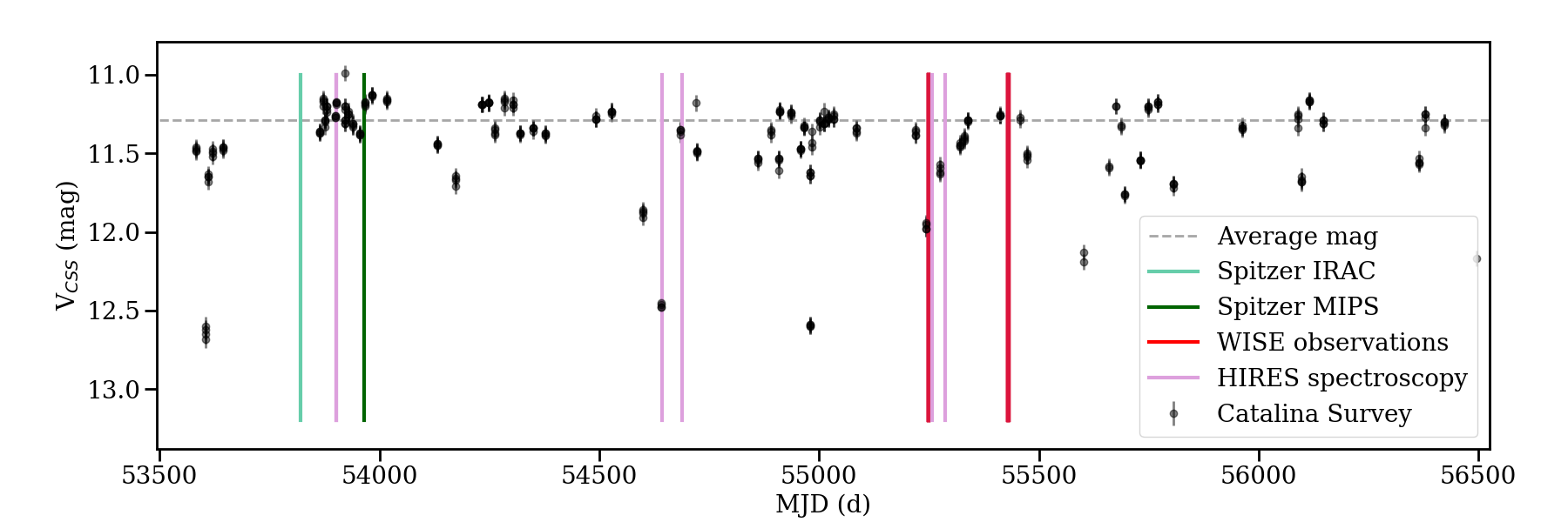
Figure 2: Top: K2 lightcurve for RX J1604.3-2130. The typical uncertainties are smaller than the dots. Bottom: Catalina Survey DR2 lightcurve. Since the Catalina data covers the epochs of the Spitzer, WISE and HIRES spectroscopy observations, we have marked them in the figure as vertical lines (see text). In both cases, the average flux (magnitude) is shown as a dotted line.

RX J1604.3-2130A was observed by K2 as part of the Ecliptic Plane Input Catalog (EPIC; Huber et al., 2016) as source EPIC 204638512. The K2 data was obtained from the Mikulski Archive for Space Telescopes (MAST) at the Space Telescope Science Institute. Although some K2 data are affected by interlopers, for RX J1604.3-2130A the MAST K2SFF public lightcurves have been validated so that there is no need of further corrections (Ansdell et al., 2016). The data were acquired between 2014 August 23 - 2014 November 10 (MJD 56892.78 - 56971.55, thus about 4 years before the REM data. The K2 data are essentially uniformly sampled, with a sampling period of 30 min, and are presented as relative fluxes, thus having values around 1 out of eclipse. Figure 2 displays the complete K2 lightcurve, which shows the irregularly-shaped dimming events up to 0.57 mag reported by Ansdell et al. (2016). We also note that, besides the dips, there are several cases where a sudden brightness increase is observed. These may be stellar flares and are discussed in Appendix B.

RX J1604.3-2130A has been observed by the Catalina Sky Survey (CSS; Drake et al., 2009), Data Release 2. The CSS archive contains 293 photometry points distributed over nearly 8 years, from 2005-08-01 to 2013-07-22 (MJD 53583.454 - 56495.535; see Figure 2). The object ID in the survey is SSS_J160421.7-213028. The sampling is very sparse compared to the relevant timescales, but it shows the same behavior detected in the REM and K2 data, with sudden dimmings that in some cases go down by nearly 1.4 magnitudes in V and some periods of relative stability. Some of the data are very close to the saturation limit (11 mag), so that the highest magnitudes may be uncertain, but the eclipse data are well below saturation. Although no further information can be obtained from these data regarding periodicity, they essentially confirm the behavior observed and the fact that the eclipse depths are highly variable and persistent. Note that the Catalina V filter has a non-negligible color term. The color term is stronger for very red objects, so it is likely affecting the eclipse depth. Considering the color variations observed with REM and the typical colors for a K3-type star (Kenyon & Hartmann, 1995), the maximum eclipse depth in V (Cousins system) may be shallower by up to 0.3-0.4 mag with respect to the value observed in the CSS lightcurve.

2.3 Archival optical spectroscopy

With the aim to understand the causes of variability, we also need to constrain rotation and accretion, which are two of the major causes leading to magnitude fluctuations observed in young stars. We thus study archival high-resolution spectroscopy in the analysis. RX J1604.3-2130A was observed 6 times with the High Resolution Echelle Spectrometer (HIRES; Vogt et al., 1994) between June 2006 and April 2010, available through the Keck Observatory Archive (KOA). Exposure times, coverage, and resolution varied and are listed in Table 3. The data were reduced using the automated MAKEE pipeline. The automated reduction includes bias and flat field correction and calibration using a ThAr lamp. The long-slit data were used to extract and subtract the sky spectrum. The spectra were extracted in vacuum wavelength and subsequently transformed using PyAstronomy routine $vactoair2$. No flux calibration was performed.

Table 3: HIRES/Keck spectroscopy summary, including wavelength coverage and resolution (R).

MJD	Exp.Time	Coverage	R
(d)	(s)	(Å)
53902.275	30	4775-9200	35800
53902.278	300	4775-9200	35800
54642.417	600	4700-9200	47700
54689.304	500	3800-8000	47700
55256.556	500	3800-8000	47700
55287.614	900	4300-8500	47700

Besides looking for variability signatures, the spectrum with the best S/N (MJD 55287.614) was also used to confirm the projected rotational velocity (v$sini$) of the object. We selected the region between 5500-5800$\AA$, which is relatively devoid of both accretion- and activity-related emission lines and telluric lines (Curcio et al., 1964) and measured the rotational and radial velocity by cross-correlating the object spectrum with 3 different rotational standards with similar spectral types that had been observed with Keck under similar conditions. These included HD 114386 (K3, also used by Dahm et al., 2012), HD 10780 (K0), and HD 151541 (K1).

PyAstronomy task $rotBroad$ was used to create artificially broadened templates, and $crosscorRV$ was used to obtain the cross-correlation. The location of the cross-correlation peak was used to determine the radial velocity (v_rad), and the width of the cross-correlation function was compared with that of the broadened templates to obtain the rotational velocity v$sini$. We obtained v_rad=-6.8$\pm$0.1 km/s and v$sini$=16.2$\pm$0.6 km/s. Both are in good agreement with Dahm et al. (2012), and confirm that the star is a relatively fast rotator compared to young stars with similar spectral types (e.g. Sicilia-Aguilar et al., 2005; Weise et al., 2010), especially if we take into account that the system is accreting (Dahm et al., 2012). Although the rest of datasets are significantly worse in quality, the results derived are consistent (see a summary in Appendix C).

2.4 Further archival data and stellar parameters

RX J1604.3-2130A has been repeatedly observed in the mid-IR by WISE and Spitzer (Carpenter et al., 2006; Luhman & Mamajek, 2012; Esplin et al., 2018). The star has some signs of intriguing mid-IR variability, changing from photospheric colors as observed with Spitzer on MJD 53820, to clear mid-IR excess as observed with WISE after MJD 55249 (Luhman & Mamajek, 2012). We thus include the Spitzer and WISE data in the discussion, taking the IRAC photometry values reported by Carpenter et al. (2006) and the available AllWISE Multiepoch Photometry (Wright et al., 2010) lightcurve data provided by IRSA.

To examine the disk structure and behavior, we use the multiwavelength data available within VizieR to construct the spectral energy distribution (SED; see Table 8 for wavelengths, fluxes and references). The available data includes SDSS, Gaia, POSS-II, Hipparcos, and SkyMapper optical data; 2MASS, POSS-II, UKIDSS, and Vista near-IR data; and Spitzer, Akari, IRAS and IRAS mid- and far-IR data, together with the 880$\mu$m datapoint from ALMA. The magnitude data are converted to fluxes using the same calibrations as VizieR (Bessell & Brett, 1988; Fukugita et al., 1996; Cohen et al., 2003).

Finally, in the whole discussion we use the most recent estimates of the stellar parameters derived from X-Shooter spectroscopy (see Manara et al. in prep), which give a K3 spectral type, T_eff=4730 K, L_∗=0.90 L_⊙ (so the stellar radius is R_∗=1.4 R_⊙), and M_∗=1.24 M_⊙ (using the spectral type calibration and tracks from Luhman et al., 2003; Baraffe et al., 2015, respectively) and estimates an accretion rate of 3e-11 M_⊙/yr at a time when the star was in a relatively bright state. Note that the accretion rate is on the limit of what can be detected with X-Shooter (the object is classified as a potential accretor by Dahm et al., 2012, based on its weak accretion features), which adds uncertainty to the measured value, although the line profiles seen with HIRES show clear accretion. Using these stellar parameters, we can also estimate that the dust sublimation radius (for T=1500-1000 K) is located at about 0.06-0.15 au ($\sim$10-22 R_∗).

3 Analysis

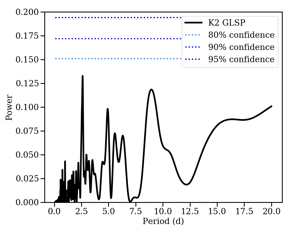
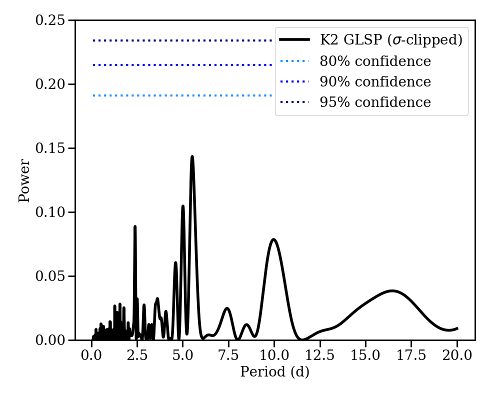
Figure 3: Top: GLSP for the complete K2 dataset. Bottom: GLSP for the $\sigma$-clipped dataset (out-of-eclipse data). The significance levels are estimated according to a red-noise model with correlation parameter $\alpha$=0.98 and the same uncertainty distribution and sampling as observed in the data (see text), so that the observed peaks are not significant.

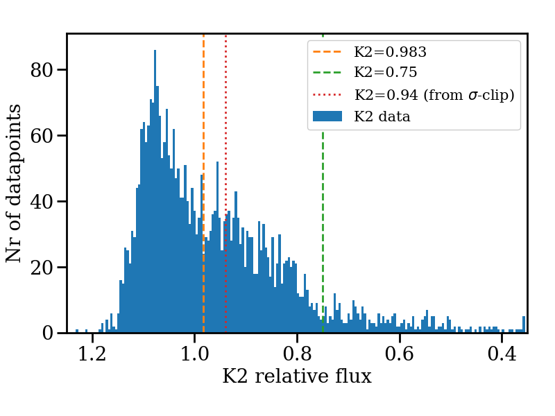
Figure 4: Histogram of the K2 data by magnitude. Note that there is no clear separation between the ”on-eclipse” and ”off-eclipse” parts, except for very deep eclipses (relative flux$<$0.75, green line). The red dotted line marks the separation from the $\sigma$-clipping filter. Selecting down to a different level (e.g. 0.983, orange line, where the distribution appears to slightly flatten out) does not introduce any significant change.

3.1 Periodicity analysis

A period of about 5d (albeit very uncertain) has been suggested as the rotational period of RX J1604.3-2130A from K2 data (Ansdell et al., 2016; Rebull et al., 2018). Here we revisit the periodicity in the K2 lightcurve to examine whether it is most likely due to rotation, or related to the obscuration events. The lightcurve is extremely irregular, suggesting variations in both the phase, the period, and the amplitude of the modulations and the presence of correlated, non-Gaussian noise. Therefore, we take two approaches to search for periodical signatures: generalized Lomb-Scargle periodograms (GLSP; Scargle, 1982; Horne & Baliunas, 1986; Zechmeister, & Kürster, 2009) and wavelet analysis (Torrence, & Compo, 1998; Liu et al., 2007).

Simple GLSP fail when applied to quasi-periods, so for the first approach we use stacked GLSP (SGLSP; Mortier & Collier Cameron, 2017), where the data are filtered around each single date to study periodicity only over a limited number of days. Repeating the exercise over time, changes in the period and phase can be tracked. Since the data distribution is highly non-Gaussian and strongly correlated, a red noise model is needed to assess the significance of the signatures. The red noise model was derived from the correlation between consecutive datapoints, parameterized by $\alpha$, the slope of the correlation between one datapoint and the next. For K2 data, we find $\alpha$=0.98. We then simulated data following a similar distribution where each value depends on the previous one (as given by $\alpha$) plus an stochastic component with values drawn from random numbers following the standard deviation of the observed data. For each K2 (S)GLSP, we computed 1000 red-noise simulations with the same number of datapoints, the same sampling rate, and the same red-noise model but without any periodic signature and used their periodograms to derive the confidence intervals.

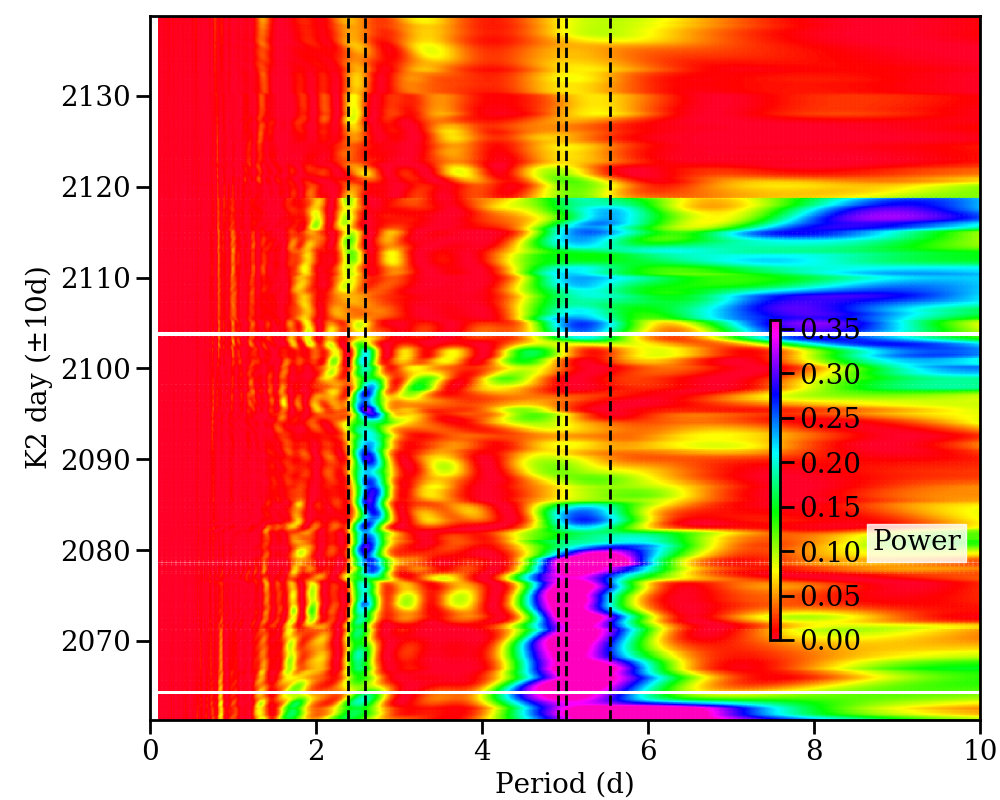
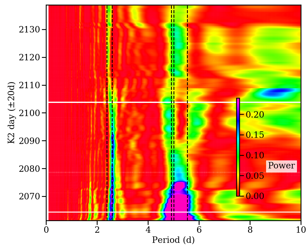
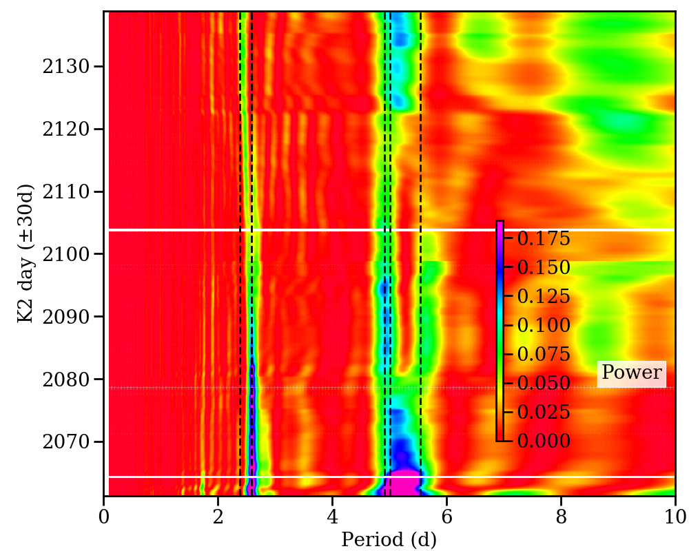
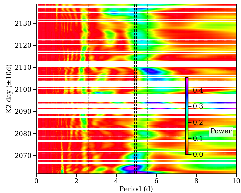
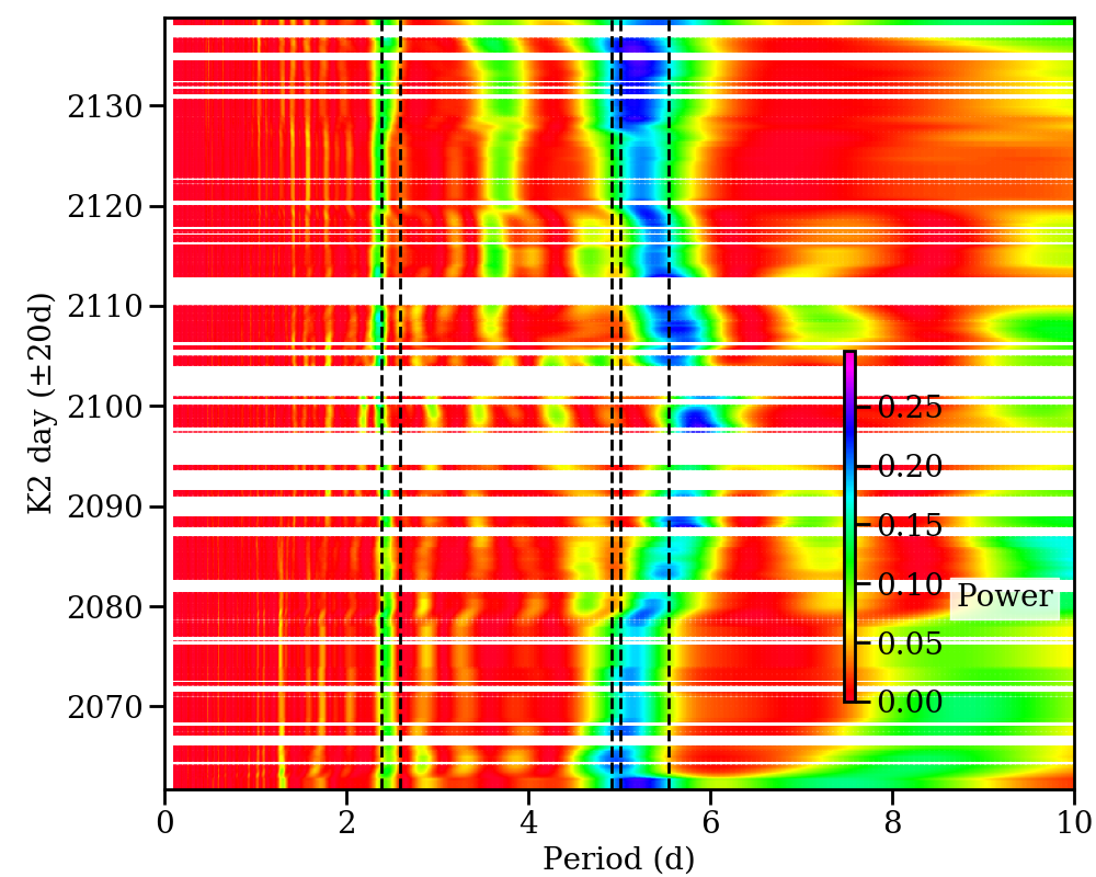
Figure 5: Stacked GLSP for the full K2 data (top three panels, stacking at intervals of $\pm$10d, $\pm$20d, $\pm$30d) and the $\sigma$-clipped data (out-of-eclipse data; bottom two panels, stacking at intervals of $\pm$10d and $\pm$20d). The most significant periods detected in the individual GLSP are marked with vertical lines (see text for discussion). In each panel, the x axis shows the periods and the y axis shows the date (in K2 mission days) around which we consider the time interval to estimate the SGLSP. Dates for which no data are available are left blank. The color scale is set such that purple is equivalent to 95% significance and dark blue is equivalent to 90% significance for a red-noise model with the same number of points, similarly distributed (see text).

A GLSP including all the available data suggests some signals with periods 2.5d (which could correspond to half the 5d period), 5d, and 9d, but none of them is highly significant (see Figure 3). The 5d periodic signature is reported in the literature as a rotational period, so we first examined the data belonging to the out-of-eclipse phase and the data belonging to the eclipses separately. Defining the ”out-of-eclipse phase” is not easy in a lightcurve that does not show a clear difference between the ”in-eclipse” vs ”off-eclipse” parts (see Figure 4). We thus cleaned the data using a $\sigma$-clipping algorithm to calculate the mean and standard deviation, and then removed all points that are beyond 3$\sigma$ from this value. The analysis of the off-eclipse data revealed that the periodic signatures are stronger when the full dataset is considered, and thus the (quasi-)periodicity is strongly linked to the eclipses, and not only to rotation.

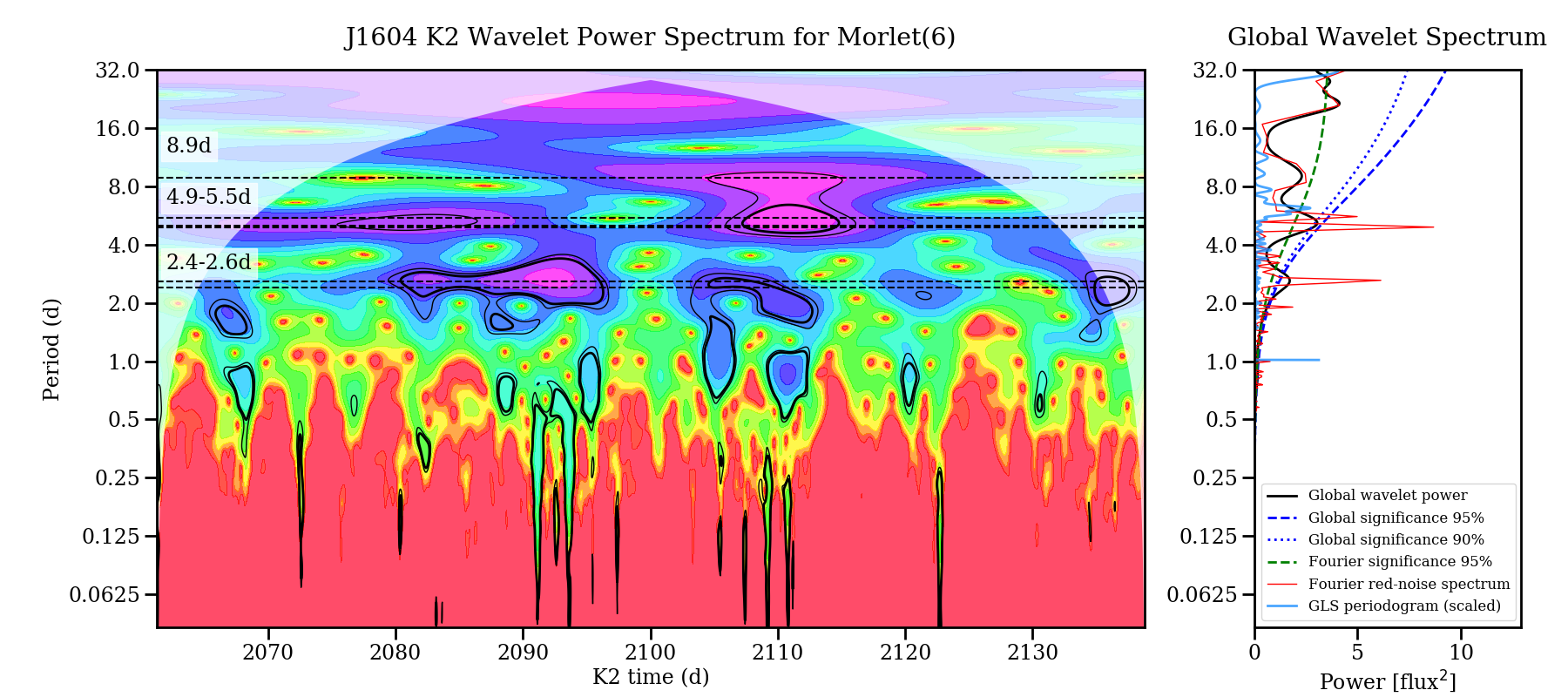
Figure 6: Wavelet power spectrum for the K2 data on RX J1604.3-2130. The left panel shows the wavelet spectrum in time. The color scale is set between minimum and maximum power, and the global significance limits are marked as thick black (95% confidence) and thin black (90% confidence) contours, calculated for a red noise data model with $\alpha$=0.98. The regions where edge effects could be significant are masked out. Horizontal lines mark the positions of the GLSP peaks found with K2 and REM (at 8.9d, 5.5d, 5.0d, 4.9d, 2.59d, 2.39d). The right panel shows the global wavelet power together with the significance, the noise spectrum, and the scaled GLSP for comparison.

We then stacked the data for different numbers of days around each point, and calculated SGLSP in intervals of $\pm$10d, $\pm$20d, $\pm$30d, and $\pm$40d. The number of days was selected to be large enough to detect the potential periods observed in the full collection of data, up to the limit of $\pm$40d that includes essentially the whole dataset and tends to the full-data GLSP. Figure 5 displays the results. The data reveals a 5d period in the stacked $\pm$10d and $\pm$20d diagrams, which progressively dilutes when more data are added. The period is not always present, and the peak changes between 4.8-5.5d, which makes it more plausibly a quasi-period related to a rapidly variable phenomenon than a typical rotational period, even if both may be connected. The 2.5d period is also present, although it has a lower significance except during the time of increased eclipse activity (approximately, from mission day 2085 to 2105), when eclipses occur at a higher rate. The 9d period is very broad and not well-defined.

For the second periodicity estimate, we use wavelet analysis based on a Morlet function with $\omega_{0}$=6, which typically offers the best results for complex datasets (Torrence, & Compo, 1998). The Morlet wavelet $\Psi$($\eta$) (Grinsted et al., 2004) is very similar to a sinusoidal function tappered by a Gaussian, written as

$$\Psi(\eta)=\frac{e^{i\omega_{0}\eta}}{\pi^{1/4}}e^{-\eta^{2}/2}.$$ (1)

Here, the time dependency is wrapped in the dimensionless parameter $\eta$, which takes values that are multiple of powers of 2 assigned through the dimensionless time series. In essence, the SGLSP and wavelet analysis are quite similar, with the main difference being that SGLSP uses a square passband to filter the data around a certain date, plus a collection of sinusoidal functions, while for wavelet analysis the wavelet functions (Eq. 1) play the role both the filter and the (complex) periodic function.

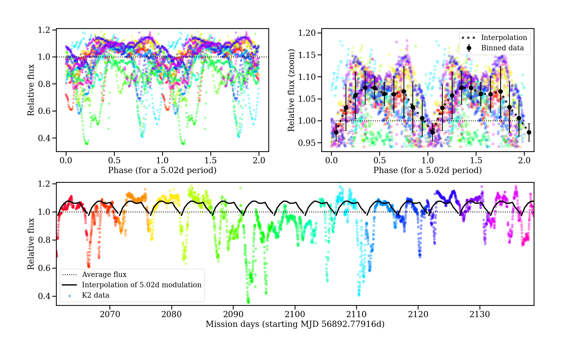
Figure 7: K2 data wrapped according to a period of 5.015d. The data are color-coded according to date to better display the points that were taken nearby in time. The upper left panel shows the entire K2 data wrapped, showing the phase twice to aid the eye. The upper right panel offers a zoom in the ”out-of-eclipse” part of the K2 data (colored points, selected via $\sigma$-clipping), together with the average and standard deviation in 10 intervals in phase space (black points; the errorbars correspond to the standard deviation within each bin) and an interpolation curve to trace the shape of the variations. The bottom panel contains the full K2 data plotted against mission day together with the interpolated modulation curve of the top-right panel, to show how the phase of the eclipses drifts at certain times during the observation campaign, although the 5d periodicity remains visible throughout the full dataset.

The wavelet analysis was performed using the Python PyCWT spectral analysis module (based on Torrence, & Compo, 1998; Grinsted et al., 2004; Liu et al., 2007). The procedure requires the data to be uniformly sampled, which is the case for K2 observations. The few small gaps and inhomogeneities in the data were filled by interpolation. While this may have an effect on the shortest timescales sampled, it does not affect the final significant periods, which are in the range of days. The significance was estimated considering a model for red noise estimated through a Lag-1 autocorrelation of the original data (Torrence, & Compo, 1998; Liu et al., 2007). The results of the wavelet analysis are plotted in Figure 6. The wavelet analysis recovers the results of the SGLSP and shows the same trends of quasi-periodicity, with significant signatures in the range of 2.4-2.6d, 4.9-5.5d, and, to a lesser extent, 9d. As for the SGLSP analysis, not all the periods are recovered on all epochs and there is a drift in phase and periodicity that suggests changes in the structure that causes the eclipses.

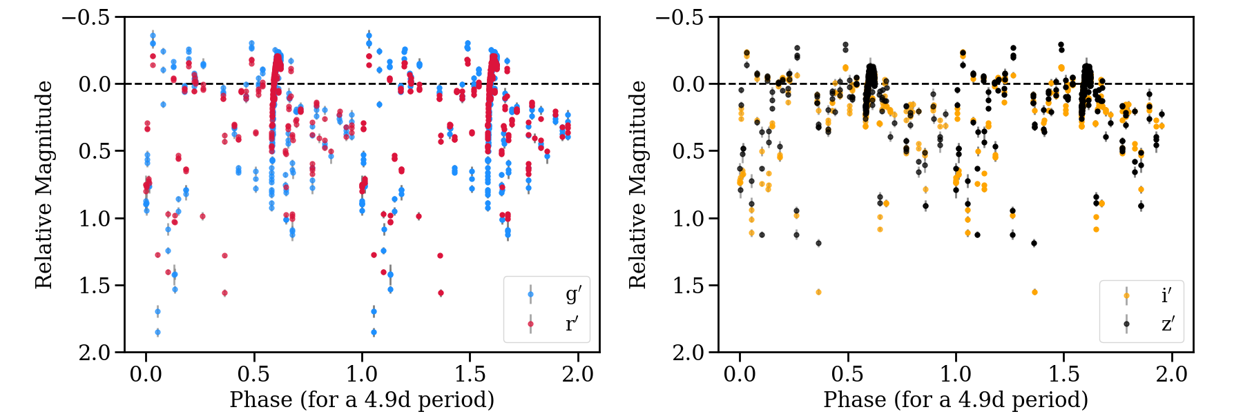
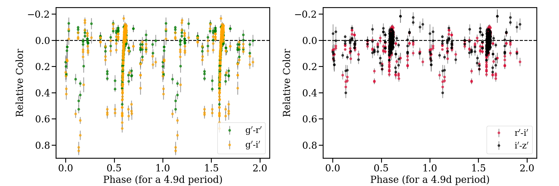
Figure 8: Top panels: REM data, wrapped for a 4.9d period to reveal the presence of periodic signatures. Bottom panels: REM colors, wrapped for a 4.9d period. All the magnitudes are given relative to the median magnitudes in each filter.

To help visualizing the periodicity, we phase-wrapped the data for the various potential periods. This exercise reveals a clear modulation for a period of 5.02$\pm$0.12 d (corresponding to the main peak of the GLSP, see Figure 7) and, to a lesser extent, for a period of half this value. Any other period fails the visual check or appears to be spurious (e.g. being an integer multiple of the sampling rate). The overall shape of the curve suggests a 5d quasi-periodicity for the eclipses, and at the same time reveals a clear but rapidly changing modulation in the flux observed out of eclipse. The tip of the phased lightcurve has a ”M” shape that could be consistent with rotational modulation in a star with two non-identical cold spots (see Figure 7 top right). Nevertheless, we also observe that the modulation suffers significant changes from one period to the next, which is unfeasible for typical long-lived, cold stellar spots. The eclipses are clearly associated to this 5d period, although they also change in depth from period to period and show a drift in phase during the observed epochs (Figure 7 bottom). The epochs of increased eclipse activity correspond to the times when the 2.5d period is stronger. Having ruled out relatively stable structures (e.g. spots) for the variability, the observed lightcurve requires something that changes on the timescale of the rotational period, such as significant variations in the obscuring material in the innermost disk. The various possibilities will be discussed in the following sections.

The REM data do not offer the same kind of time coverage and photometric stability, and thus the periodicity that can be inferred from them has low-significance. Moreover, the correlated errors in the REM magnitude are very complex as the ”redness” of the noise strongly depends on the observed cadence and the magnitude (given the typical cadence, it is unlikely to find many consecutive points on eclipse so that low magnitudes tend to be followed by quite uncorrelated ones, while ”out-of-eclipse” points are often followed by a measurement with very similar value). This makes it very hard to assess the significance of the GLSP and makes a wavelet analysis impossible. Nevertheless, the same rough behavior is observed, and wrapping the lightcurve reveals a dominant periodicity around 4.9d that appears correlated with the extinction events (see Figure 8). There is no high-cadence periodic signature.

3.2 REM data, extinction, and the inner disk structure

The multi-band REM data allows us to study the color variation during the eclipses for the first time. The JHK data could provide a good insight about the properties of the obscuring matter, but the only dates for which we have complete data do not reveal substantial variability, and the only filter for which we cover a significant number of points and shows variability is H. The optical data taken around the same dates as JK reveal that the object was essentially out of eclipse. The observed JHK colors are consistent with the colors of a pre-main-sequence star without significant near-IR excess (Kenyon & Hartmann, 1995).

We thus concentrate on examining the optical and H-band data. Figure 9 shows the color variation as a function of the magnitude variation for several combinations of bands. Considering the standard interstellar extinction laws (R_V=3.1-5.5, see for instance Schlegel et al., 1998; Stoughton et al., 2002; Cardelli et al., 1989), the slopes of the color variations up to $\Delta$g’$\sim$1 mag are quite consistent with the standard extinction vectors. There are some places where the color variation becomes suddenly smaller, for instance around $\Delta$g’$\sim$1 mag and (especially in the g’ vs r’$-$z’ diagram), around $\Delta$g’$\sim$0.2 mag. These could be due to scattering shifting the colors towards bluer regions as the eclipse progresses (as has been observed in UXors, e.g. Grinin, 1988). There are further changes in the slope as the eclipse progresses, with the deeper eclipses being better fitted with an extinction law with higher R_V (which is in general attributed to high extinction clouds with more processed material; Cardelli et al., 1989) and the very deep eclipses having an offset with respect to the standard trend and showing a flatter reddening curve.

The color variation towards flatter reddening curves is only observed for eclipses with $\Delta$g’$\sim$0.9-1.1 mag. In those cases, the reddening continues into the deepest eclipses (for which $\Delta$g’$\geq$0.9) with a slope that cannot be explained with the standard R_V=3.1-5.5. The slope variation is likely related to strongly processed dust grains, although the change is different in different filters, maybe indicating an effect of grain size (Eiroa et al., 2002). Higher density or differences in dust properties and/or scattering within the clumpy material of the disk could also contribute.

There are also some shifts parallel to the extinction vectors visible at about all magnitudes. Small variations in the stellar luminosity (e.g. due to accretion) and/or scattering on longer timescales may also contribute to shift some of the data taken on different dates parallel to the standard extinction vectors as seen in Figure 9, even though small stellar luminosity and accretion changes are not expected to produce a significant change in the observed colors. Note that a large fraction of the shallower eclipse points belong to the high-cadence observations and thus were taken very close in time, so that their variation is smooth.

Leaving aside the UXor behavior towards bluer color, the changes in the color slope consistent with reddening could be caused by extinction by more opaque material in the deepest parts of the eclipse and variations in the sizes of the grains depending on the height in the innermost disk (e.g. McGinnis et al., 2015), due for instance to differential settling (e.g. D’Alessio et al., 2006; Laibe et al., 2014). The dust content around a star is constrained by the dust sublimation temperature ($\sim$1500 K, with some variations in the 1000-2000 K range depending on disk structure, density, and composition; Isella & Natta, 2005; Kama et al., 2009), and typical observations can be well-fitted with inner rims at T=800-1200 K (McClure et al., 2013). Significant grain processing happens already at these (and much lower) temperatures (Tielens et al., 2005), so that the grains are likely different from plain ISM silicates. Grain growth is also generalized in disks, and larger grains tend to produce grey extinction with a lower color dependency at optical and near-IR bands (Miyake & Nakagawa, 1993; Eiroa et al., 2002), and large grains are often involved in the best-fitting models for inner disk walls (McClure et al., 2013). In addition, there are other effects such as a dusty wind (e.g. as observed in RW Aur; Bozhinova et al., 2016) that could also cause obscurations. The H$\alpha$ profile of RX J1604.3-2130A shows some blueshifted absorption (Manara et al. in prep., see also Section 3.3), but since the accretion rate is low, accretion-related winds are expected to be weak and carry significantly less mass than the accretion flows.

The high-cadence data offers us a chance to explore what happens during a single eclipse on a timescale where the variations (accretion, luminosity) are likely negligible (Figure 11). The data show a smooth transition from eclipse to maximum, although the high-cadence eclipse does not go as deep as those where a significant color offset is observed. The high-cadence data are fully consistent with a mild UXor behavior around $\Delta$g’$\sim$0.2 mag, plus increasing dust extinction with standard extinction laws for thin ISM dust (R_V=3.3). For the rest of the eclipses, including those happening at half of the period, the coverage is very scarce, but wrapping the data does not reveal a significant difference between the colors of different eclipses, nor between the colors of the full-period vs half-period eclipses (see Figure 8 bottom), other than the differences observed between shallow and deep eclipses.

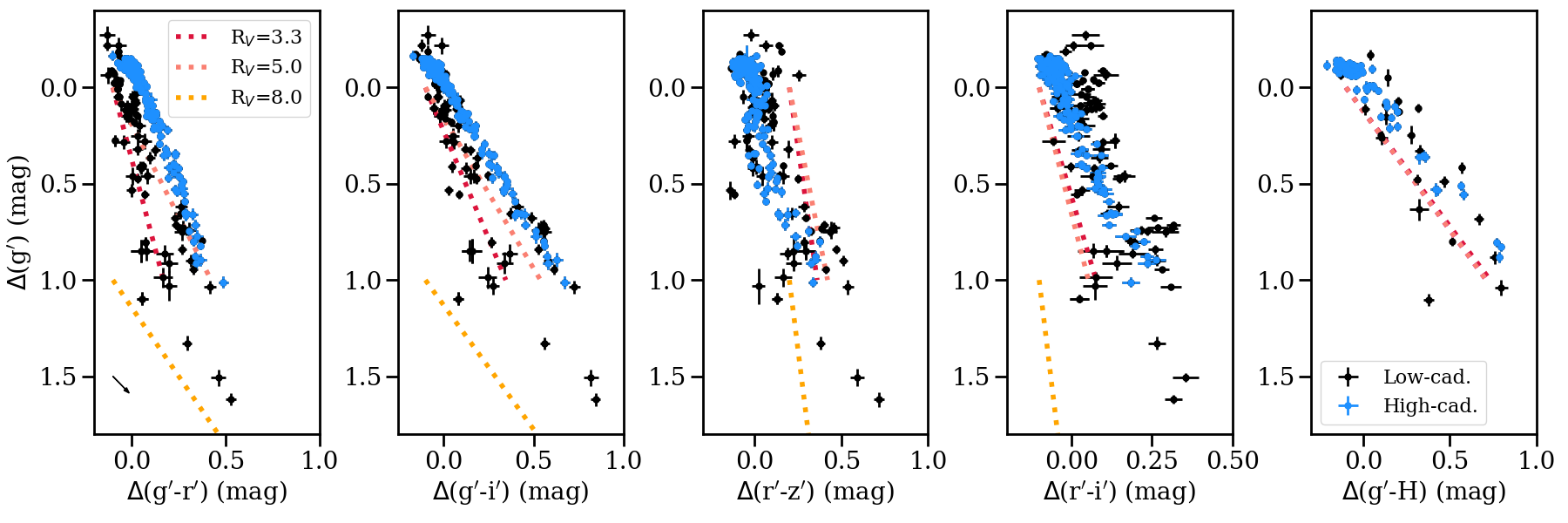
Figure 9: Relative color-magnitude variations in the optical and H-band REM data. The dotted lines indicate the extinction vector for several extinction laws (R_V=3.3,5.0 and 8.0, derived following Schlegel et al., 1998). High-cadence data are plotted in blue, while the rest of data are shown in black. All magnitudes are relative to the median value in each filters. The black arrow in the left of the first panel shows the correlation direction for cases where g’ is also used to calculate the color, showing 3$\times$ the average uncertainty.

We can then use the observed extinction to estimate the amount of material needed to produce the eclipses. The typical depth of the extinction event in g’ is 1.2 mag. Assuming standard interstellar extinction (Schlegel et al., 1998), this is equivalent to A_V=1 mag, or N_H=1.8e21 cm^-2 (Predehl & Schmitt, 1995). For an average particle weight of 1.36 m_H (for solar metallicity neutral gas, e.g. see Mihalas, 1978), we obtain 0.004 g cm^-2. Note that because the metal vs hydrogen content in the inner disk may be different (either higher or lower, e.g. Panić et al., 2009; Riviere-Marichalar et al., 2013), there is some uncertainty in this parameter. The stellar parameters suggest a dust destruction radius at 0.06-0.15 au. If this mass were distributed in a ring of radius 0.06 au (0.15 au) and height comparable to the stellar radius, the total mass associated to the structure would be about 2e-3 (5e-3) M_Ceres, including gas and dust. Nevertheless, we can derive a better estimate of the thickness of the structure from the observed shadows in the outer disk, that span about 20 deg in average (see sketch in Figure 10). For an obscuring structure at 0.06 au (0.15 au) distance, this would mean a size about 0.02 au (0.05 au) or 3R_∗ (8R_∗) as a function of the stellar radius. The total as plus dust mass would be in the range 1-6% of the mass of Ceres. This means that the innermost disk ring does not need to be very massive in order to reproduce the observed behavior. An extinction law for dark nebulae would result in a slightly larger mass, although for reasonable values the main uncertainty in our estimate remains the uncertainty in the size of the innermost disk and the gas to dust ratio.

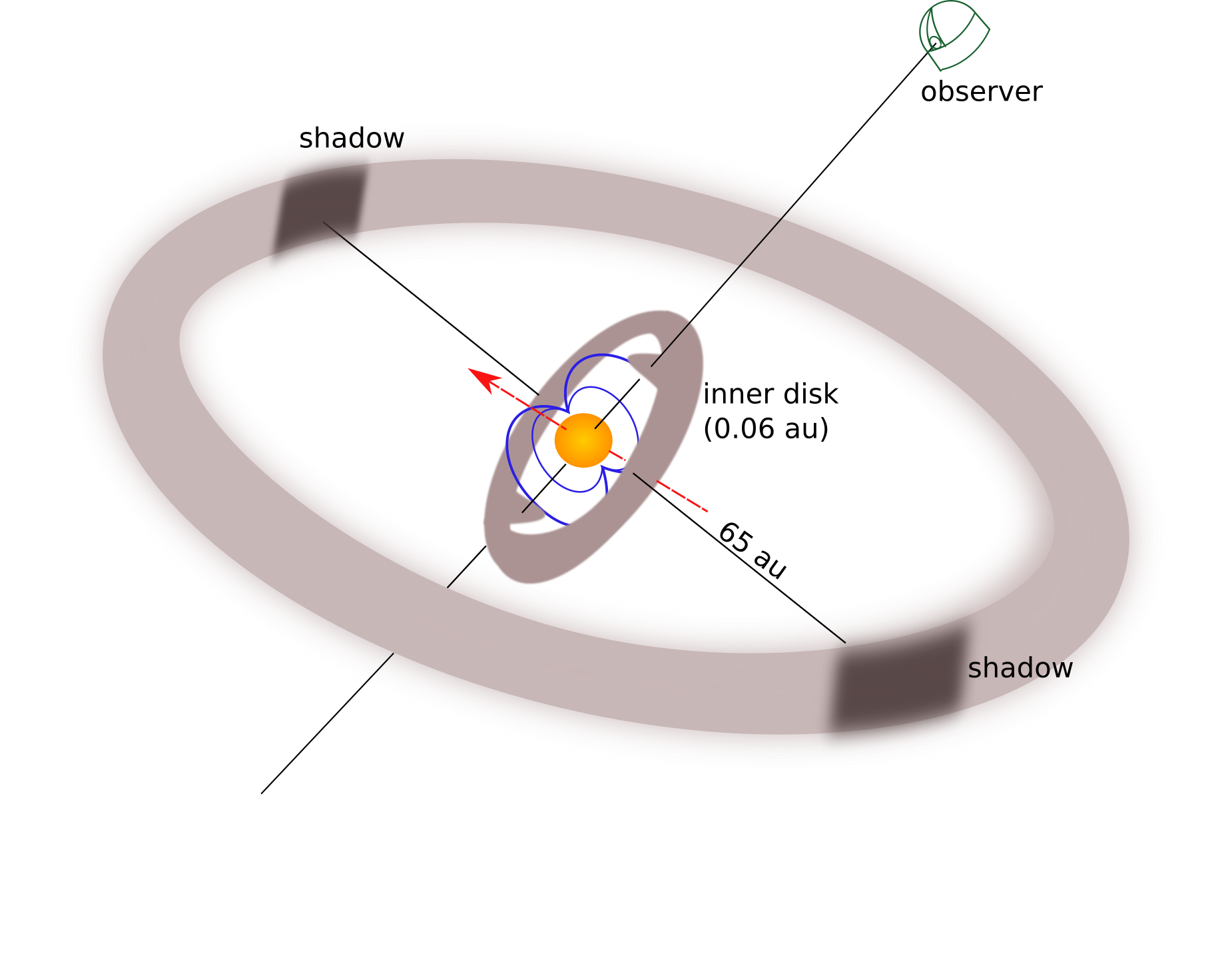
Figure 10: Not-to-scale sketch showing the inferred structure of the system. The star and its magnetosphere are displayed in the center, the red arrow indicates the rotation axis of the star, magnetosphere, and corotating inner disk. The inner disk is deformed in the regions where the magnetosphere is joining in, which causes warps that cross our line-of-sight when the disk rotates. The outer and inner disk are highly inclined with respect to each other, so that there are always shadows along the line where the plane of the inner disk and the plane of the outer disk cross. Note that the inner disk is expected to be more wobbly and irregular than shown here.

Pinilla et al. (2018) revealed flux variations in the scattered light J-band observations up to 0.4-0.6 with respect to the non-obscured flux. Standard extinction laws suggest A${}_{g}\sim$2.6-4.3 mag, about a factor of 1.4-2.3 higher than in the deepest optical eclipses, which would result in a similarly larger mass. There are several possibilities to explain this difference. Differences in alignment between the star-inner disk and the inner disk-outer disk could result in different column densities viewed on each line of sight (see Figure 10). In addition, the fact that the shadow observations and the optical photometry are not simultaneous and the dust content is known to be variable, plus the possibility that the dust does not follow a standard extinction law, especially in the deepest eclipses, may also play a role. Other possibility would be if the inner disk does not cover the full stellar disk along our line-of-sight, or if the disk does not generally covers the surface of the star but a localized warp or blob on it does. In fact, the observed differences in extinction (observed from the lightcurve A${}_{g}\sim$0.4–1.8 mag, expected from shadows A${}_{g}\sim$2.6-4.3 mag) can be explained with a variable stellar disk coverage by the eclipsing material. Considering the density estimated from the extinction a variation in coverage ranging from 0% out of eclipse, to between 30% for shallow eclipses, down to 100% at the deepest ones could explain the observed lightcurve. Note that the optical variability depends on various poorly-constrained parameters, such as the relation between infrared and optical extinction (i.e., dust properties), whether the disk is occulting the star towards the equator or towards the poles (due to limb darkening), and whether the star has additional causes of variability (e.g. hot and cold spots).

The observed small changes and displacements of the shadows are consistent with a ”wavy” or warped disk (Pinilla et al., 2018), which is also consistent with other observations (Grinin et al., 2008; McGinnis et al., 2015), models of self-shadowed UXor disks (Dullemond et al., 2003), and the non-axisymmetric or clumpy structures observed in gas and dust in the inner disks of some young stars (e.g. Sicilia-Aguilar et al., 2012; Siwak et al., 2014; Scholz et al., 2019). A warp at the point where the disk and the star are connected at the basis of the accretion column (see e.g. the models of Alencar et al., 2012, 2018; McGinnis et al., 2015; Bodman et al., 2017) could also explain the observations, as shown in the cartoon in Figure 10. The variations of the position of the shadows ($\sim$20 deg in average; Pinilla et al., 2018) together with the estimated radius of the disk suggest that the innermost disk is as wavy as it is thick. A wavy/warped disk that deviates from a flat structure in vertical scale by about a third of the disk radius (to account for the angle variation of the shadows) would also explain why the star is not always eclipsed, while the shadows on the outer disk are nearly ubiquitous despite variability.

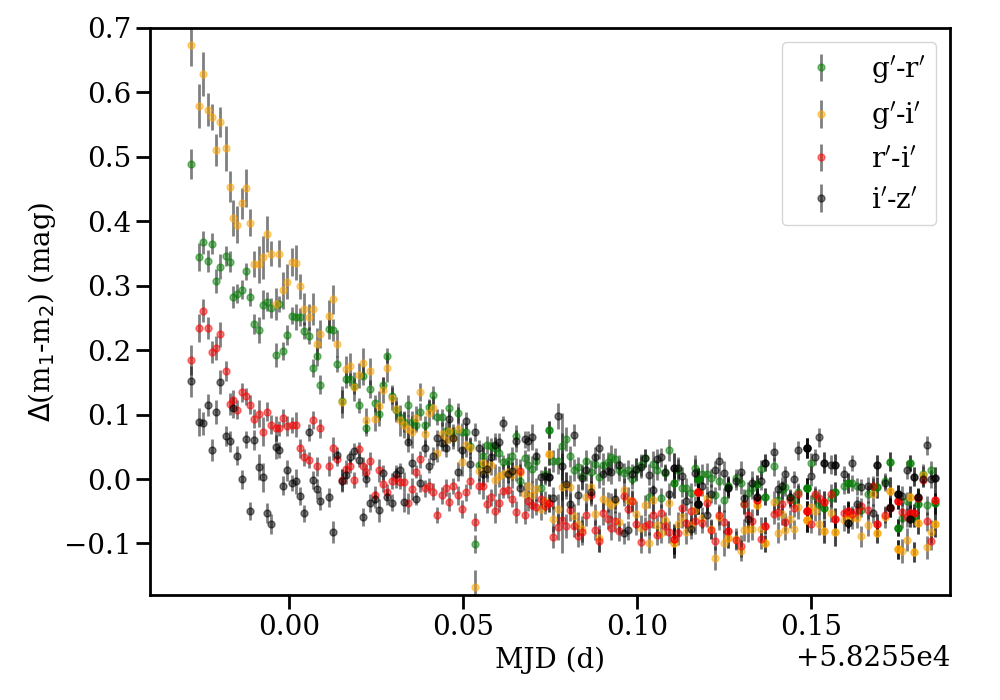
Figure 11: Color variations in the dip observed with the high-cadence data. Note that the eclipse is not deep enough to show significant variations in the extinction law, although some of the UXor behavior is seen, especially in i’-z’.

A 5d orbital period corresponds roughly to the distance where the disk would have a temperature around 1540 K ($\sim$0.06 au or 9.4 R_∗). The precise location and temperature depend strongly on the dust properties, on the structure of the inner disk rim, and on the stellar parameters (especially, the stellar mass derived from evolutionary tracks). But in any case, the corotation radius is compatible with the dust sublimation radius. With this in mind, the quasi-periodicity of the eclipses discussed before suggests that the structure causing them is rapidly changing on timescales comparable to the Keplerian period of the material in the innermost disk (days), so that even consecutive eclipses have different depths and lightcurve profiles. Disk precession may alter the inclination of the inner disk in time, but their timescales are typically much longer. For the general relativistic precession, the timescale is proportional to $(c/v_{K})^{2}$ times the orbital period, where c is the speed of light and $v_{K}$ is the Keplerian orbital velocity. Kozai or secular resonances may also cause precession, but they are usually weaker than the relativistic effect (Kozai, 1962; Ford et al., 2000) and require very massive and close-in companions that would have been spectroscopically detected .

The quasiperiodicity on short timescales and color variations suggest that the disk is highly asymmetric, with warps or clumps that are denser than the rest. It is also likely being externally modified/fed due to viscous matter transport, which can explain the sudden periods of intense dimming and concatenated eclipses, such as the one observed between days 2085 and 2105 in the K2 data (see Figure 2). Taking into account the accretion rate $\sim$3e-11 M_⊙/yr and assuming that the rate of transport of matter in the inner disk is similar, the mass of the innermost disk required by the eclipses is comparable to what accretion transport could provide in between two weeks to two months time. This means that the inner disk is filling up (and draining) on relatively short timescales, so that significant changes could be observed on 5d timescales.

To summarize this section, the color variability confirms that the eclipses are consistent with extinction by dust with properties ranging from ISM dust to more processed grains, located in an irregular, warped disk at the corotation radius. The total mass depends on the dust properties and on the size of the disk, but $\sim$1% M_Ceres of total mass (including gas and dust) is enough to explain the observations. Considering the accretion rate, it is not unexpected that the dust distribution in the innermost disk changes on short timescales, since a significant fraction of the obscuring matter in the innermost disk will be fed to the star (or drained from the innermost disk) on each rotational period, explaining the rapid variability.

3.3 Rotation, accretion, and variability in the inner disk

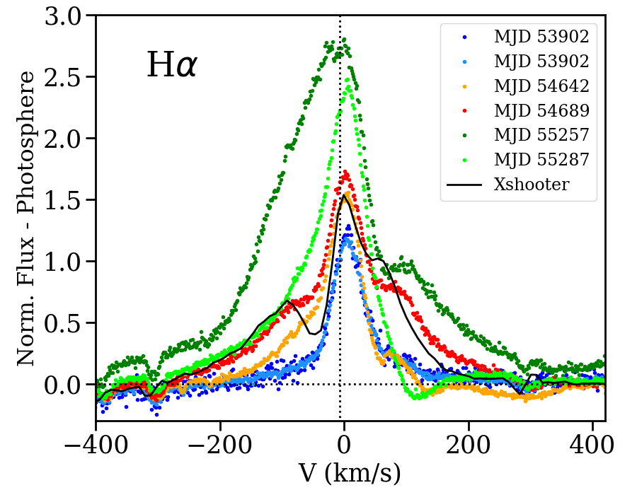
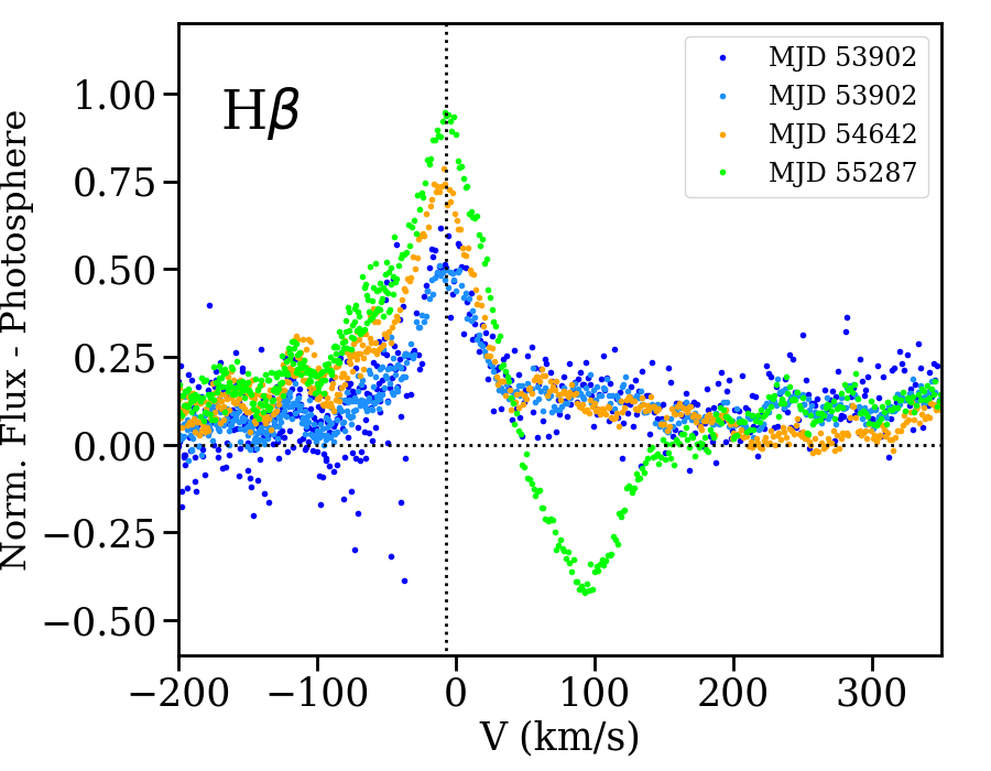
Figure 12: Photosphere-subtracted H$\alpha$ (top) and H$\beta$ (bottom) spectra observed with HIRES/Keck (for various epochs) and X-Shooter (corresponding to the time when the accretion rate and the stellar properties were estimated; Manara et al. in prep). The zero level for flux and radial velocity are marked by dotted lines. A rotationally-broadened template photosphere has been subtracted to show the absorption and emission features.

Rotation rates suggested a very high inclination for the disk system around RX J1604.3-2130A (Davies, 2019), despite its outer disk being nearly face-on (6 deg; Zhang et al., 2014; Dong et al., 2017). If the 5d modulation observed was caused by rotation, we can use the observed rotational velocity (16.2$\pm$0.6 km/s) to infer the inclination of the system. The maximum period that this velocity range allows is 4.2-4.5d. A 5d period would require a stellar radius $\sim$10-15% larger than estimated, or larger uncertainties in the v$sini$ (e.g. due to differences in limb darkening). In any case, the star cannot be aligned with the outer disk because it would rotate at breakup velocity, but should be closer to equator-on and thus rather aligned with the inner disk. If the 2.4-2.5 d period were a rotation period, the inclination angle would be about 38 degrees (still far from aligned with the outer disk). Nevertheless, such a low angle would be inconsistent with the lower limit of 61 degrees of Davies (2019), besides the fact that the shape of the lightcurve agrees rather with a 5d rotational period in a star with two asymmetric eclipsing structures, rather than with a 2.5d period.

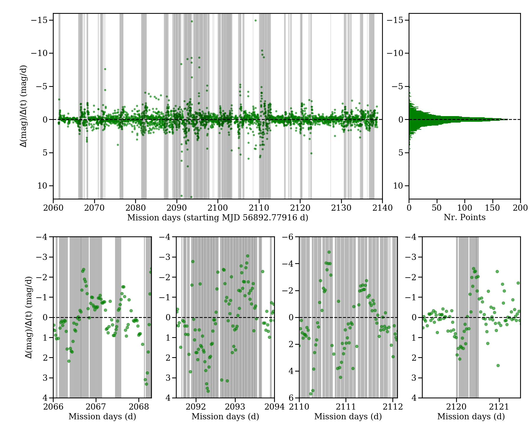
Figure 13: Time variation for the K2 observations. The upper left panel shows the change in magnitude per day as a function of the observing date Grey lines mark the cases in which the K2 relative flux drops below 0.94 (the limiting value for eclipses considered, see text). The upper right panel is a histogram of the same plot. The lower panels are a zoom-in of the magnitude change vs time for several of the eclipses.

Constructing a model for the out-of-eclipse lightcurve is complicated, because the sampling of the REM photometry is not high enough to show the detailed color variation during a single rotational period and there are significant changes on a few-days basis (see Figure 8). A cold spot model is not sufficient since spot-related variability is usually of the order of 0.1 mag (Grankin et al., 2007) and can by no means explain the observed eclipses nor shadows, but it could explain the M-shaped part of the K2 data. The flux modulation at phase $\sim$0.5 (see Figure 7) can be obtained with spots 200-500 K cooler than the stellar photosphere and spot coverage between 0.03 and 0.36 (as in e.g. Bozhinova et al., 2016), all of them reasonable parameters, but the rapid variability from period to period is hard to explain. For instance, a smaller-scale eclipse could also produce the same effect, and since the amount of matter responsible for this would be very small compared to what is observed to flow around the star from its accretion rate, rapid variations are more plausible. In addition, there is more evidence of the disk-star connection being dynamic and rapidly variable than in the case of stellar spots (e.g. Fonseca et al., 2014), and the color variations (Figures 8, 9, and 11) suggest that occultations are the dominant process.

All the datasets (CSS, K2, and REM) show brief periods of increased eclipsing activity on timescales shorter than 5d (usually, about 2.5d). These could be times at which an increased accretion rate throughout the disk triggers accretion onto the other side of the star and feeds a secondary warp, causing additional extinction events. Modeling this situation would require, at a minimum, simultaneous high-cadence multi-color photometry and spectroscopy and it is thus beyond the scope of this paper.

The archival HIRES data are consistent with the low accretion rate estimates from X-Shooter spectra (Manara et al. in prep), not showing the emission lines characteristic of strong accretors (Hamann & Persson, 1992, for instance, no He I emission and Ca II IR narrow emission lines in the center of strong absorption components). There is also no evidence of spectroscopic binarity (see Appendix C). H$\alpha$ and H$\beta$ have strongly variable intensity and line profiles, with timescales of months to years. The features are better viewed after photospheric subtraction, using a photospheric template derived from the standards HD 114386 (which has been observed in the H$\beta$ region) and HD 151541 (for which the available data covers the H$\alpha$ region; see Figure 12). After photospheric subtraction, H$\beta$ emission becomes evident, together with evidence of both redshifted and (in H$\alpha$) blueshifted absorption components. Photospheric subtraction also reveal further complex absorption profiles in other lines, such as Na I D. Since there is no detailed day-to-day high-resolution spectroscopic followup, it is hard to assess whether the variations in the line profile are due to variations in the accretion rate or changes in the orientation of the accretion flows with respect to the observer. Nevertheless, the changes in equivalent width and 10% velocities suggest that the accretion rate is variable, with up to 2 orders of magnitude variability between the maximum and the minimum width (using the 10% H$\alpha$ width; Natta et al., 2004), with the 3e-11 M_⊙/yr value from Manara et al. in prep. being an intermediate rate. Accretion is very weak (consistent with no accretion) in the spectra from MJD 53902.

For both the H$\alpha$ and H$\beta$ lines, the redshifted absorption features are dominant, and on two of the dates (MJD 54642 and MJD 55287) show a YY Ori or inverse PCygni profile (IPC) with an absorption component that goes below the continuum. This suggests that the accretion column must have been very close to viewed along the line-of-sight on these dates. Accreting along the line-of-sight could also mean that the gaseous material could be also obscuring the star (as has been suggested in other objects, e.g. TW Hya; Siwak et al., 2014). Obscuration by dust could happen in a warp induced in the place where the accretion column is attached to the disk (McGinnis et al., 2015; Alencar et al., 2018) although unfortunately none of the spectra has simultaneous photometry. The spectrum taken on MJD 54642, which shows a mild IPC profile in H$\alpha$, is the one closest to a photometric datapoint from CSS corresponding to a deep eclipse. However, the HIRES data were taken 24h after the photometry, and since typical eclipses last less than 24h, it is not possible to assume that the star would have been in eclipse. Moreover, phase shifts are expected between the very-close-in gas emitting H$\alpha$ and eclipses associated to dust at the corotation radius. On MJD 55287, the IPC is clearly visible in H$\alpha$ and very strong in H$\beta$, a typical signature of highly inclined system (Alencar et al., 2012, 2018; Donati et al., 2019). This, together with the observed eclipses, is a sign that RX J1604.3-2130A may be very similar to other highly-inclined systems such as Lk Ca15, AA Tau, and V354 Mon (Bouvier et al., 2007; Alencar et al., 2018; Donati et al., 2019; Fonseca et al., 2014).

Since the analysis of the extinction suggests an inner disk that is routinely drained on a short timescale due to accretion, we explore whether the rate at which the magnitude varies during the eclipse is consistent with material transported due to accretion. A change in magnitude vs time is equivalent to a change in column density over time, using the conversion between extinction and column density as in Section 3.2. Assuming that this extinction event covers the stellar surface uniformly, the obscuring mass involved per time can be obtained by multiplying by the area of the stellar disk. This value can be then transformed into a approximate ”projected” accretion rate that can be compared to the accretion rate measured by spectroscopy. Because the REM data has only very scarce coverage of each dip, we need to do the exercise with the K2 data, although one of the main limitations is the lack of color information.

For K2, we calculate the change in magnitude between each two points $i$ and $i+1$ using the flux ratio between these two points to estimate the variation in magnitude as $-2.5log_{10}(f_{i+1}/f_{i})$. Dividing by the time interval we can obtain the change in magnitude vs time (Figure 13) and transform it into an approximate accretion rate as explained above. Using the conversion between K2 extinction and A_V (A_V=0.4 A_K2; Rodrigues et al., 2014) we obtain a typical change of 1 mag/day. With the relation between A_V and column density (Predehl & Schmitt, 1995), we derive an approximate accretion rate of 6e-12 M_⊙/yr. The large majority (99.1%) of the observed points fall between the (-5,+5) mag/day interval, and these would correspond to accretion rates up to 3e-11M_⊙/yr, fully consistent with the accretion rate estimates from X-Shooter observations (Manara et al. in prep). Note that these ”changes” do not need to be accretion rate variations, since we are only taking into account matter along the line-of-sight, and that the estimates are also subject to the same uncertainties than the inner disk mass estimates, namely dust properties and gas to dust fraction. It is also important to keep in mind that the obscuring matter contains dust and must then be located at least at the dust destruction radius near the star-disk connection, while what is observed in H$\alpha$ corresponds to hot gas likely closer to the stellar photosphere. Because of this, changes in the dust are not expected to be observed as immediate changes in H$\alpha$, and a phase delay is very likely to occur, as it is also observed between accretion-related emission lines with different energetics (Sicilia-Aguilar et al., 2015), or between veiling and line emission, or optical and X-ray accretion signatures (Dupree et al., 2012).

3.4 The long-term variability of the inner disk

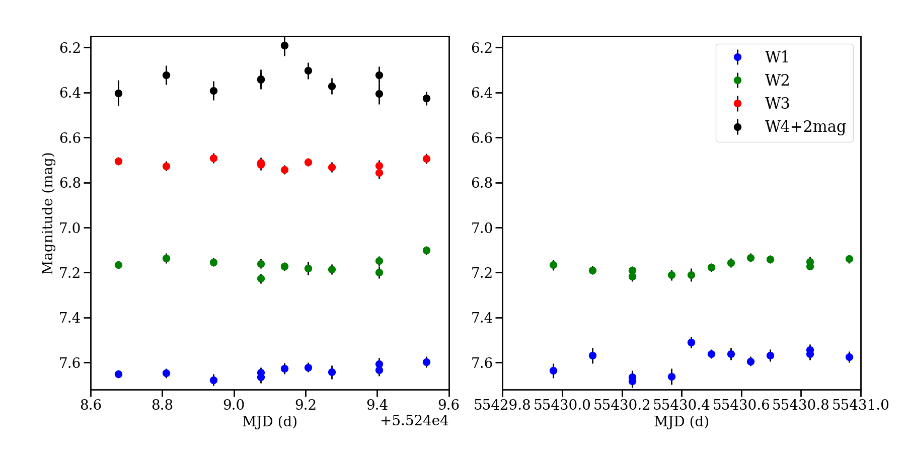
Figure 14: WISE lightcurve during the two periods of observation. The W4 magnitude, significantly brighter than the rest, has been shifted by 2 mags for display.

The disk around RX J1604.3-2130A has been classified as transitional (Carpenter et al., 2006; Mathews et al., 2012; Esplin et al., 2018). Luhman & Mamajek (2012) pointed out that the mid-IR observations with Spitzer/IRAC were consistent with a bare photosphere, while WISE data revealed a clear IR excess. Considering the fluxes provided by Carpenter et al. (2006) and the IRAC zeropoints, we find that the source changed by about 1.47 mag at 4.5$\mu$m between the Spitzer and the WISE observations, which are roughly separated by 4 years time (from MJD 53820 to MJD 55249). The AllWISE lightcurve, on the other hand, reveals only mild mid-IR variability (as expected if the cause is extinction) during the half a year interval during which RX J1604.3-2130A was observed by WISE (see Figure 14), with amplitudes of 0.17 mag (W1), 0.13 mag (W2), 0.07 mag (W3) and 0.24 mag (W4). It is interesting that while W1, W2 and W3 roughly follow the same pattern and vary in parallel, W4 behaves differently, although the uncertainties are also larger. At longer wavelengths, the extinction becomes negligible, so large changes in the flux are most likely related to changes in the disk structure. Wavelengths around 22$\mu$m trace material at considerably larger distances, and could be dominated by the emission of the outer disk, less variable on short timescales. Note that the dramatic ($>$1 mag) IR variability affects only the IRAC bands, since W4 and MIPS 24$\mu$m roughly agree despite being observed at times where there is substantial difference for the 3-10$\mu$m fluxes. Therefore, although the strong variability in the near-IR is reminiscent of the ”seesaw” behavior observed in some disks (e.g. Espaillat et al., 2011; Flaherty et al., 2012), we note that the situation here is quite different, because the mid-IR fluxes are not variable. While seesaw behavior in (usually, pre-transitional) disks can be explained by changes in the vertical scale without much modification to the contents of the disk, here the observed near-IR photospheric colors need a very strong depletion of warm dust.

The CSS data reveal decreased eclipse activity soon after the Spitzer observations were obtained, which points towards the intriguing possibility that the inner disk may have been depleted of dust around that date. The CSS data closer in time to the Spitzer observations (56 datapoints in total within 10-20 days) do not show any eclipse, although there are no observations for nearly half a year before the Spitzer observations and the first data point was taken more than 40 days after Spitzer. The sparse sampling may have missed the eclipses, since the CSS observations were obtained at irregular intervals of a few days during 2 months. However, with the sampling frequency and given that, altogether, 35% of the CSS observations appear to have been taken during eclipses, it is significant that not a single eclipse would have occurred near the time of the Spitzer observations, suggesting that the eclipse activity may have indeed been lower at the time. In addition, the HIRES spectra taken during the CSS stable phase after the Spitzer observations show a significantly weaker H$\alpha$ feature, consistent with decreased accretion and maybe an additional signature of lack of material in the innermost disk.

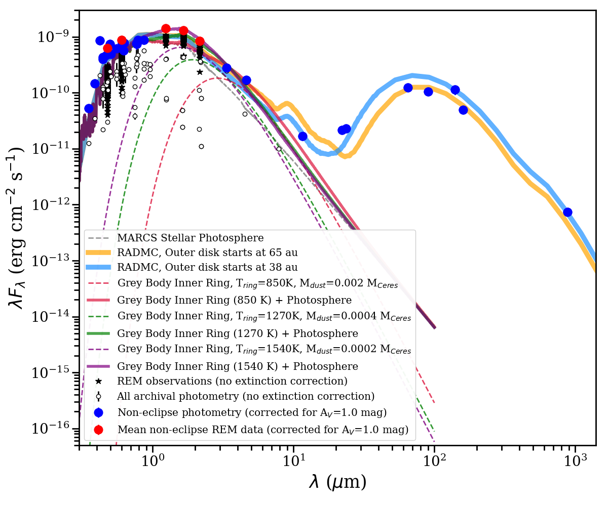
Figure 15: SED with archival data for RX J1604.3-2130A and simple disk models. The open dots show all the available data obtained from VizieR and not corrected for extinction. The REM data are shown for the filters with negligible color terms. The blue dots show the selected brightest magnitudes for each band, corrected by the nominal A_V=1.0 mag (Preibisch & Zinnecker, 1999). Three very simple models are shown for comparison for the purpose of estimating the mass that could be associated to inner disk emission (see text for details): Two constructed using RADMC radiative transfer code, and two assume a grey body model for material located in a ring with temperature 850 K and dust mass 0.003 M_Ceres, a temperature 1270 K, dust mass 4e-4M_Ceres, and a temperature of 1540 K with dust mass 2e-4M_Ceres, respectively.

The strong Spitzer vs WISE mid-IR variability is very similar to what has been observed for GW Ori, a triple stellar system with a circumtriple disk and an unstable or ”leaky” dust filter that leads to remarkable changes in the SED due to variations in the innermost disk dust content on timescales of decades (Fang et al., 2014). Similarly to GW Ori, we can make an order of magnitude estimate of the amount of dust needed in the inner disk to account for the mid-IR variability. This can be compared with the accretion rate and with the feeding rate needed to support the variability of the innermost disk structure deduced from the extinction events, assuming matter flows through the disk in a stable way. Nevertheless, studying the SED of RX J1604.3-2130A is more complicated because the data are non-simultaneous and, unlike GW Ori, the star is highly variable in the optical. To constrain the disk properties, we need to disentangle what is caused by extinction from what may be caused from variations in the innermost disk structure. We construct the SED using VizieR multiwavelength data (see Appendix D) plus our REM photometry. We consider as stellar photosphere (out-of-eclipse data) the brightest magnitudes observed in each optical filter. The out-of-eclipse data are corrected for A_V=1 mag (Preibisch & Zinnecker, 1999) using standard color relations (Cardelli et al., 1989; Stoughton et al., 2002; Bessell, 2005). The data fainter than the out-of-eclipse values are not corrected for extinction and not used for the luminosity fit. The SED reveals that the JHK archival data were likely taken during one of the obscuration episodes (see Figure 15), so that our REM observations are brighter than previous ones and more consistent with a K3 photosphere. The CSS observations suggest that the star was in a bright state near the Spitzer observations, and the WISE observations do not seem seriously affected by the strong optical variability at the time. Thus it is reasonable to assume that the main changes at wavelengths $>$4$\mu$m are caused by variations in the disk structure, and thus a model can be constructed assuming the disk illuminated by the non-extincted stellar photosphere.

A very simple inner disk model (not taking the outer disk into account) can be constructed to estimate a lower-limit to the disk mass. Assuming that the innermost disk is optically thin in the IR and dominated by a single temperature, the flux observed at a given frequency $\nu$, F_ν, can be written as

$$F_{\nu}=\Omega B_{\nu}(T_{ring})k_{\nu}\Sigma,$$ (2)

where $\Omega$ is the solid angle subtended by the structure, $B_{\nu}(T_{ring})$ is the black body function evaluated for the dominant ring temperature $T_{ring}$, $k_{\nu}$ is the dust mass absorption coefficient (cm²/g) and $\Sigma$ is the surface density of the ring. Since $\Omega$ depends on the area of the disk (with an inclination factor included), this means that $F_{\nu}$ is proportional to the mass of the ring. Taking $k_{\nu}$ to be a power law of the frequency with exponent $\beta$=1.9 and k_70μm=118 cm²g^-1 (for small interstellar grains without ice mantles; Roccatagliata et al., 2013), we find that the mid-IR emission can be relatively well fitted with a dominant ring temperature of 850K and a dust mass of 3e-3 M_Ceres, or 4e-4 M_Ceres for a higher temperature of 1270 K. Considering the corotation temperature, 1540 K, the amount of dust required would decrease to 2e-4 M_Ceres. If the gas-to-dust ratio takes the usual value of 100, this would mean a mass between 2-30% M_Ceres including gas and dust. The result is strongly dependent on the ring temperature, and because a single temperature cannot fit equally well all the observed datapoints, we expect the inner disk to cover a range of temperatures. Further variations in the dust properties (highly processed silicates or large grains will have a different emissivity), and whether the disk is optically thin (the mass is a lower limit) will also play a role here. Nevertheless, this exercise reveals that, as for GW Ori (Fang et al., 2014), a small change in the dust content of the inner disk can be responsible for a very remarkable change in the mid-IR fluxes. For the observed accretion rate, this amount of mass is comparable to what can be accreted in few months to a few years, so piling up the extra material in $\sim$4 years time could be done with a mismatch between disk accretion and stellar accretion happening at some place between the outer disk and the stellar magnetosphere.

Since the assumptions of optically thin inner disk and constant temperature are a poor approximation for a relatively dense and likely extended protoplanetary disk, we also modeled the disk using the radiative transfer code RADMC-2D (Dullemond & Dominik, 2004; Dullemond, 2011). Because the SED is so uncertain in terms of extinction and variability, we just aim to estimate how much mass would be needed to reproduce the variability in the innermost disk, and the misinclination of the disks is not taken into account. As a photospheric model, we use a MARCS photosphere (Gustafsson et al., 2008) scaled to the observed luminosity. We explored various dust distributions within the nearly-cleared inner hole of the disk, and set up the scattered light ring as the maximum outer disk inner radius. The total mass needed depends on the grain properties. We assume standard amorphous silicates and carbon (in a proportion 3:1) with typical sizes between 0.1 $\mu$m to 1cm (following a collisional distribution with exponent -3.5), with opacities derived from the Jena database (Jäger et al., 2003). Adding a dust surface density of the order of 1e-8 g/cm² at 0.06 au, decreasing with the disk radius as r^-2 or steeper (so that most of the mass is concentrated in the innermost few au), is enough to go from photospheric fluxes to the observed ones, and the total mass involved would be of the order of 3-5$\times$10^-5 M_Ceres if we assume a gas-to-dust ratio of 100. Note that the RADMC model underestimates the near-IR fluxes, so an inner wall (not included in the current model) and thus a larger mass are likely. As a final point, although the far-IR part of the SED is highly uncertain due to the large beam and unknown variability, these simple models also reveal that the 22-24$\mu$m flux is dominated by the outer disk inner wall, which explains the lack of variability between W4 and MIPS 24$\mu$m.

The model confirms that the innermost disk structural changes required to alter the IR SED appearance as observed could be caused by small accretion variations between the outer and the inner disk, without needing any more dramatic processes. Although the SED can be fitted with an inner disk that is clearly devoid of matter compared to the outer disk, there has to be enough material close to the star to support the observed accretion, although the present data does not allow us to set further constraints.

From this exercise, despite all uncertainties involved in the analysis of the non-simultaneous SED of a highly variable object, the conclusion we reach is that the variability observed in the innermost disk is consistent with matter transport at rates similar to the observed accretion rate onto the star. The timescales of the variations ($\sim$4 years) imply that the material cannot be located much further away than a couple of au from the star. The mass in the inner disk would be in any case many orders of magnitude lower than the disk mass, which is estimated to be 0.018 M_⊙ in the RADMC models to account for the 880$\mu$m flux. The time constraint imposed by the observed variability would be consistent with the orbital time of an undetected companion at a couple of au. Dusty material moving at few-au should definitely emit in the mid-IR, so that future time-resolved mid-IR data over several years may help to explore this scenario.

4 Discussion

We now use all the previous information to trace a complete picture of the RX J1604.3-2130A system and to investigate the physical mechanism(s) behind the variability observed. The lightcurve presents dramatic changes on very short timescales, including phase shifts, lightcurve profile variations from period to period, and sort-lived period drifts, even if the system eventually reverts to the 5d period. Such changes are too rapid to be explained by long-lived, cold stellar spots. Moreover, the dusty composition of the occulting material requires the structures to be located beyond the dust destruction radius, for instance, in a clumpy or warped disk. The eclipsing material would be located at the inner disk at the corotation radius, where star-disk interactions are expected to be highly dynamical (Fonseca et al., 2014; McGinnis et al., 2015), although current stellar parameters can be only reconciled with a rotational period if the radius is increased by $\sim$10-15%. The observations are consistent with one major and one minor warps on a dusty disk that is highly inclined with respect to the outer disk. The warps may be associated to quasi-stable accretion columns (as in Alencar et al., 2012; Bodman et al., 2017; Alencar et al., 2018). This highly inclined, wobbly/warped disk can also explain the shadows observed in the outer disk (Pinilla et al., 2018). The dust observations are in agreement with ALMA gas observations suggesting that the innermost gaseous disk is also misaligned with respect to the outer disk (Mayama et al., 2018).

Magneto hydro-dynamic (MHD) models usually distinguish between two accretion scenarios: stable (with accretion columns that are fixed to the star for at least several rotational periods) and unstable (where accretion proceeds through several rapidly-changing fingers due to e.g. Rayleigh-Taylor instability between the innermost disk and the star, see Kurosawa, & Romanova, 2013). Unstable accretion can explain quick changes from one rotational period to the next. Nevertheless, although we observe a drift in phase along the K2 observations, the timing of the eclipses is not chaotic (Figure 7) but rather consistent with two structures on either side of the star. These structures do change from one rotation period to the next, but they are more stable than Rayleigh-Taylor fingers distributed over the stellar surface. The well-defined redshifted absorption features in some of the H$\alpha$ and H$\beta$ spectra are also characteristic of a system with stable accretion columns viewed close to along the line-of-sight. Thus one possibility would be RX J1604.3-2130A having intermediate characteristics between stable and unstable accretion, such as relatively stable accretion structures attached to a particular longitude and latitude on the stellar surface (e.g. due to a localized, dipolar magnetic field) but locally unstable (e.g. due to Rayleigh-Taylor instability as proposed by Kurosawa, & Romanova, 2013, or any other localized instability). If the accretion columns are relatively stable and locked to the disk at corotation, the most intense eclipses would be related to the rotational period. Unstable accretion along an otherwise-well-defined column could produce changes from one rotational period to the next and changes in the vertical structure of the inner disk.

The period of increased eclipsing activity (from approximately mission day 2085 to 2105) is consistent with the picture of relatively unstable accretion through two well-defined structures. The periodicity is dominated by the 2.5d signature during this epoch (see Figures 5 and 6). This suggests that a change in the inner disk mass (deeper and more frequent eclipses) results in accretion instability on the side of the star that is usually quiescent. Triggering accretion by Rayleigh-Taylor instability does not need a change in the stellar magnetic field, but could result from a change on the viscosity and/or disk accretion rate (Kurosawa, & Romanova, 2013). Additional material flowing inwards from the outer disk could increase the mass and density of the inner disk from time to time. Some of the eclipses observed during this time are particularly deep, which would be also in agreement with an increased amount of matter in the inner disk.

Irregular feeding of the innermost disk could be a way to trigger thus both the 2.5d eclipses and to keep the star in an unstable state where Rayleigh-Taylor instability changes the properties of the accretion columns on timescales of days. It is likely that the accretion rate will be higher if the star is accreting through both sides. Nevertheless, an increase in accretion by a factor of few in a star that does not have a particularly high accretion rate (so the accretion luminosity is small compared to the stellar luminosity) and that has complex extinction is hard to measure, besides the two spots cannot be observed simultaneously in a star that is nearly equator-on. Detailed time-resolved spectroscopy could help to disentangle rotational modulations from the effect of increased accretion (Sicilia-Aguilar et al., 2015).

Most of the line profile variations observed with HIRES can be reproduced by rotational modulations, although both the H$\alpha$ variability and the periods of increased eclipsing activity suggest that the accretion rate is variable on longer timescales. Moreover, the times at which the star was observed to have photospheric mid-IR colors are also coincident with the times at which H$\alpha$ is weakest, suggesting lower accretion in agreement with the picture that the time-variability observed in the inner disk depends on the mass transport on a larger radial scale. Future observations of similar events are required for confirmation.

Massive bodies in the inner disk could be responsible for small variations in the matter flow that could increase the pressure over the stellar magnetosphere and promote accretion along the two magnetically-active regions on both sides of the star. A highly asymmetric magnetic field distributed over the surface of the star may be also taking part of the regulation so that accretion only proceeds through intense magnetic field regions where the star can efficiently lock into the innermost disk, not necessarily matching the rate of accretion through the disk and onto the star. If the corotation radius is located at the distance where the Keplerian period is 5d, the magnetosphere will be quite large ($\sim$9-10 R_∗) compared to what is usually assumed for young stars. This may be an additional signature of a strong magnetic field, maybe similar to LkCa 15 (Donati et al., 2019).

Despite the rough agreement between the accretion rate needed to transport matter through the inner disk and the mass required to produce the shadows and eclipses, an important problem remains: dealing with the angular momentum transport when matter from a face-on outer disk is transferred to a nearly edge-on inner disk. Companions between the outer and inner disk may help in the process, but accretion of angular momentum from the outer disk would also tend to change the orientation of the very low-mass inner disk. A strong stellar magnetic field ensuring disk locking may force the material in a particular orientation, but probably only very close-in. Therefore, the structure of the inner disk and of the material in the cavity may be tridimensional, highly complex, and highly dynamic, including bridges and streamers as it has been suggested for another dipper, AA Tau (Loomis et al., 2017). Near- and mid-IR observations following the object during several years could help to constrain the structure and matter flow within the cavity. Due to the location of the outer disk, a companion aligned with the outer disk could help to explain the formation history of the system, but it would not help with the change in angular momentum for material that is transported from outer to inner disk. Nevertheless, massive companions ($>$2-3 M_J) at $>$22 au have been ruled out (Kraus et al., 2008; Canovas et al., 2017), which may be a problem to connect the outer with the inner disk. RX J1604.3-2130B appears to be located too far away from the disk (Köhler et al., 2000) to have a significant effect, unless it has a highly eccentric orbit. The Gaia DR2 parallax and proper motions for RX J1604.3-2130A ($\varpi$=6.662$\pm$0.057 mas, -12.33$\pm$0.10 mas/yr and -23.83$\pm$0.05 mas/yr) and RX J1604.3-2130B ($\varpi$=6.79$\pm$0.10, -12.64$\pm$0.18 mas/yr and -24.73$\pm$0.09 mas/yr) are consistent with a common origin, but do not constrain the orbital properties. A complex formation history, with two different protostellar collapse and accretion episodes (one originating the inner disk plus the star, and the second producing the outer disk), could explain the formation. Studying such formation scenarios, as well as the transfer of matter from the outer to the inner disk, would require a better knowledge of the detailed disk structure and companions, in addition to hydrodynamical simulations.

5 Summary and conclusions

This study reveals the power of time-resolve data together with years of archival multi-wavelength data in the task of disentangling the properties of very complex systems such as RX J1603.4-2130A. Our main results are summarized below:

• The observed eclipses have a quasi-periodicity of 5d, consistent with the rotational period of the star, and can be explained as extinction by dusty structures, probably warps at the points where the accretion columns leave the disk.

• The eclipsing dust is located at the dust destruction radius in corotation with the star. The corotation radius is of the order of 9-10 R_∗, suggesting a very extended magnetosphere.

• The location of the warps suggests that the star is accreting on a relatively stable regime, although occasional instabilities, maybe induced by variations in the amount of matter in the inner disk, may trigger enhanced accretion through a secondary spot, also resulting in more frequent eclipses.

• The amount of material required to produce the optical eclipses (of the order of few percent of M_Ceres, including gas and dust) is comparable to what is brought in by accretion in few days to few weeks (depending on the inner disk structure and gas to dust ratio, and on the variable accretion rate), which explains the rapid variability. Leaving aside the uncertainties in dust properties, structure shape, and inclination, the amount of material needed to produce the IR shadows is also roughly consistent with the mass needed to reproduce the optical eclipses and rapid variability.

• As observed for GW Ori (Fang et al., 2014), the dusty (and likely gaseous) contents of the inner disk are variable in timescales of years. These long-term variations could be produced by small mismatches of the accretion rate between the outer and the inner disk, and can explain the lack of eclipsing activity that coincides with the lack of near-IR excess observed in the past. Future simultaneous optical and mid-IR data would be required to confirm the transport of material throughout the inner disk. In particular, simultaneous time-resolved photometry and spectroscopy may help us to pin down potential phase shifts between H$\alpha$ (close to the star) and the eclipses (close to the dust destruction radius) that can reveal the innermost disk and magnetosphere structure. Longer-term followup (years) in the optical and IR could be used to understand transport from the outer to the inner disk.

• Together, the time-resolved photometry and spectroscopy also confirm that the star is not aligned with the outer disk, but highly inclined and rather aligned with the low-mass, highly variable, inner disk. Systems with highly inclined disks with respect to the stellar rotation also pose a problem to the standard picture of protostellar collapse and disk formation mechanisms, so a deeper understanding of them may help us to understand the angular momentum transfer and the effect of initial conditions at protostar or cluster levels on the formation and subsequent evolution of protoplanetary disks.

Appendix A Data tables

This section contains the full REM observational data.

Table 4: REM optical data. All magnitudes are given relative to those of 58346.021046 (marked in the table with ^∗) for which g’=12.47$\pm$0.02 mag, r’=11.01$\pm$0.04 mag, i’=11.72$\pm$0.08: mag, and z’=11.01$\pm$0.08: mag. Note that g’ is the only one for which the color terms are negligible, so that the absolute calibration is highly uncertain for r’i’z’.

MJD	$\Delta$g’	$\Delta$r’	$\Delta$i’	$\Delta$z’
(d)	(mag)	(mag)	(mag)	(mag)
58247.213152	1.031$\pm$0.051	0.782$\pm$0.015	0.774$\pm$0.025	0.658$\pm$0.044
58247.217176	1.076$\pm$0.038	0.794$\pm$0.066	0.790$\pm$0.025	0.813$\pm$0.065
58249.213074	0.505$\pm$0.037	0.340$\pm$0.019	0.343$\pm$0.021	0.218$\pm$0.034
58249.214534	0.457$\pm$0.023	0.328$\pm$0.016	0.398$\pm$0.018	0.361$\pm$0.035
58249.215942	0.464$\pm$0.028	0.330$\pm$0.015	0.327$\pm$0.016	0.382$\pm$0.036
58250.226890	0.184$\pm$0.019	0.080$\pm$0.010	0.168$\pm$0.011	0.145$\pm$0.016
58250.228301	0.164$\pm$0.017	0.089$\pm$0.008	0.159$\pm$0.013	0.084$\pm$0.030
58250.229714	0.091$\pm$0.017	0.077$\pm$0.013	0.165$\pm$0.013	0.182$\pm$0.034
58251.278677	0.599$\pm$0.020	0.447$\pm$0.013	0.499$\pm$0.011	0.606$\pm$0.021
58251.280120	0.579$\pm$0.024	0.500$\pm$0.024	0.536$\pm$0.012	0.681$\pm$0.039
58251.281533	0.328$\pm$0.033	0.288$\pm$0.017	0.258$\pm$0.017	0.227$\pm$0.031
58253.214545	0.151$\pm$0.024	0.080$\pm$0.011	0.191$\pm$0.018	0.104$\pm$0.017
58253.215956	0.094$\pm$0.023	0.008$\pm$0.021	0.115$\pm$0.021	0.060$\pm$0.016
58254.971876	1.055$\pm$0.026	0.485$\pm$0.015	0.369$\pm$0.018	0.189$\pm$0.018
58254.974112	0.956$\pm$0.029	0.530$\pm$0.012	0.364$\pm$0.018	0.247$\pm$0.021
58254.975229	0.939$\pm$0.031	0.490$\pm$0.010	0.297$\pm$0.015	0.182$\pm$0.017
58254.976738	0.921$\pm$0.021	0.501$\pm$0.008	0.335$\pm$0.015	0.192$\pm$0.025
58254.977855	0.867$\pm$0.016	0.420$\pm$0.011	0.292$\pm$0.013	0.218$\pm$0.020
58254.978971	0.791$\pm$0.020	0.402$\pm$0.011	0.267$\pm$0.015	0.134$\pm$0.024
58254.980089	0.844$\pm$0.018	0.433$\pm$0.012	0.277$\pm$0.015	0.098$\pm$0.024
58254.981751	0.817$\pm$0.032	0.390$\pm$0.010	0.291$\pm$0.012	0.196$\pm$0.019
58254.982867	0.757$\pm$0.022	0.338$\pm$0.014	0.290$\pm$0.009	0.203$\pm$0.025
58254.983983	0.695$\pm$0.025	0.331$\pm$0.010	0.277$\pm$0.013	0.138$\pm$0.021
58254.985100	0.708$\pm$0.026	0.339$\pm$0.010	0.300$\pm$0.011	0.235$\pm$0.027
58254.986513	0.701$\pm$0.022	0.326$\pm$0.011	0.260$\pm$0.010	0.232$\pm$0.028
58254.987629	0.702$\pm$0.028	0.298$\pm$0.010	0.238$\pm$0.009	0.148$\pm$0.033
58254.988746	0.636$\pm$0.017	0.272$\pm$0.008	0.225$\pm$0.012	0.246$\pm$0.018
58254.989866	0.587$\pm$0.017	0.265$\pm$0.010	0.240$\pm$0.011	0.151$\pm$0.025
58254.991300	0.572$\pm$0.022	0.259$\pm$0.008	0.226$\pm$0.019	0.179$\pm$0.017
58254.992419	0.567$\pm$0.027	0.215$\pm$0.011	0.210$\pm$0.020	0.179$\pm$0.031
58254.993537	0.593$\pm$0.025	0.236$\pm$0.009	0.200$\pm$0.012	0.224$\pm$0.022
58254.994654	0.548$\pm$0.015	0.201$\pm$0.008	0.185$\pm$0.013	0.226$\pm$0.018
58254.996089	0.514$\pm$0.019	0.240$\pm$0.010	0.230$\pm$0.016	0.152$\pm$0.024
58254.997206	0.532$\pm$0.019	0.179$\pm$0.007	0.169$\pm$0.010	0.096$\pm$0.023
58254.998324	0.461$\pm$0.026	0.181$\pm$0.008	0.155$\pm$0.012	0.137$\pm$0.019
58254.999440	0.488$\pm$0.024	0.183$\pm$0.009	0.169$\pm$0.013	0.127$\pm$0.025
58255.000876	0.510$\pm$0.020	0.175$\pm$0.009	0.160$\pm$0.009	0.138$\pm$0.019
58255.001993	0.504$\pm$0.021	0.171$\pm$0.010	0.155$\pm$0.017	0.130$\pm$0.018
58255.003114	0.463$\pm$0.017	0.130$\pm$0.010	0.151$\pm$0.010	0.149$\pm$0.019
58255.004232	0.450$\pm$0.024	0.138$\pm$0.011	0.173$\pm$0.008	0.198$\pm$0.019
58255.005641	0.439$\pm$0.018	0.135$\pm$0.009	0.174$\pm$0.009	0.073$\pm$0.023
58255.006758	0.397$\pm$0.023	0.143$\pm$0.009	0.120$\pm$0.010	0.093$\pm$0.021
58255.007876	0.389$\pm$0.021	0.117$\pm$0.009	0.166$\pm$0.012	0.153$\pm$0.015
58255.008993	0.336$\pm$0.018	0.108$\pm$0.009	0.098$\pm$0.012	0.103$\pm$0.017
58255.011542	0.386$\pm$0.021	0.072$\pm$0.008	0.120$\pm$0.013	0.120$\pm$0.017
58255.012660	0.394$\pm$0.017	0.081$\pm$0.009	0.102$\pm$0.015	0.156$\pm$0.017
58255.013780	0.362$\pm$0.019	0.102$\pm$0.008	0.139$\pm$0.009	0.073$\pm$0.016
58255.015190	0.246$\pm$0.021	0.044$\pm$0.012	0.114$\pm$0.013	0.088$\pm$0.026
58255.016306	0.296$\pm$0.018	0.060$\pm$0.008	0.113$\pm$0.011	0.078$\pm$0.015
58255.017428	0.296$\pm$0.019	0.060$\pm$0.007	0.108$\pm$0.008	0.046$\pm$0.019
58255.018546	0.258$\pm$0.020	0.032$\pm$0.008	0.102$\pm$0.010	0.030$\pm$0.023
58255.019980	0.258$\pm$0.017	0.062$\pm$0.007	0.084$\pm$0.009	0.026$\pm$0.017
58255.021096	0.242$\pm$0.020	0.000$\pm$0.009	0.049$\pm$0.011	0.079$\pm$0.019
58255.022214	0.190$\pm$0.017	0.029$\pm$0.007	0.086$\pm$0.010	0.057$\pm$0.020
58255.023331	0.248$\pm$0.019	0.027$\pm$0.010	0.068$\pm$0.010	0.077$\pm$0.018
58255.024760	0.209$\pm$0.015	0.010$\pm$0.007	0.103$\pm$0.011	0.106$\pm$0.019
58255.025879	0.199$\pm$0.016	0.017$\pm$0.008	0.072$\pm$0.016	0.092$\pm$0.018
58255.026997	0.221$\pm$0.017	-0.007$\pm$0.006	0.070$\pm$0.010	0.032$\pm$0.017
58255.028114	0.265$\pm$0.020	-0.008$\pm$0.009	0.080$\pm$0.008	0.079$\pm$0.023
58255.029525	0.187$\pm$0.017	-0.024$\pm$0.009	0.048$\pm$0.009	0.056$\pm$0.014
58255.030648	0.210$\pm$0.016	0.022$\pm$0.009	0.089$\pm$0.012	0.053$\pm$0.022
58255.031773	0.191$\pm$0.023	0.014$\pm$0.008	0.087$\pm$0.007	0.044$\pm$0.015
58255.032889	0.186$\pm$0.017	0.016$\pm$0.010	0.089$\pm$0.012	0.096$\pm$0.016
58255.034298	0.194$\pm$0.018	-0.002$\pm$0.008	0.104$\pm$0.014	0.018$\pm$0.017
58255.035414	0.134$\pm$0.020	-0.036$\pm$0.009	0.048$\pm$0.014	-0.005$\pm$0.019
58255.036532	0.163$\pm$0.017	-0.002$\pm$0.007	0.055$\pm$0.007	0.057$\pm$0.017
58255.037653	0.179$\pm$0.012	-0.007$\pm$0.011	0.031$\pm$0.008	0.009$\pm$0.017
58255.039090	0.136$\pm$0.017	-0.030$\pm$0.009	0.053$\pm$0.009	-0.023$\pm$0.016
58255.040207	0.168$\pm$0.018	-0.026$\pm$0.007	0.053$\pm$0.009	0.004$\pm$0.022
58255.041325	0.174$\pm$0.015	-0.038$\pm$0.010	0.050$\pm$0.009	-0.014$\pm$0.022
58255.042445	0.117$\pm$0.013	-0.061$\pm$0.009	0.063$\pm$0.008	-0.029$\pm$0.015
58255.043857	0.126$\pm$0.015	-0.051$\pm$0.008	0.043$\pm$0.010	-0.042$\pm$0.015
58255.044974	0.115$\pm$0.014	-0.041$\pm$0.008	0.041$\pm$0.011	-0.036$\pm$0.016
58255.046095	0.138$\pm$0.017	-0.054$\pm$0.011	0.050$\pm$0.010	-0.072$\pm$0.021
58255.047221	0.100$\pm$0.015	-0.055$\pm$0.009	0.024$\pm$0.008	-0.068$\pm$0.019
58255.048632	0.105$\pm$0.033	-0.079$\pm$0.012	0.015$\pm$0.009	-0.025$\pm$0.022
58255.049753	0.075$\pm$0.019	-0.080$\pm$0.009	0.035$\pm$0.011	-0.039$\pm$0.020
58255.050870	0.078$\pm$0.016	-0.077$\pm$0.010	0.012$\pm$0.009	-0.107$\pm$0.019
58255.051987	0.064$\pm$0.015	-0.068$\pm$0.009	0.003$\pm$0.009	-0.049$\pm$0.014
58255.053401	-0.122$\pm$0.023	-0.103$\pm$0.010	0.032$\pm$0.010	-0.070$\pm$0.014
58255.054519	0.041$\pm$0.012	-0.063$\pm$0.010	0.016$\pm$0.008	-0.061$\pm$0.015
58255.055635	0.030$\pm$0.017	-0.088$\pm$0.008	-0.008$\pm$0.017	-0.044$\pm$0.014
58255.056752	0.050$\pm$0.015	-0.084$\pm$0.010	0.023$\pm$0.010	-0.021$\pm$0.017
58255.058162	0.056$\pm$0.014	-0.076$\pm$0.011	0.021$\pm$0.008	-0.042$\pm$0.016
58255.059282	0.048$\pm$0.020	-0.081$\pm$0.010	0.037$\pm$0.015	-0.045$\pm$0.015
58255.060398	0.028$\pm$0.014	-0.094$\pm$0.011	0.011$\pm$0.009	-0.075$\pm$0.013
58255.061516	0.032$\pm$0.013	-0.076$\pm$0.008	0.011$\pm$0.008	-0.104$\pm$0.015
58255.062924	0.022$\pm$0.016	-0.087$\pm$0.010	-0.002$\pm$0.008	-0.039$\pm$0.013
58255.064041	0.008$\pm$0.017	-0.110$\pm$0.010	-0.011$\pm$0.009	-0.052$\pm$0.018
58255.065158	0.019$\pm$0.014	-0.129$\pm$0.013	-0.009$\pm$0.011	-0.097$\pm$0.015
58255.066277	-0.018$\pm$0.020	-0.097$\pm$0.009	-0.041$\pm$0.007	-0.055$\pm$0.014
58255.067685	0.008$\pm$0.017	-0.106$\pm$0.008	0.019$\pm$0.010	-0.071$\pm$0.019
58255.068803	0.000$\pm$0.013	-0.104$\pm$0.010	-0.002$\pm$0.012	-0.089$\pm$0.017
58255.069920	0.004$\pm$0.013	-0.093$\pm$0.008	0.016$\pm$0.018	-0.078$\pm$0.016
58255.071039	-0.021$\pm$0.015	-0.130$\pm$0.009	-0.018$\pm$0.009	-0.082$\pm$0.022
58255.072482	-0.023$\pm$0.016	-0.090$\pm$0.009	0.010$\pm$0.008	-0.021$\pm$0.014
58255.073599	-0.030$\pm$0.012	-0.119$\pm$0.009	-0.009$\pm$0.010	-0.042$\pm$0.014
58255.074718	0.038$\pm$0.014	-0.120$\pm$0.008	-0.014$\pm$0.011	-0.046$\pm$0.016
58255.075838	-0.021$\pm$0.015	-0.130$\pm$0.010	0.028$\pm$0.014	0.029$\pm$0.018
58255.077269	0.003$\pm$0.016	-0.107$\pm$0.011	0.036$\pm$0.017	-0.090$\pm$0.019
58255.078388	-0.006$\pm$0.013	-0.138$\pm$0.010	-0.006$\pm$0.051	-0.054$\pm$0.023
58255.079504	0.018$\pm$0.014	-0.126$\pm$0.009	0.015$\pm$0.016	-0.006$\pm$0.017
58255.080623	-0.022$\pm$0.014	-0.139$\pm$0.010	-0.022$\pm$0.013	-0.012$\pm$0.017
58255.082033	-0.037$\pm$0.015	-0.133$\pm$0.011	0.008$\pm$0.013	-0.089$\pm$0.016
58255.083149	-0.056$\pm$0.014	-0.156$\pm$0.010	0.001$\pm$0.013	-0.003$\pm$0.020
58255.084266	-0.057$\pm$0.014	-0.143$\pm$0.012	0.008$\pm$0.015	-0.022$\pm$0.024
58255.085385	-0.036$\pm$0.015	-0.145$\pm$0.010	-0.021$\pm$0.015	-0.064$\pm$0.039
58255.086793	-0.049$\pm$0.014	-0.142$\pm$0.010	-0.049$\pm$0.015	-0.057$\pm$0.012
58255.087914	-0.050$\pm$0.012	-0.155$\pm$0.010	-0.008$\pm$0.012	-0.070$\pm$0.020
58255.089031	-0.070$\pm$0.014	-0.155$\pm$0.010	0.009$\pm$0.015	-0.068$\pm$0.102
58255.090150	-0.042$\pm$0.012	-0.146$\pm$0.011	-0.024$\pm$0.014	-0.061$\pm$0.018
58255.091557	-0.071$\pm$0.011	-0.179$\pm$0.011	-0.049$\pm$0.011	-0.090$\pm$0.017
58255.092673	-0.041$\pm$0.013	-0.157$\pm$0.011	-0.013$\pm$0.015	-0.052$\pm$0.015
58255.093793	-0.070$\pm$0.014	-0.183$\pm$0.011	-0.049$\pm$0.012	-0.047$\pm$0.037
58255.094909	-0.087$\pm$0.010	-0.182$\pm$0.009	-0.033$\pm$0.013	-0.083$\pm$0.018
58255.096342	-0.076$\pm$0.014	-0.167$\pm$0.010	-0.072$\pm$0.012	-0.016$\pm$0.018
58255.097462	-0.068$\pm$0.017	-0.164$\pm$0.010	-0.049$\pm$0.011	0.002$\pm$0.019
58255.098579	-0.059$\pm$0.012	-0.140$\pm$0.010	-0.038$\pm$0.012	-0.074$\pm$0.030
58255.099697	-0.086$\pm$0.015	-0.182$\pm$0.009	-0.044$\pm$0.015	-0.088$\pm$0.019
58255.101130	-0.064$\pm$0.015	-0.167$\pm$0.011	-0.001$\pm$0.013	-0.048$\pm$0.014
58255.102256	-0.043$\pm$0.012	-0.157$\pm$0.009	-0.015$\pm$0.011	-0.076$\pm$0.013
58255.103372	-0.106$\pm$0.012	-0.159$\pm$0.012	-0.020$\pm$0.011	-0.055$\pm$0.023
58255.104488	-0.049$\pm$0.013	-0.154$\pm$0.009	-0.030$\pm$0.018	-0.041$\pm$0.025
58255.105897	-0.077$\pm$0.011	-0.173$\pm$0.010	-0.018$\pm$0.012	-0.078$\pm$0.015
58255.107012	-0.103$\pm$0.012	-0.155$\pm$0.010	-0.033$\pm$0.011	-0.095$\pm$0.013
58255.108131	-0.078$\pm$0.009	-0.169$\pm$0.009	-0.027$\pm$0.009	-0.066$\pm$0.017
58255.109247	-0.040$\pm$0.013	-0.166$\pm$0.011	-0.016$\pm$0.013	-0.022$\pm$0.026
58255.110681	-0.086$\pm$0.010	-0.162$\pm$0.010	0.000$\pm$0.021	-0.046$\pm$0.013
58255.110681	-0.086$\pm$0.010	-0.162$\pm$0.010	0.000$\pm$0.021	-0.046$\pm$0.013
58255.111799	-0.074$\pm$0.013	-0.170$\pm$0.010	-0.017$\pm$0.014	-0.062$\pm$0.013
58255.112916	-0.090$\pm$0.013	-0.157$\pm$0.007	-0.044$\pm$0.012	-0.077$\pm$0.016
58255.114032	-0.086$\pm$0.015	-0.153$\pm$0.010	-0.017$\pm$0.012	-0.011$\pm$0.022
58255.115441	-0.090$\pm$0.010	-0.150$\pm$0.010	-0.032$\pm$0.012	0.017$\pm$0.018
58255.116558	-0.048$\pm$0.012	-0.146$\pm$0.011	-0.013$\pm$0.018	-0.051$\pm$0.022
58255.117675	-0.056$\pm$0.012	-0.138$\pm$0.013	-0.049$\pm$0.010	-0.039$\pm$0.012
58255.118791	-0.074$\pm$0.012	-0.163$\pm$0.011	-0.027$\pm$0.011	-0.044$\pm$0.014
58255.120225	-0.084$\pm$0.014	-0.173$\pm$0.010	-0.067$\pm$0.014	-0.039$\pm$0.019
58255.121343	-0.096$\pm$0.011	-0.179$\pm$0.009	-0.032$\pm$0.011	-0.038$\pm$0.024
58255.122462	-0.106$\pm$0.015	-0.162$\pm$0.008	0.003$\pm$0.011	-0.040$\pm$0.014
58255.123582	-0.082$\pm$0.016	-0.161$\pm$0.008	-0.036$\pm$0.012	-0.092$\pm$0.017
58255.125016	-0.082$\pm$0.013	-0.131$\pm$0.010	0.004$\pm$0.015	-0.034$\pm$0.015
58255.126135	-0.095$\pm$0.010	-0.166$\pm$0.008	-0.017$\pm$0.013	-0.032$\pm$0.016
58255.126135	-0.095$\pm$0.010	-0.166$\pm$0.008	-0.017$\pm$0.013	-0.032$\pm$0.016
58255.128367	-0.090$\pm$0.013	-0.173$\pm$0.009	-0.010$\pm$0.010	-0.035$\pm$0.014
58255.129776	-0.105$\pm$0.010	-0.180$\pm$0.011	-0.007$\pm$0.013	-0.047$\pm$0.016
58255.130893	-0.107$\pm$0.013	-0.149$\pm$0.009	-0.041$\pm$0.011	-0.040$\pm$0.015
58255.132013	-0.085$\pm$0.014	-0.145$\pm$0.010	-0.020$\pm$0.014	0.013$\pm$0.014
58255.133130	-0.080$\pm$0.010	-0.148$\pm$0.010	-0.015$\pm$0.014	-0.038$\pm$0.023
58255.134565	-0.081$\pm$0.011	-0.154$\pm$0.010	-0.053$\pm$0.010	-0.053$\pm$0.013
58255.134565	-0.081$\pm$0.011	-0.154$\pm$0.010	-0.053$\pm$0.010	-0.053$\pm$0.013
58255.135685	-0.055$\pm$0.014	-0.152$\pm$0.007	0.010$\pm$0.013	-0.016$\pm$0.013
58255.136801	-0.097$\pm$0.010	-0.151$\pm$0.010	-0.010$\pm$0.009	-0.064$\pm$0.013
58255.139330	-0.046$\pm$0.012	-0.147$\pm$0.009	-0.024$\pm$0.012	-0.095$\pm$0.013
58255.140447	-0.083$\pm$0.014	-0.132$\pm$0.010	-0.013$\pm$0.009	-0.026$\pm$0.013
58255.141564	-0.076$\pm$0.010	-0.141$\pm$0.007	-0.034$\pm$0.012	-0.052$\pm$0.014
58255.142683	-0.076$\pm$0.013	-0.145$\pm$0.009	-0.010$\pm$0.010	-0.046$\pm$0.013
58255.144092	-0.085$\pm$0.012	-0.137$\pm$0.010	-0.036$\pm$0.008	-0.036$\pm$0.013
58255.145210	-0.085$\pm$0.012	-0.134$\pm$0.009	-0.020$\pm$0.009	-0.048$\pm$0.013
58255.146326	-0.058$\pm$0.014	-0.119$\pm$0.010	-0.027$\pm$0.011	-0.100$\pm$0.013
58255.148852	-0.050$\pm$0.012	-0.117$\pm$0.009	0.001$\pm$0.013	-0.076$\pm$0.013
58255.149970	-0.028$\pm$0.014	-0.135$\pm$0.009	0.003$\pm$0.012	-0.030$\pm$0.020
58255.151087	-0.060$\pm$0.012	-0.115$\pm$0.007	-0.023$\pm$0.010	-0.086$\pm$0.013
58255.152206	-0.071$\pm$0.014	-0.112$\pm$0.010	-0.014$\pm$0.010	-0.107$\pm$0.014
58255.153642	-0.072$\pm$0.012	-0.108$\pm$0.010	-0.004$\pm$0.013	-0.058$\pm$0.014
58255.153642	-0.072$\pm$0.012	-0.108$\pm$0.010	-0.004$\pm$0.013	-0.058$\pm$0.014
58255.155882	-0.072$\pm$0.011	-0.124$\pm$0.010	-0.033$\pm$0.010	-0.084$\pm$0.016
58255.156998	-0.058$\pm$0.018	-0.119$\pm$0.009	0.011$\pm$0.013	-0.040$\pm$0.016
58255.159553	-0.042$\pm$0.013	-0.112$\pm$0.007	0.009$\pm$0.010	-0.028$\pm$0.018
58255.160673	-0.060$\pm$0.016	-0.135$\pm$0.009	-0.017$\pm$0.013	0.022$\pm$0.014
58255.161790	-0.040$\pm$0.014	-0.115$\pm$0.009	0.008$\pm$0.009	-0.045$\pm$0.014
58255.163198	-0.048$\pm$0.013	-0.118$\pm$0.010	0.000$\pm$0.008	0.010$\pm$0.014
58255.164317	-0.074$\pm$0.013	-0.108$\pm$0.008	0.002$\pm$0.009	-0.014$\pm$0.013
58255.166563	-0.052$\pm$0.014	-0.110$\pm$0.010	0.007$\pm$0.010	-0.011$\pm$0.014
58255.167997	-0.035$\pm$0.014	-0.104$\pm$0.008	-0.025$\pm$0.012	0.000$\pm$0.013
58255.169113	-0.054$\pm$0.010	-0.123$\pm$0.010	0.016$\pm$0.013	-0.034$\pm$0.024
58255.171349	-0.038$\pm$0.015	-0.116$\pm$0.009	0.008$\pm$0.009	-0.014$\pm$0.015
58255.172761	0.016$\pm$0.017	-0.092$\pm$0.007	0.021$\pm$0.013	0.036$\pm$0.016
58255.174994	-0.085$\pm$0.011	-0.091$\pm$0.009	0.011$\pm$0.010	0.006$\pm$0.015
58255.176117	-0.081$\pm$0.013	-0.102$\pm$0.009	0.018$\pm$0.013	0.016$\pm$0.013
58255.177524	-0.070$\pm$0.014	-0.117$\pm$0.009	0.011$\pm$0.011	-0.031$\pm$0.015
58255.178643	-0.012$\pm$0.015	-0.118$\pm$0.009	0.003$\pm$0.009	0.036$\pm$0.013
58255.179761	-0.061$\pm$0.011	-0.083$\pm$0.010	0.039$\pm$0.011	0.007$\pm$0.013
58255.179761	-0.061$\pm$0.011	-0.083$\pm$0.010	0.039$\pm$0.011	0.007$\pm$0.013
58255.180879	-0.068$\pm$0.013	-0.111$\pm$0.008	-0.013$\pm$0.011	-0.014$\pm$0.014
58255.182287	0.002$\pm$0.014	-0.088$\pm$0.008	-0.018$\pm$0.008	-0.046$\pm$0.015
58255.183405	-0.075$\pm$0.014	-0.116$\pm$0.010	0.018$\pm$0.011	-0.063$\pm$0.013
58255.184524	-0.021$\pm$0.015	-0.117$\pm$0.010	0.048$\pm$0.010	0.020$\pm$0.014
58255.185645	-0.048$\pm$0.015	-0.092$\pm$0.010	0.009$\pm$0.013	-0.021$\pm$0.014
58260.214717	1.141$\pm$0.030	1.003$\pm$0.014	1.047$\pm$0.017	0.913$\pm$0.025
58264.214959	0.241$\pm$0.033	0.117$\pm$0.018	0.146$\pm$0.017	0.067$\pm$0.027
58264.216367	0.137$\pm$0.025	0.078$\pm$0.010	0.120$\pm$0.015	0.005$\pm$0.026
58272.149714	0.027$\pm$0.026	—	0.018$\pm$0.027	-0.056$\pm$0.021
58272.151123	0.284$\pm$0.024	—	0.323$\pm$0.024	0.309$\pm$0.029
58272.152533	-0.113$\pm$0.025	—	-0.021$\pm$0.028	-0.045$\pm$0.029
58274.152662	-0.144$\pm$0.019	-0.156$\pm$0.010	-0.069$\pm$0.023	-0.272$\pm$0.015
58274.155485	-0.173$\pm$0.023	-0.126$\pm$0.011	-0.063$\pm$0.022	-0.227$\pm$0.014
58276.156968	0.365$\pm$0.027	0.253$\pm$0.018	0.230$\pm$0.014	0.101$\pm$0.043
58276.158401	0.411$\pm$0.027	0.231$\pm$0.017	0.212$\pm$0.018	0.285$\pm$0.038
58284.125002	0.091$\pm$0.024	0.082$\pm$0.015	0.105$\pm$0.016	0.140$\pm$0.029
58284.126414	0.128$\pm$0.023	0.105$\pm$0.027	0.091$\pm$0.013	0.128$\pm$0.026
58284.127833	0.146$\pm$0.023	0.065$\pm$0.027	0.058$\pm$0.009	0.122$\pm$0.035
58286.130757	0.504$\pm$0.034	0.420$\pm$0.028	0.324$\pm$0.015	0.418$\pm$0.041
58288.244378	0.204$\pm$0.029	0.137$\pm$0.009	0.180$\pm$0.018	0.122$\pm$0.024
58288.245788	0.190$\pm$0.031	0.135$\pm$0.015	0.198$\pm$0.025	0.168$\pm$0.017
58288.247220	0.161$\pm$0.029	0.111$\pm$0.012	0.133$\pm$0.023	0.103$\pm$0.022
58290.267568	0.451$\pm$0.020	0.312$\pm$0.011	0.258$\pm$0.012	0.187$\pm$0.016
58290.268978	0.517$\pm$0.021	0.404$\pm$0.013	0.323$\pm$0.018	0.194$\pm$0.019
58292.296937	0.955$\pm$0.046	0.676$\pm$0.018	0.603$\pm$0.032	0.491$\pm$0.041
58295.324367	—	0.432$\pm$0.036	—	—
58298.086531	—	0.453$\pm$0.022	—	—
58298.089355	—	0.407$\pm$0.016	—	—
58307.240206	0.078$\pm$0.030	-0.020$\pm$0.009	0.019$\pm$0.013	-0.047$\pm$0.019
58307.241641	0.109$\pm$0.023	0.008$\pm$0.012	0.004$\pm$0.015	-0.052$\pm$0.039
58307.243051	0.125$\pm$0.023	0.022$\pm$0.012	0.032$\pm$0.013	-0.007$\pm$0.028
58309.988264	0.371$\pm$0.025	0.164$\pm$0.018	0.207$\pm$0.009	0.238$\pm$0.025
58309.989678	0.298$\pm$0.035	0.186$\pm$0.013	0.233$\pm$0.020	0.262$\pm$0.023
58309.991112	0.324$\pm$0.036	0.174$\pm$0.021	0.298$\pm$0.009	0.332$\pm$0.029
58311.995172	-0.056$\pm$0.013	-0.106$\pm$0.009	0.008$\pm$0.014	0.073$\pm$0.019
58311.996584	-0.108$\pm$0.018	-0.132$\pm$0.009	0.013$\pm$0.018	0.000$\pm$0.021
58311.998017	-0.127$\pm$0.016	-0.132$\pm$0.009	0.014$\pm$0.014	-0.006$\pm$0.017
58314.002261	-0.041$\pm$0.014	-0.017$\pm$0.009	-0.045$\pm$0.010	-0.111$\pm$0.028
58314.002261	-0.041$\pm$0.014	-0.017$\pm$0.009	-0.045$\pm$0.010	-0.111$\pm$0.028
58314.005102	-0.027$\pm$0.013	-0.013$\pm$0.007	-0.054$\pm$0.014	-0.075$\pm$0.033
58321.001459	-0.173$\pm$0.041	-0.183$\pm$0.012	-0.175$\pm$0.016	-0.206$\pm$0.028
58321.002866	-0.228$\pm$0.043	-0.180$\pm$0.013	-0.156$\pm$0.022	-0.118$\pm$0.029
58323.007004	—	0.086$\pm$0.022	—	—
58323.008441	—	0.077$\pm$0.016	—	—
58323.009849	—	0.081$\pm$0.015	—	—
58331.969675	-0.019$\pm$0.039	0.027$\pm$0.016	-0.011$\pm$0.022	-0.188$\pm$0.023
58336.225620	1.551$\pm$0.040	1.007$\pm$0.015	0.720$\pm$0.017	0.458$\pm$0.042
58336.227028	1.665$\pm$0.028	1.057$\pm$0.014	0.809$\pm$0.018	0.380$\pm$0.037
58338.989608	0.321$\pm$0.015	0.329$\pm$0.023	0.262$\pm$0.033	0.418$\pm$0.038
58341.220383	0.990$\pm$0.023	0.578$\pm$0.009	0.366$\pm$0.013	0.210$\pm$0.019
58341.223253	1.081$\pm$0.032	0.583$\pm$0.009	0.343$\pm$0.013	0.086$\pm$0.036
58346.018229	-0.035$\pm$0.011	-0.018$\pm$0.007	0.010$\pm$0.007	-0.025$\pm$0.012
58346.019638	0.008$\pm$0.011	-0.014$\pm$0.008	0.018$\pm$0.011	-0.035$\pm$0.018
58346.021046	0.000$\pm$0.009	0.000$\pm$0.005	0.000$\pm$0.005	0.000$\pm$0.012
58348.048129	0.051$\pm$0.020	0.046$\pm$0.011	0.064$\pm$0.011	0.024$\pm$0.018
58348.049538	0.020$\pm$0.019	0.033$\pm$0.013	0.016$\pm$0.011	0.030$\pm$0.019
58348.049538	0.020$\pm$0.019	0.033$\pm$0.013	0.016$\pm$0.011	0.030$\pm$0.019
58348.050946	0.027$\pm$0.019	0.013$\pm$0.011	0.064$\pm$0.010	-0.024$\pm$0.016
58352.085858	—	1.306$\pm$0.014	—	—
58352.087294	—	1.584$\pm$0.028	—	—
58354.088806	0.907$\pm$0.045	0.650$\pm$0.013	0.528$\pm$0.021	0.503$\pm$0.027
58354.090241	0.849$\pm$0.021	0.696$\pm$0.016	0.569$\pm$0.016	0.449$\pm$0.025
58356.092827	0.157$\pm$0.025	0.065$\pm$0.009	0.072$\pm$0.017	0.024$\pm$0.021
58356.094261	0.145$\pm$0.018	0.062$\pm$0.008	0.044$\pm$0.019	0.018$\pm$0.027
58356.095671	0.192$\pm$0.015	0.080$\pm$0.007	0.052$\pm$0.019	0.015$\pm$0.026
58358.095785	—	0.139$\pm$0.013	—	—
58358.097195	—	0.128$\pm$0.016	—	—
58358.098627	—	0.100$\pm$0.019	—	—
58360.149775	0.662$\pm$0.033	0.315$\pm$0.010	0.238$\pm$0.024	0.071$\pm$0.024
58360.152597	0.698$\pm$0.024	0.359$\pm$0.015	0.315$\pm$0.017	0.183$\pm$0.027
58363.042069	0.226$\pm$0.012	0.130$\pm$0.007	0.169$\pm$0.016	0.059$\pm$0.041
58363.042069	0.226$\pm$0.012	0.130$\pm$0.007	0.169$\pm$0.016	0.059$\pm$0.041
58367.136894	0.757$\pm$0.022	0.439$\pm$0.009	0.191$\pm$0.016	0.078$\pm$0.022
58367.138303	0.776$\pm$0.021	0.438$\pm$0.009	0.196$\pm$0.020	0.094$\pm$0.021
58367.139736	0.792$\pm$0.018	0.419$\pm$0.008	0.253$\pm$0.020	0.136$\pm$0.020
58370.007730	0.892$\pm$0.048	0.732$\pm$0.021	0.732$\pm$0.033	0.550$\pm$0.063
58370.009142	0.894$\pm$0.056	0.763$\pm$0.015	0.724$\pm$0.027	0.508$\pm$0.043
58370.009142	0.894$\pm$0.056	0.763$\pm$0.015	0.724$\pm$0.027	0.509$\pm$0.043
58373.115563	0.885$\pm$0.023	0.537$\pm$0.017	0.345$\pm$0.018	0.107$\pm$0.015
58373.117020	0.943$\pm$0.025	0.549$\pm$0.018	0.351$\pm$0.023	0.080$\pm$0.021
58378.074571	0.502$\pm$0.022	0.336$\pm$0.012	0.242$\pm$0.013	0.230$\pm$0.020
58381.045817	—	1.010$\pm$0.030	—	—
58383.090142	0.720$\pm$0.026	0.406$\pm$0.012	0.218$\pm$0.011	0.152$\pm$0.018
58383.091578	0.773$\pm$0.033	0.419$\pm$0.013	0.220$\pm$0.016	0.002$\pm$0.024
58383.092990	0.796$\pm$0.042	0.447$\pm$0.011	0.224$\pm$0.022	0.053$\pm$0.017
58390.071665	1.373$\pm$0.026	0.996$\pm$0.028	0.799$\pm$0.019	0.657$\pm$0.018
58392.074662	0.785$\pm$0.036	0.396$\pm$0.019	0.247$\pm$0.014	-0.002$\pm$0.042
58392.076100	0.839$\pm$0.016	0.384$\pm$0.013	0.271$\pm$0.025	0.050$\pm$0.020

Table 5: REM near-IR data. Note that because the JHK exposures are not totally simultaneous, the MJD indicated is the one of the shortest wavelength observation available. All magnitudes are calibrated using 2MASS data, with calibration errors 2-4% not included.

MJD	J	H	K
(d)	(mag)	(mag)	(mag)
58249.213255	9.132$\pm$0.025	—	8.000$\pm$0.015
58250.227253	8.920$\pm$0.020	8.205$\pm$0.007	7.895$\pm$0.012
58253.213406	8.974$\pm$0.016	8.388$\pm$0.015	8.133$\pm$0.029
58370.006668	9.350$\pm$0.020	—	—
58247.217478	—	8.528$\pm$0.013	—
58254.991590	—	8.391$\pm$0.013	—
58254.992182	—	8.399$\pm$0.019	—
58254.993962	—	8.260$\pm$0.014	—
58254.994560	—	8.234$\pm$0.019	—
58255.006540	—	8.287$\pm$0.014	—
58255.007138	—	8.323$\pm$0.027	—
58255.008326	—	8.287$\pm$0.017	—
58255.021456	—	8.292$\pm$0.010	—
58255.022048	—	8.335$\pm$0.011	—
58255.023234	—	8.344$\pm$0.016	—
58255.034590	—	8.281$\pm$0.011	—
58255.036384	—	8.215$\pm$0.014	—
58255.044760	—	8.231$\pm$0.009	—
58255.045948	—	8.204$\pm$0.027	—
58255.046552	—	8.250$\pm$0.009	—
58255.047156	—	8.344$\pm$0.008	—
58255.058474	—	8.219$\pm$0.011	—
58255.059066	—	8.274$\pm$0.016	—
58255.059658	—	8.333$\pm$0.010	—
58255.060250	—	8.219$\pm$0.015	—
58255.060852	—	8.241$\pm$0.015	—
58255.072776	—	8.269$\pm$0.011	—
58255.073370	—	8.307$\pm$0.014	—
58255.073962	—	8.245$\pm$0.009	—
58255.074554	—	8.227$\pm$0.013	—
58255.075144	—	8.269$\pm$0.029	—
58255.075754	—	8.298$\pm$0.010	—
58255.087110	—	8.269$\pm$0.012	—
58255.087708	—	8.246$\pm$0.010	—
58255.088302	—	8.205$\pm$0.014	—
58255.089492	—	8.313$\pm$0.011	—
58255.090094	—	8.209$\pm$0.012	—
58255.102022	—	8.276$\pm$0.007	—
58255.102622	—	8.310$\pm$0.013	—
58255.103214	—	8.296$\pm$0.010	—
58255.103812	—	8.277$\pm$0.010	—
58255.104404	—	8.301$\pm$0.022	—
58255.112152	—	8.302$\pm$0.018	—
58255.112746	—	8.239$\pm$0.016	—
58255.113356	—	8.296$\pm$0.020	—
58255.113948	—	8.319$\pm$0.013	—
58255.125308	—	8.275$\pm$0.008	—
58255.125898	—	8.276$\pm$0.013	—
58255.128288	—	8.281$\pm$0.009	—
58255.140244	—	8.283$\pm$0.009	—
58255.140836	—	8.223$\pm$0.009	—
58255.142030	—	8.264$\pm$0.019	—
58255.142630	—	8.188$\pm$0.011	—
58255.154528	—	8.274$\pm$0.010	—
58255.155126	—	8.136$\pm$0.013	—
58255.155722	—	8.215$\pm$0.013	—
58255.156314	—	8.287$\pm$0.010	—
58255.156922	—	8.231$\pm$0.014	—
58255.168290	—	8.351$\pm$0.013	—
58255.168910	—	8.356$\pm$0.012	—
58255.169476	—	8.279$\pm$0.010	—
58255.170682	—	8.378$\pm$0.021	—
58255.171280	—	8.309$\pm$0.012	—
58255.179642	—	8.277$\pm$0.021	—
58255.180848	—	8.274$\pm$0.009	—
58260.215018	—	9.009$\pm$0.008	—
58270.148478	—	8.338$\pm$0.024	—
58272.150000	9.365$\pm$0.014	8.256$\pm$0.041	8.152$\pm$0.026
58276.155858	9.122$\pm$0.022	8.287$\pm$0.007	7.916$\pm$0.011
58284.126700	—	8.248$\pm$0.013	—
58286.128202	9.145$\pm$0.018	8.135$\pm$0.023	7.938$\pm$0.024
58288.244720	9.055$\pm$0.013	8.307$\pm$0.025	7.720$\pm$0.009
58292.295794	—	8.406$\pm$0.010	—
58298.088246	—	8.415$\pm$0.014	—
58307.241924	—	8.157$\pm$0.007	—
58309.988535	9.042$\pm$0.028	8.438$\pm$0.009	7.812$\pm$0.047
58314.003964	—	8.351$\pm$0.008	—
58325.060016	—	8.597$\pm$0.008	—
58331.971384	—	8.092$\pm$0.043	—
58350.071990	—	8.307$\pm$0.013	—
58358.097510	—	8.361$\pm$0.015	—
58375.119376	—	8.514$\pm$0.020	—
58375.119376	—	8.512$\pm$0.020	—
58381.044726	—	9.034$\pm$0.014	—
58392.076388	—	8.572$\pm$0.017	—
58251.281870	—	—	8.380$\pm$0.024
58336.227364	—	—	8.133$\pm$0.034
58363.042402	9.229$\pm$0.012	8.431$\pm$0.007	8.054$\pm$0.009
58370.009478	—	—	8.084$\pm$0.041
58373.117348	—	—	8.044$\pm$0.020
58378.077774	—	—	8.155$\pm$0.037
58383.093367	—	—	8.014$\pm$0.103

Appendix B Flares observed in the K2 data

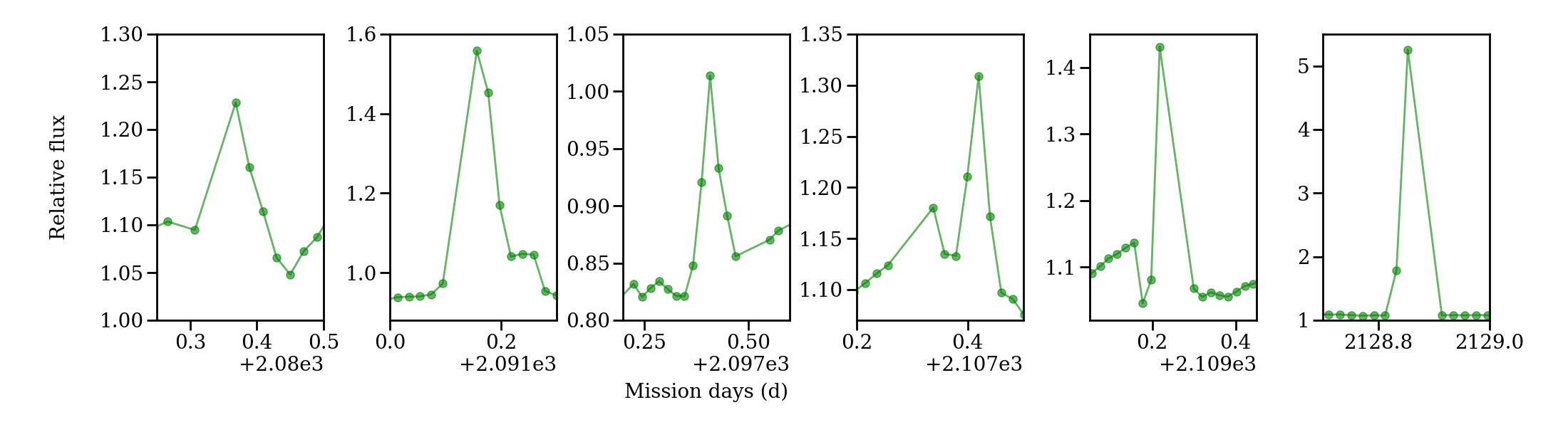
Figure 16: Observed flares.

Despite the mild accretion, there are signatures of activity. There are several brief increases in brightness in the K2 data that could be stellar flares (see Table 6). All the cases were checked against contamination from Solar System objects, which can mimic the flaring behavior (Rappaport et al., 2019), using SkyBot (Berthier et al., 2006, 2016) as done by (Szabó et al., 2015), and no contamination was detected (Martti Holst Kristiansen, private communication). In 5 cases, the increased flux is detected in at least 3 datapoints, revealing a profile consistent with stellar flares (Doyle et al., 2018; Gershberg & Shakhovskaia, 1983), with a sharp rise and slower decline and duration between 1-3h (see Figure 16). Four more potential events are detected in less than 3 observations (consistent with short flares, Doyle et al., 2018, but also harder to confirm) and/or are weaker. One among them happens during an eclipse, so their classification is more uncertain. One of them (on MJD 59021.611483) has extreme intensity, although it does not show the usual flare profile (rapid rise, slower decay), but rises over two observations and falls of from the peak within half an hour. The two largest flares happen at the beginning and at the end of the period between 2091-2010d when the star also presents concatenated eclipses, but more data would be needed to tell whether this is significant. One of the flaring events may be composed of at least two consecutive flares, as it has been observed in some M-type stars (Doyle et al., 2018). No flares are detected in the REM data, likely due to the sparse sampling.

Table 6: Flares detected in the K2 data.

MJD	Strength	Duration	Notes
(d)	(vs cont.)	(h)
58973.147562	1.2	1.5	Weak
58983.935503	1.5	1.5	Possible tail up to 1.5h more
58985.406582	1.5	1.5	During eclipse, uncertain
58990.146722	1.2	2.5	Rise and fall observed
59000.117352	1.2	2.5	Messy, could be 2 flares
59001.997061	1.3	0.5:	Single datapoint, uncertain
59015.502389	1.4	0.5:	Single datapoint, uncertain
59021.611483	4.9	2.0	Very strong, 2 points
59023.082572	1.1	1.5	Weak, 2 points

Appendix C Summary of the kinematics from optical spectroscopy

Table 7 lists the rotational and radial velocities derived for all the individual Keck spectra. The rotational and radial velocities are consistent throughout all the spectra, although the quality of the data from MJD 55287.614 is better than the others. There is no evidence of radial velocity variability within the observed errors. Constraining the possible radial velocity companions with sparse-sampled data in an object with variable accretion and quasi-stable accretion columns along the line-of-sight would require a detailed analysis to distinguish accretion and gas absorption from the disk from those of potential companions (e.g. see Mora et al., 2002; Sicilia-Aguilar et al., 2015) that is beyond the scope of this paper. Note that the spectra from 54689.304 and 55256.556 are noisier than the rest in the regions used for the velocity estimates, and thus the results are highly uncertain.

Table 7: HIRES/Keck radial and rotational velocities.

MJD	Rad. Vel.	v$sini$
(d)	(km/s)	(km/s)
53902.275	-6.6$\pm$0.6	16.7$\pm$0.4
53902.278	-6.8$\pm$0.4	16.6$\pm$0.7
54642.417	-4.4$\pm$0.7	17.7$\pm$0.5
54689.304	-5.7$\pm$1.5∗	18$\pm$2∗
55256.556	-7.7$\pm$0.3∗	11$\pm$2∗
55287.614	-6.8$\pm$0.1	16.2$\pm$0.6

Appendix D Archival SED photometry

Table 8 contains the archival photometry from VizieR that we selected as being most likely representative for the out-of-eclipse SED. We chose the brightest magnitudes observed in each filter, adding also those that are unlikely to change due to extinction and on short timescales (mid-IR and longer wavelengths). Due to the non-homogeneity of the sample and to the lack of detailed knowledge of the full spectrum variability, some of the selected points may have been taken during eclipse phases.

Table 8: Archival SED data during the out-of-eclipse phases.

$\lambda$	Fν	Survey	Reference
(Å)	(Jy)
0.350	0.0014$\pm$0.0001	SkyMapper u	W18
0.387	0.0045$\pm$0.0004	SkyMapper v	W18
0.420	0.0286	HIPPARCOS BT	U01
0.444	0.0171$\pm$0.0086	Johnson B	H15
0.444	0.0188$\pm$0.0076	Johnson B	H15
0.468	0.0215$\pm$0.0068	POSS-II J	L08
0.482	0.026$\pm$0.012	SDSS g′	H15
0.497	0.0403$\pm$0.0027	SkyMapper g	W18
0.505	0.0329$\pm$0.0015	GAIA DR2 Gbp	D19
0.554	0.045$\pm$0.019	Johnson V	H15
0.604	0.067$\pm$0.005	SkyMapper r	W18
0.623	0.059$\pm$0.001	GAIA DR2 G	D19
0.625	0.071$\pm$0.028	SDSS r′	H15
0.763	0.105$\pm$0.044	SDSS i′	H15
0.772	0.110$\pm$0.004	GAIA DR2 Grp	D19
0.784	0.123$\pm$0.039	POSS-II i	L08
0.865	0.164	PAN-STARRS z	C16
3.35	0.293$\pm$0.006	WISE W1	C12
4.6	0.251$\pm$0.004	WISE W2	C12
11.6	0.0614$\pm$0.0008	WISE W3	C12
22.1	0.152$\pm$0.003	WISE W4	C12
23.7	0.173$\pm$0.006	Spitzer/MIPS 24	E18
65	2.7	AKARI N60	Y10
90	3.15$\pm$0.25	AKARI WIDE-S	Y10
134	5.3$\pm$1.0	AKARI WIDE-L	Y10
160	2.62	AKARI N160	Y10
880	0.219$\pm$0.001	ALMA	B16

References

- Alencar et al. (2012) Alencar, S. H. P., Bouvier, J., Walter, F. M., et al. 2012, A&A, 541, A116
- Alencar et al. (2018) Alencar, S. H. P., Bouvier, J., Donati, J.-F., et al. 2018, A&A, 620, A195
- Ansdell et al. (2016) Ansdell, M., Gaidos, E., Williams, J. P., et al. 2016, MNRAS, 462, L101.
- Astropy Collaboration et al. (2013) Astropy Collaboration, Robitaille, T. P., Tollerud, E. J., et al. 2013, A&A, 558, A33
- Astropy Collaboration et al. (2018) Astropy Collaboration, Price-Whelan, A. M., Sipőcz, B. M., et al. 2018, AJ, 156, 123
- Baraffe et al. (2015) Baraffe, I., Homeier, D., Allard, F., et al. 2015, A&A, 577, A42
- Barenfeld et al. (2016) Barenfeld, S. A., Carpenter, J. M., Ricci, L., et al. 2016, ApJ, 827, 142
- Benisty et al. (2017) Benisty, M., Stolker, T., Pohl, A., et al. 2017, A&A, 597, A42
- Benisty et al. (2018) Benisty, M., Juhász, A., Facchini, S., et al. 2018, A&A, 619, A171
- Berthier et al. (2006) Berthier, J., Vachier, F., Thuillot, W., et al. 2006, Astronomical Data Analysis Software and Systems XV, 367
- Berthier et al. (2016) Berthier, J., Carry, B., Vachier, F., et al. 2016, MNRAS, 458, 3394
- Bessell & Brett (1988) Bessell, M.S. & Brett, J.M., 1988, PASP, 100, 113
- Bessell (2005) Bessell, M. S. 2005, ARA&A, 43, 293.
- Bodman et al. (2017) Bodman, E. H. L., Quillen, A. C., Ansdell, M., et al. 2017, MNRAS, 470, 202
- Bouvier et al. (1999) Bouvier, J., Chelli, A., Allain, S., et al. 1999, A&A, 349, 619.
- Bouvier et al. (2007) Bouvier, J., Alencar, S. H. P., Boutelier, T., et al. 2007, A&A, 463, 1017
- Bozhinova et al. (2016) Bozhinova, I., Scholz, A., & Eislöffel, J. 2016, MNRAS, 458, 3118
- Bozhinova et al. (2016) Bozhinova, I., Scholz, A., Costigan, G., et al. 2016, MNRAS, 463, 4459
- Brumberg (1991) Brumberg, V. A. 1991, Bristol
- Canovas et al. (2017) Canovas, H., Hardy, A., Zurlo, A., et al. 2017, A&A, 598, A43.
- Cardelli et al. (1989) Cardelli, J. A., Clayton, G. C., & Mathis, J. S. 1989, Interstellar Dust, 5.
- Carpenter et al. (2006) Carpenter, J. M., Mamajek, E. E., Hillenbrand, L. A., et al. 2006, ApJ, 651, L49
- Carpenter et al. (2009) Carpenter, J. M., Mamajek, E. E., Hillenbrand, L. A., et al. 2009, ApJ, 705, 1646
- Carpenter et al. (2014) Carpenter, J. M., Ricci, L., & Isella, A. 2014, ApJ, 787, 42
- Chambers et al. (2016) Chambers, K. C., Magnier, E. A., Metcalfe, N., et al. 2016, arXiv e-prints, arXiv:1612.05560
- Cohen et al. (2003) Cohen, M., Wheaton, W. A., & Megeath, S. T. 2003, AJ, 126, 1090
- Curcio et al. (1964) Curcio, J., Drummeler, L., Knestrick,G., 1964, Applied Optics Vol. 3, N. 12, 1401
- Cutri, & et al. (2012) Cutri, R. M., & et al. 2012, VizieR Online Data Catalog, II/311
- Dahm, & Carpenter (2009) Dahm, S. E., & Carpenter, J. M. 2009, AJ, 137, 4024
- Dahm et al. (2012) Dahm, S. E., Slesnick, C. L., & White, R. J. 2012, ApJ, 745, 56.
- D’Alessio et al. (2006) D’Alessio, P., Calvet, N., Hartmann, L., et al. 2006, ApJ, 638, 314
- Damiani et al. (2019) Damiani, F., Prisinzano, L., Pillitteri, I., et al. 2019, A&A, 623, A112
- Davies (2019) Davies, C. L. 2019, MNRAS, 484, 1926.
- Donati et al. (2019) Donati, J.-F., Bouvier, J., Alencar, S. H., et al. 2019, MNRAS, 483, L1
- Doyle et al. (2018) Doyle, L., Ramsay, G., Doyle, J. G., et al. 2018, MNRAS, 480, 2153.
- Drake et al. (2009) Drake, A. J., Djorgovski, S. G., Mahabal, A., et al. 2009, ApJ, 696, 870
- Dullemond et al. (2003) Dullemond, C. P., van den Ancker, M. E., Acke, B., et al. 2003, ApJ, 594, L47
- Dong et al. (2017) Dong, R., van der Marel, N., Hashimoto, J., et al. 2017, ApJ, 836, 201
- Dullemond & Dominik (2004) Dullemond, C., & Dominik, C., 2004, A&A, 417, 159
- Dullemond (2011) Dullemond, C. P. 2011, RADMC: A 2-D Continuum Radiative Transfer Tool, ascl:1108.016
- Dupree et al. (2012) Dupree, A. K., Brickhouse, N. S., Cranmer, S. R., et al. 2012, ApJ, 750, 73
- Duschl et al. (1996) Duschl, W. J., Gail, H.-P., & Tscharnuter, W. M. 1996, A&A, 312, 624
- Eiroa et al. (2002) Eiroa, C., Oudmaijer, R., et al., 2002, A&A 384, 1038
- Espaillat et al. (2011) Espaillat, C., Furlan, E., D’Alessio, P., et al. 2011, ApJ, 728, 49
- Esplin et al. (2018) Esplin, T. L., Luhman, K. L., Miller, E. B., et al. 2018, AJ, 156, 75
- Fang et al. (2014) Fang, M., Sicilia-Aguilar, A., Roccatagliata, V., et al. 2014, A&A, 570, A118
- Flaherty et al. (2012) Flaherty, K. M., Muzerolle, J., Rieke, G., et al. 2012, ApJ, 748, 71
- Flewelling et al. (2016) Flewelling, H. A., Magnier, E. A., Chambers, K. C., et al. 2016, arXiv e-prints, arXiv:1612.05243
- Fonseca et al. (2014) Fonseca, N. N. J., Alencar, S. H. P., Bouvier, J., et al. 2014, A&A, 567, A39
- Ford et al. (2000) Ford, E. B., Kozinsky, B., & Rasio, F. A. 2000, ApJ, 535, 385
- Frescura et al. (2008) Frescura, F. A. M., Engelbrecht, C. A., & Frank, B. S. 2008, MNRAS, 388, 1693.
- Fukugita et al. (1996) Fukugita, M., Ichikawa, T., Gunn, J. E., et al. 1996, AJ, 111, 1748
- Gaia Collaboration et al. (2016) Gaia Collaboration, Prusti, T., de Bruijne, J. H. J., et al. 2016, A&A, 595, A1
- Gaia Collaboration et al. (2018) Gaia Collaboration, Brown, A. G. A., Vallenari, A., et al. 2018, arXiv:1804.09365
- Gaia Collaboration (2018) Gaia Collaboration 2018, VizieR Online Data Catalog, 1345
- Gershberg & Shakhovskaia (1983) Gershberg, R. E., & Shakhovskaia, N. I. 1983, Ap&SS, 95, 235.
- Grankin et al. (2007) Grankin, K. N., Melnikov, S. Y., Bouvier, J., et al. 2007, A&A, 461, 183
- Grinin (1988) Grinin, V. P. 1988, Soviet Astronomy Letters, 14, 27
- Grinin et al. (2008) Grinin, V., Stempels, H. C., Gahm, G. F., et al. 2008, A&A, 489, 1233
- Grinsted et al. (2004) Grinsted, A., Moore, J. C., & Jevrejeva, S. 2004, Nonlinear Processes in Geophysics, 11, 561.
- Gustafsson et al. (2008) Gustafsson, B., et al. 2008, A&A 486, 951
- Hamann & Persson (1992) Hamann, F., & Persson, S. E. 1992, ApJS, 82, 247
- Heinze et al. (2018) Heinze, A. N., Tonry, J. L., Denneau, L., et al. 2018, AJ, 156, 241
- Henden et al. (2015) Henden, A. A., Levine, S., Terrell, D., et al. 2015, American Astronomical Society Meeting Abstracts #225 225, 336.16
- Horne & Baliunas (1986) Horne, J. H., & Baliunas, S. L. 1986, ApJ, 302, 757
- Huber et al. (2016) Huber, D., Bryson, S. T., Haas, M. R., et al. 2016, ApJS, 224, 2.
- Isella & Natta (2005) Isella, A., & Natta, A. 2005, A&A, 438, 899
- Jäger et al. (2003) Jäger, C., Fabian, D., et al. 2003, A&A, 401, 57
- Kama et al. (2009) Kama, M., Min, M., & Dominik, C. 2009, A&A, 506, 1199
- Kenyon & Hartmann (1995) Kenyon, S.J. & Hartmann, L., 1995, ApJS , 101, 117
- Köhler et al. (2000) Köhler, R., Kunkel, M., Leinert, C., et al. 2000, A&A, 356, 541.
- Kozai (1962) Kozai, Y. 1962, AJ, 67, 591
- Kraus et al. (2008) Kraus, A. L., Ireland, M. J., Martinache, F., et al. 2008, ApJ, 679, 762.
- Kurosawa, & Romanova (2013) Kurosawa, R., & Romanova, M. M. 2013, MNRAS, 431, 2673
- Laibe et al. (2014) Laibe, G., Gonzalez, J.-F., Maddison, S. T., et al. 2014, MNRAS, 437, 3055
- Lasker et al. (2008) Lasker, B. M., Lattanzi, M. G., McLean, B. J., et al. 2008, AJ, 136, 735
- Liu et al. (2007) Liu, Y., San Liang, X., & Weisberg, R. H. 2007, Journal of Atmospheric and Oceanic Technology, 24, 2093.f
- Loomis et al. (2017) Loomis, R. A., Öberg, K. I., Andrews, S. M., et al. 2017, ApJ, 840, 23
- Luhman et al. (2003) Luhman, K. L., Stauffer, J. R., Muench, A. A., et al. 2003, ApJ, 593, 1093
- Luhman & Mamajek (2012) Luhman, K. L., & Mamajek, E. E. 2012, ApJ, 758, 31
- Magnier et al. (2016) Magnier, E. A., Schlafly, E. F., Finkbeiner, D. P., et al. 2016, arXiv e-prints, arXiv:1612.05242
- Marino et al. (2015) Marino, S., Perez, S., & Casassus, S. 2015, ApJ, 798, L44
- Mathews et al. (2012) Mathews, G. S., Williams, J. P., Ménard, F., et al. 2012, ApJ, 745, 23
- Mathews et al. (2013) Mathews, G. S., Pinte, C., Duchêne, G., et al. 2013, A&A, 558, A66
- Mayama et al. (2018) Mayama, S., Akiyama, E., Panić, O., et al. 2018, ApJ, 868, L3
- McClure et al. (2013) McClure, M. K., D’Alessio, P., Calvet, N., et al. 2013, ApJ, 775, 114
- McGinnis et al. (2015) McGinnis, P. T., Alencar, S. H. P., Guimarães, M. M., et al. 2015, A&A, 577, A11
- Mihalas (1978) Mihalas, D. 1978, San Francisco: W.H. Freeman
- Miyake & Nakagawa (1993) Miyake, K., & Nakagawa, Y., 1993, ICARUS, 106, 20
- Mora et al. (2002) Mora, A., Natta, A., Eiroa, C., et al. 2002, A&A, 393, 259
- Mortier & Collier Cameron (2017) Mortier, A., & Collier Cameron, A. 2017, A&A, 601, A110.
- Natta et al. (2004) Natta, A., Testi, L., Muzerolle, J., et al. 2004, A&A, 424, 603
- Ochsenbein et al. (2000) Ochsenbein, F., Bauer, P., & Marcout, J. 2000, A&AS, 143, 23
- Panić et al. (2009) Panić, O., Hogerheijde, M. R., Wilner, D., & Qi, C. 2009, A&A, 501, 269
- Pecaut et al. (2012) Pecaut, M. J., Mamajek, E. E., & Bubar, E. J. 2012, ApJ, 746, 154
- Pecaut, & Mamajek (2016) Pecaut, M. J., & Mamajek, E. E. 2016, MNRAS, 461, 794
- Pinilla et al. (2015) Pinilla, P., de Boer, J., Benisty, M., et al. 2015, A&A, 584, L4
- Pinilla et al. (2018) Pinilla, P., Benisty, M., de Boer, J., et al. 2018, ApJ, 868, 85.
- Predehl & Schmitt (1995) Predehl, P., & Schmitt, J. H. M. M. 1995, A&A, 293, 889
- Preibisch & Zinnecker (1999) Preibisch, T., & Zinnecker, H. 1999, AJ, 117, 2381.
- Rappaport et al. (2019) Rappaport, S., Zhou, G., Vanderburg, A., et al. 2019, MNRAS, 485, 2681
- Rebull et al. (2018) Rebull, L. M., Stauffer, J. R., Cody, A. M., et al. 2018, AJ, 155, 196.
- Riviere-Marichalar et al. (2013) Riviere-Marichalar, P., Pinte, C., Barrado, D., et al. 2013, A&A, 555, A67
- Roccatagliata et al. (2013) Roccatagliata, V. and Preibisch, T. and Ratzka, T. and Gaczkowski, B., 2013, A&AA6, 554
- Rodrigues et al. (2014) Rodrigues, T. S., Girardi, L., Miglio, A., et al. 2014, MNRAS, 445, 2758
- Scargle (1982) Scargle, J. D. 1982, ApJ, 263, 835.
- Schneider et al. (2018) Schneider, P. C., Manara, C. F., Facchini, S., et al. 2018, A&A, 614, A108
- Scholz et al. (2019) Scholz, A., Natta, A., Bozhinova, I., et al. 2019, MNRAS, 484, 4260.
- Schlegel et al. (1998) Schlegel, D. J., Finkbeiner, D. P., & Davis, M. 1998, ApJ, 500, 525
- Sicilia-Aguilar et al. (2005) Sicilia-Aguilar, A., Hartmann, L., Szentgyorgyi, A., Roll, J., Conroy, M., Calvet, N., Fabricant, D., & Hernández, J., 2005a, AJ, 129, 363
- Sicilia-Aguilar et al. (2008) Sicilia-Aguilar, A., Merín, B., Hormuth, F., et al. 2008, ApJ, 673, 382.
- Sicilia-Aguilar et al. (2012) Sicilia-Aguilar, A., Kóspál, Á., Setiawan, J., et al. 2012, A&A, 544, A93
- Sicilia-Aguilar et al. (2015) Sicilia-Aguilar, A., Fang, M., Roccatagliata, V., et al. 2015, A&A, 580, A82
- Sicilia-Aguilar et al. (2017) Sicilia-Aguilar, A., Oprandi, A., Froebrich, D., et al. 2017, A&A, 607, A127.
- Siess et al. (2000) Siess, L., Dufour, E. & Forestini, M. 2000 A&A , 358, 593
- Siwak et al. (2014) Siwak, M., Rucinski, S. M., Matthews, J. M., et al. 2014, MNRAS, 444, 327
- Skrutskie et al. (2006) Skrutskie, M. F., Cutri, R. M., Stiening, R., et al. 2006, AJ, 131, 1163.
- Stoughton et al. (2002) Stoughton, C., Lupton, R. H., Bernardi, M., et al. 2002, AJ, 123, 485
- Szabó et al. (2015) Szabó, R., Sárneczky, K., Szabó, G. M., et al. 2015, AJ, 149, 112
- Tielens et al. (2005) Tielens, A. G. G. M., Waters, L. B. F. M., & Bernatowicz, T. J. 2005, Chondrites and the Protoplanetary Disk, 605
- Torrence, & Compo (1998) Torrence, C., & Compo, G. P. 1998, Bulletin of the American Meteorological Society, 79, 61.
- Urban et al. (2001) Urban, S. E., Corbin, T. E., Wycoff, G. L., et al. 2001, American Astronomical Society Meeting Abstracts 199, 129.04
- Vogt et al. (1994) Vogt, S. S., Allen, S. L., Bigelow, B. C., et al. 1994, Instrumentation in Astronomy VIII, 362.
- Weise et al. (2010) Weise, P., Launhardt, R., Setiawan, J., et al. 2010, A&A, 517, A88
- Wenger et al. (2000) Wenger, M., Ochsenbein, F., Egret, D., et al. 2000, A&AS, 143, 9
- Zechmeister, & Kürster (2009) Zechmeister, M., & Kürster, M. 2009, A&A, 496, 577.
- Wolf et al. (2018) Wolf, C., Onken, C. A., Luvaul, L. C., et al. 2018, PASA, 35, e010
- Wright et al. (2010) Wright, E. L., Eisenhardt, P. R. M., Mainzer, A. K., et al. 2010, AJ, 140, 1868
- Yamamura et al. (2010) Yamamura, I., Makiuti, S., Ikeda, N., et al. 2010, VizieR Online Data Catalog, II/298
- Zacharias et al. (2004) Zacharias, N., Urban, S. E., Zacharias, M. I., et al. 2004, AJ, 127, 3043
- Zhang et al. (2014) Zhang, K., Isella, A., Carpenter, J. M., et al. 2014, ApJ, 791, 42.