Localization landscape for Dirac fermions

Abstract

In the theory of Anderson localization, a landscape function predicts where wave functions localize in a disordered medium, without requiring the solution of an eigenvalue problem. It is known how to construct the localization landscape for the scalar wave equation in a random potential, or equivalently for the Schrödinger equation of spinless electrons. Here we generalize the concept to the Dirac equation, which includes the effects of spin-orbit coupling and allows to study quantum localization in graphene or in topological insulators and superconductors. The landscape function $u(\bm{r})$ is defined on a lattice as a solution of the differential equation $\overbracket{{H}}u(\bm{r})=1$, where $\overbracket{{H}}$ is the Ostrowsky comparison matrix of the Dirac Hamiltonian. Random Hamiltonians with the same (positive definite) comparison matrix have localized states at the same positions, defining an equivalence class for Anderson localization. This provides for a mapping between the Hermitian and non-Hermitian Anderson model.

Introduction — The localization landscape is a new tool in the study of Anderson localization, pioneered in 2012 by Filoche and Mayboroda Fil12 , which has since stimulated much computational and conceptual progress Fil13 ; Arn16 ; Ste17 ; Fil17 ; Pic17 ; Li17 ; Cha19 ; Arn19 ; Har18 ; Bee19 . The “landscape” of a Hamiltonian $H$ is a function $u(\bm{r})$ that provides an upper bound for eigenstates $\psi$ at energy $E>0$:

$$|\psi(\bm{r})|/|\psi|_{\rm max}\leq E\,u(\bm{r}),\;\;|\psi|_{\rm max}=\textstyle{\max_{\bm{r}}}|\psi(\bm{r})|.$$ (1)

This inequality implies that a localized state is confined to spatial regions where $u\gtrsim 1/E$. Extensive numerical simulations Arn19 confirm the expectation that higher and higher peaks in $u$ identify the location of states at smaller and smaller $E$.

Such a predictive power would be unremarkable for particles confined to potential wells (deeper and deeper wells trap particles at lower and lower energies). But Anderson localization happens because of wave interference in a random “white noise” potential, and inspection of the potential landscape $V(\bm{r})$ gives no information on the localization landscape $u(\bm{r})$.

Filoche and Mayboroda considered the localization of scalar waves, or equivalently of spinless electrons, governed by the Schrödinger Hamiltonian $H=-\nabla^{2}+V$. They used the maximum principle for elliptic partial differential equations to derive Fil12 that the inequality (1) holds if $V>0$ and $u$ is the solution of

$$[-\nabla^{2}+V(\bm{r})]u(\bm{r})=1.$$ (2)

Our objective here is to generalize this to spinful electrons, to include the effects of spin-orbit coupling and study localization of Dirac fermions.

Construction of the landscape function — Our key innovation is to use Ostrowski’s comparison matrix Ost37 ; Ost56 ; nomenclature ; Ber94 as a general framework for the construction of a localization landscape on a lattice. By definition, the comparison matrix $\overbracket{{H}}$ of a complex matrix ${{H}}$ has elements

$${\overbracket{{H}}}_{nm}=\begin{cases}|{{H}}_{nn}|&{\rm if}\;\;n=m,\\ -|{{H}}_{nm}|&{\rm if}\;\;n\neq m.\end{cases}$$ (3)

In our context the index $n=1,2,\ldots$ labels both the discrete space coordinates as well as any internal (spinor) degrees of freedom. The comparison theorem Ost37 states that if the comparison matrix is positive-definite, then note1

$$|{{H}}^{-1}|\leq{\overbracket{{H}}}\,^{-1},$$ (4)

where both the absolute value and the inequality is taken elementwise.

We apply Eq. (4) to an eigenstate $\Psi$ of ${{H}}$ at energy $E$,

$$|E^{-1}\Psi_{n}| =|({{H}}^{-1}\Psi)_{n}|\leq\textstyle{\sum_{m}}\bigl{|}\bigl{(}{{H}}\,^{-1}\bigr{)}_{nm}\bigr{|}|\Psi_{m}|$$

$$\leq|\Psi|_{\rm max}\textstyle{\sum_{m}}\bigl{(}{\overbracket{{H}}}\,^{-1}\bigr{)}_{nm},$$ (5)

with $|\Psi|_{\rm max}=\max_{n}|\Psi_{n}|$. We now define a landscape function $u$ with elements $u_{n}$ in terms of a set of linear equations with coefficients given by the comparison matrix:

$$\overbracket{H}u=1\Leftrightarrow\textstyle{\sum_{m}}{\overbracket{{H}}}_{nm}u_{m}=1,\;\;n=1,2,\ldots N,$$ (6)

which implies that

$$\textstyle{\sum_{m}}\bigl{(}{\overbracket{{H}}}\,^{-1}\bigr{)}_{nm}=u_{n}.$$ (7)

Substitution into Eq. (5) thus gives the desired inequality

$$|\Psi_{n}|/|\Psi|_{\rm max}\leq|E|\,u_{n}.$$ (8)

As a sanity check, we make contact with the original landscape function Fil12 for the Schrödinger Hamiltonian $H_{\rm S}=p^{2}/2m+V$, with $V>0$. The Laplacian is discretized in terms of nearest-neighbor hoppings on a lattice. For each dimension

$$\begin{split}&p^{2}\mapsto(\hbar/a)^{2}(2-2\cos ka)\Rightarrow\\ &(H_{\rm S})_{nm}=t_{0}(2\delta_{nm}-\delta_{n-1,m}-\delta_{n+1,m})+V_{n}\delta_{nm},\end{split}$$ (9)

with lattice constant $a$ and hopping matrix element $t_{0}=\hbar^{2}/2ma^{2}$. The comparison matrix ${\overbracket{H}}_{\rm S}$ is equal to $H_{\rm S}$ and is positive-definite, so that Eq. (6) is a discretized version of the original landscape equation $H_{\rm S}u=1$ Fil12 ; Lyr15 .

Rashba Hamiltonian — Our first novel application is to introduce spin-orbit coupling of the Rashba form,

$$H_{\rm R}=H_{\rm S}+\tfrac{1}{2}\{\lambda,p_{x}\}\sigma_{y}-\tfrac{1}{2}\{\lambda,p_{y}\}\sigma_{x}.$$ (10)

(The anticommutator $\{\cdots\}$ enforces Hermiticity when $\lambda$ is spatially dependent.) The comparison matrix is now no longer equal to the Hamiltonian, in 1D one has

$$({\overbracket{H}}_{\rm R})_{ij}=(H_{\rm S})_{ij}-\frac{\hbar}{4a}|\lambda_{i}+\lambda_{j}|(\delta_{i-1,j}+\delta_{i+1,j})\sigma_{x}.$$ (11)

The $i,j,$ indices label the spatial positions, the spinor indices are implicit in the Pauli matrix.

As a test, to isolate the effect of spin-orbit coupling, we place all the disorder in the Rashba strength $\lambda_{n}$, which fluctuates randomly from site to site, uniformly in the interval $(\bar{\lambda}-\delta\lambda,\bar{\lambda}+\delta\lambda)$. The electrostatic potential is a constant offset $V_{0}$, chosen sufficiently large that ${\overbracket{H}}_{\rm R}$ is positive-definite note2 . Examples in 1D and in 2D are shown in Figs. 1 and 2. The highest peaks in the landscape function match well with the lowest eigenfunctions.

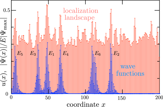
Figure 1: Landscape function $u(x)$ (red) and normalized wave function profile $|\Psi(x)|/E|\Psi_{\rm max}|$ (blue) for the 6 lowest (twofold degenerate) eigenstates of the disordered 1D Rashba Hamiltonian (11) (parameters $V_{0}=4t_{0}$, $\bar{\lambda}=0$, $\delta\lambda=3\hbar/a$, hard-wall boundary conditions). The 1D array has $n=1,2,\ldots 200$ sites, in the plot $x=n$ shows the first spinor component and $x=n+1/2$ shows the second spinor component. The wave functions are labeled by the corresponding energy levels $\{E_{1},\ldots E_{6}\}=\{3.273,3.3371,3.414,3.446,3.508,3.516\}$ (in units of $t_{0}$).

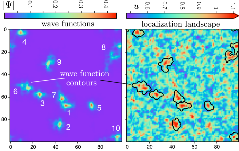
Figure 2: Same comparison as in Fig. 1, but now for the 2D Rashba Hamiltonian, discretized on a $100\times 100$ square lattice (parameters $V_{0}=6t_{0}$, $\bar{\lambda}=2\delta\lambda=2\hbar/a$, periodic boundary conditions).The left panel shows the spinor norm $|\Psi_{n}(\bm{r)}|$ for the 10 lowest (twofold degenerate) eigenstates of ${{H}}_{\rm R}$. The right panel shows the localization landscape. The black contours (computed at 10% of the peak height of $|\Psi|$) identify the location of the 10 eigenstates — to show the close correspondence with the local maxima of $u(\bm{r})$.

Dirac Hamiltonian — We next turn to Dirac fermions, first in 1D. The Dirac Hamiltonian

$$H_{\rm D}=v_{\rm F}p_{x}\sigma_{x}+V\sigma_{0}+\mu\sigma_{z}$$ (12)

contains a scalar potential $V$ proportional to the $2\times 2$ unit matrix $\sigma_{0}$ and a staggered potential $\mu$ proportional to $\sigma_{z}$, acting on the two-component wave function $\Psi=(\psi_{A},\psi_{B})$. This would apply to a graphene nanoribbon on a substrate such as hexagonal boron nitride, which differentiates between the two carbon atoms in the unit cell without causing intervalley scattering Gio07 .

The symmetric discretization $\partial_{x}\Psi\mapsto(1/2a)[\Psi(x+a)-\Psi(x-a)]$ suffers from fermion doubling Sta82 ; Two08 — it corresponds to a $\sin ka$ dispersion with a second species of massless Dirac fermions at the edge of the Brillouin zone ($k=\pi/a$). To avoid this, and restrict ourselves to a single valley, we use a staggered-fermion discretization a la Susskind Sus77 ; Her12 :

$$p_{x}\sigma_{x}\Psi\mapsto(-i\hbar/a)\begin{pmatrix}\psi_{B}(x)-\psi_{B}(x-a)\\ \psi_{A}(x+a)-\psi_{A}(x)\end{pmatrix}.$$ (13)

The corresponding dispersion note4

$$E(k)=\pm t_{1}\sqrt{2-2\cos ka},\;\;t_{1}=\hbar v_{\rm F}/a,$$ (14)

has massless fermions only at the center of the Brillouin zone ($k=0$).

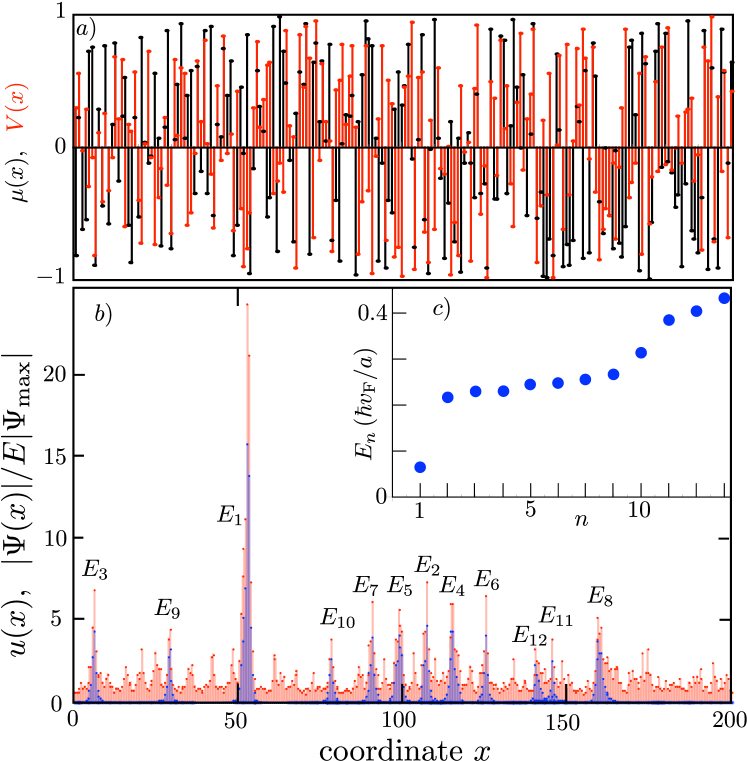
Figure 3: Panel (a): Random scalar potential $V(x)$ (red) and staggered potential $\mu(x)$ (black) for the 1D Dirac Hamiltonian (12) (parameters $\bar{V}=3t_{1}$, $\bar{\mu}=0$, $\delta V=\delta\mu=t_{1}$, hard-wall boundary conditions). Panel b): Corresponding localization landscape (red) and eigenfunctions of the 12 lowest energy levels (blue), at energies $E_{n}$ near the band edge plotted in the inset (panel c). The peaks in the localization landscape are not correlated in any obvious way with the random potentials, but they accurately predict the location of the low-lying modes.

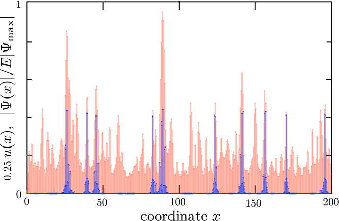
Figure 4: Same as Fig. 3b, but now for a gapped system ($\bar{V}=\delta V=0$, $\bar{\mu}=3.5\,t_{1}$, $\delta\mu=1.5\,t_{1}$). The eigenfunctions of the 20 levels closest to the gap are shown (blue, $2.3\,t_{1}<|E_{n}|<2.5\,t_{1}$). There are only 10 distinct peaks, because of an approximate $\pm E$ symmetry. The landscape function (red, rescaled by a factor $1/4$) accurately identifies the location of the states near the gap.

The comparison matrix takes the form

$$({\overbracket{{H}}}_{\rm D})_{ij}=\begin{pmatrix}|V_{i}+\mu_{i}|\delta_{ij}&-t_{1}(\delta_{ij}+\delta_{i+1,j})\\ -t_{1}(\delta_{ij}+\delta_{i-1,j})&|V_{i}-\mu_{i}|\delta_{ij}\end{pmatrix}.$$ (15)

We take random $V(x)\in(\bar{V}-\delta V,\bar{V}+\delta V)$ and $\mu(x)\in(\bar{\mu}-\delta\mu,\bar{\mu}+\delta\mu)$, chosen independently and uniformly at each lattice site. The condition $|V_{i}\pm\mu_{i}|>2t_{1}$ ensures a positive-definite ${\overbracket{{H}}}_{\rm D}$. As shown in Figs. 3 and 4, the landscape function computed from ${\overbracket{{H}}}_{\rm D}u=1$ again accurately identifies the locations of the low-lying eigenfunctions (near the band edge in Fig. 3 and near the gap in Fig. 4).

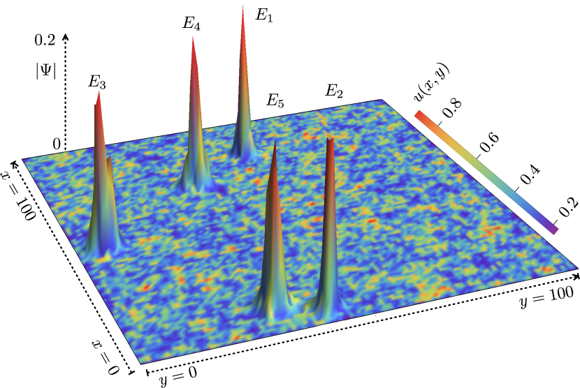
Figure 5: Comparison of the landscape function (2D color scale plot) with wave function amplitudes (3D profile) of the chiral p-wave superconductor with Hamiltonian (16) (parameters $\Delta=1$, $\bar{V}=6$, $\delta V=4$, in units of $t_{0}=\hbar^{2}/2ma^{2}$). The wave functions show the five Andreev levels with smallest $E_{n}>0$ ($E_{1},E_{2},\ldots E_{5}=3.763,3.799,3.875,3.882,3.893$). (The charge-conjugate states at $-E_{n}$ have the same spinor amplitude $|\Psi|$.) The colors of the wave function profile correspond to the landscape function, so a red wave function peak indicates that $u(x,y)$ peaks at the same position.

For the 2D Dirac equation we consider a chiral p-wave superconductor, with Bogoliubov-De Gennes Hamiltonian Bee16

$${{H}}_{\rm BdG}=\Delta(p_{x}\sigma_{x}+p_{y}\sigma_{y})+(V+p^{2}/2m)\sigma_{z}.$$ (16)

The Pauli matrices act on the electron-hole degree of freedom of a Bogoliubov quasiparticle, and the Hamiltonian is constrained by particle-hole symmetry: $\sigma_{x}H_{\rm BdG}\sigma_{x}=-H_{\rm BdG}^{\ast}$. (A scalar offset $\propto\sigma_{0}$ is thus forbidden.) The pair potential $\Delta$ opens a gap in the spectrum in the entire Brillouin zone, provided that the electrostatic potential $V$ is nonzero. The gap-closing transition at $V=0$ is a topological phase transition Rea00 .

We take a uniform real $\Delta$ (no vortices) and a disordered $V(x,y)$, fluctuating randomly from site to site in the interval $(\bar{V}+\delta V,\bar{V}-\delta V)$. Positive $V$ ensures we do not cross the gap-closing transition, so we will not be introducing Majorana zero-modes Wim10 (the levels are Andreev bound states). Unlike in the case of graphene we can use the symmetric discretization $p\mapsto\sin ka$ — there is no need for a staggered discretization because the kinetic energy $p^{2}\mapsto 2-2\cos ka$ prevents fermion doubling at $k=\pi/a$. Results are shown in Fig. 5.

Equivalence classes — In the final part of this paper we move beyond applications to address a conceptual implication of the theory. Two complex matrices $A,B$ are called equimodular if $|A_{nm}|=|B_{nm}|$. By the construction (3), they have the same comparison matrix, $\overbracket{A}=\overbracket{B}$, and therefore the same landscape function $u_{A}=u_{B}$, uniquely determined by the same equation $\overbracket{A}u_{A}=1=\overbracket{B}u_{B}$. We thus obtain an equivalence class for Anderson localization: Equimodular Hamiltonians have localized states at the same position, identified by peaks in the landscape function.

We have checked this for the 2D Rashba Hamiltonian (10): Randomly varying the sign of the coefficient $\lambda(\bm{r})$ from site to site shifts the energy levels around, but the states remain localized at the same positions. More generally, one could try to vary the coefficients over the complex plane, preserving the norm. This would produce a non-Hermitian eigenvalue problem, and one might wonder whether the whole approach breaks down. It does not, as we will now demonstrate.

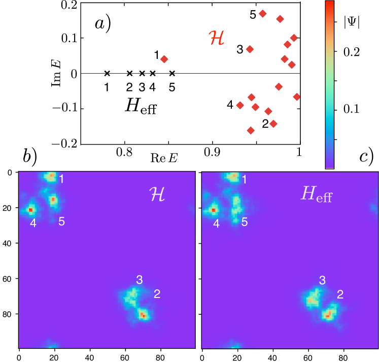
Figure 6: Energy levels (panel a) and localized eigenstates (panels b,c) of the non-Hermitian Hamiltonian ${\cal H}$ from Eq. (17) and its Hermitian counterpart $H_{\rm eff}$ from Eq. (18). The calculations are performed on a 2D square lattice (lattice constant $a\equiv 1$, band width $W_{0}=8$, periodic boundary conditions) for potentials $V_{1}$ and $V_{2}$ randomly and independently chosen at each site, uniformly in the interval $(-1,1)$. A constant offset $V_{0}=1$ was added to $V_{1}$ in order to ensure a positive $V_{\rm eff}$. The mapping from ${\cal H}$ to $H_{\rm eff}$ preserves the spatial location of the localized states, while the ordering of the energy levels $|E_{n}|$ in absolute value is changed. Panels b,c show the eigenstates of the five lowest energy levels of $H_{\rm eff}$ and the corresponding eigenstates of ${\cal H}$. The locations are preserved but $E_{2}$ of ${\cal H}$ is pushed to higher absolute values.

The non-Hermitian Anderson Hamiltonian Tzo19 ; Hua19

$${\cal H}=-\nabla^{2}+V_{1}(\bm{r})+iV_{2}(\bm{r})$$ (17)

has been studied in the context of a random laser Wie08 : a disordered optical lattice with randomly varying absorption and amplication rates, described by a complex dielectric function $V_{1}+iV_{2}$. On a $d$-dimensional square lattice (lattice constant $a$), the discretization of $-\nabla^{2}\mapsto a^{-2}\sum_{i=1}^{d}(2-2\cos k_{i}a)$ produces a spectral band width of $W_{0}=4d/a^{2}$.

The Hermitian Hamiltonian

$$H_{\rm eff}=-\nabla^{2}+V_{\rm eff},\;\;V_{\rm eff}=|\tfrac{1}{2}W_{0}+V_{1}+iV_{2}|-\tfrac{1}{2}W_{0},$$ (18)

is positive-definite if $V_{\rm eff}(\bm{r})>0$ for all $\bm{r}$. The transformation from complex $V$ to real $V_{\rm eff}$ does not change the landscape function, because $\overbracket{\cal H}={\overbracket{H}}_{\rm eff}=H_{\rm eff}$. The localization landscapes are therefore the same and we would expect the eigenstates note3 of ${\cal H}$ and $H_{\rm eff}$ to appear at the same positions, provided that $V_{\rm eff}>0$. This works out, as shown in Fig. 6.

Conclusion and outlook — We have shown that the comparison matrix $\overbracket{H}$ provides a route to the landscape function for Hamiltonians that are not of the Schrödinger form $H=-\nabla^{2}+V$. We have explored Hamiltonians for massive or massless Dirac fermions, with or without superconducting pairing. The broad generality of the approach is highlighted by the application to the non-Hermitian Anderson Hamiltonian.

The localization landscape can be used as a tool to quickly and efficiently find low-lying localized states in a disordered medium, since the landscape function $u(\bm{r})$ is obtained from a single differential equation $\overbracket{H}u=1$. These applications have been demonstrated for the Schrödinger Hamiltonian Fil17 ; Pic17 ; Li17 ; Cha19 , and we anticipate similar applications for the Dirac Hamiltonian in the context of graphene or of topological insulators.

The comparison matrix offers a conceptual insight as well: Since equimodular Hamiltonians have the same comparison matrix, they form an equivalence class that localizes at the same spatial positions. This notion is distinct from the familiar notion of “universality classes” of Anderson localization Eve08 , which refers to ensemble-averaged properties. The equivalence class, instead, refers to sample-specific properties.

As an outlook to future research, it would be interesting to extend the approach from wave functions to energy levels. This has been recently demonstrated for the Schrödinger Hamiltonian Arn19 , where the peak height of the localization function predicts the energy of the localized state. The correlation between peak heights and energy levels evident in Fig. 1 suggests that the comparison matrix has this predictive power as well. Another direction to investigate is to see if the comparison matrix would make it possible to incorporate spin degrees of freedom in the many-body localization landscape introduced recently Bal19 .

Acknowledgements — The 2D numerical calculations were performed using the Kwant code kwant . We have benefited from discussions with I. Adagideli and A. R. Akhmerov. This project has received funding from the Netherlands Organization for Scientific Research (NWO/OCW) and from the European Research Council (ERC) under the European Union’s Horizon 2020 research and innovation programme.

Appendix A Derivation of the comparison inequality

The comparison inequality (4) is derived by Ostrowski Ost37 . Here we give an alternative derivation, to make the paper self-contained.

In the most general case the matrix ${{H}}$ is a complex matrix, not necessarily Hermitian. We will initially assume that the diagonal elements ${{H}}_{nn}$ are real $\geq 0$ and relax that assumption at the end.

Decompose ${{H}}=\lambda\openone-L$, with $\lambda>\max_{n}{{H}}_{nn}$, so that the diagonal elements of $L$ are all positive. If we denote by $|L|$ the elementwise absolute value of the matrix $L$, one has

$$\lambda\openone-|L|=\overbracket{{H}},$$ (19)

under the assumption that ${{H}}_{nn}\geq 0$.

Consider the Euclidean propagator $e^{-{{H}}t}$ for $t\geq 0$, and start from the inequality

$$\left|\textstyle{\sum_{m}}\left(e^{-{{H}}t}\right)_{nm}\Psi_{m}\right|\leq\textstyle{\sum_{m}}\left|\left(e^{-{{H}}t}\right)_{nm}\right||\Psi_{m}|.$$ (20)

We expand $e^{-{{H}}t}$ in a Taylor series,

$$\left|\left(e^{-{{H}}t}\right)_{nm}\right|=e^{-\lambda t}\left|\sum_{p=0}^{\infty}\frac{t^{p}}{p!}(L^{p})_{nm}\right|$$ (21)

$$\leq e^{-\lambda t}\sum_{p=0}^{\infty}\frac{t^{p}}{p!}(|L|^{p})_{nm}=e^{-\lambda t}\bigl{(}e^{|L|t}\bigr{)}_{nm}=\bigl{(}e^{-\overbracket{\scriptstyle{H}}t}\bigr{)}_{nm}.$$

Substitution into Eq. (20) gives

$$\left|\textstyle{\sum_{m}}\left(e^{-{{H}}t}\right)_{nm}\Psi_{m}\right|\leq\textstyle{\sum_{m}}\bigl{(}e^{-\overbracket{\scriptstyle{H}}t}\bigr{)}_{nm}|\Psi_{m}|.$$ (22)

This may also be written more compactly as

$$|e^{-{{H}}t}|\leq e^{-{\overbracket{\scriptstyle{H}}}t},$$ (23)

with the understanding that the absolute value and inequality is taken elementwise.

If we now assume that all eigenvalues of $\overbracket{{H}}$ have a positive real part, then we may integrate both $e^{-{{H}}t}$ and $e^{-\overbracket{\scriptstyle{H}}t}$ over $t$ from 0 to $\infty$. On the one hand we have,

$$\int_{0}^{\infty}e^{-{{H}}t}\,dt={{H}}^{-1},$$ (24)

and on the other hand, in view of Eq. (23), we have

$$\left|\int_{0}^{\infty}e^{-{{H}}t}\,dt\right|\leq\int_{0}^{\infty}|e^{-{{H}}t}|\,dt\leq\int_{0}^{\infty}e^{-\overbracket{\scriptstyle{H}}t}\,dt=\overbracket{{H}}\,^{-1}.$$ (25)

We thus arrive at the desired comparison inequality (4),

$$|{{H}}^{-1}|\leq\overbracket{{H}}\,^{-1}.$$ (26)

The assumption that ${{H}}_{nn}$ is real $\geq 0$ can be removed my multiplying ${{H}}$ with the diagonal matrix

$$D_{nm}=\delta_{nm}\,e^{-i\,{\rm arg}\,{{H}}_{nn}}$$ (27)

(setting $D_{nn}=1$ if ${{H}}_{nn}=0$). This matrix multiplication changes neither the comparison matrix, $\overbracket{D{{H}}}=\overbracket{{H}}$, nor the absolute value of the inverse, $|(D{{H}})^{-1}|=|{{H}}^{-1}D^{-1}|=|{{H}}^{-1}|$, hence Eq. (26) still holds. Only the assumption of positive-definite $\overbracket{H}$ remains.

References

- (1) M. Filoche and S. Mayboroda, Universal mechanism for Anderson and weak localization, PNAS 109, 14761 (2012).
- (2) M. Filoche and S. Mayboroda, The landscape of Anderson localization in a disordered medium, Contemp. Math. 601, 113 (2013).
- (3) D. N. Arnold, G. David, D. Jerison, S. Mayboroda, and M. Filoche, Effective confining potential of quantum states in disordered media, Phys. Rev. Lett. 116, 056602 (2016).
- (4) S. Steinerberger, Localization of quantum states and landscape functions, Proc. Amer. Math. Soc. 145, 2895 (2017).
- (5) M. Filoche, M. Piccardo, Y.-R. Wu, C.-K. Li, C. Weisbuch, and S. Mayboroda, Localization landscape theory of disorder in semiconductors. I. Theory and modeling, Phys. Rev. B 95, 144204 (2017).
- (6) M. Piccardo, C.-K. Li, Y.-R. Wu, J. S. Speck, B. Bonef, R. M. Farrell, M. Filoche, L. Martinelli, J. Peretti, and C. Weisbuch, Localization landscape theory of disorder in semiconductors. II. Urbach tails of disordered quantum well layers, Phys. Rev. B 95, 144205 (2017)
- (7) C.-K. Li, M. Piccardo, L.-S. Lu, S. Mayboroda, L. Martinelli, J. Peretti, J. S. Speck, C. Weisbuch, M. Filoche, and Y.-R. Wu, Localization landscape theory of disorder in semiconductors. III. Application to carrier transport and recombination in light emitting diodes, Phys. Rev. B 95, 144206 (2017).
- (8) Y. Chalopin, F. Piazza, S. Mayboroda, C. Weisbuch, and M. Filoche Universality of fold-encoded localized vibrations in enzymes, arXiv:1902.09939
- (9) D. Arnold, D. Guy, M. Filoche, D. Jerison, and S. Mayboroda, Computing spectra without solving eigenvalue problems, SIAM J. Scientif. Comput. 41, B69 (2019).
- (10) E. M. Harrell II and A. V. Maltsev, Localization and landscape functions on quantum graphs, arXiv:1803.01186.
- (11) C. W. J. Beenakker, Hidden landscape of an Anderson insulator, J. Club Cond. Matt. (August, 2019, DOI).
- (12) A. Ostrowski, Über die Determinanten mit überwiegender Hauptdiagonale, Comment. Mathemat. Helvet. 10, 69 (1937). The comparison inequality is on page 71.
- (13) A. Ostrowski, Determinanten mit überwiegender Hauptdiagonale und die absolute Konvergenz von linearen Iterationsprozessen, Comment. Mathemat. Helvet. 30, 175 (1956).
- (14) Ostrowski originally used the name “companion matrix” (Begleitmatrix), which now refers to a different construction. The notation for the comparison matrix of is common in the mathematical literature, but to avoid confusion with the physics notation for expectation value we use instead. One more piece of nomenclature: If is positive-definite, then it is called an M-matrix while is called an H-matrix.
- (15) For background on comparison matrices, see A. Berham and R. J. Plemmons, Nonnegative Matrices in the Mathematical Sciences (SIAM, 1994).
- (16) The comparison inequality (4) does not require a Hermitian . More generally, if is not Hermitian and has complex eigenvalues the requirement of positive-definiteness is that all eigenvalues have positive real part. We give a general proof of Eq. (4) in the Appendix (supplemental material).
- (17) The discretization (9) is appropriate near the bottom of the tight-binding band at . Near the top of the band at a different discretization produces a different landscape function, as discussed by M. L. Lyra, S. Mayboroda, and M. Filoche, Dual landscapes in Anderson localization on discrete lattices, EPL 109, 47001 (2015).
- (18) A sufficient condition for a positive-definite comparison matrix is that is diagonally dominant, meaning for each . For the Rashba Hamiltonian (10) this implies on a -dimensional square lattice. A necessary and sufficient condition Ber94 for positive-definiteness of is that there exists a vector with positive elements such that for all . For the sufficient condition of diagonal dominance one would take .
- (19) G. Giovannetti, P. A. Khomyakov, G. Brocks, P. J. Kelly, and J. van den Brink, Substrate-induced band gap in graphene on hexagonal boron nitride, Phys. Rev. B 76, 073103 (2007).
- (20) R. Stacey, Eliminating lattice fermion doubling, Phys. Rev. D 26, 468 (1982).
- (21) J. Tworzydło, C. W. Groth, and C. W. J. Beenakker, Finite difference method for transport properties of massless Dirac fermions, Phys. Rev. B 78, 235438 (2008).
- (22) L. Susskind, Lattice fermions, Phys. Rev. D 16, 3031 (1977).
- (23) A. R. Hernández and C. H. Lewenkopf, Finite-difference method for transport of two-dimensional massless Dirac fermions in a ribbon geometry, Phys. Rev. B 86, 155439 (2012).
- (24) The staggered discretization (13) corresponds to the tight-binding Hamiltonian , which gives the dispersion relation (14) when .
- (25) C. W. J. Beenakker and L. P. Kouwenhoven, A road to reality with topological superconductors, Nature Physics 12, 618 (2016).
- (26) N. Read and D. Green, Paired states of fermions in two dimensions with breaking of parity and time-reversal symmetries and the fractional quantum Hall effect, Phys. Rev. B 61, 10267 (2000).
- (27) M. Wimmer, A. R. Akhmerov, M. V. Medvedyeva, J. Tworzydło, and C. W. J. Beenakker, Majorana bound states without vortices in topological superconductors with electrostatic defects, Phys. Rev. Lett. 105, 046803 (2010).
- (28) A. F. Tzortzakakis, K. G. Makris, and E. N. Economou, Non-Hermitian disorder in two-dimensional optical lattices, Phys. Rev. B 101, 014202 (2020).
- (29) Yi Huang and B. I. Shklovskii, Anderson transition in three-dimensional non-Hermitian disorder, arXiv:1911.00562.
- (30) D. S. Wiersma, The physics and applications of random lasers, Nature Phys. 4, 359 (2008).
- (31) Because , the left and right eigenvectors are each others complex conjugate and we do not need to distinguish between these when plotting the absolute value in Fig. 6b.
- (32) F. Evers and A. D. Mirlin, Anderson transitions, Rev. Mod. Phys. 80, 1355 (2008).
- (33) S. Balasubramanian, Y. Liao, and V. Galitski, Many-body localization landscape, Phys. Rev. B 101, 014201 (2020).
- (34) C. W. Groth, M. Wimmer, A. R. Akhmerov, and X. Waintal, Kwant: A software package for quantum transport, New J. Phys. 16, 063065 (2014).