Listen and Fill in the Missing Letters:
Non-Autoregressive Transformer for Speech Recognition

Abstract

Recently very deep transformers have outperformed conventional bi-directional long short-term memory networks by a large margin in speech recognition. However, to put it into production usage, inference computation cost is still a serious concern in real scenarios. In this paper, we study two different non-autoregressive transformer structure for automatic speech recognition (ASR): A-CMLM and A-FMLM. During training, for both frameworks, input tokens fed to the decoder are randomly replaced by special mask tokens. The network is required to predict the tokens corresponding to those mask tokens by taking both unmasked context and input speech into consideration. During inference, we start from all mask tokens and the network iteratively predicts missing tokens based on partial results. We show that this framework can support different decoding strategies, including traditional left-to-right. A new decoding strategy is proposed as an example, which starts from the easiest predictions to the most difficult ones. Results on Mandarin (Aishell) and Japanese (CSJ) ASR benchmarks show the possibility to train such a non-autoregressive network for ASR. Especially in Aishell, the proposed method outperformed the Kaldi ASR system and it matches the performance of the state-of-the-art autoregressive transformer with 7x speedup. Pretrained models and code will be made available after publication.

1 Introduction

In recent studies, very deep end-to-end automatic speech recognition (ASR) starts to be comparable or superior to conventional ASR systems (Karita et al., 2019; Park et al., 2019; Lüscher et al., 2019). They mainly use encoder-decoder structures based on long short-term memory recurrent neural networks (Chorowski et al., 2015; Chan et al., 2016; Watanabe et al., 2018) and transformer networks (Dong et al., 2018; Karita et al., 2019; Lüscher et al., 2019). Those systems have common characteristics: they rely on probabilistic chain-rule based factorization combined with left-to-right training and decoding. During training, the ground truth history tokens are fed to the decoder to predict the next token. During inference, the ground truth history tokens are replaced by previous predictions from the decoder. While this combination allows tractable log-likelihood computation, maximum likelihood training, and beam-search based approximation, it is more difficult to perform parallel computation during decoding. The left-to-right beam search algorithm needs to run decoder computation multiple times which usually depends on output sequence length and beam size. Those models are well-known as auto-regressive models.

Recently, non-autoregressive end-to-end models have started to attract attention in neural machine translation (NMT) (Gu et al., 2017; Lee et al., 2018; Gu et al., 2019; Stern et al., 2019; Welleck et al., 2019; Ghazvininejad et al., 2019). The idea is that the system predicts the whole sequence within a constant number of iterations which does not depend on output sequence length. In (Gu et al., 2017), the author introduced hidden variables denoted as fertilities, which are integers corresponding to the number of words in the target sentence that can be aligned to each word in the source sentence. The fertilities predictor is trained to reproduce the predictions from another external aligner. Lee et al. (2018) used multiple iterations of refinement starting from some “corrupted” predictions. Instead of predicting fertilities for each word in source sequence they only need to predict target sequence total length. Another direction explored in previous studies is to allow the output sequence to grow dynamically (Gu et al., 2019; Stern et al., 2019; Welleck et al., 2019). All those works insert words to output sequence iteratively based on certain order or explicit tree structure. This allows arbitrary output sequence length avoiding deciding before decoding. However since this insertion order or tree structure is not provided as ground truth for training, sampling or approximation is usually introduced to infer it. Among all those studies of different directions, a common procedure for neural machine translation is to perform knowledge distillation (Gu et al., 2017). In machine translation, for a given input sentence, multiple correct translations exist. A pre-trained autoregressive model is used to provide a unique target sequence for training.

Our work is mainly inspired by the conditional language model proposed recently for neural machine translation (Ghazvininejad et al., 2019). Training procedure of this conditional language model is similar to BERT (Devlin et al., 2019). Some random tokens are replaced by a special mask token and the network is trained to predict original tokens. The difference between our approach and BERT is that our system makes predictions conditioned on input speech. Based on observations, we further propose to use factorization loss instead, which bridges the gap between training and inference. During inference, the network decoder can condition on any subsets to predict the rest given input speech. In reality, we start from an empty set (all mask tokens) and gradually complete the whole sequence. The subset we chose can be quite flexible so it makes any decoding order possible. In ASR, there is no need for knowledge distillation since in most cases unique transcript exists.

This paper is organized as follows. Section 2 introduces the autoregressive end-to-end model and section 3 discusses how to adapt it to non-autoregressive. Different decoding strategies are also included. Section 4 introduces the experimental setup and presents results on different corpora. Further analysis is also included discussing the difference between autoregressive and non-autoregressive ASR. Section 5 summarizes this paper and provides several directions for future research in this area.

2 Autoregressive Transformer-based ASR

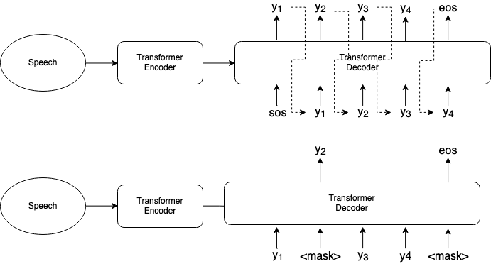
Figure 1: Comparison between normal transformer network and non-autoregressive transformer network. The transformer uses ground truth history tokens during training while during inference previous predictions are used as shown in the dash line. For non-autoregressive transformer training, random tokens in decoder input are replaced by a special $\langle\text{{MASK}}\rangle$token and the network is required to predict for those positions. Both networks conditions on encoder outputs of the whole sequence.

To study non-autoregressive end-to-end ASR, it is important to understand how the current autoregressive speech recognition system works. As shown in Figure 1 top part, general sequence-to-sequence model consists of encoder and decoder. The encoder takes speech features $\mathbf{x}_{t}$ like log Mel filter banks as input and produces hidden representations $\mathbf{h}_{t}$. The decoder predicts a next token $\mathbf{y}_{t}$ based on the previous history $\mathbf{y}_{<t}$ and all hidden representations $\mathbf{h}=(\mathbf{h}_{1},\mathbf{h}_{2},\cdots)$:

$$P(\mathbf{y}_{t}|\mathbf{y}_{<t},\mathbf{x})=P_{\mathsf{dec}}(\mathbf{y}_{t}|\mathbf{y}_{<t},f_{t}(\mathbf{h}))$$ (1)

where $f$ is a $t$-dependent function on all hidden representations $\mathbf{h}$. A common choice for $f$ is an attention mechanism, which can be considered to be a weighted combination of all hidden representations:

$$f^{\mathsf{att}}_{t}(\mathbf{h})=\sum_{t^{{}^{\prime}}}w_{t,t^{{}^{\prime}}}\mathbf{h}_{t^{{}^{\prime}}}$$ (2)

where $t^{{}^{\prime}}$ enumerates all possible hidden representations in $\mathbf{h}$. The weight $w_{t,t^{{}^{\prime}}}$ is usually determined by a similarity between the decoder hidden state at $t$ and hidden representation $\mathbf{h}_{t^{\prime}}$.

During training, the ground truth history tokens $\mathbf{y}_{<t}$ are usually used as input to the decoder in equation 1 for two reasons. First, it is faster since the computation of all $P$ can be performed in parallel, as used in (Vaswani et al., 2017). Second, training can be very difficult and slow if predictions are used instead especially for very long sequence cases (Bengio et al., 2015; Lamb et al., 2016). The expanded computation graph becomes very deep similar to recurrent neural networks without truncating.

During inference, since no ground truth is given, predictions need to be used instead. This means equation (1) needs to be computed sequentially for every token in output and each prediction needs to perform decoder computation once. Depends on output sequence length and unit used, this procedure can be very slow for certain cases, like character-based Transformer models.

3 Non-Autoregressive Transformer-based ASR

Because of the training/inference discrepancy and sequential inference computation, non-autoregressive transformer becomes increasingly popular.

One possibility to make model non-autoregressive is to remove $\mathbf{y}_{<t}$ so parallel computation of $P(\mathbf{y}|\mathbf{h})$ can be factorized as the product of $P(\mathbf{y}_{t}|\mathbf{h})$. However, this conditional independence might be too strong for ASR. Instead, we replace $\mathbf{y}_{<t}$ with some other information like partial decoding results. Similar to previous work (Lee et al., 2018; Ghazvininejad et al., 2019), multiple iterations are adopted to gradually complete prediction of the whole sentence.

3.1 Training Frameworks

3.1.1 Audio-Conditional Masked Language Model (A-CMLM)

One training framework we considered comes from Ghazvininejad et al. (2019). The idea is to replace $\mathbf{y}_{<t}$ with partial decoding results we got from previous computations. A new token $\langle\text{{MASK}}\rangle$is introduced for training and decoding, similar to the idea of BERT (Devlin et al., 2019). Let $T_{\mathrm{M}}$ and $T_{\mathrm{U}}$ be the sets of masked and unmasked tokens respectively. The posterior of the masked tokens given the unmasked tokens and the input speech is,

$$P(\mathbf{y}_{T_{\mathrm{M}}}|\mathbf{y}_{T_{\mathrm{U}}},\mathbf{x})=\prod_{t\in T_{\mathrm{M}}}P_{\mathsf{dec}}(\mathbf{y}_{t}|\mathbf{y}_{T_{\mathrm{U}}},f_{t}(\mathbf{h}))\;.$$ (3)

As shown in Figure 1 bottom part, during training some random tokens are replaced by this special token $\langle\text{{MASK}}\rangle$. The network is asked to predict original unmasked tokens based on input speech and context. The total number of mask tokens is randomly sampled from a uniform distribution of whole utterance length and ground truth tokens are randomly selected to be replaced with this $\langle\text{{MASK}}\rangle$token. Theoretically, if we mask more tokens model will rely more on input speech and if we mask fewer tokens context will be utilized similar to the language model. This combines the advantages of both speech recognition and language modeling. We further assume that given unmasked tokens, predictions of masked tokens are conditionally independent so they can be estimated simultaneously as the product in equation  (3).

ASR uses audio as input (e.g., $f_{t}(\mathbf{h})$ in equation (3)) instead of source text in NMT so we name this as audio-conditional masked language model (A-CMLM).

3.2 Audio-Factorized Masked Language Model (A-FMLM)

During the training of A-CMLM, ground truth tokens at $T_{\mathrm{U}}$ in (3) are provided to predict the masked part. However, during inference none of those tokens are given. Thus the model needs to predict without any context information. This mismatch can be arbitrarily large for some cases, like long utterances from our observations. We will show it in the later experiments.

Inspired by Yang et al. (2019); Dong et al. (2019), we formalize the idea to mitigate the training and inference mismatch as follows. Let $Z_{i}\subset[0,1,...,T-1]$ be a length-$(N+1)$ sequence of indices such that

$$\begin{split}Z_{0}&=\emptyset\\ Z_{N}&=[0,1,...,T-1]\\ \forall i\quad Z_{i}&\subset Z_{i+1}\end{split}$$ (4)

For both training and inference the objective can be expressed as

$$P(\mathbf{y}|\mathbf{h})=\prod_{t=1}^{N}\prod_{i\in Z_{t}\cap{\overline{Z}_{t-1}}}P_{\mathsf{dec}}(\mathbf{y}_{i}|\mathbf{y}_{Z_{t-1}},f_{t}(\mathbf{h}))$$ (5)

where $Z_{t}\cap{\overline{Z}_{t-1}}$ are the indices for decoding in iteration $t$. For example, to decode utterance of length 5 with 5 iterations, one common approach (left to right) can be considered as:

$$\begin{split}Z_{0}&=\emptyset\\ Z_{1}&={0}\\ Z_{2}&={0,1}\\ Z_{3}&={0,1,2}\\ Z_{4}&={0,1,2,3}\\ Z_{5}&={0,1,2,3,4}\\ \end{split}$$ (6)

Here $Z_{t}\cap{\overline{Z}_{t-1}}=t-1$ so in this case equation (5) is equivalent to equation  (1). Similar to A-CMLM, $\langle\text{{MASK}}\rangle$tokens are added to decoder inputs when corresponding tokens are not decided yet. The autoregressive model is a special case when $N=T$ and $Z_{t}=[0,1,...,t]$.

Ideally $Z_{t}$ should be decided based on confidence scores from the network predictions to match inference case. During training we sort all posteriors from iteration $t-1$ and choose those most confident ones. The size of $Z_{t}$ is also sampled from the uniform distribution between $0$ and $T$ to support different possibilities for decoding. To speed-up, we set $N=2$ during training so that optimization objective can be also written as

$$\begin{split}P(\mathbf{y}|\mathbf{h})=&\prod_{i\not\in Z_{1}}P_{\mathsf{dec}}(\mathbf{y}_{i}|\mathbf{y}_{t\in Z_{1}},f_{t}(\mathbf{h}))\\ *&\prod_{j\in Z_{1}}P_{\mathsf{dec}}(\mathbf{y}_{j}|f_{t}(\mathbf{h}))\end{split}$$ (7)

Comparing with equation (3), A-CMLM training only includes first term if $Z_{1}=T_{\mathrm{U}}$. However, during inference, some explicit factorization is still needed.

Pseudo-code of our A-FMLM algorithm can be found in Algorithm 1.

input : minibatch size $n$, dataset D, encoder network $f_{enc}$, decoder network $f_{dec}$

output : Posterior $P$

Sample $x=\mathbf{x}_{1}$, $...$, $\mathbf{x}_{n}$, $y=\mathbf{y}_{1}$, $...$, $\mathbf{y}_{n}$ from D;

$\mathbf{h}=f_{enc}(\mathbf{x})$;

Assign $\langle\text{{MASK}}\rangle$to all elements in $\hat{\mathbf{y}}^{0}$;

$P(\mathbf{y}^{1}|\mathbf{h})=f_{dec}(\hat{\mathbf{y}}^{0},\mathbf{h})$;

$mask=zeros(n,max\_length)$;

Assign $\langle\text{{MASK}}\rangle$to all elements in $\hat{\mathbf{y}}^{1}$;

for i=$1$,$...$,$n$ do

       $probs=P_{i}(\mathbf{y}^{1}|\mathbf{h})$;

       $indices=argsort(probs.max(-1))$;

       $Z\sim Uniform(1,length(probs))$;

       $mask[i,indices[Z:]]=1$;

       $\hat{\mathbf{y}}^{1}[i,indices[Z:]]=y[i,indices[Z:]]$;

      

end for

$P(\mathbf{y}^{2}|\mathbf{h})=f_{dec}(\hat{\mathbf{y}}^{1},\mathbf{h})$;

$P=mask*P(\mathbf{y}^{1}|\mathbf{h})+(1-mask)*P(\mathbf{y}^{2}|\mathbf{h})$;

Algorithm 1 Minibatch forward pass

It is also possible to introduce different networks $P_{\mathsf{dec}}$ for different iterations under our training framework.

3.3 Decoding Strategies

During inference, a multi-iteration process is considered. Other than traditional left-to-right, two different strategies are studied: easy first and mask-predict.

3.3.1 Easy first

The idea of this strategy is to predict the most obvious ones first similar to easy-first parsing introduced in (Goldberg and Elhadad, 2010). In the first iteration, the decoder is fed with predictions $\hat{\mathbf{y}}^{0}_{t}=\text{$\langle\text{{MASK}}\rangle$}$ tokens for all $t$ since we do not have any partial results. After getting decoding results $P(\mathbf{y}^{1}_{t}|.)$, we keep those most confident ones and update them in $\mathbf{y}_{1}$:

$$\hat{\mathbf{y}}^{1}_{t}=\begin{cases}\operatorname*{arg\,max}_{V}P(\mathbf{y}^{1}_{t}|.)&t\in\mathrm{largest}_{C}(\max_{V}P(\mathbf{y}^{1}|.))\\ \hat{\mathbf{y}}^{0}_{t}&\text{otherwise}\end{cases}$$ (8)

where $V$ is the vocabulary, $C=\lceil L/K\rceil$ is the largest number of predictions we keep, $L$ is the sequence length and $K$ is the total number of iterations. Conditioned on this new $\hat{\mathbf{y}}^{1}$, the network is required to make new predictions if there are still masked tokens.

Comparing with Algorithm 1, we used predictions $\operatorname*{arg\,max}_{V}P(\mathbf{y}^{1}_{t}|.)$ instead of ground truth tokens $y[i,indices[Z:]]$.

3.3.2 Mask-predict

This is studied in (Ghazvininejad et al., 2019). Similarly to Section 3.3.1, we start with $\hat{\mathbf{y}}^{0}_{t}=\text{$\langle\text{{MASK}}\rangle$}$. In each iteration $k$, we check the posterior probability of the most probable token for each output $t$ (i.e., $\max_{V}{P(\mathbf{y}^{k}_{t}|.)}$) and use this probability as a confidence score to replace least confident ones in an utterance by $\langle\text{{MASK}}\rangle$tokens. The number of masked tokens in an utterance is $\lceil L*(1-k/K)\rceil$ for $k$-th iteration:

$${\hat{\mathbf{y}}^{k}_{t}=\begin{cases}\text{$\langle\text{{MASK}}\rangle$}&t\in\mathrm{smallest}_{C}(\max_{V}{P(\mathbf{y}_{t}^{k}|.)})\\ \operatorname*{arg\,max}_{V}P(\mathbf{y}^{k}_{t}|.)&\text{otherwise}\end{cases}}$$ (9)

where $C=\lceil L*(1-k/K)\rceil$. For instance, if $K=10$, we mask $90\%$ tokens in the first iteration, $80\%$ in second and so on. After getting prediction results we update all tokens previously masked in $\hat{\mathbf{y}}^{k-1}$:

$$P(\mathbf{y}^{k}_{t}|.)=\begin{cases}P(\mathbf{y}^{k}_{t}|.)&\hat{\mathbf{y}}^{k-1}_{t}=\text{$\langle\text{{MASK}}\rangle$}\\ P(\mathbf{y}^{k-1}_{t}|.)&\text{otherwise}\end{cases}$$ (10)

The difference between mask-predict and easy first is that mask-predict will accept all decisions but it reverts decisions made earlier if it is less confident. Easy first is more conservative and it gradually adopts decisions with the highest confidence. For both strategies, predictions become more and more accurate since it can utilize context information from both future and past directions. This is achieved by replacing input $\mathbf{y}_{<t}$ with all $\mathbf{y}_{t}$ since left-to-right decoding is no longer necessary.

3.4 Example

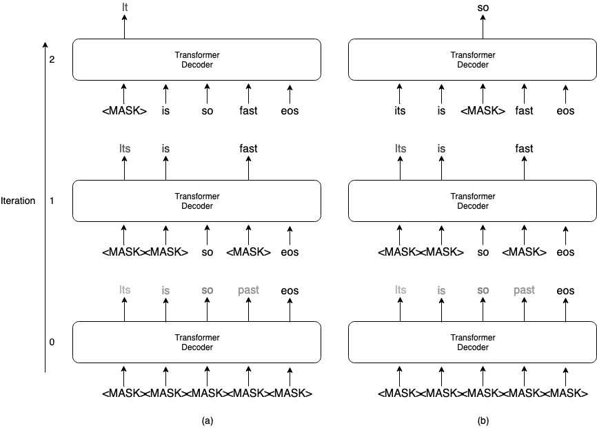
Figure 2: Illustration of inference procedure. To predict the whole sequence with $K=3$ passes, initially, the network is fed with all $\langle\text{{MASK}}\rangle$tokens. Shade here presents the certainties from network outputs. Part (a) shows easy first process. Since token “so” is confident enough in the first iteration to be decided it will never change in the future. Part (b) shows mask-predict process. In the last iteration, it goes back to the word ”so” because it is less confident in the first iteration compared to other predictions in other iterations.

One example is given in Figure 2. Part (a) shows easy first and part (b) demonstrates mask-predict. In this example sequence length is 4 but after adding $\langle\text{{EOS}}\rangle$ token to the end of the sequence we have $L=5$ and $K=3$. In the first iteration, the network is inputted with all $\langle\text{{MASK}}\rangle$. Top $\lceil 5/3\rceil=2$ tokens get kept in each iteration and based on partial results network predicts again on all rest $\langle\text{{MASK}}\rangle$tokens.

For easy first, it always ranks confidence from the last iteration and then keep top-2 confident predictions. Based on partial results it will complete the rest.

For mask-predict it maintains confidence scores from multiple iterations. It chooses the least confident ones from all scores to mask. In the last iteration, it chooses to change its previous prediction of “so” because its confidence is less than other predictions from the second iteration.

Normal inference procedure can be considered as a special case when $K=L$ and instead of taking the most confident one, the prediction of the next token is always adopted. In general, this approach is flexible enough to support different decoding strategies: left-to-right, right-to-left, easy first, mask-predict and other unexplored strategies.

3.5 Output sequence length prediction

In Ghazvininejad et al. (2019) they introduced a special token $\langle\text{{LENGTH}}\rangle$ in input to predict output sequence length. For word sequence this is reasonable but for end-to-end speech recognition, it can be pretty difficult since character or BPE sequence length varies a lot. In this paper a simpler approach is proposed: we asked the network to predict end-of-sequence token $\langle\text{{EOS}}\rangle$ at the end of the sequence as shown in Figure 2.

During inference, we still need to specify the initial length. We manually specify it to some constant value for the first iteration. After that, we change it to the predicted length in the first iteration for speedup.

4 Experiments

For experiments, we mainly use Aishell (Bu et al., 2017) and Corpus of Spontaneous Japanese(CSJ) (Maekawa, 2003). Our preliminary investigations show that a Latin alphabet based task (e.g., English) has some difficulties since the mask-based character prediction in a word is easily filled out only with the character context without using any speech input (i.e., the network only learns the decoder). Although the use of BPE-like sub-words can solve this issue to some extent, this introduces extra complexity and also the non-unique BPE sequence decomposition seems to cause some inconsistency for masked language modeling especially conditioned with the audio input. Due to these reasons, we chose ideogram languages (i.e., Mandarin and Japanese) in our experiments so that the output sequence length is limited and the prediction of the character is enough challenging. Applying the proposed method to the Latin alphabet language is one of our important future work.

ESPnet (Watanabe et al., 2018) is used for all experiments. For the non-autoregressive baseline, we use state-of-the-art transformer end-to-end systems Karita et al. (2019). In Aishell experiments encoder includes 12 transformer blocks with convolutional layers at the beginning for downsampling. The decoder consists of 6 transformer blocks. For all transformer blocks, 4 heads are used for attention. The network is trained for 50 epochs and warmup (Vaswani et al., 2017) is used for early iterations. For all experiments beam search and language model is used and all configuration follows autoregressive baseline.

The results of Aishell is given in Table 1. For A-CMLM, no improvement observed for more than 3 iterations. For A-FMLM, experiments show that 1 iteration is enough to get the best performance. Because of the connection between easy first and A-FMLM, we only use easy first for A-FMLM. All transformer-based experiments are based on pure Python implementation so we don’t compare them with C++-based Kaldi systems in the table. It is still possible to get further speedup by improving current implementation.

All decoding methods result in performance very close to state-of-the-art autoregressive models. Especially A-FMLM matched the performance of autoregressive baseline but real-time factor reduced from 1.44 to 0.22, which is around 7x speedup. The reason is that our non-autoregressive systems only perform decoder computation constant number of times, comparing to the autoregressive model which depends on the length of output sequence. It also outperformed two different hybrid systems in Kaldi by 22% and 11% relative respectively.

System	Dev CER	Test CER	Real Time Factor
Baseline(Transformer)	6.0	6.7	1.44
Baseline(Kaldi nnet3)	-	8.6	-
Baseline(Kaldi chain)	-	7.5	-
An et al. (2019)	-	6.3	-
Fan et al. (2019)	-	6.7	-
Easy first(K=1)	6.8	7.6	0.22
Easy first(K=3)	6.4	7.1	0.22
Mask-predict(K=1)	6.8	7.6	0.22
Mask-predict(K=3)	6.4	7.2	0.24
A-FMLM(K=1)	6.2	6.7	0.28
A-FMLM(K=2)	6.2	6.8	0.22

Table 1: Comparison of baselines, previous work, A-CMLM and A-FMLM on Aishell. For A-CMLM, easy first and mask-predict are compared. For A-FMLM, easy first is utilized since it connects to the factorization used in training.

CSJ results are given in Table 2. Here we observed a larger difference between non-autoregressive models and autoregressive models. Multiple iterations of different decoding strategies are not helping to improve. Still, A-FMLM we proposed outperforms A-CMLM with up to 9x speedup comparing to the autoregressive baseline.

System	Eval1 CER	Eval2 CER	Eval3 CER	Real Time Factor
Baseline(Transformer)	5.9	4.1	4.6	9.50
Baseline(Kaldi)	7.5	6.3	6.9	-
Easy first(K=1)	8.8	6.7	7.4	1.31
Easy first(K=3)	9.3	7.0	8.3	1.05
Mask-predict(K=1)	8.8	6.7	7.4	1.31
Mask-predict(K=3)	11.7	8.8	9.9	1.01
A-FMLM(K=1)	7.7	5.4	6.2	1.40
A-FMLM(K=2)	7.7	5.4	6.2	1.11

Table 2: Comparison of baselines, previous work, A-CMLM and A-FMLM on CSJ. Same systems are compared as above.

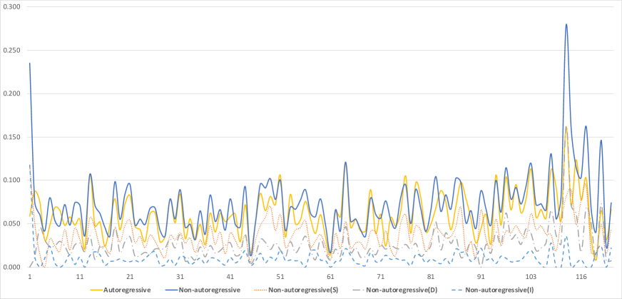
Figure 3: Error analysis of autoregressive and non-autoregressive on different output sequence length. Dash and dot lines indicate different errors: substitute(S), deletion(D), insertion(I)

To understand the performance difference between the autoregressive model and the non-autoregressive model, further analysis is included. In Figure 3 we show the correlation between output sequence length and character error rate for Eval1 set. For short utterances performance of the non-autoregressive model (blue line) is close to the autoregressive model (yellow line). However, when output sequence becomes longer (large than 100), deletion error (long dash-dot line) and substitution error (dot line) start to increase dramatically. This suggests the difficulty of handling very long utterances when the network is trained to predict all tokens simultaneously. More specifically, error rate in the first iteration may increase since it is easy to miss certain token in the long sequence. And those deletion errors increased discrepancy between training and inference which can not be easily fixed because all following tokens need to be moved. This suggests the potential to apply insertion based models like Gu et al. (2019); Stern et al. (2019); Welleck et al. (2019).

5 Conclusion

In this paper, we study two novel non-autoregressive training framework for transformer-based automatic speech recognition (ASR). A-CMLM applies conditional language model proposed in (Ghazvininejad et al., 2019) to speech recognition. Besides decoding strategies like left-to-right, mask-predict, a new decoding strategy is proposed. Based on the connection with a classical dependency parsing (Goldberg and Elhadad, 2010), we named this decoding strategy easy first. Inspired from easy first, we further propose a new training framework: A-FMLM, which utilizes factorization to bridge the gap between training and inference. In experiments, we show that compared to classical left-to-right order these two show great speedup with reasonable performance. Especially on Aishell, the speedup is up to 7 times while performance matches the autoregressive model. We further analyze the problem of the non-autoregressive model for ASR on long output sequences. This suggests several possibilities for future research, e.g., the potential to apply insertion based non-autoregressive transformer model to speech recognition.

References

- An et al. (2019) Keyu An, Hongyu Xiang, and Zhijian Ou. 2019. Cat: Crf-based asr toolkit. arXiv preprint arXiv:1911.08747.
- Bengio et al. (2015) Samy Bengio, Oriol Vinyals, Navdeep Jaitly, and Noam Shazeer. 2015. Scheduled sampling for sequence prediction with recurrent neural networks. In Advances in Neural Information Processing Systems, pages 1171–1179.
- Bu et al. (2017) Hui Bu, Jiayu Du, Xingyu Na, Bengu Wu, and Hao Zheng. 2017. Aishell-1: An open-source mandarin speech corpus and a speech recognition baseline. In 2017 20th Conference of the Oriental Chapter of the International Coordinating Committee on Speech Databases and Speech I/O Systems and Assessment (O-COCOSDA), pages 1–5. IEEE.
- Chan et al. (2016) William Chan, Navdeep Jaitly, Quoc Le, and Oriol Vinyals. 2016. Listen, attend and spell: A neural network for large vocabulary conversational speech recognition. In 2016 IEEE International Conference on Acoustics, Speech and Signal Processing (ICASSP), pages 4960–4964. IEEE.
- Chorowski et al. (2015) Jan K Chorowski, Dzmitry Bahdanau, Dmitriy Serdyuk, Kyunghyun Cho, and Yoshua Bengio. 2015. Attention-based models for speech recognition. In Advances in neural information processing systems, pages 577–585.
- Devlin et al. (2019) Jacob Devlin, Ming-Wei Chang, Kenton Lee, and Kristina Toutanova. 2019. Bert: Pre-training of deep bidirectional transformers for language understanding. In Proceedings of the 2019 Conference of the North American Chapter of the Association for Computational Linguistics: Human Language Technologies, Volume 1 (Long and Short Papers), pages 4171–4186.
- Dong et al. (2019) Li Dong, Nan Yang, Wenhui Wang, Furu Wei, Xiaodong Liu, Yu Wang, Jianfeng Gao, Ming Zhou, and Hsiao-Wuen Hon. 2019. Unified language model pre-training for natural language understanding and generation. arXiv preprint arXiv:1905.03197.
- Dong et al. (2018) Linhao Dong, Shuang Xu, and Bo Xu. 2018. Speech-transformer: a no-recurrence sequence-to-sequence model for speech recognition. In 2018 IEEE International Conference on Acoustics, Speech and Signal Processing (ICASSP), pages 5884–5888. IEEE.
- Fan et al. (2019) Zhiyun Fan, Shiyu Zhou, and Bo Xu. 2019. Unsupervised pre-traing for sequence to sequence speech recognition. arXiv preprint arXiv:1910.12418.
- Ghazvininejad et al. (2019) Marjan Ghazvininejad, Omer Levy, Yinhan Liu, and Luke Zettlemoyer. 2019. Mask-predict: Parallel decoding of conditional masked language models. arXiv preprint arXiv:1904.09324.
- Goldberg and Elhadad (2010) Yoav Goldberg and Michael Elhadad. 2010. An efficient algorithm for easy-first non-directional dependency parsing. In Human Language Technologies: The 2010 Annual Conference of the North American Chapter of the Association for Computational Linguistics, pages 742–750. Association for Computational Linguistics.
- Gu et al. (2017) Jiatao Gu, James Bradbury, Caiming Xiong, Victor OK Li, and Richard Socher. 2017. Non-autoregressive neural machine translation. arXiv preprint arXiv:1711.02281.
- Gu et al. (2019) Jiatao Gu, Qi Liu, and Kyunghyun Cho. 2019. Insertion-based decoding with automatically inferred generation order. arXiv preprint arXiv:1902.01370.
- Karita et al. (2019) Shigeki Karita, Nanxin Chen, Tomoki Hayashi, Takaaki Hori, Hirofumi Inaguma, Ziyan Jiang, Masao Someki, Nelson Enrique Yalta Soplin, Ryuichi Yamamoto, Xiaofei Wang, et al. 2019. A comparative study on transformer vs rnn in speech applications. arXiv preprint arXiv:1909.06317.
- Lamb et al. (2016) Alex M Lamb, Anirudh Goyal Alias Parth Goyal, Ying Zhang, Saizheng Zhang, Aaron C Courville, and Yoshua Bengio. 2016. Professor forcing: A new algorithm for training recurrent networks. In Advances In Neural Information Processing Systems, pages 4601–4609.
- Lee et al. (2018) Jason Lee, Elman Mansimov, and Kyunghyun Cho. 2018. Deterministic non-autoregressive neural sequence modeling by iterative refinement. In Proceedings of the 2018 Conference on Empirical Methods in Natural Language Processing, pages 1173–1182.
- Lüscher et al. (2019) Christoph Lüscher, Eugen Beck, Kazuki Irie, Markus Kitza, Wilfried Michel, Albert Zeyer, Ralf Schlüter, and Hermann Ney. 2019. Rwth asr systems for librispeech: Hybrid vs attention. Interspeech, Graz, Austria, pages 231–235.
- Maekawa (2003) Kikuo Maekawa. 2003. Corpus of spontaneous japanese: Its design and evaluation. In ISCA & IEEE Workshop on Spontaneous Speech Processing and Recognition.
- Park et al. (2019) Daniel S. Park, William Chan, Yu Zhang, Chung-Cheng Chiu, Barret Zoph, Ekin D. Cubuk, and Quoc V. Le. 2019. SpecAugment: A Simple Data Augmentation Method for Automatic Speech Recognition. In Proc. Interspeech 2019, pages 2613–2617.
- Stern et al. (2019) Mitchell Stern, William Chan, Jamie Kiros, and Jakob Uszkoreit. 2019. Insertion transformer: Flexible sequence generation via insertion operations. In International Conference on Machine Learning, pages 5976–5985.
- Vaswani et al. (2017) Ashish Vaswani, Noam Shazeer, Niki Parmar, Jakob Uszkoreit, Llion Jones, Aidan N Gomez, Łukasz Kaiser, and Illia Polosukhin. 2017. Attention is all you need. In Advances in neural information processing systems, pages 5998–6008.
- Watanabe et al. (2018) Shinji Watanabe, Takaaki Hori, Shigeki Karita, Tomoki Hayashi, Jiro Nishitoba, Yuya Unno, Nelson-Enrique Yalta Soplin, Jahn Heymann, Matthew Wiesner, Nanxin Chen, et al. 2018. Espnet: End-to-end speech processing toolkit. Proc. Interspeech 2018, pages 2207–2211.
- Welleck et al. (2019) Sean Welleck, Kianté Brantley, Hal Daumé Iii, and Kyunghyun Cho. 2019. Non-monotonic sequential text generation. In International Conference on Machine Learning, pages 6716–6726.
- Yang et al. (2019) Zhilin Yang, Zihang Dai, Yiming Yang, Jaime Carbonell, Ruslan Salakhutdinov, and Quoc V Le. 2019. Xlnet: Generalized autoregressive pretraining for language understanding. arXiv preprint arXiv:1906.08237.