Tensor methods for the Boltzmann-BGK equation

Abstract

We present a tensor-decomposition method to solve the Boltzmann transport equation (BTE) in the Bhatnagar-Gross-Krook approximation. The method represents the six-dimensional BTE as a set of six one-dimensional problems, which are solved with the alternating least-squares algorithm and the discrete Fourier transform at $N$ collocation points. We use this method to predict the equilibrium distribution (steady-state simulation) and a non-equilibrium distribution returning to the equilibrium (transient simulation). Our numerical experiments demonstrate $N\log N$ scaling. Unlike many BTE-specific numerical techniques, the numerical tensor-decomposition method we propose is a general technique that can be applied to other high-dimensional systems.

2.0pt

1 Introduction

Whenever the mean free path of molecules becomes larger than the characteristic length scale of a system, the continuity assumption breaks down and so does the validity of the Navier-Stokes equations. This phenomenon occurs in a number of settings, including splashing droplets [1], moving contact lines [2], super- and hyper-sonic flows [3], and flow of electrons in metals [4] and silicon [5]. The physics in this flow regime is often described by the six-dimensional (plus time) Boltzmann transport equation (BTE) [6].

Like many other high-dimensional partial differential equations (PDEs), the BTE suffers from the curse of dimensionality: the computational cost of conventional numerical schemes, such as those based on tensor product representations, grows exponentially with an increasing number of degrees of freedom. One way to mitigate such computational complexity is to use particle-based methods [7], e.g., direct simulation Monte Carlo (DSMC) [8] or the Nambu–Babovsky method [9]. These methods preserve the main physical properties of the system, even far from equilibrium, and are computationally efficient away from near-fluid regimes. In particular, they have low memory requirements and their cost scales linearly with the number of particles. However, their accuracy, efficiency and convergence rate tend to be poor for non-stationary flows, or flows close to continuum regimes [10, 11, 12]. This is due to the non-negligible statistical fluctuations associated with finite particle numbers, which are difficult and expensive to filter out in such flow regimes [10, 13]. While several general purpose algorithms have been proposed, the most efficient techniques are problem specific [7, 14, 15, 16]. These methods exploit the BTE’s mathematical properties to arrive at an efficient algorithm, but are not generally applicable to other high-dimensional PDEs.

We present a new algorithm based on tensor decompositions to solve the BTE in the Bhatnagar-Gross-Krook (BGK) approximation [17]. The algorithm relies on canonical tensor expansions [18], combined with either alternating direction least squares methods [19, 20, 21, 22] or alternating direction Galerkin methods [23, 24] or any other version of the method of mean weighted residuals (MWR) [25]. Unlike the BTE-specific numerical techniques, tensor-decomposition methods are general-purpose, i.e., they can be applied to other high-dimensional nonlinear PDEs [26, 27], including but not limited to the Hamilton-Jacobi-Bellman equation [28], the Fokker-Planck equation [29], and the Vlasov equation [30, 31, 32]. This opens the possibility to use tensor methods in many research fields including chemical reaction networks in turbulent flows [33], neuroscience [34], and approximation of functional differential equations [24]. Recently, we developed the tensor-decomposition method [18] to solve a linearized BGK equation. In this paper, we extend it to the full BTE in the BGK approximation, i.e., to obviate the need for the assumption of small fluctuations and to allow for variable density, velocity, temperature, and collision frequency fields.

This paper is organized as follows. Section 2 contains a brief overview of the Boltzmann-BGK equation. In section 3, we propose an efficient algorithm to compute its solution based canonical tensor expansions. Numerical experiments reported in section 4 are used to demonstrate the algorithm’s ability to accurately predict the equilibrium distribution of the system (stead-state), and the exponential relaxation to equilibrium (transient simulation) of non-equilibrium initial states. The algorithm exhibits $\mathcal{O}(N\log(N))$ scaling, where $N$ is the number of degrees of freedom in each of the phase variables. Main conclusions drawn from the numerical experimentation and future directions of research are summarized in section 5.

2 Boltzmann equation

In the classical kinetic theory of rarefied gas dynamics, flow of gases is described in terms of a probability density function (PDF) $f(\mathbf{x},\bm{\xi},t)$, which estimates the number of gas particles with velocity $\bm{\xi}\in\mathbb{R}^{3}$ at position $\mathbf{x}\in\mathbb{R}^{3}$ at time $t\in\mathbb{R}^{+}$, such that $\text{d}N=f\text{d}\mathbf{x}\text{d}\bm{\xi}$ with $N$ denoting the number of particles (in moles). In the absence of external forces, the PDF $f$ satisfies the Boltzmann equation [35],

$$\frac{\partial f}{\partial t}+\bm{\xi}\cdot\nabla_{\mathbf{x}}f=Q(f,f),$$ (1)

where $Q(f,f)$ is the collision integral describing the effects of internal forces due to particle interactions. From the mathematical viewpoint, the collision integral is a functional of the PDF $f$, whose form depends on the microscopic dynamics. For example, in classical rarefied gas flows [36, 37],

$$Q(f,f)(\mathbf{x},\bm{\xi},t)=\int_{\mathbb{R}^{3}}\int_{\mathbb{S}^{2}}B(\bm{\xi},\bm{\xi}_{1},\bm{\omega})\left|f(\mathbf{x},\bm{\xi}^{\prime},t)f(\mathbf{x},\bm{\xi}_{1}^{\prime},t)-f(\mathbf{x},\bm{\xi},t)f(\mathbf{x},\bm{\xi}_{1},t)\right|\text{d}\bm{\omega}\text{d}\bm{\xi}_{1}.$$ (2)

Here, $\bm{\xi}$ and $\bm{\xi}_{1}$ are the velocities of two particles before the collision; $\bm{\xi}^{\prime}=(\bm{\xi}+\bm{\xi}_{1}+\left\|\bm{\xi}-\bm{\xi}_{1}\right\|_{2}\bm{\omega})/2$ and $\bm{\xi}_{1}^{\prime}=(\bm{\xi}+\bm{\xi}_{1}-\left\|\bm{\xi}-\bm{\xi}_{1}\right\|_{2}\bm{\omega})/2$ are these velocities after the collision; $\bm{\omega}$ is the unit vector to the three-dimensional unit sphere $\mathbb{S}^{2}$. The collision kernel $B(\bm{\xi},\bm{\xi}_{1},\bm{\omega})$ is a non-negative function of the Euclidean 2-norm $\left\|\bm{\xi}-\bm{\xi}_{1}\right\|_{2}$ and the scattering angle $\theta$ between the relative velocities before and after the collision,

$$\cos\theta=\frac{(\bm{\xi}-\bm{\xi}_{1})\cdot\bm{\omega}}{\left\|\bm{\xi}-\bm{\xi}_{1}\right\|_{2}}.$$ (3)

Specifically,

$$B(\bm{\xi},\bm{\xi}_{1},\bm{\omega})=\left\|\bm{\xi}-\bm{\xi}_{1}\right\|_{2}\sigma(\left\|\bm{\xi}-\bm{\xi}_{1}\right\|_{2}\cos\theta),$$ (4)

where $\sigma$ is the cross-section scattering function [37]. The collision operator (2) satisfies a system of three conservation laws [7],

$$\int_{\mathbb{R}^{3}}Q(f,f)(\mathbf{x},\bm{\xi},t)\psi(\bm{\xi})\text{d}\bm{\xi}=0,\qquad\text{$\psi(\bm{\xi})=1$ or $\bm{\xi}$ or $\left\|\bm{\xi}\right\|_{2}^{2}$},$$ (5)

for mass, momentum, and energy, respectively. It also satisfies the Boltzmann $H$-theorem,

$$\int_{\mathbb{R}^{3}}Q(f,f)(\mathbf{x},\bm{\xi},t)\log\left(f(\mathbf{x},\bm{\xi},t)\right)\text{d}\bm{\xi}\leq 0,$$ (6)

that implies that any equilibrium PDF, i.e., any PDF $f$ for which $Q(f,f)=0$, is locally Maxwellian:

$$f_{\text{eq}}(\mathbf{x},\bm{\xi},t)=\frac{n(\mathbf{x},t)}{(2\pi k_{\text{B}}T(\mathbf{x},t)/m)^{3/2}}\exp\left(-\frac{m\left\|\mathbf{U}(\mathbf{x},t)-\bm{\xi}\right\|_{2}^{2}}{2k_{\text{B}}T(\mathbf{x},t)}\right).$$ (7)

Here $k_{\text{B}}$ is the Boltzmann constant; $m$ is the particle mass; and the number density $n$, mean velocity $\mathbf{U}$, and temperature $T$ of a gas are defined as

$$n(\mathbf{x},t)= \int_{\mathbb{R}^{3}}f(\mathbf{x},\bm{\xi},t)\text{d}\bm{\xi},$$ (8)

$$\mathbf{U}(\mathbf{x},t)= \frac{1}{n(\mathbf{x},t)}\int_{\mathbb{R}^{3}}\bm{\xi}f(\mathbf{x},\bm{\xi},t)\text{d}\bm{\xi},$$ (9)

$$T(\mathbf{x},t)= \frac{1}{3n(\mathbf{x},t)}\int_{\mathbb{R}^{3}}\left\|\mathbf{U}(\mathbf{x},t)-\bm{\xi}\right\|_{2}^{2}f(\mathbf{x},\bm{\xi},t)\text{d}\bm{\xi}.$$ (10)

The Boltzmann equation (1) is a nonlinear integro-differential equation in six dimensions plus time. By taking suitable averages over small volumes in position space, one can show that the Boltzmann equation is consistent with both the compressible Euler equations [38, 39] and the Navier-Stokes equations [40, 41].

2.1 BGK approximation of the collision operator

The simplest collision operator satisfying the conservation laws (5) and the Boltzmann $H$-theorem (6) is the linear relaxation operator,

$$Q(f,f)=\nu(\mathbf{x},t)\left[f_{\text{eq}}(\mathbf{x},\bm{\xi},t)-f(\mathbf{x},\bm{\xi},t)\right],\qquad\nu(\mathbf{x},t)>0.$$ (11)

It is known as the Bhatnagar-Gross-Krook (BGK) model [17]. The collision frequency $\nu(\mathbf{x},t)$ is usually set to be proportional to the gas number-density and temperature [42],

$$\nu(\mathbf{x},t)=KnT^{1-\mu}.$$ (12)

The exponent of the viscosity law of the gas, $\mu$, depends on the molecular interaction potential and on the type of the gas; and $K=R_{s}T_{\text{ref}}/\mu_{\text{ref}}>0$, where $\mu_{\text{ref}}$ is the gas viscosity at the reference temperature $T_{\text{ref}}$.

The combination of (1) and (11) yields the Boltzmann-BGK equation,

$$\frac{\partial f(\mathbf{x},\bm{\xi},t)}{\partial t}+\bm{\xi}\cdot\nabla_{\mathbf{x}}f(\mathbf{x},\bm{\xi},t)=\nu(\mathbf{x},t)\left[f_{\text{eq}}(\mathbf{x},\bm{\xi},t)-f(\mathbf{x},\bm{\xi},t)\right].$$ (13)

By virtue of (8)–(10), both $f_{\text{eq}}(\mathbf{x},\bm{\xi},t)$ in (7) and $\nu(\mathbf{x},t)$ in (12) are nonlinear functionals of the PDF $f(\mathbf{x},\bm{\xi},t)$. Therefore, (13) is a nonlinear integro-differential PDE in six dimension plus time. It converges to the Euler equations of incompressible fluid dynamics with the scaling $\mathbf{x}^{\prime}=\epsilon\mathbf{x}$ and $t^{\prime}=\epsilon t$, in the limit $\epsilon\rightarrow 0$. However, it does not converge to the Navier-Stokes equations in this limit. Specifically, it predicts an unphysical Prandtl number [43], which is larger than the one obtained with the full collision operator (2). The Navier-Stokes equations can be recovered as $\epsilon$-limits of more sophisticated BGK models, e.g., the Gaussian-BGK model [44].

In previous work [18], we introduced additional simplifications, i.e., assumed $\nu$ to be constant and the equilibrium density, temperature and velocity to be spatially homogeneous. If one additionally assumes $\mathbf{U}\equiv\mathbf{0}$, the resulting model yields an equilibrium PDF $f_{\text{eq}}$ in (7). The last assumption effectively decouples the BGK collision operator from the PDF $f(\mathbf{x},\bm{\xi},t)$. This, in turn, turns the BGK equation into a linear six-dimensional PDE. In this paper, we develop a numerical method to solve the fully nonlinear Boltzmann-BGK equation.

2.2 Scaling

Let us define the Boltzmann-BGK equation (13) on a six-dimensional hypercube, such that $f:\Omega_{\mathbf{x}}\times\Omega_{\bm{\xi}}\times\mathbb{R}^{+}\rightarrow\mathbb{R}^{+}$ with $\Omega_{\mathbf{x}}=[-b_{x},b_{x}]^{3}$ and $\Omega_{\bm{\xi}}=[-b_{\xi},b_{\xi}]^{3}$ representing the spatial domain and the velocity domain, respectively. Furthermore, we impose periodic boundary conditions on all the surfaces of this hypercube. We transform the hypercube $\Omega_{\mathbf{x}}\times\Omega_{\bm{\xi}}$ into the “standard” hypercube $\Omega_{\pi}=[-\pi,\pi]^{6}$, perform simulations in $\Omega_{\pi}$, and then map the numerical results back onto $\Omega_{\mathbf{x}}\times\Omega_{\bm{\xi}}$. This is accomplished by introducing dimensionless independent and dependent variables

$$\tilde{\bm{\xi}}=\frac{\bm{\xi}\pi}{b_{\xi}},\quad\tilde{\mathbf{x}}=\frac{\mathbf{x}\pi}{b_{x}},\quad\tilde{t}=\frac{tb_{\xi}}{b_{x}},\quad\tilde{n}=nb_{x}^{3},\quad\tilde{\mathbf{U}}=\frac{\mathbf{U}\pi}{b_{\xi}},\quad\tilde{T}=\frac{T}{T_{c}},\quad\tilde{\nu}=\frac{\nu\lambda}{b_{\xi}},$$

where $\lambda$ is the mean free path of a gas molecule, and $T_{c}$ is a characteristic temperature. Furthermore, we define the dimensionless Knudsen (Kn) and Boltzmann (Bo) numbers as

$$\text{Kn}=\frac{\lambda}{b_{x}}\quad\text{and}\quad\text{Bo}=\frac{mb_{\xi}^{2}}{\pi^{2}k_{\text{B}}T_{c}}.$$ (14)

Then, the rescaled PDF $\tilde{f}(\tilde{\mathbf{x}},\tilde{\bm{\xi}},\tilde{t})=f(\mathbf{x},\bm{\xi},t)b_{x}^{3}b_{\xi}^{3}/\pi^{3}$ satisfies a dimensionless form of the Boltzmann-BGK equation (13),

$$\frac{\partial\tilde{f}}{\partial\tilde{t}}=L(\tilde{\bm{\xi}})\tilde{f}+C(\tilde{\mathbf{x}},\tilde{\bm{\xi}},\tilde{t}),\qquad L(\tilde{\bm{\xi}})\equiv-\tilde{\bm{\xi}}\cdot\nabla_{\tilde{\mathbf{x}}},\quad C(\tilde{\mathbf{x}},\tilde{\bm{\xi}},\tilde{t})\equiv\frac{\tilde{\nu}}{\text{Kn}}(\tilde{f}_{\text{eq}}-\tilde{f}),$$ (15)

where

$$\tilde{f}_{\text{eq}}(\tilde{\mathbf{x}},\tilde{\bm{\xi}},\tilde{t})=\frac{\tilde{n}}{(2\pi\tilde{T}/\text{Bo})^{3/2}}\exp{\left(-\text{Bo}\frac{\|\tilde{\bm{\xi}}-\tilde{\mathbf{U}}\|^{2}}{2\tilde{T}}\right)},$$ (16)

with

$$\tilde{n}(\tilde{\mathbf{x}},\tilde{t})= \int_{[-\pi,\pi]^{3}}\tilde{f}(\tilde{\mathbf{x}},\tilde{\bm{\xi}},\tilde{t})\text{d}\tilde{\bm{\xi}},$$ (17)

$$\tilde{\mathbf{U}}(\tilde{\mathbf{x}},\tilde{t})= \,\frac{1}{\tilde{n}(\tilde{\mathbf{x}},\tilde{t})}\int_{[-\pi,\pi]^{3}}\tilde{\bm{\xi}}\tilde{f}(\tilde{\mathbf{x}},\tilde{\bm{\xi}},\tilde{t})\text{d}\tilde{\bm{\xi}},$$ (18)

$$\tilde{T}(\tilde{\mathbf{x}},\tilde{t})= \,\frac{\text{Bo}}{3\tilde{n}(\tilde{\mathbf{x}},\tilde{t})}\int_{[-\pi,\pi]^{3}}\|\tilde{\bm{\xi}}-\tilde{\mathbf{U}}(\tilde{\mathbf{x}},\tilde{t})\|_{2}^{2}\tilde{f}(\tilde{\mathbf{x}},\tilde{\bm{\xi}},\tilde{t})\text{d}\tilde{\bm{\xi}}.$$ (19)

For notational convenience, we drop the tilde below, while continuing to use the dimensionless quantities.

3 A tensor method to solve the Boltzmann-BGK equation

Temporal discretization of the Boltzmann-BGK equation (15) is complicated by the presence of the collision term $C(\mathbf{x},\bm{\xi},t)$, whose evaluation is computationally expensive. The combination of the Crank-Nicolson time integration scheme with alternating-direction least squares, implemented in [18], would require multiple evaluations of $C(\mathbf{x},\bm{\xi},t)$ per time step, undermining the efficiency of the resulting algorithm. To ameliorate this problem, we replace the Crank-Nicolson method with the Crank-Nicolson Leap Frog (CNLF) scheme [45, 46, 47, 48]

$$\frac{f(\cdot,t_{n+1})-f(\cdot,t_{n-1})}{2\Delta t}=\frac{L(\bm{\xi})f(\cdot,t_{n+1})+L(\bm{\xi})f(\cdot,t_{n-1})}{2}+C(\cdot,t_{n})+\tau_{n+1},$$ (20)

where $\tau_{n+1}$ is the local truncation error at time $t_{n+1}$.

The CNLF scheme has several advantages over other time-integration methods when applied to tensor discretization of the Boltzmann-BGK equation. First, being an implicit scheme, CNLF allows one to march forward in time by solving systems of linear equations on tensor manifolds with constant rank. Since such manifolds are smooth [50, 51], one can compute these solutions using, e.g., Riemannian quasi-Newton optimization [50, 52, 53] or alternating least squares [19, 54, 55]. Second, CNLF facilitates the explicit calculation of the collision term $C\left(\bm{x},\bm{\xi},t\right)$, and only once per time step. To demonstrate this, we rewrite (20) as

$$\underbrace{[I-\Delta t\,L(\bm{\xi})]}_{A(\bm{\xi})}f(\cdot,t_{n+1})=\underbrace{[1+\Delta t\,L(\bm{\xi})]f(\cdot,t_{n-1})+2\Delta t\,C(\cdot,t_{n})}_{h(\mathbf{x},\bm{\xi},t_{n},t_{n-1})}+2\Delta t\,\tau_{n+1},$$ (21a)

where $$I$$ is the identity operator; or

$$A(\bm{\xi})f(\cdot,t_{n+1})=h(\mathbf{x},\bm{\xi},t_{n},t_{n-1})+2\Delta t\,\tau_{n+1}.$$ (21b)

Given $f(\mathbf{x},\bm{\xi},t_{n})$ and $f(\mathbf{x},\bm{\xi},t_{n-1})$, this equation allows us to compute $f(\mathbf{x},\bm{\xi},t_{n+1})$ by solving a linear system. In the numerical tensor setting described below, this involves only iterations in $f(\mathbf{x},\bm{\xi},t_{n+1})$, which makes it possible to pre-calculate the computationally expensive collision term $C(\mathbf{x},\bm{\xi},t)$ once per time step.

The choice of the time step $\Delta t$ in (21) requires some care, since CNLF is conditionally stable [56]. We transform this scheme into an unconditionally stable one by using, e.g., the Robert-Asselin-Williams (RAW) filter [6, 7, 8].

3.1 Canonical tensor decomposition and alternating least squares (ALS)

We expand the PDF $f(\mathbf{x},\bm{\xi},t_{n})$ in a truncated canonical tensor series [18, 22],

$$f(\mathbf{x},\bm{\xi},t_{n})\simeq\sum_{l=1}^{r_{l}}{f}_{1}^{l}(x_{1},t_{n}){f}_{2}^{l}(x_{2},t_{n}){f}_{3}^{l}(x_{3},t_{n}){f}_{4}^{l}(\xi_{1},t_{n}){f}_{5}^{l}(\xi_{2},t_{n}){f}_{6}^{l}(\xi_{3},t_{n}).$$ (22)

The separation rank $r_{l}$ is chosen adaptively to keep the norm of the residual below a pre-selected threshold at each time $t_{n}$. To simplify the notation, we introduce the combined position-velocity vector $\bm{\zeta}=(\mathbf{x},\bm{\xi})$ and rewrite (22) as

$$f(\bm{\zeta},t_{n})\simeq\sum_{l=1}^{r_{l}}\prod_{k=1}^{6}f_{k}^{l}(\zeta_{k},t_{n}),\qquad\bm{\zeta}\in\Omega_{\pi}=[-\pi,\pi]^{6}.$$ (23)

Next, we expand each function ${f}_{k}^{l}\left(\zeta_{k},t_{n}\right)$ in a finite-dimensional Fourier basis $\phi_{s}(\zeta_{k})$ [60] on $[-\pi,\pi]$,

$$f_{k}^{l}(\zeta_{k},t_{n})=\sum_{s=1}^{Q}\beta_{k,s}^{l}(t_{n})\phi_{s}(\zeta_{k}),$$ (24)

where $Q$ is the number of modes of the Fourier-series expansion, $\beta_{k,s}^{l}\left(t_{n}\right)$ are the (unknown) Fourier coefficients, and $\phi_{s}(\zeta_{k})$ are the orthogonal trigonometric functions. Substituting (23) into (21) yields the residual

$$R(\bm{\zeta},t_{n+1},t_{n},t_{n-1})=\sum_{l=1}^{r_{l}}A\left(\bm{\xi}\right){f}_{1}^{l}\left(\zeta_{1},t_{n+1}\right)\ldots{f}_{6}^{l}\left(\zeta_{6},t_{n+1}\right)-h\left(\bm{\zeta},t_{n},t_{n-1}\right).$$ (25)

The coefficients $\beta_{k,s}^{l}(t_{n})$ are obtained by minimizing the $L^{2}$ norm of this residual with respect to

$$\bm{\beta}(t_{n+1})=[\bm{\beta}_{1}(t_{n+1}),\ldots,\bm{\beta}_{6}(t_{n+1})].$$ (26)

The $k$th vector $\bm{\beta}_{k}(t_{n+1})=[(\beta_{k,1}^{1},\ldots\beta_{k,Q}^{1}),\ldots(\beta_{k,1}^{r},\ldots\beta_{k,Q}^{r})]^{\top}$, for $k=1,\ldots,6$, collects the degrees of freedom representing the PDF $f$ in (23) corresponding to the phase variable $\zeta_{k}$ at time $t_{n+1}$, in accordance with (24).

We employ the alternating least squares (ALS) algorithm [55, 61] to solve the minimization problem

$$\min_{\bm{\beta}_{k}}\left\|R\left(\bm{\zeta},t_{n+1},t_{n},t_{n-1}\right)\right\|^{2}_{L^{2}(\Omega_{\pi})}$$ (27)

sequentially and iteratively for $k=1,\dots,6$. The ALS algorithm is locally equivalent to the linear block Gauss–Seidel iteration method applied to the Hessian of the residual $R$. As a consequence, it converges linearly with the iteration number [54], provided that the Hessian is positive definite (except on a trivial null space associated with the scaling non-uniqueness of the canonical tensor decomposition). Each minimization in (27) yields an Euler-Lagrange equation,

$$\mathbf{M}_{k}(t_{n+1})\bm{\beta}_{k}(t_{n+1})=\bm{\gamma}_{k}(t_{n+1}),\qquad k=1,\dots,6.$$ (28)

Its expanded form reads

$$\underbrace{\left[\!\!\!\!\vphantom{\rule{0.0pt}{88.2037pt}}\begin{array}[]{c@{}c@{}c@{}c}\left[\vphantom{\rule{0.0pt}{27.03003pt}}\begin{array}[]{c@{}c@{}c}(M_{k})_{1,1}^{1,1}&\cdots&(M_{k})_{Q,1}^{1,1}\\ \vdots&\ddots&\vdots\\ (M_{k})_{1,Q}^{1,1}&\cdots&(M_{k})_{Q,Q}^{1,1}\\ \end{array}\right]&\left[\vphantom{\rule{0.0pt}{27.03003pt}}\begin{array}[]{c@{}c@{}c}(M_{k})_{1,1}^{2,1}&\cdots&(M_{k})_{Q,1}^{2,1}\\ \vdots&\ddots&\vdots\\ (M_{k})_{1,Q}^{2,1}&\cdots&(M_{k})_{Q,Q}^{2,1}\end{array}\right]&\cdots&\left[\vphantom{\rule{0.0pt}{27.03003pt}}\begin{array}[]{c@{}c@{}c}(M_{k})_{1,1}^{r,1}&\cdots&(M_{k})_{Q,1}^{r,1}\\ \vdots&\ddots&\vdots\\ (M_{k})_{1,Q}^{r,1}&\cdots&(M_{k})_{Q,Q}^{r,1}\end{array}\right]\\ \left[\vphantom{\rule{0.0pt}{27.03003pt}}\begin{array}[]{c@{}c@{}c}(M_{k})_{1,1}^{1,2}&\cdots&(M_{k})_{Q,1}^{1,2}\\ \vdots&\ddots&\vdots\\ (M_{k})_{1,Q}^{1,2}&\cdots&(M_{k})_{Q,Q}^{1,2}\end{array}\right]&\left[\vphantom{\rule{0.0pt}{27.03003pt}}\begin{array}[]{c@{}c@{}c}(M_{k})_{1,1}^{2,2}&\cdots&(M_{k})_{Q,1}^{2,2}\\ \vdots&\ddots&\vdots\\ (M_{k})_{1,Q}^{2,2}&\cdots&(M_{k})_{Q,Q}^{2,2}\end{array}\right]&\cdots&\left[\vphantom{\rule{0.0pt}{27.03003pt}}\begin{array}[]{c@{}c@{}c}(M_{k})_{1,1}^{r,2}&\cdots&(M_{k})_{Q,1}^{r,2}\\ \vdots&\ddots&\vdots\\ (M_{k})_{1,Q}^{r,2}&\cdots&(M_{k})_{Q,Q}^{r,2}\end{array}\right]\\ \vdots&&\ddots&\vdots\\ \left[\vphantom{\left[\rule{0.0pt}{27.03003pt}\right]}\begin{array}[]{c@{}c@{}c}(M_{k})_{1,1}^{1,r}&\cdots&(M_{k})_{Q,1}^{1,r}\\ \vdots&\ddots&\vdots\\ (M_{k})_{1,Q}^{1,r}&\cdots&(M_{k})_{Q,Q}^{1,r}\end{array}\right]&\left[\vphantom{\left[\rule{0.0pt}{27.03003pt}\right]}\begin{array}[]{c@{}c@{}c}(M_{k})_{1,1}^{2,r}&\cdots&(M_{k})_{Q,1}^{2,r}\\ \vdots&\ddots&\vdots\\ (M_{k})_{1,Q}^{2,r}&\cdots&(M_{k})_{Q,Q}^{2,r}\end{array}\right]&\cdots&\left[\vphantom{\left[\rule{0.0pt}{27.03003pt}\right]}\begin{array}[]{c@{}c@{}c}(M_{k})_{1,1}^{r,r}&\cdots&(M_{k})_{Q,1}^{r,r}\\ \vdots&\ddots&\vdots\\ (M_{k})_{1,Q}^{r,r}&\cdots&(M_{k})_{Q,Q}^{r,r}\end{array}\right]\\ \end{array}\!\!\!\!\right]}_{\mathbf{M}_{k}}\underbrace{\left[\!\!\!\!\vphantom{\rule{0.0pt}{88.2037pt}}\begin{array}[]{c}\left[\vphantom{\rule{0.0pt}{27.03003pt}}\begin{array}[]{c}\beta_{k,1}^{1}\\ \vdots\\ \beta_{k,Q}^{1}\end{array}\right]\\ \left[\vphantom{\rule{0.0pt}{27.03003pt}}\begin{array}[]{c}\beta_{k,1}^{2}\\ \vdots\\ \beta_{k,Q}^{2}\end{array}\right]\\ \vdots\\ \left[\vphantom{\rule{0.0pt}{27.03003pt}}\begin{array}[]{c}\beta_{k,1}^{r}\\ \vdots\\ \beta_{k,Q}^{r}\end{array}\right]\end{array}\!\!\!\!\right]}_{\bm{\beta}_{k}}=\underbrace{\left[\!\!\!\!\vphantom{\rule{0.0pt}{88.2037pt}}\begin{array}[]{c}\left[\vphantom{\rule{0.0pt}{27.03003pt}}\begin{array}[]{c}\gamma_{k,1}^{1}\\ \vdots\\ \gamma_{k,Q}^{1}\end{array}\right]\\ \left[\vphantom{\rule{0.0pt}{27.03003pt}}\begin{array}[]{c}\gamma_{k,1}^{2}\\ \vdots\\ \gamma_{k,Q}^{2}\end{array}\right]\\ \vdots\\ \left[\vphantom{\rule{0.0pt}{27.03003pt}}\begin{array}[]{c}\gamma_{k,1}^{r}\\ \vdots\\ \gamma_{k,Q}^{r}\end{array}\right]\end{array}\!\!\!\!\right]}_{\bm{\gamma}_{k}}$$

where

$$\left(M_{k}\right)_{s,q}^{l,z}(t_{n+1})=\int_{\Omega_{\pi}}\Big{[}A(\bm{\xi})\phi_{s}(\zeta_{k})\prod_{\begin{subarray}{c}j=1\\ j\neq k\end{subarray}}^{6}f_{j}^{l}(\zeta_{j},t_{n+1})\Big{]}\Big{[}A(\bm{\xi})\phi_{q}(\zeta_{k})\prod_{\begin{subarray}{c}j=1\\ j\neq k\end{subarray}}^{6}f_{j}^{z}(\zeta_{j},t_{n+1})\Big{]}\text{d}\bm{\zeta}.$$ (29)

Since the linear operator, first defined in (21), is fully separable (with rank 4), the 6D integral in (29) turns into the sum of the product of 1D integrals. The right hand side of (29) is

$$\gamma_{k,q}^{l}= \int_{\Omega_{\pi}}h(\bm{\zeta},t_{n},t_{n-1})A(\bm{\xi})\phi_{q}(\zeta_{k})\prod_{\begin{subarray}{c}j=1\\ j\neq k\end{subarray}}^{6}f_{j}^{l}(\zeta_{j},t_{n+1})\text{d}\bm{\zeta}$$ (30)

$$= \sum_{m=1}^{r_{m}}\int_{\Omega_{\pi}}\Big{\{}[I+\Delta tL(\bm{\xi})]\prod_{\begin{subarray}{c}j=1\end{subarray}}^{6}f_{j}^{m}(\zeta_{j},t_{n-1})\Big{\}}\Big{\{}A(\bm{\xi})\phi_{q}(\zeta_{k})\prod_{\begin{subarray}{c}j=1\\ j\neq k\end{subarray}}^{6}f_{j}^{l}(\zeta_{j},t_{n+1})\Big{\}}\text{d}\bm{\zeta}$$

$$+2\Delta t\int_{\Omega_{\pi}}C(\bm{\zeta},t_{n})A(\bm{\xi})\phi_{q}(\zeta_{k})\prod_{\begin{subarray}{c}j=1\\ j\neq k\end{subarray}}^{6}f_{j}^{l}(\zeta_{j},t_{n+1})\text{d}\bm{\zeta}.$$

The 6D integrals under the sum are, as before, a sum of the products of 1D integrals, because $L$ is separable with rank 3.

3.2 Evaluation of the BGK collision term

The BGK collision term $C(\bm{\zeta},t_{n})$ in (30),

$$C(\bm{\zeta},t_{n})=\frac{\nu(\mathbf{x},t_{n})}{\text{Kn}}\left[f_{\text{eq}}(\mathbf{x},\bm{\xi},t_{n})-f(\mathbf{x},\bm{\xi},t_{n})\right],$$ (31)

is evaluated by using a canonical tensor decomposition. The equilibrium distribution $f_{\text{eq}}$, defined in (16), is the product of one 3D function and three 4D functions,

$$f_{\text{eq}}(\mathbf{x},\bm{\xi},t_{n})=\frac{n(\bm{x},t_{n})}{[2\pi T(\mathbf{x},t_{n})/\text{Bo}]^{3/2}}\prod_{m=1}^{3}\exp\left(-\text{Bo}\frac{[\xi_{m}-U_{m}(\mathbf{x},t_{n})]^{2}}{2T(\mathbf{x},t_{n})}\right).$$ (32)

Each of these terms are expanded in a canonical tensor series once the number density, velocity and temperature are computed using (17)–(19). The integrals in these expressions are reduced to the products of 1D integrals, once the canonical tensor expansion (23) is available. To calculate the normalization by $n(\mathbf{x},t_{n})$ in (17)–(19) and the normalization by $T(\mathbf{x},t_{n})$ in (32), we employ a Fourier collocation method with $N$ points in each variable. That turns all the integrals into Riemannian sums, and the functions $f_{k}^{l}(\zeta_{k},t_{n})$ into

$$f_{k}^{l}(\zeta_{k,j},t_{n})=\frac{1}{4\pi}\left[\sum_{s=-N/2+1}^{N/2}\beta_{k,s}^{l}\left(t_{n}\right)\text{e}^{is\zeta_{k,j}}+\sum_{s=-N/2}^{N/2-1}\beta_{k,s}^{l}(t_{n})\text{e}^{is\zeta_{k,j}}\right]$$ (33)

with inverse

$$\beta_{k,s}^{l}\left(t_{n}\right)=h\sum_{j=1}^{N}f_{k}^{l}(\zeta_{k,j},t_{n})\text{e}^{-is\zeta_{k,j}}.$$ (34)

Here, $h=2\pi/N$ and $\zeta_{k,j}=-\pi+jh$ with $j=1,\dots,N$. The form of (33) with two different summation intervals is chosen to ensure that the highest wave-number is treated symmetrically [62]. The forward and backward transform is performed efficiently with the Fast Fourier Transform (FFT) and its inverse. The collision frequency $\nu(\mathbf{x},t)=Kn(\mathbf{x},t)T(\mathbf{x},t)^{1-\mu}$ is also represented by a canonical tensor series, once $n(\mathbf{x},t)$ and $T(\mathbf{x},t)$ are available. To speed up the tensor decomposition algorithm, the result from the previous time step is used as the initial guess for the new decomposition.

3.3 Parallel ALS algorithm

Our implementation of the parallel ALS algorithm for solving the Boltzmann transport equation is encapsulated Algorithm 3. The subroutine Initialization initializes all the variables needed to run the code. This includes, initialization of the time-step size $\Delta t$, the number of time steps $n_{\text{max}}$, the number of collocation points, and the initialization of the coefficients $\beta_{\text{New}}$, $\beta_{\text{Now}}$, and $\beta_{\text{Old}}$. These coefficients store, respectively, the values of $f\bm{\zeta},t_{n+1})$, $f(\bm{\zeta},t_{n})$, and $f(\bm{\zeta},t_{n-1})$ in Fourier space. In addition, the operators $A^{+}$, $A^{-}$, and $\text{Exp}_{{A}^{+}}$ are initialized. The operators $A^{+}$ and $A^{-}$ represent $1\pm\Delta t\,L(\bm{\xi})$, respectively. The rank separated operator $\text{Exp}_{{A}^{+}}$ represents operator $A^{+}$ acting on the Fourier basis function $\phi_{s}$. The representation of $A^{+}$ as a single operator reduces the loss of accuracy that comes with multiplying different operators.

Algorithm 1 Parallel ALS algorithm

1:procedure Main

2:     Initialization $\triangleright$ Load variables and allocate matrices

3:     

4:     for $n\leftarrow 1:n_{\text{max}}$ do

5:         $C\leftarrow\textsc{computeArrayC}(\beta_{\text{Now}})$ $\triangleright$ Compute collision operator

6:         

7:         $\beta_{\text{New}}\leftarrow\textsc{randBeta}(\beta_{\text{New}})$ $\triangleright$ Add some random noise

8:         $\epsilon_{|\beta|}\leftarrow\epsilon_{\text{Tol}}+10^{6}$ $\triangleright$ Reset stop criterion

9:         while $\epsilon_{|\beta|}>\epsilon_{\text{Tol}}$ do

10:              $\beta_{\text{Int}}\leftarrow\beta_{\text{New}}$ $\triangleright$ Set intermediate value of beta

11:              

12:              $N\leftarrow\textsc{computeArrayN}(A^{+},A^{-},\text{Exp}_{A^{+}},\beta_{\text{Old}},\beta_{\text{New}})$

13:              $O\leftarrow\textsc{computeArrayO}(C,A^{+},\text{Exp}_{A^{+}},\beta_{\text{New}})$

14:              $\gamma\leftarrow N+2\;\Delta t\;O$

15:              

16:              parfor $d\leftarrow 1:6$ do $\triangleright$ Iterate over dimensions

17:                  $M\left(d\right)\leftarrow\textsc{computeArrayM}(A^{+},\text{Exp}_{A^{+}}\left(d\right),\beta_{\text{New}},d)$               

18:              

19:              parfor $d\leftarrow 1:6$ do

20:                  $\beta_{\text{New}}\left(d\right)\leftarrow\textsc{computeBetaNew}(\beta_{\text{New}}\left(d\right),M\left(d\right),\gamma\left(d\right))$               

21:              

22:              $\beta_{\text{New}}\leftarrow\textsc{kreal}(\beta_{\text{New}})$ $\triangleright$ Keep only real part of solution

23:              $\epsilon_{|\beta|}\leftarrow\textsc{computeNormBeta}(\beta_{\text{Int}},\beta_{\text{New}})$ $\triangleright$ Check for convergence

24:              

25:              if $\epsilon_{|\beta|}>\epsilon_{\text{Tol}}$ then

26:                  $\beta_{\text{New}}\leftarrow\textsc{computeBetaNewDelta}(\beta_{\text{New}},\beta_{\text{Int}})$ $\triangleright$ Update

27:              else

28:                  $\beta_{\text{New}},\beta_{\text{Now}}\leftarrow\textsc{computeRAW}(\beta_{\text{New}},\beta_{\text{Now}},\beta_{\text{Old}})$ $\triangleright$ Apply RAW filter               

29:                       

30:         $\beta_{\text{Old}}=\beta_{\text{Now}}$ $\triangleright$ Update for next time step

31:         $\beta_{\text{Now}}=\beta_{\text{New}}$      

32:end procedure

For every time step, computeArrayC evaluates the BGK collision operator $C(\bm{\zeta},t_{n})$ in (31), and randBeta adds a small amount of noise to $\beta_{\text{New}}$ to prevent the algorithm from getting stuck in a local minimum. The while loop contains the parallel ALS algorithm. The functions computeArrayN and computeArrayO inside the loop compute the two different contributions to the vector $\gamma$ in (30). The function computeArrayM computes the array $M$ inside a parallel for loop, which completes the set of equations (28).

The least-squares routine inside the function computeBetaNew updates $\beta_{\text{New}}$ every iteration inside a parallel for loop. Because of the large number of degrees of freedom in the above system, there are multiple (local minimum) solutions, which are not necessarily real and mass conserving. We ameliorate this problem by adding a constraint that, for every iteration, only the real part of the solution for $\beta_{\text{New}}$ is kept. This calculation is performed by the function kreal. The function computeNormBeta then computes the convergence criterion, $\epsilon_{|\beta|}$, by comparing the current value of $\beta_{\text{New}}$ to its value at the end of the previous iteration, $\beta_{\text{Int}}$. If convergence has not been reached, computeBetaNewDelta updates $\beta_{\text{New}}$ for the next iteration. If convergence has been reached, computeRAW applies the RAW filter [6, 7, 8] to make the CNLF algorithm unconditionally stable, and the algorithm moves on to the next time step.

4 Numerical results

In this section we study the accuracy and computational efficiency of the proposed ALS-CNLF tensor method to solve the Boltzman-BGK equation. (Unless specified otherwise, values of the simulation parameters used in our numerical experiments are collated in Table 1.) We start by validating our solver on a prototype problem involving the Boltzmann-BGK equation in one spatial dimension. Then we consider simulations of the full Boltzmann-BGK equation in three spatial dimensions. The 3D numerical results are split up into steady-state transient problems. The steady-state problem is used to validate the code against an analytical equilibrium solution to the Boltzmann transport equation. It also enables us to investigate the error convergence as function of various parameters, and the code performance as function of the number of collocation points and the number of processor cores. The transient problem starts with an initial distribution away from equilibrium, including a non-zero average velocity in the $x_{1}$ direction, and looks at temporal evolution of the PDF $f$. We compare our code with a spectral code in 2D and present the results for the full 6D Boltzmann-BGK equation.

Variable	Value	Description
$\Delta t$	$0.025$	Dimensionless time step
$K$	$1.0$	Collision frequency pre-factor
$\mu$	$0.5$	Collision frequency temperature exponent
Kn	$1$	Knudsen number
Bo	$3.65$	Boltzmann number
$\epsilon_{\text{Tol}}$	$5.0\cdot 10^{-5}$	Tolerance on ALS iterations

Table 1: Values of parameters used in the simulations of the Boltzmann-BGK equation in three spatial dimensions.

4.1 Transient dynamics in one spatial dimension

To validate the proposed Boltzmann-BGK tensor solver, we first compute the numerical solution of (15) in one spatial dimension, and compare it with an accurate benchmark solution obtained with the high-order Fourier pseudo-spectral method [60]. Specifically, we study the initial-value problem

$$\frac{\partial f(x,\xi,t)}{\partial t}+\xi\frac{\partial f(x,\xi,t)}{\partial x}=\frac{KT(x,t)^{1-\mu}}{\text{Kn}}\left[f_{\text{eq}}(x,\xi,t)-f(x,\xi,t)\right],$$ (35)

$$f\left(x,\xi,0\right)=\frac{n_{0}}{\sqrt{(2\pi T_{0}/\text{Bo})}}\exp{\left(-\frac{\text{Bo}}{2T_{0}}(U_{0}-\xi)^{2}\right)},$$ (36)

with

$$n_{0}=1.0+0.3\cos{(2x)},\qquad U_{0}=1.0+0.1\sin{(3x)},\qquad T_{0}=1.0.$$ (37)

The benchmark numerical solution is constructed by solving (35)–(37) in the periodic box $(x,\xi)\in[-\pi,\pi]^{2}$ with a Fourier pseudo-spectral method [60] (odd expansion on a $61\times 61$ grid) and an explicit two-steps Adams-Bashforth temporal integrator with $\Delta t=0.0005$. The remaining parameters are set to the values from table 1, except $\text{Kn}=10$. Figure 1 exhibits contour plots of the benchmark PDF solution at three times.

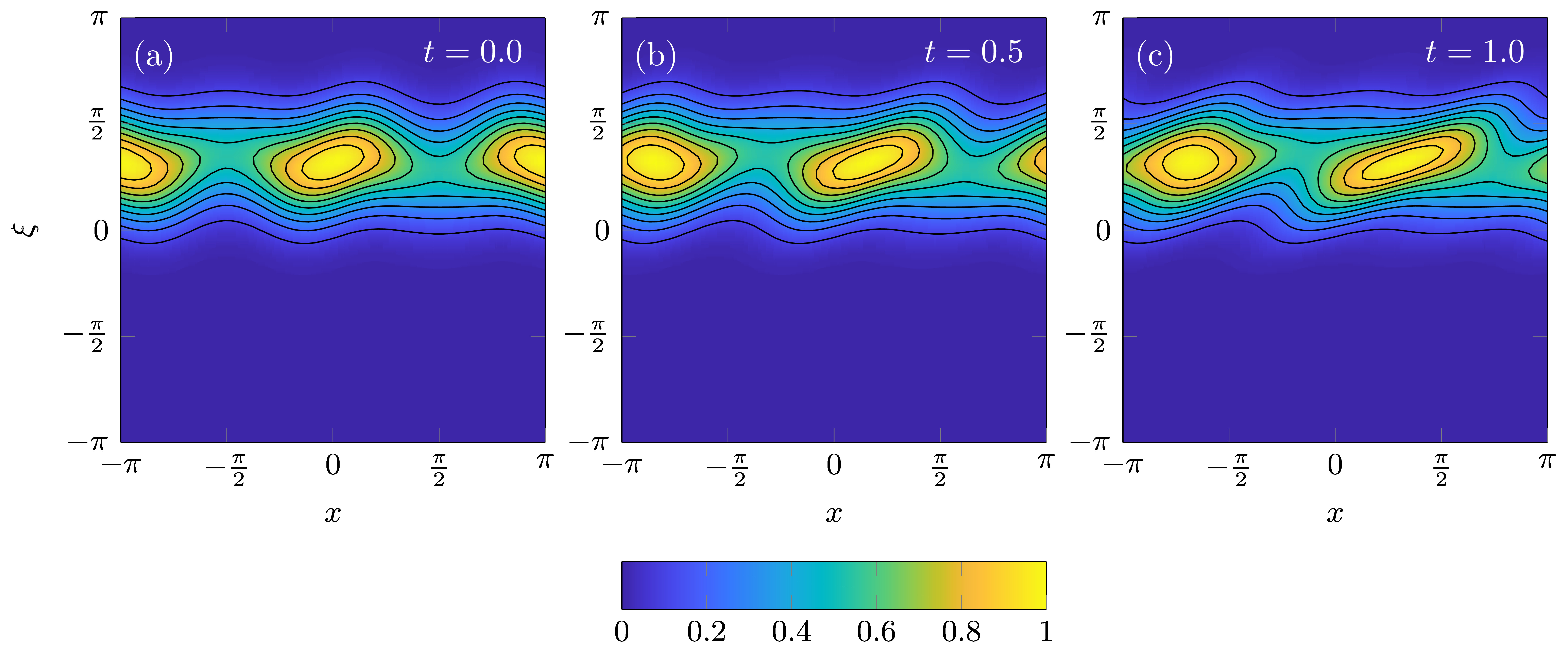
Figure 1: Contour plots of the reference solution to the 1D Boltzmann-BGK initial-value problem (35)–(37), the PDF $f_{\text{spc}}(x,\xi,t)$, computed with the high-order Fourier pseudo-spectral method and explicit two-steps Adams-Bashforth temporal integrator.

We report the accuracy of our ALS-CNLF tensor algorithm by comparing its prediction, $f_{\text{ALS}}$, with the reference solution, $f_{\text{spc}}$, in terms of two metrics. The first is the $L^{2}$ norm

$$\left\|f_{\text{ALS}}(x,\xi,t)-f_{\text{spc}}(x,\xi,t)\right\|=\left(\int_{[-\pi,\pi]^{2}}\left[f_{\text{ALS}}(x,\xi,t)-f_{\text{spc}}(x,\xi,t)\right]^{2}\text{d}x\text{d}\xi\right)^{\!\!1/2}.$$ (38)

The second is the Kullback-Leibler divergence

$$D_{\text{KL}}(F_{\text{ALS}}||F_{\text{spc}})=\int_{[-\pi,\pi]^{2}}f_{\text{ALS}}(x,\xi,t)\log\left[\frac{f_{\text{ALS}}(x,\xi,t)}{f_{\text{spc}}(x,\xi,t)}\right]\text{d}x\text{d}\xi.$$ (39)

In figure 2, we plot these two metrics as function of time $t$ and the tensor rank $r$, which is kept constant throughout the simulation. Bot the $L^{2}$ error and the Kullback-Leibler divergence decrease with the tensor rank $r$.

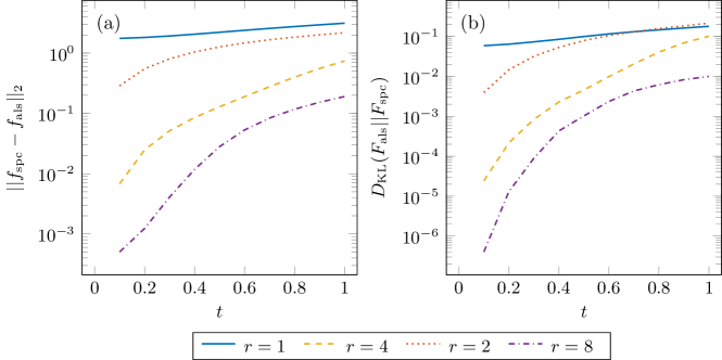
Figure 2: Boltzmann-BGK problem (35)–(37) in one spatial dimension: $L^{2}$ error and Kullback-Leibler divergence of the ALS-CNLF tensor solution, $f_{\text{ALS}}$, relative to the reference solution, $f_{\text{spc}}$, versus time. Both the $L^{2}$ error and the Kullback-Leibler divergence decrease with the tensor rank $r$.

4.2 Steady-state simulations in three spatial dimensions

Since convergence of the ALS algorithm is not guaranteed, e.g., [54, 63], and since the equilibrium distribution is one of the few analytical solutions to the Boltzmann transport equation in six dimensions, we report the code’s behavior at equilibrium. The initial condition in this experiment is the Maxwell-Boltzmann equilibrium PDF, whose moments, as defined in (17)–(19), are set to $n(\mathbf{x},0)=1$, $U_{1}(\mathbf{x},0)=U_{2}(\mathbf{x},0)=U_{3}(\mathbf{x},0)=0$, and $T(\mathbf{x},0)=1$. The simulation was ran till $t=1$. Figure 3 shows temporal variability of the relative errors of the spatial averages, $\left<{n}\right>$ and $\left<{T}\right>$, of the moments $n$ and $T$ and that of the collision frequency, $\left<{\nu}\right>$. Since the initial values of the velocities, $\left<{U_{1}}\right>$, $\left<{U_{2}}\right>$, and $\left<{U_{3}}\right>$, are zero, figure 3b shows only their average values as function of time. For any quantity $a(\mathbf{x},t)$, the spatial average is defined as

$$\left<{a(t)}\right>=\frac{1}{\left(2\pi\right)^{3}}\int_{[-\pi,\pi]^{3}}a(\mathbf{x},t)\text{d}\mathbf{x}.$$ (40)

As expected, all the spatially averaged moments at equilibrium remain approximately constant with time, with small (on the order of $10^{-5}$) deviations representing the numerical error.

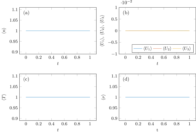
Figure 3: Temporal variability of relative errors in the spatial averages of density, $\left<{n}\right>$, velocity components, $\left<{U_{1}}\right>$, $\left<{U_{2}}\right>$, and $\left<{U_{3}}\right>$, and collision frequency, $\left<{\nu}\right>$, as well as of the spatially averaged temperature, $\left<{T}\right>$. The number of collocation points per dimension is $N=64$. The results show that the code is mass conserving, i.e., the moments of the PDF $f$ at equilibrium are constant constant in time up to a small ($10^{-5}$) error.

Another metric of the accuracy of our steady-state equilibrium solution, the root-mean-square error (RMSE) of the solution is shown in figure 4 as function of time. The RMSE is defined as

$$\text{RMS}(f-f_{0})=\sqrt{\frac{1}{N^{6}}\sum_{i=1}^{N^{6}}(f_{i}-f_{0,i})^{2}},$$ (41)

where $f_{0}$ is the initial condition. The simulation was performed from $N=16$ to $N=64$ collocation points per dimension. However, the number of collocation points does not have a significant effect on the accuracy of the algorithm (figure 4a). Decrease in the time step, from $\Delta t=0.025$ to $\Delta t=0.01$, does not have much effect either. On the other hand, reducing the convergence criterion for $\beta$ from $\epsilon_{\text{Tol}}=5.0\cdot 10^{-5}$ to $\epsilon_{\text{Tol}}=5.0\cdot 10^{-6}$ significantly lowers the error. This suggests the presence of a bottleneck in increasing the accuracy of the simulation caused by the convergence criterion. We show in section 4.3 that the bottleneck for higher accuracy can depend on the physical system.

Since the continuity equation is used as an additional constraint, we explore the behavior of the RMSE of the spatially averaged density $\left<{n}\right>$. Figure 4b shows that our algorithm satisfies mass conservation even at the lowest number of collocation points $N=16$. As the number of collocation points increases from $N=16$ to $N=32$, the error in the mass conservation is significantly reduced. However, the further increase in the number of collocation points, from $N=32$ to $N=64$, hardly has an effect. Also, decreasing the time step from $\Delta t=0.025$ to $\Delta t=0.01$ does not reduce the error. However, as was also observed in figure 4a, reducing the convergence criterion for $\beta$ from $\epsilon_{\text{Tol}}=5.0\cdot 10^{-5}$ to $\epsilon_{\text{Tol}}=5.0\cdot 10^{-6}$ significantly reduces the amount of mass loss. This again confirms that the convergence criterion serves as a bottleneck in increasing the simulation accuracy. This finding highlights the importance of picking a convergence-criterion value that satisfies the desired balance between available computational resources and accuracy. A smaller convergence criterion reduces the error, but results in more iterations to reach convergence and, potentially, in a higher rank of the solution, resulting in higher memory usage.

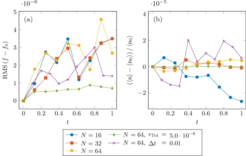
Figure 4: (a) Temporal variability of the RMSE between the computed PDF $f$ and the initial PDF $f_{0}$. Unless otherwise mentioned in the legend $\Delta t=0.025$ and $\epsilon_{\text{Tol}}=5.0\cdot 10^{-5}$. The solution error is relatively independent from the number of collocation points per dimension, $N$. However, reducing the time step $\Delta t$ and, to a larger extent, the convergence criterion $\epsilon_{\text{Tol}}$ significantly reduces the solution error. (b) Mass conservation as function of time $t$. The results show a clear improvement in mass conservation going from $N=16$ to $N=32$, but not from $N=32$ to $N=64$. Decreasing the time step to $\Delta t=0.01$ does not reduce mass loss, while reducing the convergence criterion to $\epsilon_{\text{Tol}}=5.0\cdot 10^{-6}$ significantly improves mass conservation.

The number of iterations, $n_{\beta}$, needed to reach convergence throughout the simulation is reported in figure 5 (the left vertical axis) as function of time $t$. Because the same amount of random noise is added to $\beta$ before starting the ALS algorithm at every time step, the number of iterations is nearly constant. Adding a smaller amount of random noise might reduce the number of iterations, but our numerical experiments revealed that doing so causes the ALS algorithm to get stuck in a local minimum and precludes the residual of the continuity equation, $\epsilon_{|\beta|}$, from being properly minimized. Figure 5 (the right vertical axis) shows that, as the convergence is reached, the difference in the residual between the successive iterations gets smaller. This suggest an exponential decay towards the minimum residual that can be reached before the rank of the solution needs to be increased.

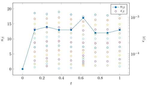
Figure 5: Temporal variability of the umber of iterations, $n_{\beta}$, and convergence, $\epsilon_{|\beta|}$. The number of collocation points per dimension is $N=64$. SInce the same amplitude of random noise to $\beta$ is injected at every time step, the number of iterations is nearly constant in time. The right axis has logarithmic scale, and the distance between each iteration decreases as convergence is reached. This suggest that convergence follows an exponential decay.

The computational efficiency of our code is reported in figure 6. The left frame shows the scaling of the wall time, $t_{\text{Wall}}$, with the number of collocation points per dimension, $N$, on one CPU core. The performance of the code is close to $N\log{\left(N\right)}$ in the range of the explored collocation points. The most time is spent in the LSQR [64] subroutine, which is used to implicitly solve for $\beta$ for each dimension during every iteration of the ALS procedure. This suggest that the code could be further optimized by replacing the existing LSQR algorithm with its more efficient implementation, e.g., [65]. The right frame of figure 6 exhibits the scaling of the wall time, $t_{\text{Wall}}$, with the number of processors, $n_{\text{Proc}}$. The curve $1/n_{\text{Proc}}$ represents the ideal scaling without any communication overhead. Even though the different dimensions can all be solved for independently, the scaling of our code with the number of processors is quite poor. This suggests that the code can be optimized further by minimizing the communication between different CPU cores. One way to approach this would be to rewrite the code around a specialized parallel processing MPI library and have finer control over both data communication between processor cores and protocol selection.

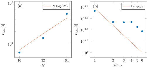
Figure 6: Scaling of the wall time $t_{\text{Wall}}$ with (a) the number of collocation points per dimension, $N$, and (b) the number of processors, $n_{\text{Proc}}$. The calculations to determine the scaling of the wall time as function of the number of collocation points were performed on a single core.

4.3 Relaxation to statistical equilibrium in three spatial dimensions

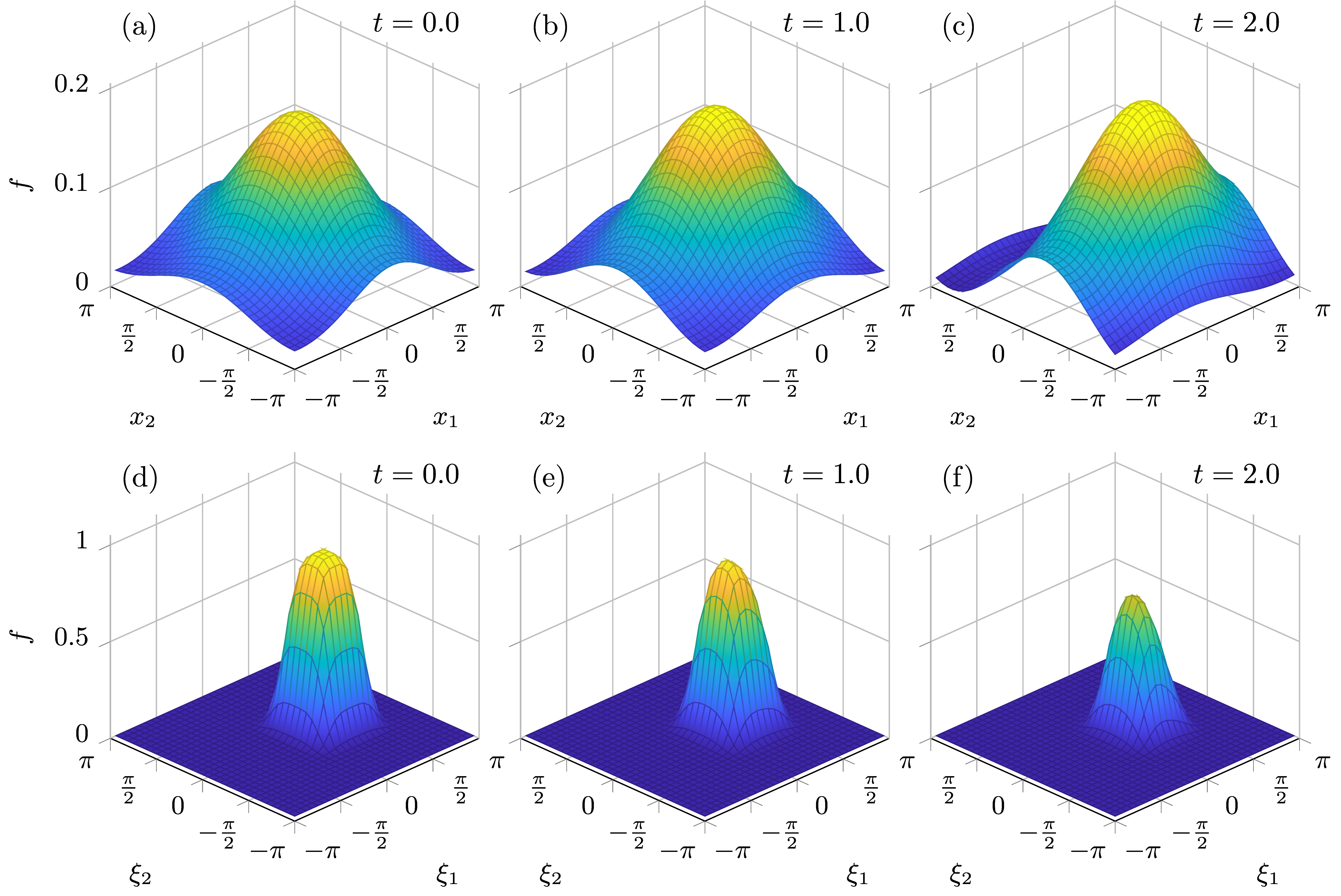
Figure 7: Temporal evolution of the PDF $f(\mathbf{x},\bm{\xi},t)$ in hyper-planes $(\mathbf{x};\bm{\xi})=(x_{1},x_{2},0;\mathbf{0})$ (top row) and $(\mathbf{0};\xi_{1},\xi_{2},0)$ (bottom row). The number of collocation points per dimension is $N=32$. The color-coding is consistent among the different frames in a row. The PDF $f$ evolves from its initial, far-from-equilibrium state (42) towards its equilibrium state (16).

In this section, we study relaxation to statistical equilibrium predicted by the dimensionless Boltzmann-BGK model (15)–(19), subject to the initial condition

$$f(\mathbf{x},\bm{\xi},0)=Wf_{1}(x_{1},\xi_{1},0)f_{2}(x_{2},\xi_{2},0)f_{3}(x_{3},\xi_{3},0)$$ (42a)

with

$$f_{i}(x_{i},\xi_{i},0) =\frac{\sqrt[3]{n_{0}}}{\sqrt{2\pi T_{0}/\text{Bo}}}\exp\left[-\frac{\text{Bo}}{2T_{0}}(U_{i,0}-\xi_{i})^{4}\right],\qquad i=1,2,3$$ (42b)

and $n_{0}=\prod_{i=1}^{3}(0.5\cos x_{i}+1)$, $T_{0}=0.0025\cos(x_{1})$, $U_{1,0}=1+0.025\sin(x_{2}-1)$, $U_{2,0}=0$, and $U_{3,0}=0.025\sin(x_{1}-2)$. The integral over the PDF is normalized to 1 by computing the value of $W$. The difference between the initial PDF and the local equilibrium PDF causes the Boltzmann equation to evolve while the fluctuations in the initial fields are introduced to show the code’s ability to operate away from global equilibrium. In this experiment, the Knudsen number is set to $\text{Kn}=10$. Figure 7 shows the PDF $f(\mathbf{x},\bm{\xi},t)$ in the ($x_{1}$-$x_{2}$) and ($\xi_{1}$-$\xi_{2}$) hyper-planes. The PDF $f$ evolves from its initial state far from equilibrium to the equilibrium Maxwell-Boltzmann PDF $f_{\text{eq}}$. Figure 8 further elucidates this dynamics by exhibiting temporal snapshots of the PDF $f(\mathbf{x},\bm{\xi},t)$ in hyper-planes $(\mathbf{x};\bm{\xi})=(x_{1},0,0;\mathbf{0})$, $(0,x_{2},0;\mathbf{0})$, $(0,0,x_{3};\mathbf{0})$, $(\mathbf{0};\xi_{1},0,0)$, $(\mathbf{0};0,\xi_{2},0)$, and $(\mathbf{0};0,0,\xi_{3})$.

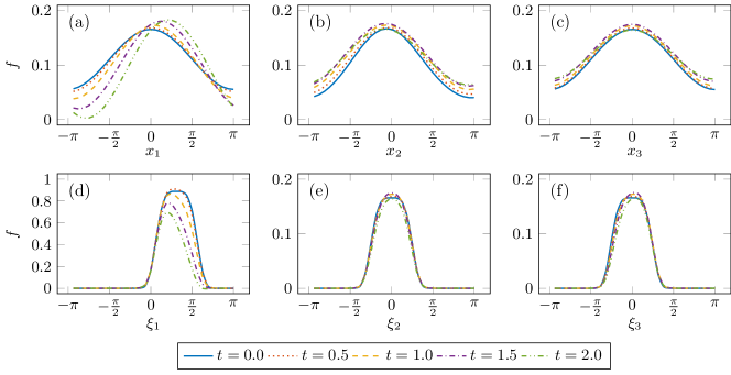
Figure 8: Temporal evolution of the PDF $f(\mathbf{x},\bm{\xi},t)$ in hyper-planes (a) $(\mathbf{x};\bm{\xi})=(x_{1},0,0;\mathbf{0})$, (b) $(\mathbf{x};\bm{\xi})=(0,x_{2},0;\mathbf{0})$, (c) $(\mathbf{x};\bm{\xi})=(0,0,x_{3};\mathbf{0})$, (d) $(\mathbf{x};\bm{\xi})=(\mathbf{0};\xi_{1},0,0)$, (e) $(\mathbf{x};\bm{\xi})=(\mathbf{0};0,\xi_{2},0)$, and (f) $(\mathbf{x};\bm{\xi})=(\mathbf{0};0,0,\xi_{3})$. The number of collocation points per dimension is $N=32$. The PDF $f$ evolves from its initial, far-from-equilibrium state (42) towards its equilibrium state (16).

Finally, figure 9 exhibits temporal evolution of the number density $n(\mathbf{x},t)$, velocity $\mathbf{U}(\mathbf{x},t)$, temperature $T(\mathbf{x},t)$, and the collision frequency $\nu(\mathbf{x},t)$, all evaluated at the hyper-plane $\mathbf{x}=(x_{1},0,0)$. As expected, the magnitude of the velocity components $U_{2}$ and $U_{3}$ is about $100$ times smaller than that of the $U_{1}$ component (frames a–c). The effect of the flow in the $x_{1}$ direction is seen in frame (d), where the density profile shifts to the right as time progresses; in addition, the height of the density profile decreases as the mass is redistributed by diffusion. While not discernible from these figures, the code does suffer from a small amount of mass loss of about $2\%$ per unit time. This is most likely due to a combination of small truncation errors, convergence tolerances, and time step size. Frame (e) shows evolution of the temperature $T(x_{1},\cdot,t)$ from its initial nearly uniform state. Increasing velocity fluctuations drive the increase in temperature fluctuations. The collision frequency (frame f) is computed directly from the density and temperature fields according to 12. Overall all, the PDF and its moments show the expected physical behavior and evolve towards the equilibrium Maxwell-Boltzmann distribution.

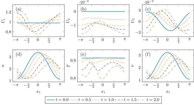
Figure 9: Temporal evolution of (a–c) the velocity components $U_{i}\mathbf{x},t)$, (d) number density $n(\mathbf{x},t)$, (e) temperature $T(\mathbf{x},t)$, and (f) the collision frequency $\nu(\mathbf{x},t)$, all evaluated at the hyper-plane $\mathbf{x}=(x_{1},0,0)$. The number of collocation points per dimension is $N=32$.

5 Discussion and conclusions

We demonstrated the ability of canonical polyadic tensor decomposition to solve the BGK approximation of the six-dimensional Boltzmann transport equation with variable density, velocity, temperature, and collision frequency fields. This extends the usage of this method from only fully separable differential operators, to partially separable operators. The dependent variables in the Boltzmann equation are computed via the pseudo-spectral method with collocation points. The different dimensions are solved using a parallel ALS algorithm. Our numerical experiments show that the code is capable of simulating both a system’s steady state and its temporal evolution starting from a state far away from equilibrium. The highest simulation accuracy is achieved by identifying a correct bottleneck: in the steady-state simulations the limiting factor is the convergence tolerance. The code’s performance scales as $N\log(N)$ with the number of collocation points per dimension, $N$.

In future work, we will further optimize the code, implement different boundary conditions, and explore the feasibility of using the code with other collision operators. Significant speedup can be achieved by rank reduction of the collision operator. The currently used reconstruction of the collision operator via multiplication of its different components can result in a high-rank operator, which can become degenerate. Reducing the rank of this tensor, while maintaining accuracy, is a topic that needs further study. Another aspect where the code can be improved is parallelization, especially when using the CNLF-ALS method to solve problems of dimensionality higher than that of the Boltzmann-BGK equation. One way to approach this would be to rewrite the code around a specialized parallel processing MPI library and have finer control over data communication between processor cores and protocol selection.

Generalizations to other types of boundary conditions would require an in-depth investigation of the trial function behavior. The choice of a right trial function for a certain system is typically determined by one of the two approaches. First, one selects a trial function that obeys the desired boundary conditions and then sums over the trial functions to reconstruct the solution to a PDE. Second, one selects a trial function that captures the PDE solution and then adds trial functions to reconstruct the boundary condition. Figure 8 shows that the six-dimensional Boltzmann equation subject to periodic boundary conditions can be efficiently solved by using the discrete Fourier series. The presence of, e.g., a wall would introduce the Maxwell boundary condition [35, 66]. The latter consists of two parts: one represents the reflection of particles from the wall and the other represents absorption and emission of particles on the wall. Since there is no known trial function to either solve the Boltzmann equation in the bulk or the Maxwell boundary condition on the wall, another method of the trial-function selection is needed. Such methods include the tau method [67], the penalty approach [68], and the mixed method [69, 70, 71]. They have been used to implement boundary condition for the weighted residuals and spectral methods [72, 68], but have not yet been applied in the tensor decomposition setting.

While the boundary conditions are very important for engineering applications, some fundamental questions remain to be resolved as well. The empirical evidence shows convergence the tensor algorithms, but its theoretical proof is lacking. That is largely due to two factors. First, it is generally assumed that increasing the rank of the solution improves its accuracy and in, some cases, tensor decomposition was shown to be exponentially more efficient than one would expect a priori [22]. However, there is no mathematical proof which indicates how high the rank needs to be to reach a certain accuracy and how fast the solution converges as a function of its rank. This question is very important for the speed of tensor decomposition, because the higher the rank of the operators and the solution of the Boltzmann equation, the slower the computation becomes. Second, from one time step to the next convergence is not guaranteed. The ALS method implemented in our code is a variation on the Gauss-Seidel method whose convergence can be proven for some specific cases [54]. However, only the Jacobi method can decouple the different dimensions and parallelize the algorithm. How the adoption of this method would change convergence remains to be investigated.

Acknowledgements This research was supported in part by the U.S. Army Research Office (ARO) grant W911NF1810309 awarded to Daniele Venturi, and by the Air Force Office of Scientific Research (AFOSR) grant FA9550-18-1-0474 awarded to Daniel Tartakovsky.

Equations (15)–(19) are solved with a Matlab [1] code that uses the Matlab Tensor Toolbox [2]. One of the core elements of the code is a special case of the Tucker operator, the so-called “Kruskal operator” [3, 4]. In three dimensions this operator is defined as

$$a_{i,j,k}=\sum_{r_{a}=1}^{R_{a}}\lambda_{r_{a}}\;a_{1,i,r_{a}}\;a_{2,j,r_{a}}\;a_{3,k,r_{a}}\text{ for all $i,j,k$},$$ (S1)

where $R_{a}$ is the rank of the operator. In general, $\lambda_{r}$ is used as a prefactor to normalize the matrices $a_{1,i,r},\dots,a_{6,n,r}$, but in our code $\lambda_{r}=1$ for simplicity. The code uses a number of basic operations: the mtimesk subroutine of Algorithm 2 performs simple multiplication of two Kruskal operators $a_{i,j,k}$ and $b_{i,j,k}$. For example, for all $i,j,k$,

$$\textsc{mtimesk}\left(a_{i,j,k},b_{i,j,k}\right)=\sum_{r_{a}=1}^{R_{a}}\sum_{r_{b}=1}^{R_{b}}\lambda_{r_{a}}\lambda_{r_{b}}\;a_{1,i,r_{a}}b_{1,i,r_{b}}\;a_{2,j,r_{a}}b_{2,j,r_{b}}\;a_{3,k,r_{a}}b_{3,k,r_{b}},$$ (S2)

creating a new Kruskal operator of rank $R=R_{a}R_{b}$. The mtimeskBlock subroutine also performs multiplication but does so in blocks. In the case of $2\times 2$ blocks of length $R_{a}^{\prime}$ and $R_{b}^{\prime}$,

$$\textsc{mtimeskBlock}\left(a_{i,j,k},b_{i,j,k},R_{a},R_{b},R_{a}^{\prime},R_{b}^{\prime}\right)=\\ \begin{aligned} &\sum_{r_{a}=1}^{R_{a}^{\prime}}\sum_{r_{b}=1}^{R_{b}^{\prime}}\lambda_{r_{a}}\lambda_{r_{b}}\;a_{1,i,r_{a}}b_{1,i,r_{b}}\;a_{2,j,r_{a}}b_{2,j,r_{b}}\;a_{3,k,r_{a}}b_{3,k,r_{b}}\\ +&\sum_{r_{a}=1}^{R_{a}^{\prime}}\sum_{r_{b}=R_{b}^{\prime}+1}^{R_{b}}\lambda_{r_{a}}\lambda_{r_{b}}\;a_{1,i,r_{a}}b_{1,i,r_{b}}\;a_{2,j,r_{a}}b_{2,j,r_{b}}\;a_{3,k,r_{a}}b_{3,k,r_{b}}\\ +&\sum_{r_{a}=R_{a}^{\prime}+1}^{R_{a}}\sum_{r_{b}=1}^{R_{b}^{\prime}}\lambda_{r_{a}}\lambda_{r_{b}}\;a_{1,i,r_{a}}b_{1,i,r_{b}}\;a_{2,j,r_{a}}b_{2,j,r_{b}}\;a_{3,k,r_{a}}b_{3,k,r_{b}}\\ +&\sum_{r_{a}=R_{a}^{\prime}+1}^{R_{a}}\sum_{r_{b}=R_{b}^{\prime}+1}^{R_{b}}\lambda_{r_{a}}\lambda_{r_{b}}\;a_{1,i,r_{a}}b_{1,i,r_{b}}\;a_{2,j,r_{a}}b_{2,j,r_{b}}\;a_{3,k,r_{a}}b_{3,k,r_{b}}\text{ for all $i,j,k$}.\end{aligned}$$ (S3)

The subroutines krepmat and krepelem repeat the whole Kruskal object or its individual elements, respectively. For instance, for all $i,j,k$,

$$\textsc{krepmat}\left(a_{i,j,k},2\right)=\sum_{r_{a}=1}^{R_{a}}\lambda_{r_{a}}\;a_{1,i,r_{a}}\;a_{2,j,r_{a}}\;a_{3,k,r_{a}}+\sum_{r_{a}=1}^{R_{a}}\lambda_{r_{a}}\;a_{1,i,r_{a}}\;a_{2,j,r_{a}}\;a_{3,k,r_{a}}$$ (S4)

and

$$\textsc{krepelem}\left(a_{i,j,k},2\right)=\sum_{r_{a}=1}^{R_{a}}\lambda_{r_{a}}\;a_{1,i,r_{a}}\;a_{2,j,r_{a}}\;a_{3,k,r_{a}}+\lambda_{r_{a}}\;a_{1,i,r_{a}}\;a_{2,j,r_{a}}\;a_{3,k,r_{a}}.$$ (S5)

The kreshape subroutine extends a Kruskal operator to a higher dimension. To add the fourth dimension to $a_{i,j,k}$, one writes

$$\textsc{kreshape}\left(a_{i,j,k},[1\;1\;0\;1]\right)=\sum_{r_{a}=1}^{R_{a}}\lambda_{r_{a}}\;a_{1,i,r_{a}}\;a_{2,j,r_{a}}\;b_{1,l,r_{a}}\;a_{3,k,r_{a}},\quad\text{ for all $i,j,k,l$}.$$ (S6)

In this example, $a_{3,k,r_{a}}$ becomes the fourth dimension and the third dimension equals $b_{1,l,r_{a}}=1$ for all values of $l$ and $r_{a}$.

Algorithm 2 computeG subroutine

1:function computeG($A,\beta,R,R_{\text{Exp}}$)

2:     

3:     $\beta\leftarrow\textsc{krepelem}(\beta,R_{\text{Exp}})$ $\triangleright$ Repeat elements of beta

4:     

5:     $\beta\leftarrow\textsc{computeF}(\beta,[0\;0\;0\;1\;1\;1])$ $\triangleright$ iFFT where A works in real space

6:     

7:     $\beta\leftarrow\textsc{mtimeskBlock}(A,\beta,R_{\text{A}},R,1,R_{\text{Exp}})$ $\triangleright$ Apply operator A

8:     

9:     $G\leftarrow\textsc{computeF}(\beta,[1\;1\;1\;0\;0\;0])$ $\triangleright$ iFFT where A works in Fourier space

10:     

11:     return $G$

12:end function

Algorithm 3 shows the Parallel Alternating Least Squares (ALS) algorithm used to solve the Boltzmann transport equation. The subroutine Initialization initializes all variables to run the code. This includes variables like the ones listed in table 1, but also the operators $A$, $A^{+}$, $A^{-}$, Exp, $\text{Exp}_{A}$, and $\text{Exp}_{{A}^{+}}$. The operators $A$, $A^{+}$, and $A^{-}$ are the respective Kruskal operator representations of the operators introduced in section 3.3. For these operators, multiplication with $\xi_{k}$ is represented in real space and derivatives are represented in Fourier space to achieve spectral accuracy. This means that to apply these operators to a function, the velocity space, i.e., the first three dimensions, of this function have to be in physical space and the velocity space, i.e., the last three dimensions, have to be in Fourier space. This can be seen in the computeG subroutine in Algorithm 2 that is used throughout the code.

Algorithm 3 Parallel Alternating Least Squares (ALS) algorithm

1:procedure Main

2:     Initialization $\triangleright$ Load variables and allocate matrices

3:     $\beta_{\text{New}}=\beta_{\text{Now},0}$ $\triangleright$ Set initial condition

4:     $\beta_{\text{Now}}=\beta_{\text{Now},0}$

5:     $\beta_{\text{Old}}=\beta_{\text{Old},0}$

6:     

7:     for $n\leftarrow 1:n_{\text{max}}$ do

8:         $C\leftarrow\textsc{computeArrayC}(\beta_{\text{Now}})$ $\triangleright$ Compute collision operator

9:         

10:         $\beta_{\text{New}}\leftarrow\textsc{randBeta}(\beta_{\text{New}})$ $\triangleright$ Add some random noise

11:         $\epsilon_{|\beta|}\leftarrow\epsilon_{\text{Tol}}+10^{6}$ $\triangleright$ Reset stop criterion

12:         while $\epsilon_{|\beta|}>\epsilon_{\text{Tol}}$ do

13:              $\beta_{\text{Int}}\leftarrow\beta_{\text{New}}$ $\triangleright$ Set intermediate value of beta

14:              

15:              $N_{0}\leftarrow\textsc{computeArrayN0}(A^{+},A^{-},\text{Exp}_{A^{+}},\beta_{\text{Old}},\beta_{\text{New}})$

16:              $O_{0}\leftarrow\textsc{computeArrayO0}(C,A^{+},\text{Exp}_{A^{+}},\beta_{\text{New}})$

17:              $\gamma_{0}\leftarrow N_{0}+2\;\Delta t\;O_{0}$

18:              

19:              $\gamma_{1}\leftarrow\textsc{computeArrayN1}(\text{Exp},A,\text{Exp}_{A},\beta_{\text{Now}},\beta_{\text{New}})$

20:              

21:              parfor $d\leftarrow 1:6$ do $\triangleright$ Iterate over dimensions

22:                  $M_{0}\left(d\right)\leftarrow\textsc{computeArrayM0}(A^{+},\text{Exp}_{A^{+}}\left(d\right),\beta_{\text{New}},d)$

23:                  $M_{1}\left(d\right)\leftarrow\textsc{computeArrayM1}(\text{Exp},\text{Exp}_{A}\left(d\right),A,\beta_{\text{New}},d)$               

24:              

25:              parfor $d\leftarrow 1:6$ do

26:                  $\beta_{\text{New}}\left(d\right)\leftarrow\textsc{computeBetaNew}(\beta_{\text{New}}\left(d\right),M_{0}\left(d\right),\gamma_{0}\left(d\right),M_{1}\left(d\right),\gamma_{1}\left(d\right))$               

27:              

28:              $\beta_{\text{New}}\leftarrow\textsc{kreal}(\beta_{\text{New}})$ $\triangleright$ Only keep real part of solution

29:              $\epsilon_{|\beta|}\leftarrow\textsc{computeNormBeta}(\beta_{\text{Int}},\beta_{\text{New}})$ $\triangleright$ Check for convergence

30:              

31:              if $\epsilon_{|\beta|}>\epsilon_{\text{Tol}}$ then

32:                  $\beta_{\text{New}}\leftarrow\textsc{computeBetaNewDelta}(\beta_{\text{New}},\beta_{\text{Int}})$ $\triangleright$ Update

33:              else

34:                  $\beta_{\text{New}},\beta_{\text{Now}}\leftarrow\textsc{computeRAW}(\beta_{\text{New}},\beta_{\text{Now}},\beta_{\text{Old}})$ $\triangleright$ Apply RAW filter               

35:                       

36:         $\beta_{\text{Old}}=\beta_{\text{Now}}$ $\triangleright$ Update for next time step

37:         $\beta_{\text{Now}}=\beta_{\text{New}}$      

38:end procedure

For reasons that will become clear below the first step in this code is to repeat the elements of $\beta R_{\text{Exp}}$ times. After this, operator $A$ is applied. This involves first applying the inverse Fourier transform to the velocity space, then applying operator $A$, and finally applying the inverse Fourier transform to position space, completing the procedure. Exp is a 2-D Kruskal operator representing the trial function $\phi_{s}$, $\text{Exp}_{A}$ is the Kruskal operator representing operator $A$ acting on trail function $\phi_{s}$, and $\text{Exp}_{{A}^{+}}$ is the Kruskal operator representing operator $A^{+}$ acting on trail function $\phi_{s}$. The reason to make one Kruskal operator of operators $A$ and $A^{+}$ acting on the trial function is that this reduces the loss of accuracy that comes with multiplying Kruskal operators. Initialization also computes initial guesses for variables which need to be calculated to compute the collision operator $C$. These are the variables $UU_{0}$, $VV_{0}$, $WW_{0}$, $\text{exp}_{U,0}$, $\text{exp}_{V,0}$, $\text{exp}_{W,0}$, and $\nu_{0}$ which are found in Algorithm 4. In addition to these variables $\beta_{\text{New}}$, $\beta_{\text{Now}}$, and $\beta_{\text{Old}}$ are initialized.

Algorithm 4 computeArrayC subroutine

1:function computeArrayC($\beta_{\text{Now}}$)

2:     $f\leftarrow\textsc{computeF}(\beta_{\text{Now}},[1\;1\;1\;1\;1\;1])$ $\triangleright$ Perform iFFT on all dimensions

3:     $n_{\text{Eq}}\leftarrow\textsc{computeDensity}(f)$ $\triangleright$ Compute density field

4:     $U,V,W\leftarrow\textsc{computeVelocities}(u,v,w,n_{\text{Eq}},f)$ $\triangleright$ Compute average velocities

5:     

6:     parfor $n\leftarrow 1:N^{4}$ do $\triangleright$ Iterate over collocation points in non-nested loop

7:         $n_{1}\leftarrow\textsc{mod}(\mathrlap{}\phantom{(((}n-1\mathrlap{}\phantom{)/N-(n_{2}-1))/N-(n_{3}-1)))/N},N)+1$

8:         $n_{2}\leftarrow\textsc{mod}(\mathrlap{}\phantom{((}(n-n_{1})/N\mathrlap{}\phantom{-(n_{2}-1))/N-(n_{3}-1)))/N},N)+1$

9:         $n_{3}\leftarrow\textsc{mod}(\mathrlap{}\phantom{(}((n-n_{1})/N-(n_{2}-1))/N\mathrlap{}\phantom{-(n_{3}-1)))/N},N)+1$

10:         $n_{4}\leftarrow\textsc{mod}((((n-n_{1})/N-(n_{2}-1))/N-(n_{3}-1))/N,N)+1$

11:         

12:         $\mathrlap{UU}\phantom{WW}\left(n\right)\leftarrow(\mathrlap{U}\phantom{W}(n_{1},n_{2},n_{3})-\mathrlap{u}\phantom{w}(n_{4}))^{2}$ $\triangleright$ Create 4D blocks

13:         $\mathrlap{VV}\phantom{WW}\left(n\right)\leftarrow(\mathrlap{V}\phantom{W}(n_{1},n_{2},n_{3})-\mathrlap{v}\phantom{w}(n_{4}))^{2}$

14:         $\mathrlap{WW}\phantom{WW}\left(n\right)\leftarrow(\mathrlap{W}\phantom{W}(n_{1},n_{2},n_{3})-\mathrlap{w}\phantom{w}(n_{4}))^{2}$      

15:     $\mathrlap{UU}\phantom{WW}\leftarrow\textsc{reshape}(\mathrlap{UU}\phantom{WW},[N,N,N,N])$ $\triangleright$ Reshape into $N\times N\times N\times N$ arrays

16:     $\mathrlap{VV}\phantom{WW}\leftarrow\textsc{reshape}(\mathrlap{VV}\phantom{WW},[N,N,N,N])$

17:     $\mathrlap{WW}\phantom{WW}\leftarrow\textsc{reshape}(\mathrlap{WW}\phantom{WW},[N,N,N,N])$

18:     

19:     $\mathrlap{UU_{0}}\phantom{WW_{0}}\leftarrow\textsc{decompose}(\mathrlap{UU}\phantom{WW},\text{'init'},\mathrlap{UU_{0}}\phantom{WW_{0}})$ $\triangleright$ Decompose into ktensors

20:     $\mathrlap{VV_{0}}\phantom{WW_{0}}\leftarrow\textsc{decompose}(\mathrlap{VV}\phantom{WW},\text{'init'},\mathrlap{VV_{0}}\phantom{WW_{0}})$

21:     $\mathrlap{WW_{0}}\phantom{WW_{0}}\leftarrow\textsc{decompose}(\mathrlap{WW}\phantom{WW},\text{'init'},\mathrlap{WW_{0}}\phantom{WW_{0}})$

22:     

23:     $T\leftarrow\textsc{computeTemperature}(UU_{0},VV_{0},WW_{0},n_{\text{Eq}},f)$ $\triangleright$ Compute temperature

24:     $\nu_{0}\leftarrow\textsc{computeFrequency}(n_{\text{Eq}},T,\nu_{0})$ $\triangleright$ Compute collision frequency

25:     

26:     $\mathrlap{T_{1}}\phantom{n_{\text{Eq},1}}\leftarrow 0.5/T$ $\triangleright$ Compute some common factors

27:     $\mathrlap{n_{\text{Eq},1}}\phantom{n_{\text{Eq},1}}\leftarrow n_{\text{Eq}}^{1/3}\sqrt{T_{1}}/\sqrt{\pi/\text{Bm}}$

28:     $\mathrlap{T_{1}}\phantom{n_{\text{Eq},1}}\leftarrow T_{1}\text{Bm}$

29:     

30:     parfor $n\leftarrow 1:N^{4}$ do

31:         $n_{1}\leftarrow\textsc{mod}(\mathrlap{}\phantom{(((}n-1\mathrlap{}\phantom{)/N-(n_{2}-1))/N-(n_{3}-1)))/N},N)+1$

32:         $n_{2}\leftarrow\textsc{mod}(\mathrlap{}\phantom{((}(n-n_{1})/N\mathrlap{}\phantom{-(n_{2}-1))/N-(n_{3}-1)))/N},N)+1$

33:         $n_{3}\leftarrow\textsc{mod}(\mathrlap{}\phantom{(}((n-n_{1})/N-(n_{2}-1))/N\mathrlap{}\phantom{-(n_{3}-1)))/N},N)+1$

34:         $n_{4}\leftarrow\textsc{mod}((((n-n_{1})/N-(n_{2}-1))/N-(n_{3}-1))/N,N)+1$

35:         $\mathrlap{\text{Exp}_{U}}\phantom{\text{Exp}_{W}}\left(n\right)\leftarrow n_{\text{Eq},1}\left(n_{1},n_{2},n_{3}\right)\textsc{Exp}(-T_{1}\left(n_{1},n_{2},n_{3}\right)\left(\mathrlap{U}\phantom{W}(n_{1},n_{2},n_{3})-\mathrlap{u}\phantom{w}(n_{4})\right)^{2})$

36:         $\mathrlap{\text{Exp}_{V}}\phantom{\text{Exp}_{W}}\left(n\right)\leftarrow n_{\text{Eq},1}\left(n_{1},n_{2},n_{3}\right)\textsc{Exp}(-T_{1}\left(n_{1},n_{2},n_{3}\right)\left(\mathrlap{V}\phantom{W}(n_{1},n_{2},n_{3})-\mathrlap{v}\phantom{w}(n_{4})\right)^{2})$

37:         $\mathrlap{\text{Exp}_{W}}\phantom{\text{Exp}_{W}}\left(n\right)\leftarrow n_{\text{Eq},1}\left(n_{1},n_{2},n_{3}\right)\textsc{Exp}(-T_{1}\left(n_{1},n_{2},n_{3}\right)\left(\mathrlap{W}\phantom{W}(n_{1},n_{2},n_{3})-\mathrlap{w}\phantom{w}(n_{4})\right)^{2})$      

38:     

39:     $\mathrlap{\text{Exp}_{U}}\phantom{\text{Exp}_{W}}\leftarrow\textsc{reshape}(\mathrlap{\text{Exp}_{U}}\phantom{\text{Exp}_{W}},[N,N,N,N])$ $\triangleright$ Reshape into $N\times N\times N\times N$ arrays

40:     $\mathrlap{\text{Exp}_{V}}\phantom{\text{Exp}_{W}}\leftarrow\textsc{reshape}(\mathrlap{\text{Exp}_{V}}\phantom{\text{Exp}_{W}},[N,N,N,N])$

41:     $\mathrlap{\text{Exp}_{W}}\phantom{\text{Exp}_{W}}\leftarrow\textsc{reshape}(\mathrlap{\text{Exp}_{W}}\phantom{\text{Exp}_{W}},[N,N,N,N])$

42:     

43:     $\mathrlap{\text{Exp}_{U,0}}\phantom{\text{Exp}_{W,0}}\leftarrow\textsc{decompose}(\mathrlap{\text{Exp}_{U}}\phantom{\text{Exp}_{W}},\text{`init'},\mathrlap{\text{Exp}_{U,0}}\phantom{\text{Exp}_{W,0}})$ $\triangleright$ Decompose into ktensors

44:     $\mathrlap{\text{Exp}_{V,0}}\phantom{\text{Exp}_{W,0}}\leftarrow\textsc{decompose}(\mathrlap{\text{Exp}_{V}}\phantom{\text{Exp}_{W}},\text{`init'},\mathrlap{\text{Exp}_{V,0}}\phantom{\text{Exp}_{W,0}})$

45:     $\mathrlap{\text{Exp}_{W,0}}\phantom{\text{Exp}_{W,0}}\leftarrow\textsc{decompose}(\mathrlap{\text{Exp}_{W}}\phantom{\text{Exp}_{W}},\text{`init'},\mathrlap{\text{Exp}_{W,0}}\phantom{\text{Exp}_{W,0}})$

46:     

47:     $\mathrlap{\text{Exp}_{U}}\phantom{\text{Exp}_{W}}\leftarrow\textsc{kreshape}(\mathrlap{\text{Exp}_{U,0}}\phantom{\text{Exp}_{W,0}},[1\;1\;1\;1\;0\;0])$ $\triangleright$ Map 4-D ktensors to 6D ktensors

48:     $\mathrlap{\text{Exp}_{V}}\phantom{\text{Exp}_{W}}\leftarrow\textsc{kreshape}(\mathrlap{\text{Exp}_{V,0}}\phantom{\text{Exp}_{W,0}},[1\;1\;1\;0\;1\;0])$

49:     $\mathrlap{\text{Exp}_{W}}\phantom{\text{Exp}_{W}}\leftarrow\textsc{kreshape}(\mathrlap{\text{Exp}_{W,0}}\phantom{\text{Exp}_{W,0}},[1\;1\;1\;0\;0\;1])$

50:     

51:     $C\leftarrow\textsc{mtimesk}(\text{Exp}_{U},\text{Exp}_{V})$ $\triangleright$ Construct 6D ktensor

52:     $C\leftarrow\textsc{mtimesk}(C,\text{Exp}_{W})$

53:     $C\leftarrow C-f$ $\triangleright$ Difference between equilibrium and current distribution

54:     

55:     $\nu\leftarrow\textsc{kreshape}(\nu_{0},[1\;1\;1\;0\;0\;0])$ $\triangleright$ Map 3D ktensor to 6D ktensor

56:     

57:     $C\leftarrow\textsc{mtimesk}(\nu,C)\cdot 1/\text{Kn}$

58:     

59:     return $C$

60:end function

The first subroutine executed for every time step is computeArrayC. This subroutine is shown in more detail in Algorithm 4. In addition, before starting the calculation of $\beta_{\text{New}}$ some random noise is added in subroutine randBeta and the convergence criterion $\epsilon_{|\beta|}$ is reset. The addition of random noise assures that the algorithm does not get stuck in a local minimum. Once inside the loop to find the new value of $\beta_{\text{New}}$ its current value is stored as $\beta_{\text{Int}}$. Various subroutines compute the matrices, $M_{0}$, $\gamma_{0}$, $M_{1}$, and $\gamma_{1}$, needed to find the new value of $\beta_{\text{New}}$ using the subroutine computeBetaNew. This subroutine uses the LSQR algorithm [5] to find a solution for $\beta_{\text{New}}$ that simultaneously minimizes the residue for the Boltzmann transport equation and the continuity equation. During every iteration only the real part of the solution is kept. The subroutine kreal takes the inverse Fourier transform of $\beta_{\text{New}}$, discards the imaginary part of the solution, and converts the solution back to Fourier space. The convergence criterion is computed in the subroutine computeNormBeta. Computation of the full residual at every iteration is computationally expensive; instead, the convergence is determined as

$$\epsilon_{|\beta|}=\max{\left(\frac{\left\lVert\beta_{\text{New}}\left(d\right)-\beta_{\text{Int}}\left(d\right)\right\rVert}{\left\lVert\beta_{\text{Int}}\left(d\right)\right\rVert}\right)}.$$ (S7)

The change in $\beta_{\text{New}}$ is computed for every dimension $d$ and the maximum value is chosen. When $\epsilon_{|\beta|}<\epsilon_{\text{Tol}}$, the while loop in Algorithm 3 is allowed to exit. If the solution has not converged computeBetaNewDelta is used to calculate the new value of $\beta_{\text{New}}$ for the next iteration using

$$\beta_{\text{New}}\leftarrow\beta_{\text{Int}}+\frac{{\beta_{\text{New}}-\beta_{\text{Int}}}}{\Delta\beta}$$ (S8)

with $\Delta\beta=4$. It is important to gradually approach the location where the residual reaches a minimum and not update $\beta_{\text{New}}$ too aggressively by taking a smaller value of $\Delta\beta$. The latter causes overshooting of the minimum and prevents convergence of $\beta_{\text{New}}$ and, thus, minimization of the residual. On the other hand, if convergence is reached the subroutine computeRAW applies the Robert–Asselin–Williams (RAW) time filter [6, 7, 8] to prevent instabilities associated with time step size. The filter parameters are $\nu=0.12$ and $\alpha=0.5$. After exiting the while loop, $\beta_{\text{Now}}$ and $\beta_{\text{Old}}$ are both updated for the next time step.

The computeArrayC subroutine shown in Algorithm 4 computes the collision operator $C$. To start with, the PDF $f$ is computed by taking the reverse Fourier transform of $\beta_{\text{Now}}$. The PDF is then used to compute the number density $n_{\text{Eq}}$ and the average velocities $U$, $V$, and $W$ as outlined in section 2. The next step is to compute the squared velocity fluctuations $UU$, $VV$, and $WW$. This is done in a non-nested loop to allow for the parallel computation of these variables. Afterward the reshape function is used to cast these arrays in a $N\times N\times N\times N$ form, where $N$ is the number of collocation points for each dimension. Afterwards the squared velocity fluctuation fields are decomposed using CANDECOMP/PARAFAC (CP) decomposition [9] in the decompose subroutine. The decomposition goes significantly faster if an initial guess is chosen to be close to the final answer. Therefore the decomposition result of the previous time step is passed on as the initial guess when calling the decompose subroutine. Using the decomposed velocity fluctuation fields, the temperature and collision frequency are computed in computeTemperature and computeFrequency, respectively.

The same procedure is followed to compute the exponential blocks of the collision operator $\text{Exp}_{U}$, $\text{Exp}_{V}$, and $\text{Exp}_{W}$. Before multiplying these different blocks they need to be projected on the 6D phase space of the collision operator. This is done using the kreshape subroutine. $\text{Exp}_{U}$ is projected onto the ($\mathbf{x},\xi_{1}$) space, $\text{Exp}_{V}$ onto the ($\mathbf{x},\xi_{2}$) space, and $\text{Exp}_{W}$ onto the ($\mathbf{x},\xi_{3}$) space. After constructing the equilibrium distribution by multiplying $\text{Exp}_{U}$, $\text{Exp}_{V}$, and $\text{Exp}_{W}$, the difference between the equilibrium and the actual distribution is computed and the result is multiplied with the collision frequency $\nu$ and divided by the Knudsen number Kn.

The computeArrayN0 subroutine in Algorithm 5 computes array $N_{0}$, which is part of the set of equations that solves the Boltzmann transport equation. First the operators $A^{-}$ and $A^{+}$ are applied to $\beta_{\text{Old}}$ and $\beta_{\text{New}}$, respectively, using subroutine computeG. The reason $\beta_{\text{New}}$ is repeated $R_{\text{Exp}}$ times is that eventually $\beta_{\text{New}}$ is combined with the Kruskal operator Exp with rank $R_{\text{Exp}}$, which is a representation of trial function $\phi_{s}$. After operators $A^{-}$ and $A^{+}$ are applied, $\beta_{\text{Old}}$ and $\beta_{\text{New}}$ are multiplied with each other. The mtimeskBlock subroutine is used to make sure that both are multiplied one rank at a time. The next step performs integration for each dimension. This is possible because decomposition has made the different dimensions independent of each other. The next block of code incorporates the trial function multiplied with $A^{+}$ into the subroutine. For each dimension the Kruskal operator $\text{Exp}_{A^{+}}\left(d\right)$ is two-dimensional and $\beta_{\text{Old}}$ is reshaped to match this before multiplying the two using mtimeskBlock. The next two lines integrate over the first dimension so only the wave number is left as a variable. The last block of code combines the results of the above shown calculations. The Kruskal operator $\text{Exp}_{A^{+}}\left(d\right)$ is only used when solving for $\beta_{\text{New}}\left(d\right)$. Therefore, for every dimension $\text{Exp}_{A^{+}}\left(d\right)$ is multiplied by $\beta_{\text{New}}\left(dd\right)$ when $d\neq dd$. Finally, the results are summed up for every rank of $\beta_{\text{New}}$, the output is reshaped into one vector for every dimension, and $N$ is returned by the subroutine.

Algorithm 5 computeArrayN0 subroutine

1:function computeArrayN0($A^{+},A^{-},\text{Exp}_{A^{+}},\beta_{\text{Old}},\beta_{\text{New}}$)

2:     $\mathrlap{\beta_{\text{Old}}}\phantom{\beta_{\text{New}}}\leftarrow\textsc{computeG}(A^{-},\beta_{\text{Old}},R_{\text{Old}},1)$ $\triangleright$ multiply with $A^{-}$ and iFFT

3:     $\mathrlap{\beta_{\text{New}}}\phantom{\beta_{\text{New}}}\leftarrow\textsc{computeG}(A^{+},\beta_{\text{New}},R_{\text{New}},R_{\text{Exp}})$ $\triangleright$ multiply with $A^{+}$ and iFFT

4:     $\beta_{\text{New}}\leftarrow\textsc{mtimeskBlock}(\beta_{\text{Old}},\beta_{\text{New}},R_{\text{Old}},R_{\text{New}},4,4\;R_{\text{Exp}})$ $\triangleright$ Multiply per block

5:     

6:     for $d\leftarrow 1:6$ do

7:         $\beta_{\text{New}}\left(d\right)\leftarrow\left(2\pi\right)/N\;\textsc{sum}(\beta_{\text{New}}\left(d\right),1)$ $\triangleright$ Integrate all dimensions individually      

8:     

9:     for $d\leftarrow 1:6$ do

10:         $\beta_{\text{Old},\text{1-D}}\leftarrow\textsc{ktensor}(\beta_{\text{Old}}\left(d\right))$

11:         $\beta_{\text{Old},\text{1-D}}\leftarrow\textsc{kreshape}(\beta_{\text{Old},\text{1-D}},[1\;0])$ $\triangleright$ Match dimension of $\text{Exp}_{A^{+}}\left(d\right)$

12:         

13:         $\text{Exp}_{A^{+}}\left(d\right)\leftarrow\textsc{mtimeskBlock}(\beta_{\text{Old},\text{1-D}},\text{Exp}_{A^{+}}\left(d\right),R_{\text{Old}},1,4,4\;R_{\text{Exp}})$

14:         

15:         $\text{Exp}_{A^{+}}\left(d\right)\left(1\right)\leftarrow\left(2\pi\right)/N\;\textsc{sum}(\text{Exp}_{A^{+}}\left(d\right)\left(1\right),1)$

16:         $\mathrlap{V\left(d\right)}\phantom{\text{Exp}_{A^{+}}\left(d\right)\left(1\right)}\leftarrow\text{Exp}_{A^{+}}\left(d\right)\left(2\right)\cdot\text{Exp}_{A^{+}}\left(d\right)\left(1\right)$ $\triangleright$ Integrate over first dimension      

17:     

18:     $N\leftarrow\textsc{ktensor}(V)$

19:     $R_{\text{N}}\leftarrow 4R_{\text{Exp}}\;4R_{\text{Old}}$

20:     for $d\leftarrow 1:6$ do

21:         $U\left(d\right)\leftarrow\textsc{repmat}(N\left(d\right),1,R_{\text{New}})$ $\triangleright$ Repeat for each rank of beta

22:         for $dd\leftarrow 1:6$ do

23:              if $d\sim=dd$ then $\triangleright$ Trial function is only used when $d=dd$

24:                  $U\left(d\right)\leftarrow U\left(d\right)\cdot\beta_{\text{New}}\left(dd\right)$                        

25:         for $r\leftarrow 1:R_{\text{New}}$ do $\triangleright$ Summation for every rank of $\beta_{\text{New}}$

26:              $r_{0}\leftarrow R_{N}(r-1)+1$

27:              $r_{1}\leftarrow R_{N}\;r$

28:              $U\left(d\right)(:,r)\leftarrow\textsc{sum}(U\left(d\right)(:,r_{0}:r_{1}),2)$          

29:         $U\left(d\right)\leftarrow U\left(d\right)(:,1:R_{\text{New}})$

30:         $U\left(d\right)\leftarrow\textsc{reshape}(U\left(d\right),[],1)$ $\triangleright$ Turn into one long array      

31:     $N\leftarrow U$

32:     return $N$

33:end function

Subroutine computeArrayO0 in Algorithm 6 adds the contribution of the collision operator $C$ to the Boltzmann transport equation. First, $\beta_{\text{New}}$ is expanded to match the rank of $\text{Exp}_{A^{+}}$, operator $A^{+}$ is applied to $\beta_{\text{New}}$, and the inverse Fourier transform is taken using subroutine computeG. Afterward, every rank of $\beta_{\text{New}}$ is multiplied with $C$ and each dimension is integrated over. The next block of code deals with matching the dimensions of $C$ with $\text{Exp}_{A^{+}}$, multiplying the two, and integrating over the real space variable so only the wave number remains. In the last part of the subroutine the results are combined again. In Algorithm 5, when $d$ matches the dimension that is solved for, $\text{Exp}_{A^{+}}\left(d\right)$ is used and otherwise $\beta_{\text{New}}\left(d\right)$ is used in the multiplication. Lastly, the output is reshaped into one vector for every dimension, and $O$ is returned by the subroutine.

Algorithm 6 computeArrayO0 subroutine

1:function computeArrayO0($C,A^{+},\text{Exp}_{A^{+}},\beta_{\text{New}}$)

2:     $\beta_{\text{New}}\leftarrow\textsc{computeG}(A^{+},\beta_{\text{New}},R_{\text{New}},R_{\text{Exp}})$ $\triangleright$ multiply with $A^{+}$ and iFFT

3:     

4:     $\beta_{\text{New}}\leftarrow\textsc{mtimeskBlock}(C,\beta_{\text{New}},1,R_{\text{New}},R_{\text{C}},4\;R_{\text{Exp}})$ $\triangleright$ Multiply per rank

5:     

6:     for $d\leftarrow 1:6$ do

7:         $\beta_{\text{New}}\left(d\right)\leftarrow\left(2\pi\right)/N\;\textsc{sum}(\beta_{\text{New}}\left(d\right),1)$ $\triangleright$ Integrate over each dimension      

8:     

9:     for $d\leftarrow 1:6$ do

10:         $C_{\text{1-D}}\leftarrow\textsc{ktensor}(C\left(d\right))$

11:         $C_{\text{1-D}}\leftarrow\textsc{kreshape}(C_{\text{1-D}},[1\;0])$ $\triangleright$ Match dimension of $\text{Exp}_{A^{+}}\left(d\right)$

12:         

13:         $\text{Exp}_{A^{+}}\left(d\right)\leftarrow\textsc{mtimesk}(C_{\text{1-D}},\text{Exp}_{A^{+}}\left(d\right))$

14:         $\text{Exp}_{A^{+}}\left(d\right)\left(1\right)\leftarrow\left(2\pi\right)/N\;\textsc{sum}(\text{Exp}_{A^{+}}\left(d\right)\left(1\right),1)$

15:         $U\left(d\right)\leftarrow\text{Exp}_{A^{+}}\left(d\right)\left(2\right)\cdot\text{Exp}_{A^{+}}\left(d\right)\left(1\right)$ $\triangleright$ Only the wave number remains      

16:     

17:     $O\leftarrow\textsc{ktensor}(U)$

18:     $R_{\text{O}}\leftarrow 4R_{\text{Exp}}\;R_{\text{c}}$

19:     

20:     for $d\leftarrow 1:6$ do

21:         $U\left(d\right)\leftarrow\textsc{repmat}(O\left(d\right),1,R_{\text{New}})$ $\triangleright$ Repeat for each rank of beta

22:         for $dd\leftarrow 1:6$ do

23:              if $d\sim=dd$ then $\triangleright$ Trial function is only used when $d=dd$

24:                  $U\left(d\right)\leftarrow U\left(d\right)\cdot\beta_{\text{New}}\left(dd\right)$                        

25:         

26:         for $r\leftarrow 1:R_{\text{New}}$ do $\triangleright$ Summation for every rank of $\beta_{\text{New}}$

27:              $r_{0}=R_{O}(r-1)+1$

28:              $r_{1}=R_{O}\;r$

29:              $U\left(d\right)(:,r)\leftarrow\textsc{sum}(U\left(d\right)(:,r_{0}:r_{1}),2)$          

30:         

31:         $U\left(d\right)\leftarrow U\left(d\right)(:,1:R_{\text{New}})$

32:         $U\left(d\right)\leftarrow\textsc{reshape}(U\left(d\right),[],1)$ $\triangleright$ Turn into one long array      

33:     

34:     $O\leftarrow U$

35:     

36:     return $O$

37:end function

Subroutine computeArrayM0 in Algorithm 7 is the last matrix to be computed in order to solve the Boltzmann equation. This subroutine is parallelized and the dimension $d$ is passed to the subroutine to indicate for which dimension array $M_{0}$ is computed. The code starts with subroutine computeG expanding $\beta_{\text{New}}$ to match the rank of $\text{Exp}_{A^{+}}$, applying operator $A^{+}$ to $\beta_{\text{New}}$, and the taking the inverse Fourier transform. In subroutine computeInt, $\beta_{\text{New}}$ is multiplied with itself rank by rank and then integration is performed over each dimension. Since $M_{0}$ is a 2D array with one wave number for each dimension, $\text{Exp}_{A^{+}}$ is expanded to three dimensions with two mappings, $\text{Exp}_{A^{+},2}$ and $\text{Exp}_{A^{+},3}$. These mappings are multiplied with each other and then integration is performed over the first dimension to reduce the operator from 3D to 2D. The last part of the algorithm maps the different rank combinations, which result from the multiplication of $\beta_{\text{New}}$ with itself, onto different parts of array $M_{0}$. Then $M_{0}$ is returned by the subroutine.

Algorithm 7 computeArrayM0 subroutine

1:function computeArrayM0($A^{+},\text{Exp}_{A^{+}},\beta_{\text{New}},d$)

2:     $\beta_{\text{New}}\leftarrow\textsc{computeG}(A^{+},\beta_{\text{New}},R_{\text{New}},R_{\text{Exp}})$ $\triangleright$ multiply with $A^{+}$ and iFFT

3:     $\beta_{\text{New}}\leftarrow\textsc{computeInt}(\beta_{\text{New}})$ $\triangleright$ Perform integration

4:     $\text{Exp}_{A^{+},2}\leftarrow\textsc{kreshape}(\text{Exp}_{A^{+}},[1\;1\;0])$ $\triangleright$ Turn into 3D for different wave numbers

5:     $\text{Exp}_{A^{+},3}\leftarrow\textsc{kreshape}(\text{Exp}_{A^{+}},[1\;0\;1])$

6:     $\text{Exp}_{A^{+}}\leftarrow\textsc{mtimesk}(\text{Exp}_{A^{+},2},\text{Exp}_{A^{+},3})$

7:     $\text{Exp}_{A^{+}}\left(1\right)\leftarrow(2\pi/N)\;\textsc{sum}(\text{Exp}_{A^{+}}\left(1\right),1)$ $\triangleright$ Integrate over real space

8:     for $dd\leftarrow 1:2$ do $\triangleright$ Map to two dimensions

9:         $U\left(dd\right)\leftarrow\text{Exp}_{A^{+}}\left(dd+1\right)\cdot\sqrt{\text{Exp}_{A^{+}}\left(1\right)}$      

10:     $M\leftarrow\textsc{ktensor}(U)$

11:     $M\leftarrow\textsc{krepmat}(M,R_{\text{New}}^{2})$ $\triangleright$ Repeat array to match rank of $\beta_{\text{New}}$

12:     for $dd\leftarrow 1:6$ do $\triangleright$ Trial function is only used when $d=dd$

13:         if $d\sim=dd$ then

14:              $M\left(d\right)\leftarrow M\left(d\right)\cdot\beta_{\text{New}}\left(dd\right)$               

15:     $R_{M}\leftarrow 4\;R_{\text{Exp}}\;4\;R_{\text{Exp}}$ $\triangleright$ Each rank combination is a subarray of $M_{0}$

16:     for $r\leftarrow 1:R_{\text{New}}^{2}$ do

17:         $r_{0}\leftarrow R_{M}(r-1)+1$

18:         $r_{1}\leftarrow R_{M}\;r$

19:         for $dd\leftarrow 1:2$ do

20:              $U\left(dd\right)=M\left(dd\right)(:,r_{0}:r_{1})$          

21:         $x\leftarrow\textsc{mod}(r-1,R_{\text{New}})+1$ $\triangleright$ Compute coordinates of rank combination

22:         $y\leftarrow\left(r-x\right)/R_{\text{New}}+1$

23:         $x_{0}\leftarrow N(x-1)+1$

24:         $x_{1}\leftarrow N\;x$

25:         $y_{0}\leftarrow N(y-1)+1$

26:         $y_{1}\leftarrow N\;y$

27:         $M_{\text{tmp}}(x_{0}:x_{1},y_{0}:y_{1})\leftarrow\textsc{double}\left(\textsc{ktensor}(U)\right)$      

28:     $M\leftarrow M_{\text{tmp}}$

29:     return $M$

30:end function

The next two subroutines computeArrayN1 and computeArrayM1 in Algorithms 8 and 9, respectively, are used to enforce continuity to the solution of the Boltzmann transport equation. Subroutine computeArrayN1 starts with computing the density field, $n_{\text{Eq,Now}}$. computeF takes the inverse Fourier transform and computes the PDF, kintegrate performs integration over velocity space, and kreshape maps the 3D density field onto four dimensions for multiplication later in the code. The advection term $nU_{\text{Now}}$ is computed next. computeG applies operator $A$ and takes the inverse Fourier transform, kintegrate performs integration over velocity space, and kreshape maps the 3D field onto four dimensions again. The next sections of the code involve multiplication of $n_{\text{Eq,New}}$ with $n_{\text{Eq,Now}}$, $n_{\text{Eq,New}}$ with $nU_{\text{Now}}$, $nU_{\text{New}}$ with $n_{\text{Eq,Now}}$, and $nU_{\text{New}}$ with $nU_{\text{Now}}$. For all these terms the derivative with respect to the different dimensions of $\beta_{\text{New}}$ is taken. For the first term representing the derivative of $n_{\text{Eq,New}}\cdot n_{\text{Eq,Now}}$, $\beta_{\text{New}}$ is expanded, $f_{\text{New}}$ is computed, and $\text{Exp}_{0}$ is repeated $R_{\text{New}}$ times to match the rank of these operators for multiplication. Now, for all dimensions that are not equal to the dimension being resolved the trial function operator Exp is multiplied with $\beta_{\text{New}}$. In the next step the resulting seven dimensional field is integrated over the velocity phase space and multiplied with the density field $n_{\text{Eq,Now}}$. After multiplication the resulting field is also integrated over position space resulting in a 1Dvector that only depends on the wave number. The last loop sums over the vector for every rank of $\beta_{\text{New}}$ and transforms the data into one long vector. The next sections of the code that deal with the other multiplications work in the same way and at the end of the subroutine $N_{1}$ is returned.

Algorithm 8 computeArrayN1 subroutine

1:function computeArrayN1($\text{Exp},A,\text{Exp}_{A},\beta_{\text{Now}},\beta_{\text{New}}$)

2:     $n_{\text{Eq,Now}}\leftarrow\textsc{computeF}(\beta_{\text{Now}},[1\;1\;1\;1\;1\;1])$ $\triangleright$ Compute $f_{\text{Now}}$

3:     $n_{\text{Eq,Now}}\leftarrow\textsc{kintegrate}(n_{\text{Eq,Now}},[0\;0\;0\;1\;1\;1])$ $\triangleright$ Compute $n_{\text{Eq,Now}}$

4:     $n_{\text{Eq,Now}}\leftarrow\textsc{kreshape}(n_{\text{Eq,Now}},[1\;1\;1\;0])$ $\triangleright$ Add dimension

5:     $nU_{\text{Now}}\leftarrow\textsc{computeG}(A,\beta_{\text{Now}},R_{\text{Now}},1)$ $\triangleright$ Apply A to $\beta_{\text{Now}}$ and iFFT

6:     $nU_{\text{Now}}\leftarrow\textsc{kintegrate}(nU_{\text{Now}},[0\;0\;0\;1\;1\;1])$ $\triangleright$ Integrate

7:     $nU_{\text{Now}}\leftarrow\textsc{kreshape}(nU_{\text{Now}},[1\;1\;1\;0])$ $\triangleright$ Add dimension

8:     $\beta_{\text{New},0}\leftarrow\textsc{krepelem}(\beta_{\text{New}},R_{\text{Exp}})$ $\triangleright$ Expand $\beta_{\text{New}}$ to rank $R_{\text{Exp}}$

9:     $\beta_{\text{New},0}\leftarrow\textsc{computeF}(\beta_{\text{New},0},[1\;1\;1\;1\;1\;1])$ $\triangleright$ Compute $f_{\text{New}}$

10:     $\text{Exp}_{0}\leftarrow\textsc{krepmat}(\text{Exp},R_{\text{New}})$ $\triangleright$ Repeat $R_{\text{New}}$ times

11:     for $d\leftarrow 1:6$ do

12:         $V\left(d\right)\leftarrow\text{Exp}_{0}\left(1\right)$ $\triangleright$ Assign real variable to dimension $d$

13:         $V\left(7\right)\leftarrow\text{Exp}_{0}\left(2\right)$ $\triangleright$ Assign wave number to additional dimension

14:         for $dd\leftarrow 1:6$ do $\triangleright$ Trial function is only used when $d=dd$

15:              if $d\sim=dd$ then

16:                  $V\left(dd\right)\leftarrow\beta_{\text{New},0}\left(dd\right)$                        

17:         $N\leftarrow\textsc{ktensor}(V)$

18:         $N\leftarrow\textsc{kintegrate}(N,[0\;0\;0\;1\;1\;1\;0])$ $\triangleright$ Integrate over velocity

19:         $N\leftarrow\textsc{mtimeskBlock}(n_{\text{Eq,Now}},N,R_{\text{Now}},R_{\text{New}},1,R_{\text{Exp}})$ $\triangleright$ Multiply

20:         $N\leftarrow\textsc{kintegrate}(N,[1\;1\;1\;0])$ $\triangleright$ Integrate over positions

21:         $R_{N}\leftarrow R_{\text{Exp}}\;R_{\text{Now}}$

22:         for $r\leftarrow 1:R_{\text{New}}$ do $\triangleright$ Summation for every rank of $\beta_{\text{New}}$

23:              $r_{0}\leftarrow R_{N}(r-1)+1$

24:              $r_{1}\leftarrow R_{N}\;r$

25:              $U\left(d\right)(:,r)\leftarrow\textsc{sum}(N\left(1\right)(:,r_{0}:r_{1}),2)$          

26:         $U\left(d\right)\leftarrow U\left(d\right)(:,1:R_{\text{New}})$ $\triangleright$ After summation array is stored in $(:,1:R_{\text{New}})$

27:         $U\left(d\right)\leftarrow\textsc{reshape}(U\left(d\right),[],1)$      

28:     $N_{0}\leftarrow U$

29:     $\beta_{\text{New},0}\leftarrow\textsc{krepelem}(\beta_{\text{New}},R_{\text{Exp}})$ $\triangleright$ Expand $\beta_{\text{New}}$ and Exp

30:     $\beta_{\text{New},0}\leftarrow\textsc{computeF}(\beta_{\text{New},0},[1\;1\;1\;1\;1\;1])$

31:     $\text{Exp}_{0}\leftarrow\textsc{krepmat}(\text{Exp},R_{\text{New}})$

32:     for $d\leftarrow 1:6$ do

33:         $V\left(d\right)\leftarrow\text{Exp}_{0}\left(1\right)$ $\triangleright$ Assign real variable to dimension $d$

34:         $V\left(7\right)\leftarrow\text{Exp}_{0}\left(2\right)$ $\triangleright$ Assign wave number to additional dimension

35:         for $dd\leftarrow 1:6$ do $\triangleright$ Trial function is only used when $d=dd$

36:              if $d\sim=dd$ then

37:                  $V\left(dd\right)\leftarrow\beta_{\text{New},0}\left(dd\right)$                        

38:         $N\leftarrow\textsc{ktensor}(V)$

39:         $N\leftarrow\textsc{kintegrate}(N,[0\;0\;0\;1\;1\;1\;0])$ $\triangleright$ Integrate over velocity

40:         $N\leftarrow\textsc{mtimeskBlock}(nU_{\text{Now}},N,R_{\text{Now}},R_{\text{New}},3,R_{\text{Exp}})$ $\triangleright$ Multiply

41:         $N\leftarrow\textsc{kintegrate}(N,[1\;1\;1\;0])$ $\triangleright$ Integrate over positions

42:         $R_{N}\leftarrow R_{\text{Exp}}\;3\;R_{\text{Now}}$

43:         for $r\leftarrow 1:R_{\text{New}}$ do $\triangleright$ Summation for every rank of $\beta_{\text{New}}$

44:              $r_{0}\leftarrow R_{N}(r-1)+1$

45:              $r_{1}\leftarrow R_{N}\;r$

46:              $U\left(d\right)(:,r)\leftarrow\textsc{sum}(N\left(1\right)(:,r_{0}:r_{1}),2)$          

47:         $U\left(d\right)\leftarrow U\left(d\right)(:,1:R_{\text{New}})$ $\triangleright$ After summation array is stored in $(:,1:R_{\text{New}})$

48:         $U\left(d\right)\leftarrow\textsc{reshape}(U\left(d\right),[],1)$      

49:     for $d\leftarrow 1:6$ do

50:         $N_{0}\left(d\right)\leftarrow N_{0}\left(d\right)-U\left(d\right)$      

51:     $\beta_{\text{New},0}\leftarrow\textsc{computeG}(A,\beta_{\text{New}},R_{\text{New}},R_{\text{Exp}})$ $\triangleright$ Expand $\beta_{\text{New}}$ and Exp

52:     for $d\leftarrow 1:6$ do

53:         $\text{Exp}_{A,0}\leftarrow\textsc{krepmat}(\text{Exp}_{A}\left(d\right),R_{\text{New}})$

54:         $V\left(d\right)\leftarrow\text{Exp}_{A,0}\left(1\right)$ $\triangleright$ Assign real variable to dimension $d$

55:         $V\left(7\right)\leftarrow\text{Exp}_{A,0}\left(2\right)$ $\triangleright$ Assign wave number to additional dimension

56:         for $dd\leftarrow 1:6$ do $\triangleright$ Trial function is only used when $d=dd$

57:              if $d\sim=dd$ then

58:                  $V\left(dd\right)\leftarrow\beta_{\text{New},0}\left(dd\right)$                        

59:         $N\leftarrow\textsc{ktensor}(V)$

60:         $N\leftarrow\textsc{kintegrate}(N,[0\;0\;0\;1\;1\;1\;0])$ $\triangleright$ Integrate over velocity

61:         $N\leftarrow\textsc{mtimeskBlock}(n_{\text{Eq,Now}},N,R_{\text{Now}},R_{\text{New}},1,3R_{\text{Exp}})$ $\triangleright$ Multiply

62:         $N\leftarrow\textsc{kintegrate}(N,[1\;1\;1\;0])$ $\triangleright$ Integrate over positions

63:         $R_{N}\leftarrow 3\;R_{\text{Exp}}\;R_{\text{Now}}$

64:         for $r\leftarrow 1:R_{\text{New}}$ do $\triangleright$ Summation for every rank of $\beta_{\text{New}}$

65:              $r_{0}\leftarrow R_{N}(r-1)+1$

66:              $r_{1}\leftarrow R_{N}\;r$

67:              $U\left(d\right)(:,r)\leftarrow\textsc{sum}(N\left(1\right)(:,r_{0}:r_{1}),2)$          

68:         $U\left(d\right)\leftarrow U\left(d\right)(:,1:R_{\text{New}})$ $\triangleright$ After summation array is stored in $(:,1:R_{\text{New}})$

69:         $U\left(d\right)\leftarrow\textsc{reshape}(U\left(d\right),[],1)$      

70:     for $d\leftarrow 1:6$ do

71:         $N_{0}\left(d\right)\leftarrow N_{0}\left(d\right)+U\left(d\right)$      

72:     $\beta_{\text{New},0}\leftarrow\textsc{computeG}(A,\beta_{\text{New}},R_{\text{New}},R_{\text{Exp}})$ $\triangleright$ Expand $\beta_{\text{New}}$ and Exp

73:     for $d\leftarrow 1:6$ do

74:         $\text{Exp}_{A,0}\leftarrow\textsc{krepmat}(\text{Exp}_{A}\left(d\right),R_{\text{New}})$

75:         $V\left(d\right)\leftarrow\text{Exp}_{A,0}\left(1\right)$ $\triangleright$ Assign real variable to dimension $d$

76:         $V\left(7\right)\leftarrow\text{Exp}_{A,0}\left(2\right)$ $\triangleright$ Assign wave number to additional dimension

77:         for $dd\leftarrow 1:6$ do $\triangleright$ Trial function is only used when $d=dd$

78:              if $d\sim=dd$ then

79:                  $V\left(dd\right)\leftarrow\beta_{\text{New},0}\left(dd\right)$                        

80:         $N\leftarrow\textsc{ktensor}(V)$

81:         $N\leftarrow\textsc{kintegrate}(N,[0\;0\;0\;1\;1\;1\;0])$ $\triangleright$ Integrate over velocity

82:         $N\leftarrow\textsc{mtimeskBlock}(nU_{\text{Now}},N,R_{\text{Now}},R_{\text{New}},3,3R_{\text{Exp}})$ $\triangleright$ Multiply

83:         $N\leftarrow\textsc{kintegrate}(N,[1\;1\;1\;0])$ $\triangleright$ Integrate over positions

84:         $R_{N}\leftarrow 3\;R_{\text{Exp}}\;3\;R_{\text{Now}}$

85:         for $r\leftarrow 1:R_{\text{New}}$ do $\triangleright$ Summation for every rank of $\beta_{\text{New}}$

86:              $r_{0}\leftarrow R_{N}(r-1)+1$

87:              $r_{1}\leftarrow R_{N}\;r$

88:              $U\left(d\right)(:,r)\leftarrow\textsc{sum}(N\left(1\right)(:,r_{0}:r_{1}),2)$          

89:         $U\left(d\right)\leftarrow U\left(d\right)(:,1:R_{\text{New}})$ $\triangleright$ After summation array is stored in $(:,1:R_{\text{New}})$

90:         $U\left(d\right)\leftarrow\textsc{reshape}(U\left(d\right),[],1)$      

91:     for $d\leftarrow 1:6$ do

92:         $N_{0}\left(d\right)\leftarrow N_{0}\left(d\right)-U\left(d\right)$      return $N_{0}$

93:end function

The last subroutine computeArrayM1, shown in Algorithm 9, computes array $M_{1}$, the second and last array needed to enforce continuity. Like subroutine computeArrayM0, this subroutine is also parallelized and the dimension $d$ gets passed on to the subroutine to indicate for which dimension array $M_{1}$ is computed. Like array $N_{1}$, this array also consists of four blocks but this time representing: $n_{\text{Eq,New}}\cdot n_{\text{Eq,New}}$, $n_{\text{Eq,New}}\cdot nU_{\text{New}}$, $nU_{\text{New}}\cdot n_{\text{Eq,New}}$, and $nU_{\text{New}}\cdot nU_{\text{New}}$. The term representing $nU_{\text{New}}$ is computed using computeG and the term representing $n_{\text{Eq,New}}$ is computed using krepelem and computeF. Because $M_{1}$ is a 2D array with one wave number for each dimension, Exp is expanded to three dimensions with two different mappings $\text{Exp}_{2}$ and $\text{Exp}_{3}$. These two mappings are appended with the different components of $\beta_{\text{New}}\left(dd\right)$ for dimensions $d\neq dd$. The next step is integration over velocity phase space, rank by rank multiplication of the two resulting fields, and integration over position phase space to create a two-dimensional array. The next part of the algorithm maps the different rank combinations, which result from the multiplication $n_{\text{Eq,New}}\cdot n_{\text{Eq,New}}$, onto different parts of array $M_{1}$. For the other three blocks described above the same procedure is followed resulting in the complete computation of array $M_{1}$, which is returned at the end of the subroutine.

Algorithm 9 computeArrayM1 subroutine

1:function computeArrayM1($\text{Exp},\text{Exp}_{A},A,\beta_{\text{New}},d$)

2:     $\beta_{\text{New},0}\leftarrow\textsc{computeG}(A,\beta_{\text{New}},R_{\text{New}},R_{\text{Exp}})$ $\triangleright$ Expand $\beta_{\text{New}}$ and Exp

3:     $\beta_{\text{New}}\leftarrow\textsc{krepelem}(\beta_{\text{New}},R_{\text{Exp}})$ $\triangleright$ Expand $\beta_{\text{New}}$

4:     $\beta_{\text{New}}\leftarrow\textsc{computeF}(\beta_{\text{New}},[1\;1\;1\;1\;1\;1])$ $\triangleright$ Transform into real space

5:     $\text{Exp}_{2}\leftarrow\textsc{kreshape}(\text{Exp},[1\;1\;0])$ $\triangleright$ Turn into 3-D arrays for different wave numbers

6:     $\text{Exp}_{3}\leftarrow\textsc{kreshape}(\text{Exp},[1\;0\;1])$

7:     $\text{Exp}_{2}\leftarrow\textsc{krepmat}(\text{Exp}_{2},R_{\text{New}})$ $\triangleright$ Repeat $R_{\text{New}}$ times

8:     $\text{Exp}_{3}\leftarrow\textsc{krepmat}(\text{Exp}_{3},R_{\text{New}})$

9:     $U_{2}\left(d\right)\leftarrow\text{Exp}_{2}\left(1\right)$ $\triangleright$ Assign real variable to dimension $d$

10:     $U_{2}\left(7\right)\leftarrow\text{Exp}_{2}\left(2\right)$ $\triangleright$ Assign wave number to additional dimension

11:     $U_{2}\left(8\right)\leftarrow\text{Exp}_{2}\left(3\right)$

12:     $U_{3}\left(d\right)\leftarrow\text{Exp}_{3}\left(1\right)$ $\triangleright$ Assign real variable to dimension $d$

13:     $U_{3}\left(7\right)\leftarrow\text{Exp}_{3}\left(2\right)$

14:     $U_{3}\left(8\right)\leftarrow\text{Exp}_{3}\left(3\right)$ $\triangleright$ Assign wave number to additional dimension

15:     for $dd\leftarrow 1:6$ do $\triangleright$ Trial function is only used when $d=dd$

16:         if $d\sim=dd$ then

17:              $U_{2}\left(dd\right)\leftarrow\beta_{\text{New}}\left(dd\right)$

18:              $U_{3}\left(dd\right)\leftarrow\beta_{\text{New}}\left(dd\right)$               

19:     $M_{2}\leftarrow\textsc{ktensor}(U_{2})$

20:     $M_{3}\leftarrow\textsc{ktensor}(U_{3})$

21:     $M_{2}\leftarrow\textsc{kintegrate}(M_{2},[0\;0\;0\;1\;1\;1\;0\;0])$ $\triangleright$ Integrate over velocity

22:     $M_{3}\leftarrow\textsc{kintegrate}(M_{3},[0\;0\;0\;1\;1\;1\;0\;0])$

23:     $M_{0}\leftarrow\textsc{mtimeskBlock}(M_{2},M_{3},R_{\text{New}},R_{\text{New}},R_{\text{Exp}},R_{\text{Exp}})$ $\triangleright$ Multiplication

24:     $M_{0}\leftarrow\textsc{kintegrate}(M_{0},[1\;1\;1\;0\;0])$ $\triangleright$ Integrate over positions

25:     $R_{M}\leftarrow R_{\text{Exp}}\;R_{\text{Exp}}$ $\triangleright$ Each rank combination is a subarray of $M_{1}$

26:     for $r\leftarrow 1:R_{\text{New}}^{2}$ do

27:         $r_{0}\leftarrow R_{M}(r-1)+1$

28:         $r_{1}\leftarrow R_{M}\;r$

29:         for $dd\leftarrow 1:2$ do

30:              $U\left(dd\right)\leftarrow M_{0}\left(dd\right)(:,r_{0}:r_{1})$          

31:         $x\leftarrow\textsc{mod}(r-1,R_{\text{New}})+1$ $\triangleright$ Compute coordinates of rank combination

32:         $y\leftarrow(r-x)/R_{\text{New}}+1$

33:         $x_{0}\leftarrow N(x-1)+1$

34:         $x_{1}\leftarrow N\;x$

35:         $y_{0}\leftarrow N(y-1)+1$

36:         $y_{1}\leftarrow N\;y$

37:         $M_{\text{tmp}}(x_{0}:x_{1},y_{0}:y_{1})\leftarrow\textsc{double}\;(\textsc{ktensor}(U))$      

38:     $M\leftarrow M_{\text{tmp}}$

39:     $\text{Exp}_{2}\leftarrow\textsc{kreshape}(\mathrlap{\text{Exp}}\phantom{\text{Exp}_{A}},[1\;1\;0])$ $\triangleright$ Turn into 3-D arrays

40:     $\text{Exp}_{3}\leftarrow\textsc{kreshape}(\mathrlap{\text{Exp}_{A}}\phantom{\text{Exp}_{A}},[1\;0\;1])$

41:     $\text{Exp}_{2}\leftarrow\textsc{krepmat}(\text{Exp}_{2},R_{\text{New}})$ $\triangleright$ Repeat $R_{\text{New}}$ times

42:     $\text{Exp}_{3}\leftarrow\textsc{krepmat}(\text{Exp}_{3},R_{\text{New}})$

43:     $U_{2}\left(d\right)\leftarrow\text{Exp}_{2}\left(1\right)$ $\triangleright$ Assign real variable to dimension $d$

44:     $U_{2}\left(7\right)\leftarrow\text{Exp}_{2}\left(2\right)$ $\triangleright$ Assign wave number to additional dimension

45:     $U_{2}\left(8\right)\leftarrow\text{Exp}_{2}\left(3\right)$

46:     $U_{3}\left(d\right)\leftarrow\text{Exp}_{3}\left(1\right)$ $\triangleright$ Assign real variable to dimension $d$

47:     $U_{3}\left(7\right)\leftarrow\text{Exp}_{3}\left(2\right)$

48:     $U_{3}\left(8\right)\leftarrow\text{Exp}_{3}\left(3\right)$ $\triangleright$ Assign wave number to additional dimension

49:     for $dd\leftarrow 1:6$ do $\triangleright$ Trial function is only used when $d=dd$

50:         if $d\sim=dd$ then

51:              $U_{2}\left(dd\right)\leftarrow\mathrlap{\beta_{\text{New}}}\phantom{\beta_{\text{New},0}}\left(dd\right)$

52:              $U_{3}\left(dd\right)\leftarrow\mathrlap{\beta_{\text{New},0}}\phantom{\beta_{\text{New},0}}\left(dd\right)$               

53:     $M_{2}\leftarrow\textsc{ktensor}(U_{2})$

54:     $M_{3}\leftarrow\textsc{ktensor}(U_{3})$

55:     $M_{2}\leftarrow\textsc{kintegrate}(M_{2},[0\;0\;0\;1\;1\;1\;0\;0])$ $\triangleright$ Integrate over velocity

56:     $M_{3}\leftarrow\textsc{kintegrate}(M_{3},[0\;0\;0\;1\;1\;1\;0\;0])$

57:     

58:     $M_{0}\leftarrow\textsc{mtimeskBlock}(M_{2},M_{3},R_{\text{New}},R_{\text{New}},R_{\text{Exp}},3R_{\text{Exp}})$ $\triangleright$ Multiplication

59:     $M_{0}\leftarrow\textsc{kintegrate}(M_{0},[1\;1\;1\;0\;0])$ $\triangleright$ Integrate over positions

60:     $R_{M}\leftarrow R_{\text{Exp}}\;3\;R_{\text{Exp}}$ $\triangleright$ Each rank combination is a subarray of $M_{1}$

61:     for $r\leftarrow 1:R_{\text{New}}^{2}$ do

62:         $r_{0}\leftarrow R_{M}(r-1)+1$

63:         $r_{1}\leftarrow R_{M}\;r$

64:         for $dd\leftarrow 1:2$ do

65:              $U\left(dd\right)\leftarrow M_{0}\left(dd\right)(:,r_{0}:r_{1})$          

66:         $x\leftarrow\textsc{mod}(r-1,R_{\text{New}})+1$ $\triangleright$ Compute coordinates of rank combination

67:         $y\leftarrow(r-x)/R_{\text{New}}+1$

68:         $x_{0}\leftarrow N(x-1)+1$

69:         $x_{1}\leftarrow N\;x$

70:         $y_{0}\leftarrow N(y-1)+1$

71:         $y_{1}\leftarrow N\;y$

72:         $M_{\text{tmp}}(x_{0}:x_{1},y_{0}:y_{1})\leftarrow\textsc{double}\;(\textsc{ktensor}(U))$      

73:     $M\leftarrow M+M_{\text{tmp}}$

74:     $\text{Exp}_{2}\leftarrow\textsc{kreshape}(\mathrlap{\text{Exp}_{A}}\phantom{\text{Exp}_{A}},[1\;1\;0])$ $\triangleright$ Turn into 3-D arrays

75:     $\text{Exp}_{3}\leftarrow\textsc{kreshape}(\mathrlap{\text{Exp}}\phantom{\text{Exp}_{A}},[1\;0\;1])$

76:     $\text{Exp}_{2}\leftarrow\textsc{krepmat}(\text{Exp}_{2},R_{\text{New}})$

77:     $\text{Exp}_{3}\leftarrow\textsc{krepmat}(\text{Exp}_{3},R_{\text{New}})$

78:     $U_{2}\left(d\right)\leftarrow\text{Exp}_{2}\left(1\right)$ $\triangleright$ Assign real variable to dimension $d$

79:     $U_{2}\left(7\right)\leftarrow\text{Exp}_{2}\left(2\right)$ $\triangleright$ Assign wave number to additional dimension

80:     $U_{2}\left(8\right)\leftarrow\text{Exp}_{2}\left(3\right)$

81:     $U_{3}\left(d\right)\leftarrow\text{Exp}_{3}\left(1\right)$ $\triangleright$ Assign real variable to dimension $d$

82:     $U_{3}\left(7\right)\leftarrow\text{Exp}_{3}\left(2\right)$

83:     $U_{3}\left(8\right)\leftarrow\text{Exp}_{3}\left(3\right)$ $\triangleright$ Assign wave number to additional dimension

84:     for $dd\leftarrow 1:6$ do $\triangleright$ Trial function is only used when $d=dd$

85:         if $d\sim=dd$ then

86:              $U_{2}\left(dd\right)\leftarrow\beta_{\text{New},0}\left(dd\right)$

87:              $U_{3}\left(dd\right)\leftarrow\beta_{\text{New}}\left(dd\right)$               

88:     $M_{2}\leftarrow\textsc{ktensor}(U_{2})$

89:     $M_{3}\leftarrow\textsc{ktensor}(U_{3})$

90:     $M_{2}\leftarrow\textsc{kintegrate}(M_{2},[0\;0\;0\;1\;1\;1\;0\;0])$ $\triangleright$ Integrate over velocity

91:     $M_{3}\leftarrow\textsc{kintegrate}(M_{3},[0\;0\;0\;1\;1\;1\;0\;0])$

92:     $M_{0}\leftarrow\textsc{mtimeskBlock}(M_{2},M_{3},R_{\text{New}},R_{\text{New}},3R_{\text{Exp}},R_{\text{Exp}})$ $\triangleright$ Multiplication

93:     $M_{0}\leftarrow\textsc{kintegrate}(M_{0},[1\;1\;1\;0\;0])$ $\triangleright$ Integrate over positions

94:     $R_{M}\leftarrow 3\;R_{\text{Exp}}\;R_{\text{Exp}}$ $\triangleright$ Each rank combination is a subarray of $M_{1}$

95:     for $r\leftarrow 1:R_{\text{New}}^{2}$ do

96:         $r_{0}\leftarrow R_{M}(r-1)+1$

97:         $r_{1}\leftarrow R_{M}\;r$

98:         for $dd\leftarrow 1:2$ do

99:              $U\left(dd\right)\leftarrow M_{0}\left(dd\right)(:,r_{0}:r_{1})$          

100:         $x\leftarrow\textsc{mod}(r-1,R_{\text{New}})+1$ $\triangleright$ Compute coordinates of rank combination

101:         $y\leftarrow(r-x)/R_{\text{New}}+1$

102:         $x_{0}\leftarrow N(x-1)+1$

103:         $x_{1}\leftarrow N\;x$

104:         $y_{0}\leftarrow N(y-1)+1$

105:         $y_{1}\leftarrow N\;y$

106:         $M_{\text{tmp}}(x_{0}:x_{1},y_{0}:y_{1})\leftarrow\textsc{double}\;(\textsc{ktensor}(U))$      

107:     $M\leftarrow M+M_{\text{tmp}}$

108:     $\text{Exp}_{2}\leftarrow\textsc{kreshape}(\text{Exp}_{A},[1\;1\;0])$ $\triangleright$ Turn into 3-D arrays

109:     $\text{Exp}_{3}\leftarrow\textsc{kreshape}(\text{Exp}_{A},[1\;0\;1])$

110:     $\text{Exp}_{2}\leftarrow\textsc{krepmat}(\text{Exp}_{2},R_{\text{New}})$

111:     $\text{Exp}_{3}\leftarrow\textsc{krepmat}(\text{Exp}_{3},R_{\text{New}})$

112:     $U_{2}\left(d\right)\leftarrow\text{Exp}_{2}\left(1\right)$ $\triangleright$ Assign real variable to dimension $d$

113:     $U_{2}\left(7\right)\leftarrow\text{Exp}_{2}\left(2\right)$ $\triangleright$ Assign wave number to additional dimension

114:     $U_{2}\left(8\right)\leftarrow\text{Exp}_{2}\left(3\right)$

115:     $U_{3}\left(d\right)\leftarrow\text{Exp}_{3}\left(1\right)$ $\triangleright$ Assign real variable to dimension $d$

116:     $U_{3}\left(7\right)\leftarrow\text{Exp}_{3}\left(2\right)$

117:     $U_{3}\left(8\right)\leftarrow\text{Exp}_{3}\left(3\right)$ $\triangleright$ Assign wave number to additional dimension

118:     for $dd\leftarrow 1:6$ do $\triangleright$ Trial function is only used when $d=dd$

119:         if $d\sim=dd$ then

120:              $U_{2}\left(dd\right)\leftarrow\beta_{\text{New},0}\left(dd\right)$

121:              $U_{3}\left(dd\right)\leftarrow\beta_{\text{New},0}\left(dd\right)$               

122:     $M_{2}\leftarrow\textsc{ktensor}(U_{2})$

123:     $M_{3}\leftarrow\textsc{ktensor}(U_{3})$

124:     $M_{2}\leftarrow\textsc{kintegrate}(M_{2},[0\;0\;0\;1\;1\;1\;0\;0])$ $\triangleright$ Integrate over velocity

125:     $M_{3}\leftarrow\textsc{kintegrate}(M_{3},[0\;0\;0\;1\;1\;1\;0\;0])$

126:     $M_{0}\leftarrow\textsc{mtimeskBlock}(M_{2},M_{3},R_{\text{New}},R_{\text{New}},3R_{\text{Exp}},3R_{\text{Exp}})$ $\triangleright$ Multiplication

127:     $M_{0}\leftarrow\textsc{kintegrate}(M_{0},[1\;1\;1\;0\;0])$ $\triangleright$ Integrate over positions

128:     

129:     $R_{M}\leftarrow 3\;R_{\text{Exp}}\;3\;R_{\text{Exp}}$ $\triangleright$ Each rank combination is a subarray of $M_{1}$

130:     for $r\leftarrow 1:R_{\text{New}}^{2}$ do

131:         $r_{0}\leftarrow R_{M}(r-1)+1$

132:         $r_{1}\leftarrow R_{M}\;r$

133:         for $dd\leftarrow 1:2$ do

134:              $U\left(dd\right)\leftarrow M_{0}\left(dd\right)(:,r_{0}:r_{1})$          

135:         $x\leftarrow\textsc{mod}(r-1,R_{\text{New}})+1$ $\triangleright$ Compute coordinates of rank combination

136:         $y\leftarrow(r-x)/R_{\text{New}}+1$

137:         $x_{0}\leftarrow N(x-1)+1$

138:         $x_{1}\leftarrow N\;x$

139:         $y_{0}\leftarrow N(y-1)+1$

140:         $y_{1}\leftarrow N\;y$

141:         $M_{\text{tmp}}(x_{0}:x_{1},y_{0}:y_{1})\leftarrow\textsc{double}\;(\textsc{ktensor}(U))$      

142:     $M\leftarrow M+M_{\text{tmp}}$ return $M$

143:end function

References

- [1] A. M. P. Boelens, A. Latka, J. J. de Pablo, Observation of the pressure effect in simulations of droplets splashing on a dry surface, Phys. Rev. Fluids 3 (2018) 063602.
- [2] J. E. Sprittles, Kinetic effects in dynamic wetting, Phys. Rev. Lett. 118 (11) (2017) 114502.
- [3] I. D. Boyd, G. Chen, G. V. Candler, Predicting failure of the continuum fluid equations in transitional hypersonic flows, Phys. Fluids 7 (1) (1995) 210–219.
- [4] E. H. Sondheimer, The mean free path of electrons in metals, Adv. Phys. 1 (1) (1952) 1–42.
- [5] S. Jin, T.-W. Tang, M. V. Fischetti, Simulation of silicon nanowire transistors using Boltzmann transport equation under relaxation time approximation, IEEE Trans. Electron Devices 55 (3) (2008) 727–736.
- [6] L. Boltzmann, Weitere Studien über das Wärmegleichgewicht unter Gasmolekülen: vorgelegt in der Sitzung am 10. October 1872, k. und k. Hof- und Staatsdr., 1872.
- [7] G. Di Marco, L. Pareschi, Numerical methods for kinetic equations, Acta Numerica 23 (2014) 369–520.
- [8] G. A. Bird, Approach to translational equilibrium in a rigid sphere gas, Phys. Fluids 6 (10) (1963) 1518–1519.
- [9] H. Babovsky, On a simulation scheme for the Boltzmann equation, Math. Meth. Appl. Sci. 8 (1986) 223–233.
- [10] L. Pareschi, G. Russo, An introduction to Monte Carlo method for the Boltzmann equation, in: ESAIM: Proceedings, Vol. 10, EDP Sciences, 2001, pp. 35–75.
- [11] J.-P. M. Peraud, C. D. Landon, N. G. Hadjiconstantinou, Monte Carlo methods for solving the Boltzmann transport equation, Annu. Rev. Heat Transf. 2 (2) (2014) 205–265.
- [12] F. Rogier, J. Schneider, A direct method for solving the Boltzmann equation, Transp. Theor. Stat. Phys. 23 (1-3) (1994) 313–338.
- [13] S. Rjasanow, W. Wagner, Stochastic numerics for the Boltzmann equation, Springer, Berlin, 2005.
- [14] H. Cho, D. Venturi, G. E. Karniadakis, Numerical methods for high-dimensional probability density function equations, J. Comput. Phys. 305 (2016) 817–837.
- [15] Z. Zhang, G. E. Karniadakis, Numerical methods for stochastic partial differential equations with white noise, Springer, Berlin, 2017.
- [16] W. E, J. Han, A. Jentzen, Deep learning-based numerical methods for high-dimensional parabolic partial differential equations and backward stochastic differential equations, Comm. Math. Stat. 5 (4) (2017) 349–380.
- [17] P. L. Bhatnagar, E. P. Gross, M. Krook, A model for collision processes in gases. I. Small amplitude processes in charged and neutral one-component systems, Phys. Rev. 94 (3) (1954) 511.
- [18] A. M. P. Boelens, D. Venturi, D. M. Tartakovsky, Parallel tensor methods for high-dimensional linear PDEs, J. Computat. Phys. 375 (2018) 519–539.
- [19] M. J. Reynolds, A. Doostan, G. Beylkin, Randomized alternating least squares for canonical tensor decompositions: application to a PDE with random data, SIAM J. Sci. Comput. 38 (5) (2016) A2634–A2664.
- [20] C. Battaglino, G. Ballard, T. G. Kolda, A practical randomized CP tensor decomposition, SIAM J. Matrix Anal. Appl. 39 (2) (2018) 876–901.
- [21] E. Acar, D. M. Dunlavy, T. G. Kolda, A scalable optimization approach for fitting canonical tensor decompositions, J. Chemometrics 25 (2) (2011) 67–86.
- [22] G. Beylkin, J. Garcke, M. J. Mohlenkamp, Multivariate regression and machine learning with sums of separable functions, SIAM J. Sci. Comput. 31 (2009) 1840–1857.
- [23] J. Douglas Jr, T. Dupont, Alternating-direction Galerkin methods on rectangles, in: Numerical Solution of Partial Differential Equations–II, Elsevier, 1971, pp. 133–214.
- [24] D. Venturi, The numerical approximation of nonlinear functionals and functional differential equations, Phys. Rep. 732 (2018) 1–102.
- [25] B. A. Finlayson, The method of weighted residuals and variational principles, SIAM, Philadelphia, 2013.
- [26] A. Dektor, D. Venturi, Dynamically orthogonal tensor methods for high-dimensional nonlinear PDEs, J. Comput. Phys. 404 (2020) 109125.
- [27] A. Rodgers, D. Venturi, Stability analysis of hierarchical tensor methods for time-dependent PDEs, J. Comput. Phys. 409 (2020) 109341.
- [28] M. Akian, J. Blechschmidt, N. D. Botkin, M. Jensen, A. Kröner, A. Picarelli, I. Smears, K. Urban, M. D. Chekroun, R. Herzog, et al., Hamilton-Jacobi-Bellman Equations: Numerical Methods and Applications in Optimal Control, Vol. 21, Walter de Gruyter & Co, 2018.
- [29] H. Risken, The Fokker-Planck Equation: Methods of Solution and Applications, Springer, Berlin, 1996.
- [30] D. R. Hatch, D. del Castillo-Negrete, P. W. Terry, Analysis and compression of six-dimensional gyrokinetic datasets using higher order singular value decomposition, J. Comput. Phys. 22 (2012) 4234–4256.
- [31] S. V. Dolgov, A. P. Smirnov, E. E. Tyrtyshnikov, Low-rank approximation in the numerical modeling of the Farley-Buneman instability in ionospheric plasma, J. Comput. Phys. 263 (2014) 268–282.
- [32] K. Kormann, A semi-Lagrangian Vlasov solver in tensor train format, SIAM J. Sci. Comput. 37 (4) (2015) B613–B632.
- [33] A. S. Monin, A. M. Yaglom, Statistical Fluid Mechanics, Volume II: Mechanics of Turbulence, Dover, New York, 2007.
- [34] M. Breakspear, Dynamic models of large-scale brain activity, Nature Neurosci. 20 (3) (2017) 340.
- [35] C. Cercignani, The Boltzmann Equation and Its Applications, Springer, Berlin, 1988.
- [36] C. Cercignani, U. I. Gerasimenko, D. Y. Petrina, Many particle dynamics and kinetic equations, Kluwer Academic Publishers, New York, 1997.
- [37] C. Cercignani, R. Illner, M. Pulvirenti, The Mathematical Theory of Dilute Gasses, Springer, Berlin, 1994.
- [38] T. Nishida, Fluid dynamical limit of the nonlinear Boltzmann equation to the level of the compressible Euler equation, Comm. Math. Phys. 61 (2) (1978) 119–148.
- [39] R. E. Caflisch, The fluid dynamic limit of the nonlinear Boltzmann equation, Comm. Pure Appl. Math. 33 (5) (1980) 651–666.
- [40] H. Struchtrup, Macroscopic transport equations for rarefied gas flows, Springer, Berlin, 2005.
- [41] C. D. Levermore, Moment closure hierarchies for kinetic theories, J. Stat. Phys. 83 (5-6) (1996) 1021–1065.
- [42] L. Mieussens, Discrete-velocity models and numerical schemes for the Boltzmann-BGK equation in plane and axisymmetric geometries, J. Comput. Phys. 162 (2) (2000) 429–466.
- [43] J. Nassios, J. E. Sader, High frequency oscillatory flows in a slightly rarefied gas according to the Boltzmann–BGK equation, J. Fluid Mech. 729 (2013) 1–46.
- [44] P. Andries, P. L. Tallec, J.-P. Perlat, B. Perthame, The Gaussian-BGK model of Boltzmann equation with small Prandtl number, Eur. J. Mech. B 19 (6) (2000) 813–830.
- [45] O. Johansson, H.-O. Kreiss, Über das Verfahren der zentralen Differenzen zur Lösung des Cauchyproblems für partielle Differentialgleichungen, BIT Num. Math. 3 (2) (1963) 97–107.
- [46] W. Layton, C. Trenchea, Stability of two IMEX methods, CNLF and BDF2-AB2, for uncoupling systems of evolution equations, Appl. Num. Math. 62 (2) (2012) 112–120.
- [47] M. Kubacki, Uncoupling evolutionary groundwater-surface water flows using the Crank–Nicolson Leapfrog method, Num. Meth. Partial Diff. Eqns. 29 (4) (2013) 1192–1216.
- [48] N. Jiang, M. Kubacki, W. Layton, M. Moraiti, H. Tran, A Crank–Nicolson Leapfrog stabilization: Unconditional stability and two applications, J. Comput. Appl. Math. 281 (2015) 263–276.
- [49] L. Grasedyck, Hierarchical singular value decomposition of tensors, SIAM J. Matrix Anal. Appl. 31 (4) (2010) 2029–2054.
- [50] P. Breiding, N. Vannieuwenhoven, A Riemannian trust region method for the canonical tensor rank approximation problem, SIAM J. Optim. 28 (3) (2018) 2435–2465.
- [51] A. Uschmajew, B. Vandereycken, The geometry of algorithms using hierarchical tensors, Linear Algebra Appl. 439 (1) (2013) 133–166.
- [52] S. T. Smith, Optimization techniques on Riemannian manifolds, Fields Inst. Comm. 3 (3) (1994) 113–135.
- [53] Y. Yang, Globally convergent optimization algorithms on Riemannian manifolds: Uniform framework for unconstrained and constrained optimization, J. Optim. Theory Appl. 132 (2) (2007) 245–265.
- [54] A. Uschmajew, Local convergence of the alternating least squares algorithm for canonical tensor approximation, SIAM J. Matrix Anal. Appl. 33 (2) (2012) 639–652.
- [55] J. C. Bezdek, R. J. Hathaway, Convergence of alternating optimization, Neural Parallel Sci. Comput. 11 (2003) 351–368.
- [56] N. Hurl, W. Layton, Y. Li, C. Trenchea, Stability analysis of the Crank–Nicolson-Leapfrog method with the Robert–Asselin–Williams time filter, BIT Num. Math. 54 (4) (2014) 1009–1021.
- [57] M. Kwizak, A. J. Robert, A semi-implicit scheme for grid point atmospheric models of the primitive equations, Month. Weather Rev. 99 (1) (1971) 32–36.
- [58] P. D. Williams, A proposed modification to the Robert–Asselin time filter, Mont. Weather Rev. 137 (8) (2009) 2538–2546.
- [59] P. D. Williams, The RAW filter: An improvement to the Robert–Asselin filter in semi-implicit integrations, Mont. Weather Rev. 139 (6) (2011) 1996–2007.
- [60] J. S. Hesthaven, S. Gottlieb, D. Gottlieb, Spectral methods for time-dependent problems, Vol. 21, Cambridge University Press, London, 2007.
- [61] J. M. Ortega, W. C. Rheinboldt, Iterative solution of nonlinear equations in several variables, Academic Press, New York, 1970.
- [62] L. N. Trefethen, Spectral methods in MATLAB, Vol. 10, SIAM, Philadelphia, 2000.
- [63] P. Comon, X. Luciani, A. L. F. de Almeida, Tensor decompositions, alternating least squares and other tales, J. Chemometrics 23 (2009) 393–405.
- [64] C. C. Paige, M. A. Saunders, LSQR: An algorithm for sparse linear equations and sparse least squares, ACM Trans. Math. Soft. 8 (1) (1982) 43–71.
- [65] H. Huang, J. M. Dennis, L. Wang, P. Chen, A scalable parallel LSQR algorithm for solving large-scale linear system for tomographic problems: a case study in seismic tomography, Procedia Comput. Sci. 18 (2013) 581–590.
- [66] J. C. Maxwell, On stresses in rarefied gases arising from inequalities of temperature, Proc. Roy. Soc. London 27 (185-189) (1878) 304–308.
- [67] C. Lanczos, Applied Analysis, Prentice-Hall, 1956.
- [68] J. S. Hesthaven, Spectral penalty methods, Appl. Num. Math. 33 (1-4) (2000) 23–41.
- [69] P. Shuleshko, A new method of solving boundary-value problems of mathematical physics, Aust. J. Appl. Sci. 10 (1959) 1–7.
- [70] L. J. Snyder, T. W. Spriggs, W. E. Stewart, Solution of the equations of change by Galerkin’s method, AIChE J. 10 (4) (1964) 535–540.
- [71] B. Zinn, E. Powell, Application of the Galerkin method in the solution of combustion-instability problems, in: XlXth International Astronautical Congress, Vol. 3, 1968, pp. 59–73.
- [72] D. Gottlieb, S. A. Orszag, Numerical analysis of spectral methods: theory and applications, Vol. 26, SIAM, Philadelphia, 1977.
Supplementary Materials to “Tensor methods for the Boltzmann-BGK equation”
Arnout M. P. Boelens, Daniele Venturi Daniel M. Tartakowski
Department of Energy Resources Engineering, Stanford University, Stanford, CA 94305
Department of Applied Mathematics, UC Santa Cruz, Santa Cruz, CA 95064

References

- [1] MATLAB, Version R2017b (9.3.0.713579), The MathWorks Inc., Natick, Massachusetts, 2017 (2017).
-
[2]
B. W. Bader, T. G. Kolda, et al., MATLAB
Tensor Toolbox Version 3.0-dev, Available online (2017).
URL https://www.tensortoolbox.org - [3] T. G. Kolda, Multilinear operators for higher-order decompositions., Tech. rep., Sandia National Laboratories (2006). doi:10.2172/923081.
- [4] J. B. Kruskal, Three-way arrays: rank and uniqueness of trilinear decompositions, with application to arithmetic complexity and statistics, Linear algebra and its applications 18 (2) (1977) 95–138 (1977). doi:10.1016/0024-3795(77)90069-6.
- [5] R. Barrett, M. Berry, T. F. Chan, J. Demmel, J. Donato, J. Dongarra, V. Eijkhout, R. Pozo, C. Romine, H. Van der Vorst, Templates for the solution of linear systems: building blocks for iterative methods, SIAM, 1994 (1994). doi:10.1137/1.9781611971538.
- [6] M. Kwizak, A. J. Robert, A semi-implicit scheme for grid point atmospheric models of the primitive equations, Monthly Weather Review 99 (1) (1971) 32–36 (1971). doi:10.1175/1520-0493(1971)099<0032:ASSFGP>2.3.CO;2.
- [7] P. D. Williams, A proposed modification to the Robert–Asselin time filter, Monthly Weather Review 137 (8) (2009) 2538–2546 (2009). doi:10.1175/2009MWR2724.1.
- [8] P. D. Williams, The RAW filter: An improvement to the Robert–Asselin filter in semi-implicit integrations, Monthly Weather Review 139 (6) (2011) 1996–2007 (2011). doi:10.1175/2010MWR3601.1.
- [9] T. Kolda, B. W. Bader, Tensor Decompositions and Applications, SIREV 51 (2009) 455–500 (2009). doi:10.1137/07070111X.