Fine-Grained Tensor Network Methods

Abstract

We develop a strategy for tensor network algorithms that allows to deal very efficiently with lattices of high connectivity. The basic idea is to fine-grain the physical degrees of freedom, i.e., decompose them into more fundamental units which, after a suitable coarse-graining, provide the original ones. Thanks to this procedure, the original lattice with high connectivity is transformed by an isometry into a simpler structure, which is easier to simulate via usual tensor network methods. In particular this enables the use of standard schemes to contract infinite 2d tensor networks – such as Corner Transfer Matrix Renormalization schemes – which are more involved on complex lattice structures. We prove the validity of our approach by numerically computing the ground-state properties of the ferromagnetic spin-1 transverse-field Ising model on the 2d triangular and 3d stacked triangular lattice, as well as of the hard-core and soft-core Bose-Hubbard models on the triangular lattice. Our results are benchmarked against those obtained with other techniques, such as perturbative continuous unitary transformations and graph projected entangled pair states, showing excellent agreement and also improved performance in several regimes.

Introduction.- During the past decade there has been a rapid development of tensor network (TN) states and numerical methods Orús (2014a, 2019); Ran et al. (2017); Biamonte and Bergholm (2017); Verstraete et al. (2008) for simulating strongly correlated quantum many-body systems. These are mathematical objects which use the knowledge about the amount and structure of entanglement in quantum many-body states in order to reproduce the state accordingly. TN methods use such objects as ansätze to simulate quantum lattice systems in different regimes, and have been remarkably successful Bauer et al. (2012); Corboz et al. (2010a, b, 2014); Corboz and Mila (2014); Jahromi and Orús (2018); Jahromi et al. (2018); Jahromi and Orús (2019); Sadrzadeh et al. (2016). Inspiringly, TN states also show up in other disciplines, such as quantum gravity Swingle (2012), artificial intelligence Stoudenmire (2018); Huggins et al. (2019) and even linguistics Gallego and Orus (2017).

Despite being extremely versatile, TNs are not free from limitations, though. The most obvious one is the ability to capture the expected structure of entanglement in the TN ansatz, i.e., to incorporate the correct scaling of the entanglement entropy. The amount of entanglement is also a limitation itself, where one of the key parameters of the TN, the so-called bond dimension, may be just too large to simulate the system at hand when there is too much entanglement in the quantum state. In addition to these limitations, one also has to deal with geometric bottlenecks. For instance, the simulation of a triangular lattice with projected entangled pair states (PEPS) Verstraete et al. (2006, 2008); Orús (2014a, b) would naively imply tensors with six bond indices, if we were to use one tensor per lattice site. As such, handling tensors with so many indices quickly becomes computationally expensive for numerical simulations. The same problem also arises for higher-dimensional systems, where high-connectivity lattices are quite usual. This is a serious issue, since such large-connectivity lattices are usually linked to exotic phases of matter such as quantum spin liquids Savary and Balents (2017); Balents (2010); Yan et al. (2011); Jahromi et al. (2016); Jahromi and Langari (2017).

Here we propose a physically motivated strategy to solve this problem, which on top is remarkably efficient and accurate. The idea is to break down the physical degrees of freedom into “smaller” pieces, i.e., to fine-grain the lattice. This can be done at the expense of introducing a set of fine-graining isometries. The key advantage is that the fine-grained lattice is easily amenable to TN methods. Unlike other proposals of TN methods for high-connectivity lattices Corboz et al. (2010a, 2012); Corboz and Mila (2014); Niesen and Corboz (2018); Jahromi and Orús (2018); Jahromi et al. (2018); Jahromi and Orús (2019), our approach preserves the correct geometric structure of the system, thus being better-suited in terms of the entanglement structure. In what follows we explain the approach and use it to compute ground-state properties of the ferromagnetic spin-1 transverse-field Ising model on the triangular and 3d stacked triangular lattice, as well as of the hard-core and soft-core Bose-Hubbard models on the triangular lattice. We benchmark the results against those obtained with perturbative continuous unitary transformations (pCUTs) Knetter and Uhrig (2000); Knetter et al. (2003); Coester and Schmidt (2015) and graph projected entangled pair states (gPEPS) Jahromi and Orús (2019), showing excellent agreement and also improved performance in several regimes.

Method.- Our approach is based on a simple yet powerful idea: split the physical degrees of freedom into smaller, more fundamental entities which, when coarse-grained, reproduce the original physical ones. In other words, fine-grain the local Hilbert spaces at each site.

Before proceeding any further let us give a practical example. Imagine that we have a spin-$1$ particle. As is well known, this can always be understood as two spin-$1/2$ particles which are projected into their spin-1 subspace in the coupled basis. Mathematically, since for $SU(2)$ irreps one has $1/2\otimes 1/2=0\oplus 1$, what we do is to project out the singlet part with spin $0$ and keep the triplet with spin $1$. In this way, we constructed a spin-$1$ out of two spins-$1/2$. But we can also consider the procedure the other way around: we fine-grain a spin-$1$ into two spins-$1/2$ by using the appropriate “inverse” projector, i.e. a fine-graining isometry, which in this particular case is the Clebsch-Gordan coefficient $\langle 1/2,1/2,m_{1},m_{2}|1/2,1/2,1,m\rangle$ with $m_{1,2}=\pm 1/2$ and $m=-1,0,+1$, using the standard notation $\langle j_{1},j_{2},m_{1},m_{2}|j_{1},j_{2},1,m\rangle$.

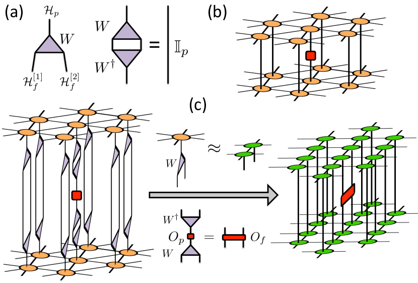
Figure 1: (Color online) (a) Isometry $W$ projects the fine-grained Hilbert spaces $\mathcal{H}^{[1]}_{f}$ and $\mathcal{H}^{[2]}_{f}$ into the physical space $\mathcal{H}_{p}$. The isometry verifies $W^{\dagger}W={\mathbb{I}_{p}}$, with ${\mathbb{I}_{p}}$ the identity in the physical space; (b) Expectation value of an one-site operator for a 2d PEPS on a triangular lattice; (c) By introducing resolutions of the identity $W^{\dagger}W$ at every site, we can rewrite the expectation value in terms of a fine-grained two-site operator and fine-grained PEPS tensors on a 2d square lattice.

The idea above is generalized as follows: a physical degree of freedom described by a Hilbert space $\mathcal{H}_{p}$ can be understood as the coarse-grained space of some other fine-grained Hilbert spaces $\mathcal{H}_{f}^{[1]}$ and $\mathcal{H}_{f}^{[2]}$ via some isometry $W$, i.e.,

$$W:\mathcal{H}_{f}^{[1]}\otimes\mathcal{H}_{f}^{[2]}\longrightarrow\mathcal{H}_{p},$$ (1)

with $W=\sum_{if_{1}f_{2}}W^{i}_{f_{1}f_{2}}|f_{1}\rangle|f_{2}\rangle\langle i|$. In TN language, the 3-index tensor $W^{i}_{f_{1}f_{2}}$ coarse-grains the indices $f_{1}$ and $f_{2}$ into $i$. Seen in reverse, the physical index $i$ is fine-grained into indices $f_{1}$ and $f_{2}$ by the isometric tensor $W^{i}_{f_{1}f_{2}}$. Since $W$ is an isometry, it implies that $W^{\dagger}W={\mathbb{I}_{p}}$, with ${\mathbb{I}_{p}}$ the identity in the physical Hilbert space $\mathcal{H}_{p}$, see Fig. 1.a. Let us remark that we considered here the case of two fine-grained Hilbert spaces, but the idea can be easily generalized to having more than two. In fact, the whole isometry $W$ could even have a TN structure itself (as in, e.g., the multiscale entanglement renormalization ansatz (MERA) Vidal (2007)), if required. Generically, the isometry can also be understood in the language of entanglement branching operators Harada (2018).

Next, we apply this fine-graining to the physical degrees of freedom of many-body systems with high-connectivity, which allows us to simplify the underlying lattice structure and therefore make them more amenable to TN simulation methods. Let us consider, without loss of generality, the case of a triangular lattice. As shown in Fig. 1.b-c, fine-graining every site maps the triangular lattice into a square lattice. The key point is to realize that, in such a scenario, operators on the triangular lattice are mapped to operators on the fine-grained square lattice via the isometry W, as shown in Fig.1.c. For instance, for an one-site operator $O_{p}$ acting on one site of the physical lattice, one has

$$O_{f}=WO_{p}W^{\dagger}$$ (2)

with $O_{f}$ the corresponding operator on the fine-grained lattice. In the case of the triangular lattice that we are discussing, this maps a one-site operator $O_{p}$ on the triangular lattice to a two-site operator $O_{f}$ on the square lattice. In general, for a fine-graining isometry involving $n$ fine-grained Hilbert spaces, an $m$-body operator on the original lattice is mapped to an $(n\times m)$-body operator in the fine-grained one.

Our method can thus be summarized in three steps:

1. Find an isometry $W$ that reduces the connectivity of the lattice after fine-graining.

2. Use $W$ to map all operators involved in the TN algorithm to their fine-grained versions.

3. Run the TN algorithm on the fine-grained lattice using the fine-grained operators.

The mapping between lattices preserves locality inasmuch the isometry $W$ is local. This implies, for instance, that local expectation values in the original lattice may also be mostly local in the fine-grained one. Notice also that, at the level of TN optimization and calculation of local expectation values, one can fully operate in the fine-grained space only, see Fig. 1.c for an example.

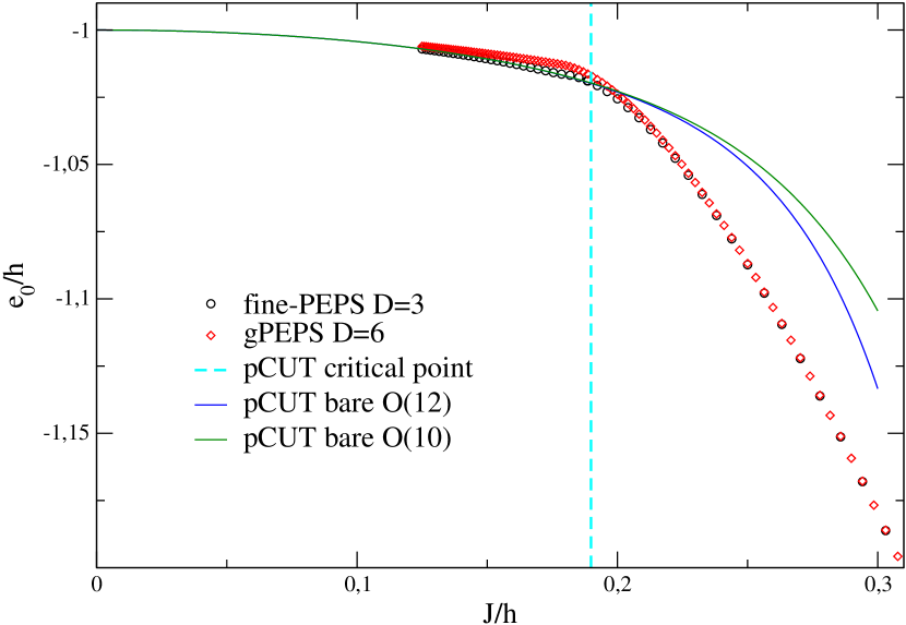
Figure 2: (Color online) Ground-state energy per site for the ferromagnetic spin-$1$ quantum Ising model on the triangular lattice, as computed by fine-PEPS (circles), gPEPS (diamonds), and pCUTs (solid lines). The vertical dashed line refers to the critical point $(h/J)_{\rm c}^{\rm pCUT}=0.1898(1)$ from extrapolating the one-particle pCUT gap.

A number of practical considerations are in order. First, the isometry $W$ is a new degree of freedom that enters the TN algorithm. It could be optimized following a MERA-like procedure, yet another option is to fix it to some reasonable choice and optimize over the tensors of the fine-grained TN. This choice is not unique and moreover it is also reasonable to think that some isometries may work better than others in practice depending on the symmetries of the system. Generally, an isometry that splits the physical Hilbert space symmetrically seems to be beneficial (e.g., a decomposition of $1=0\otimes 1$ is valid but unbalanced). Second, interaction terms in the fine-grained Hamiltonian may become of slightly longer range. For instance, for a Hamiltonian with nearest-neighbour interactions on the triangular lattice, one gets interactions that span over four sites in the fine-grained square lattice. Third, and as we said above, more complicated isometries are also possible, even with an internal TN structure. Further discussion about the details of the method and the relevant tensor updates can be found in Ref. Philipp Schmoll, Saeed S. Jahromi, Max Hormann, Matthias Muhlhauser, Kai Phillip Schmidt and Orus ; Vidal (2003).

Numerical results.- In order to benchmark the validity of our approach we computed the ground-state properties of several models on the triangular lattice for a unit cell of $2\times 2$ tensors. For this, we used fine-graining together with the infinite-PEPS algorithm Phien et al. (2015); Orús and Vidal (2009) on the square lattice with a $2\times 4$ unit cell and simple update, also for four-body interactions, and computed expectation values with Corner Transfer Matrix (CTM) techniques Orús and Vidal (2009); Corboz et al. (2014, 2010a).

The first model that we considered is the spin-$1$ ferromagnetic quantum Ising model in a transverse field, described by the Hamiltonian Powalski et al. (2013)

$$H=-J\sum_{\langle i,j\rangle}\sigma^{[i]}_{x}\sigma^{[j]}_{x}-h\sum_{i}\sigma^{[i]}_{z},$$ (3)

with $\sigma^{[i]}_{\alpha}$ the $3\times 3$ spin-one matrix at site $i$, $J>0$ the ferromagnetic interaction strength, and $h$ the magnetic field. It realizes a polarized phase for small $J/h$ and a symmetry-broken ordered phase for large $J/h$ separated by a second-order phase transition in the 3d Ising universality class. The location of the critical point can be estimated precisely by the pCUT series of the one-particle gap in the polarized phase using Dlog Padé extrapolation Guttmann (1989) which yields $(J/h)_{\rm c}^{\rm pCUT}=0.1898(1)$ or equivalently in the inverse unit $(h/J)_{\rm c}^{\rm pCUT}=5.269(3)$ Philipp Schmoll, Saeed S. Jahromi, Max Hormann, Matthias Muhlhauser, Kai Phillip Schmidt and Orus ; Kos et al. (2016).

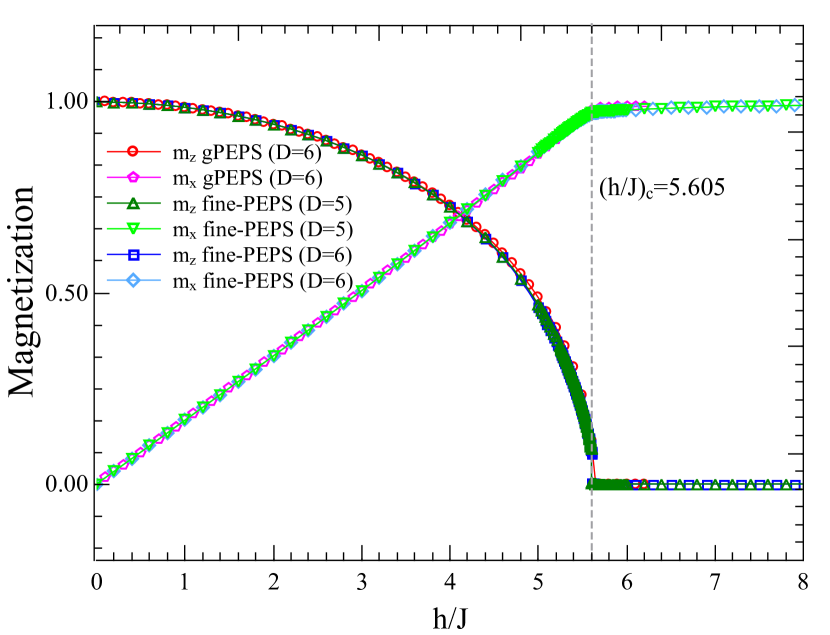
Figure 3: (Color online) Longitudinal and transverse magnetization per site for the ferromagnetic spin-$1$ quantum Ising model on the triangular lattice, as computed by fine-PEPS and gPEPS.

For the fine-PEPS we choose to fine-grain each spin-$1$ into two spins-$1/2$ via an isometry that equals a Clebsch-Gordan coefficient, $W_{m_{1},m_{2}}^{m}=\langle 1/2,1/2,m_{1},m_{2}|1/2,1/2,1,m\rangle$. In Fig. 2 we show the ground-state energy per site computed by fine-graining (fine-PEPS) with PEPS bond dimension $D=3$, as well as using gPEPS with $D=6$ and pCUT up to $O(12)$ in the high-field expansion in $J/h$. Remarkably, even for a small bond dimension $D=3$, the agreement of fine-PEPS with pCUT for $J/h\leq(J/h)_{\rm c}^{\rm pCUT}$ within the polarized phase and with gPEPS for large $J/h$ inside the symmetry-broken ordered phase is almost perfect. In Fig. 3 we also plot longitudinal and transverse magnetizations as computed by fine-PEPS and gPEPS, also in excellent agreement, and with an approximate quantum critical point of $(h/J)_{\rm c}^{\rm fine-PEPS}\approx 5.605$. Notice that the critical point obtained by the two tensor network methods deviates from the pCUT result $(J/h)_{\rm c}^{\rm pCUT}$. This is, however, due to the simple update, which does not make use of the full environment when updating the tensors. Simulations with the full environment would improve the accuracy close to criticality, shall this be required.

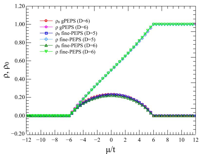
Figure 4: (Color online) Particle density and condensate fraction for the hard-core Bose-Hubbard model on the triangular lattice, for $t=1$, as computed by fine-PEPS and gPEPS.

Furthermore, we simulated the Bose-Hubbard model on the triangular lattice, described by the Hamiltonian Kshetrimayum et al. (2019); Wang et al. (2013)

$$H=-t\sum_{\langle i,j\rangle}\left(a^{\dagger}_{i}a_{j}+h.c.\right)+\frac{U}{2}\sum_{i}n_{i}\left(n_{i}-1\right)-\mu\sum_{i}n_{i},$$ (4)

with $a_{j},a_{j}^{\dagger}$ and $n_{j}=a_{j}^{\dagger}a_{j}$ respectively being bosonic annihilation, creation and number operators at site $j$, $t$ the hopping strength, $U$ the on-site density-density interaction, and $\mu$ the chemical potential.

In the hard-core limit $U\rightarrow\infty$, where individual sites are either empty or occupied by one boson, this model realizes two exact gapped Mott phases with density zero and one as well as an intermediate gapless superfluid phase. The phase transitions at $(\mu/J)_{\rm c}=\pm 6$ between the Mott and superfluid phases can be determined exactly by first-order perturbation theory for the one-particle gap of the two Mott phases Philipp Schmoll, Saeed S. Jahromi, Max Hormann, Matthias Muhlhauser, Kai Phillip Schmidt and Orus . Technically, we fine-grain every hard-core boson into two hard-core bosons via an isometry with non-zero coefficients $W_{0,0}^{0}=1,W_{1,0}^{1}=W_{0,1}^{1}=1/\sqrt{2}$. Thus, if the physical site is occupied, then the hard-core boson can be on either of the fine-grained sites. In Fig. 4 we show our numerical results for the particle density $\rho=\langle a^{\dagger}_{j}a_{j}\rangle$ and the condensate fraction $\rho_{0}=|\langle a_{j}\rangle|^{2}$ for fine-PEPS and gPEPS both up to $D=6$ and with $t=1$, showing excellent agreement in the superfluid and Mott-insulator phases.

Furthermore, we considered the soft-core case up to two bosons per lattice site so that the ground-state phase diagram consists of three Mott lobes with densities $n\in\{0,1,2\}$ and superfluid phases. The empty ($n=0$) and completely filled ($n=2$) Mott states are again exact eigenstates of the system and the corresponding one-particle gap $\Delta_{n=0}^{\rm p}=-\mu-6t$ (one-hole gap $\Delta_{n=2}^{\rm h}=-U+\mu-12t$) can be calculated exactly Philipp Schmoll, Saeed S. Jahromi, Max Hormann, Matthias Muhlhauser, Kai Phillip Schmidt and Orus . This is different for the Mott phase with $n=1$ where the hopping term introduces quantum fluctuations. For the fine-PEPS we break down again each local site in terms of two hard-core bosons which, when both occupied, result in a double occupied physical site. For this we use an isometry with non-zero coefficients $W_{0,0}^{0}=1,W_{1,0}^{1}=W_{0,1}^{1}=1/\sqrt{2},W_{1,1}^{2}=1$. The particle density and condensate fraction for soft-core bosons is shown in Fig. 5, computed by fine-PEPS up to $D=5$ and gPEPS up to $D=6$ with $t=0.01$ and $U=1$, again showing an excellent agreement in all superfluid and Mott-insulating phases.

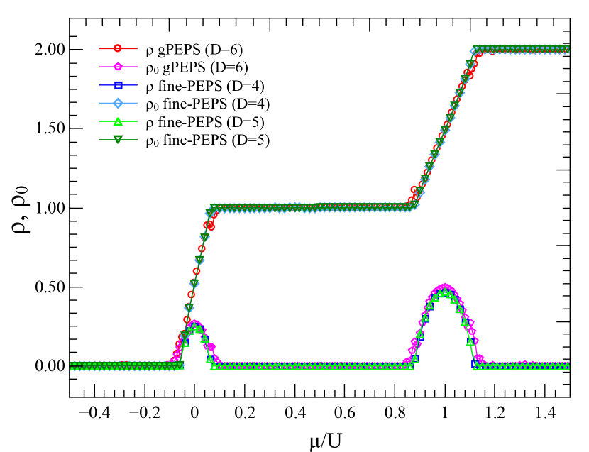
Figure 5: (Color online) Particle density and condensate fraction for the soft-core Bose-Hubbard model on the triangular lattice with up to $2$ bosons per site, for $t=0.01$ and $U=1$, as computed by fine-PEPS and gPEPS.

In order to show the potential of our method in higher dimensions we consider Eq. 3 on a 3d stacked triangular lattice (see Philipp Schmoll, Saeed S. Jahromi, Max Hormann, Matthias Muhlhauser, Kai Phillip Schmidt and Orus for a depiction of the lattice structure). The location of the critical point with expected mean-field exponents can be estimated again precisely by extrapolating the pCUT series of the one-particle gap in the polarized phase which yields $(h/J)_{\rm c}^{\rm pCUT}=7.45(1)$ Philipp Schmoll, Saeed S. Jahromi, Max Hormann, Matthias Muhlhauser, Kai Phillip Schmidt and Orus . Here the local iPEPS tensors have eight virtual indices besides the physical one. Using the same idea of fine-graining the local Hilbert space of the spin-ones, the model is mapped onto a cubic lattice. Importantly, this mapping enables the use of 3d CTM schemes to perform the contraction of the infinite 3d lattice. Due to the reduced importance of quantum fluctuations in 3d we choose however to use the mean-field environment for every local iPEPS tensor in the present simulations. Fig. 6 shows the magnetization as well as the ground-state energy as a function of the magnetic field. We find $(h/J)_{\rm c}^{\rm fine-PEPS}\approx 7.59$ which is in good agreement with that of gPEPS and pCUT.

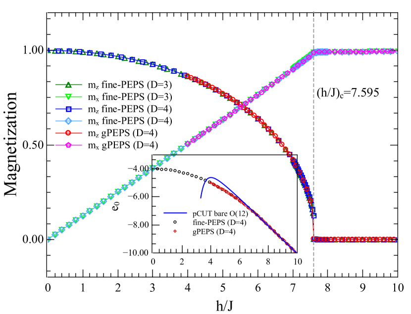
Figure 6: (Color online) Longitudinal and transverse magnetization per site for the ferromagnetic spin-$1$ quantum Ising model on the 3d stacked-triangular lattice, as computed by fine-PEPS and gPEPS. The inset shows the ground-state energy per site of the ITF model obtained with fine-PEPS, gPEPS, and pCUT (bare order 12 is shown).

Conclusions.- In this paper we have proposed an efficient approach to deal with lattices of high connectivity in TN methods, by using a fine-graining of the physical degrees of freedom. Under suitable conditions, this fine-graining simplifies the lattice and essentially keeps locality of interactions. After a fine-graining of operators, the approach allows us to apply usual TN methods on simpler lattices in a remarkably efficient way. Most importantly, the fine-graining allows us to use the CTM method for approximating the contraction of the infinite TN, in turn, capturing all quantum correlations into the environment of local tensors which are also essential for the full update iPEPS simulations. This is a huge advancement over other TN methods such as gPEPS which use mean-field environments for calculations of the expectation value of local operators and correlators. We have explained in detail the example of the 2d triangular lattice, which in our approach can be simulated using standard 2d square-lattice PEPS algorithms. Our method has been benchmarked with numerical simulations of the ground state of paradigmatic magnetic and bosonic models in 2d and 3d, with excellent accuracy when compared to other methods such as pCUT and gPEPS. We believe that the approach in this paper will allow to overcome the computational cost associated to simulating lattices of high connectivity, such as the ones typically found for higher dimensional systems and frustrated quantum antiferromagnets and will become an instrumental tool in the discovery of new exotic phases of quantum matter.