Universal trapping law induced by atomic cloud in single-photon cooperative dynamics

Abstract

Single-photon cooperative dynamics of an assembly of two-level quantum emitters coupled by a bosonic bath are investigated. The bosonic bath is general and it can be anything as long as the exchange of excitations between quantum emitters and bath is present. In these systems, it is found that the population on the excited emitter keeps a simple and universal trapping law due to the existence of system’s dark states. Different from the trapping regime caused by photon-emitter dressed states, this type of trapping is only associated with the number of quantum emitters. According to the trapping law, the cooperative spontaneous emission at single-photon level in this kind of systems is universally inhibited when the emitter number is large enough.

Cooperative light-matter interaction plays an important role in quantum electrodynamics Dicke54 ; Mandel95 and is useful for various applications of quantum optics such as optical quantum-state storage Eisaman04 ; Kalachev06 ; Kalachev07 , quantum communication Kuzmich03 ; Eisaman05 , and quantum information processing Porras08 . For a single excitation of an ensemble of quantum emitters, the rate and the direction of the cooperative spontaneous emission can be strongly modified by different light-field environments. While the size and the shape of the ensemble have been investigated Scully06 ; Li06 ; Miroshnychenko13 , an ensemble of atoms with a single collective excitation also exhibits a dynamics characterized by revivals for different atom numbers in a bosonic bath with linear dispersion relation Kumlin18 .

However, until now, almost all the results and conclusions about the single-photon cooperative dynamics provided by the published papers are based on the specific light-field environments and the specific coupling coefficient between quantum emitters and photon Cummings83 ; FWC85 ; Benivegna88 ; Buzek89 ; Buzek99 ; AAS08 ; SD08 ; Scully09 ; AAS10 ; SZ12 ; Li12 ; Boag13 ; Xu13 ; Feng14 ; Liao15 ; Jenkins17 . If the light-field environments and coupling coefficient are changed, will these results and conclusions change or keep the same?

Here, we focus on the single-photon cooperative dynamics in a system that the light-field environment and the coupling coefficient are general and physical. The emitters are assumed to be placed much closer than the wavelength of radiation field and thus the emitters are efficiently coupled by the radiation field without retardation effects.

In this paper, we report that there is a universal trapping law in the single-photon cooperative dynamics based on an analytical analysis which is beyond Wigner-Weisskopf approximation and Markovian approximation. A direct conclusion comes from this law is that the spontaneous emission dynamics in this system is suppressed if the number of the emitters is large enough.

We begin with the system that contains $M$ two-level atoms coupled to the radiation field in an environment with a general dispersion relation $\omega_{k}$. The atoms are characterized by ground state $\left|g\right\rangle$ and excited state $\left|e\right\rangle$. The Hamiltonian of this system in the rotating-wave approximation takes the form (with $\hbar=1$)

$$H =\sum_{k}\omega_{k}a_{k}^{{\dagger}}a_{k}+\sum_{j=1}^{M}\Omega_{j}\left|e_{j}\right\rangle\left\langle e_{j}\right|$$

$$+\sum_{j,k}V_{k,j}\left(\sigma_{j}^{+}a_{k}+\sigma_{j}^{-}a_{k}^{{\dagger}}\right)$$ (1)

where the first term describes the light field and $a_{k}^{{\dagger}}$ ($a_{k}$) denotes the creation (annihilation) operator of photon with momentum $k$. The second term represents two-level atoms and $\Omega_{j}$ is atom’s transition frequency. Here, we set the ground energy of atoms to be zero as reference. The last term represents the interaction between photon and atoms. $\sigma_{j}^{+}=\left|e_{j}\right\rangle\left\langle g_{j}\right|$ ($\sigma_{j}^{-}=\left|g_{j}\right\rangle\left\langle e_{j}\right|$) is the raising (lowering) operator acting onto the $j$th atom and $V_{k,j}$ is the coupling strength.

To investigate the dynamics of atoms when one of them is excited, we start from the time-dependent Schrödinger equation

$$i\frac{\partial}{\partial t}\left|\psi\left(t\right)\right\rangle=H\left|\psi\left(t\right)\right\rangle$$ (2)

where $|\psi\left(t\right)\rangle$ is the state of the system at time $t$. Since the total excitation number $N=\sum_{k}\omega_{k}a_{k}^{{\dagger}}a_{k}+\sum_{j=1}^{M}|e_{j}\rangle\langle e_{j}|$ is conserved, the state $|\psi\left(t\right)\rangle$ with $N=1$ can be expanded as $|\psi(t)\rangle=\sum_{j}A_{j}(t)|g_{1}g_{2}...e_{j}...g_{M},0\rangle+\sum_{k}C_{k}(t)|g_{1}g_{2}...g_{M},1_{k}\rangle$, where $A_{j}(t)$ is the probability amplitude of the state with $j$th atom in the excited state and the others in the ground states and no photon in the environment, while $C_{k}(t)$ represents the probability amplitude for finding all atoms to be in the ground states and one photon in the environment. Take $|\psi(t)\rangle$ into Eq. (2), one obtains the equations for $A_{j}(t)$ and $C_{k}(t)$

$$i\frac{\partial A_{j}\left(t\right)}{\partial t}=\Omega_{j}A_{j}\left(t\right)+\sum_{k}V_{k,j}C_{k}\left(t\right)\text{,}$$ (3)

$$i\frac{\partial C_{k}\left(t\right)}{\partial t}=\omega_{k}C_{k}\left(t\right)+\sum_{j}V_{k,j}A_{j}\left(t\right)\text{.}$$ (4)

The method based on Wigner-Weisskopf approximation or Markovian approximation theory is widely used to solve the dynamical equations in Eq. (3) and (4) with specific $\omega_{k}$ and $V_{k,j}$, which leads to a result that the excited atomic population reveals exponential decay or the population decay is complete. However, it has been pointed out that an important information about the population trapping will be lost when one of this two kinds of approximation theories is used John94 ; Tudela17 ; Tudela172 .

To go beyond Wigner-Weisskopf approximation and Markovian approximation, we take a Laplace transform of Eq. (3) and (4) and it gives

$$i\left[-A_{j}\left(0\right)+s\tilde{A}_{j}\left(s\right)\right]=\Omega_{j}\tilde{A}_{j}\left(s\right)+\sum_{k}V_{k,j}\tilde{C}_{k}\left(s\right)\text{,}$$ (5)

$$i\left[C_{k}\left(0\right)+s\tilde{C}_{k}\left(s\right)\right]=\omega_{k}\tilde{C}_{k}\left(s\right)+\sum_{j}V_{k,j}\tilde{A}_{j}\left(s\right)\text{.}$$ (6)

Denote the initial excited atom as $j_{0}$, i.e., the initial amplitudes are $A_{j_{0}}\left(0\right)=1$, $A_{j}\left(0\right)=0$ ($j\neq j_{0}$) and $C_{k}\left(0\right)=0$, the expression of $\tilde{A}_{j_{0}}\left(s\right)$ can be acquired

$$\tilde{A}_{j_{0}}\left(s\right)=i\frac{is-\Omega-(M-1)f\left(s\right)}{\left(is-\Omega\right)\left[is-\Omega-Mf\left(s\right)\right]}$$ (7)

where $f\left(s\right)\equiv\sum_{k}V_{k}^{2}/(is-\omega_{k})$. Here it has been assumed that the atoms are identical and thus $\Omega_{1}=\Omega_{2}=...=\Omega_{M}=\Omega$, $V_{k,1}=V_{k,2}=...=V_{k,M}=V_{k}$. The amplitude $A_{j_{0}}\left(t\right)$ is given by the inverse Laplace transform $A_{j_{0}}\left(t\right)=\frac{1}{2\pi i}\int_{\sigma-i\infty}^{\sigma+i\infty}\tilde{A}_{j_{0}}\left(s\right)e^{st}ds$, which leads to

$$A_{j_{0}}\left(t\right) =\sum_{n}\frac{s+i\Omega+i(M-1)f\left(s\right)}{[F\left(s\right)]^{\prime}}e^{st}|_{s=x_{n}^{\left(1\right)}}$$

$$-\int_{C}\frac{s+i\Omega+i(M-1)f\left(s\right)}{2\pi iF\left(s\right)}e^{st}ds$$ (8)

where $F\left(s\right)\equiv(s+i\Omega)[s+i\Omega+iMf\left(s\right)]$ and $[F\left(s\right)]^{\prime}$ means the derivative of $F\left(s\right)$ with respect to $s$. $x_{n}^{\left(1\right)}$ is the roots of the equation $F\left(s\right)=0$ in the complex plane except the regions in order to ensure that the integrand is single-valued function. $C$ is the integration contour based on residue theorem. Generally, $C$ is associated with the specific expression of $V_{k}$ and $\omega_{k}$. Different $V_{k}$ and $\omega_{k}$ lead to different integration contour $C$. However, a common conclusion that does not depend on specific $V_{k}$ and $\omega_{k}$ is that the second term of $A_{j_{0}}\left(t\right)$ in Eq. (8) goes to zero when time $t$ tends to infinity due to the factor $e^{st}$ Riley06 .

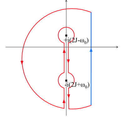
Figure 1: Integration contours for the calculation of $A_{j_{0}}(t)$ in the coupled-cavity system. The red line is the integration contour $C$.

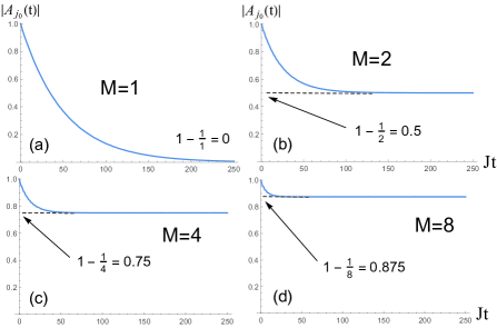
Figure 2: Time evolution of the population $|A_{j_{0}}\left(t\right)|$ on the excited atom with different atom number in the coupled-cavity system. The coupling strength $g_{0}=0.2J$. The detuning $\delta_{1}\equiv\Omega-\omega_{0}=0$.

The physics in Eq. (8) is not obvious. We transform Eq. (8) into another form which is the key point for the analysis in the following

$$A_{j_{0}}\left(t\right) =\frac{M-1}{M}e^{-i\Omega t}+\sum_{m}\frac{e^{st}}{M\left[G\left(s\right)\right]^{\prime}}|_{s=x_{m}^{\left(2\right)}}$$

$$-\int_{C}\frac{G(s)-if\left(s\right)}{2\pi iF\left(s\right)}e^{st}ds$$ (9)

where $G(s)\equiv s+i\Omega+iMf\left(s\right)$ and $x_{m}^{\left(2\right)}$ is the roots of the equation $G(s)=0$. Here, the equation $G(-iE)=0$ is nothing but the system’s eigenenergy equation of photon–atom dressed state. In fact, the second term of $A_{j_{0}}\left(t\right)$ in Eq. (9) comes from system’s photon-atom bound states that the populations of field modes are not zero and the third term comes from system’s scattering states John94 ; Qiao19 . The first term in Eq. (9) is only related with the atom’s transition frequency and the number of atoms. It comes from system’s dark state with energy $\Omega$ that all the excitation number focuses on the atoms and the populations of field modes are zero Sun03 ; S2un03 . This kind of dark state is universal in this kind of system. It is caused by the collective coherence of atomic clouds. So the trapping associated with the dark state is universal no matter whether the role of the second term in Eq. (9) is important or not.

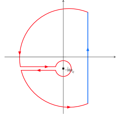
Figure 3: Integration contours for the calculation of $A_{j_{0}}(t)$ in the photonic crystal system. The red line is the integration contour $C$.

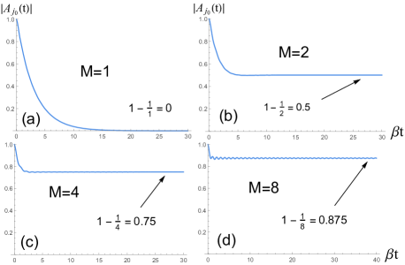
Figure 4: Time evolution of the population $|A_{j_{0}}\left(t\right)|$ on the excited atom with different atom number in the photonic crystal system. The detuning $\delta_{2}\equiv\Omega-\omega_{c}=6.5\beta$. Here $\beta^{3/2}\equiv(\Omega^{2}d^{2})/(6\pi\epsilon_{0}B^{3/2})$.

When the equation $G(s)=0$ has no roots or that the system’s parameters satisfy the condition $|1/\{M[G(x_{m}^{(2)})]^{\prime}\}|<<1$, the final result of the amplitude $A_{j_{0}}\left(t\right)$ at $t=\infty$ is

$$\left|A_{j_{0}}\left(\infty\right)\right|=1-\frac{1}{M}$$ (10)

which is only related with the atom number. This trapping phenomenon takes place when the number $M>1$.

To check this universal trapping, we now present two examples. One is the system of one-dimensional coupled-cavity waveguide, in which the dispersion $\omega_{k}=\omega_{0}-2J\cos(k)$ and the coupling coefficient $V_{k}=g_{0}$ Zhou08 ; Longo10 ; Zhou13 . Here $\omega_{0}$ is the on-site energy of each cavity and $J$ represents the hopping energy of the photon between two neighbouring cavity. The other is the system of three-dimensional photonic crystal with $\omega_{\mathbf{k}}=\omega_{c}+B(\mathbf{k}-\mathbf{k}_{0})^{2}$ and $V_{\mathbf{k}}=\Omega d\sqrt{\frac{1}{2\epsilon_{0}\omega_{\mathbf{k}}V}}\mathbf{e}_{k}\cdot\mathbf{u}$ John90 ; John94 ; Zhu97 ; Lambropoulos00 . $d$ and $\mathbf{u}$ are the magnitude and unit vector of atomic dipole moment. $V$ is the volume and $\mathbf{e}_{k}$ is the two transverse unit vectors of polarization. Both of the two systems have been extensively studied theoretically and experimentally in recent years. For the coupled-cavity system, the integration contour $C$ is shown by the red line in Fig. 1. When $\Omega=\omega_{0}$, the condition $|1/\{M[G(x_{m}^{(2)})]^{\prime}\}|<<1$ can be easily satisfied. In Fig. 2, we plot the time evolution of $A_{j_{0}}\left(t\right)$ for different number of atoms. One see that $|A_{j_{0}}(\infty)|$ meets the value $1-1/M$. For the photonic crystal system, the integration contour $C$ is plotted with the red line in Fig. 3. The time evolution of $A_{j_{0}}\left(t\right)$ is shown in Fig. 4. The trapping law $1-1/M$ is also obeyed when the condition $|1/\{M[G(x_{m}^{(2)})]^{\prime}\}|\ll 1$ is satisfied.

To sum up, we have explored the single-photon cooperative dynamics in an ensemble of two-level atoms which is couple to a general bosonic bath. The size of the ensemble is much smaller than the wavelength of radiation field. The bosonic bath can be photonic crystal, waveguide, or anything else as long as the exchange of excitations between atoms and bath can take place. It is found that there is a universal trapping caused by system’s dark state. This kind of trapping obeys a simple law that is only related with the number of atoms. A direct conclusion comes from this law is that the single-photon cooperative spontaneous emission is suppressed when there are many enough atoms. Besides, due to the presence of this trapping, the energy of the radiation field will be less than the initial total energy $E_{tot}=\Omega$.

I Acknowledgements

This work is supported by the National Basic Research Program of China (Grant No. 2016YFA0301201 & No. 2014CB921403), the NSFC (Grant No. 11534002), and the NSAF (Grant No. U1730449 & No. U1530401).

References

- (1) R. H. Dicke, Phys. Rev. 93, 99 (1954).
- (2) L. Mandel and E. Wolf, Optical Coherence and Quantum Optics (Cambridge University Press, Cambridge, UK, 1995).
- (3) M. D. Eisaman, L. Childress, A. André, F. Massou, A. S. Zibrov, and M. D. Lukin, Phys. Rev. Lett. 93, 233602 (2004).
- (4) A. Kalachev and S. Kröll, Phys. Rev. A 74, 023814 (2006).
- (5) A. Kalachev, Phys. Rev. A 76, 043812 (2007).
- (6) A. Kuzmich, W. P. Bowen, A. D. Boozer, A. Boca, C. W. Chou, L.-M. Duan, and H. J. Kimble, Nature (London) 423, 731 (2003).
- (7) M. D. Eisaman, A. André, F. Massou, M. Fleischhauer, A. S. Zibrov, and M. D. Lukin, Nature (London) 438, 837 (2005).
- (8) D. Porras and J. I. Cirac, Phys. Rev. A 78, 053816 (2008).
- (9) M. O. Scully, E. S. Fry, C. H. R. Ooi, and K. Wódkiewicz, Phys. Rev. Lett. 96, 010501 (2006).
- (10) Y. Li, Z. D. Wang, and C. P. Sun, Phys. Rev. A 74, 023815 (2006).
- (11) Y. Miroshnychenko, U. V. Poulsen, and K. Molmer, Phys. Rev. A 87, 023821 (2013).
- (12) J. Kumlin, S. Hofferberth, and H. P. Büchler, Phys. Rev. Lett. 121, 013601 (2018).
- (13) F. W. Cummings and A. Dorri, Phys. Rev. A 28, 2282 (1983).
- (14) F. W. Cummings, Phys. Rev. Lett. 54, 2329 (1985); Phys. Rev. A 33, 1683 (1986).
- (15) G. Benivegna and A. Messina, Phys. Lett. A 126, 249 (1988).
- (16) V. Buzek, Phys. Rev. A 39, 2232 (1989).
- (17) V. Buzek, G. Drobny, M. G. Kim, M. Havukainen, and P. L. Knight, Phys. Rev. A 60, 582 (1999).
- (18) A. A. Svidzinsky, J. T. Chang, and M. O. Scully, Phys. Rev. Lett. 100, 160504 (2008).
- (19) S. Das, G. S. Agarwal, and M. O. Scully, Phys. Rev. Lett. 101, 153601 (2008).
- (20) M. O. Scully and A. A. Svidzinsky, Science 325, 1510 (2009).
- (21) A. A. Svidzinsky, J.-T. Chang, and M. O. Scully, Phys. Rev. A 81, 053821 (2010).
- (22) S. Zhang, C. Liu, S. Zhou, C.-S. Chuu, M. M. T. Loy, and S. Du, Phys. Rev. Lett. 109, 263601 (2012).
- (23) Y. Li, J. Evers, H. Zheng, and S.-Y. Zhu, Phys. Rev. A 85, 053830 (2012).
- (24) G. Y. Slepyan and A. Boag, Phys. Rev. Lett. 111, 023602 (2013).
- (25) D. Z. Xu, Y. Li, C. P. Sun, and P. Zhang, Phys. Rev. A 88, 013832 (2013).
- (26) W. Feng, Y. Li, and S.-Y. Zhu, Phys. Rev. A 89, 013816 (2014).
- (27) Z. Liao, X. Zeng, S.-Y. Zhu, and M. S. Zubairy, Phys. Rev. A 92, 023806 (2015).
- (28) S. D. Jenkins, J. Ruostekoski, N. Papasimakis, S. Savo, and N. I. Zheludev, Phys. Rev. Lett. 119, 053901 (2017).
- (29) S. John and T. Quang, Phys. Rev. A 50, 1764 (1994).
- (30) A. González-Tudela and J. I. Cirac, Phys. Rev. Lett. 119, 143602 (2017).
- (31) A. González-Tudela and J. I. Cirac, Phys. Rev. A 96, 043811 (2017).
- (32) K. F. Riley, M. P. Hobson, and S. J. Bence, Mathematical Methods for Physics and Engineering, 3rd ed. (Cambridge University Press, Cambridge, England, 2006).
- (33) L. Qiao, Y. J. Song, and C. P. Sun, Phys. Rev. A 100, 013825 (2019).
- (34) C. P. Sun, Y. Li, and X. F. Liu, Phys. Rev. Lett. 91, 147903 (2003).
- (35) C. P. Sun, S. Yi, and L. You, Phys. Rev. A 67, 063815 (2003).
- (36) L. Zhou, Z. R. Gong, Y. X. Liu, C. P. Sun, and F. Nori, Phys. Rev. Lett. 101, 100501 (2008).
- (37) P. Longo, P. Schmitteckert, and K. Busch, Phys. Rev. Lett. 104, 023602 (2010).
- (38) L. Zhou, L. P. Yang, Y. Li, and C. P. Sun, Phys. Rev. Lett. 111, 103604 (2013).
- (39) S. John and J. Wang, Phys. Rev. Lett. 64, 2418 (1990).
- (40) S.-Y. Zhu, H. Chen, and H. Huang, Phys. Rev. Lett. 79, 205 (1997).
- (41) P. Lambropoulos, G. M. Nikolopoulos, T. R. Nielsen, and S. Bay, Rep. Prog. Phys. 63, 455 (2000).