Exact Amplitude Distributions of Sums of Stochastic Sinusoidals and their Application in Bit Error Rate Analysis

Abstract

We consider a model applicable in many communication systems where the sum of $n$ stochastic sinusoidal signals of the same frequency, but with random amplitudes as well as phase angles is present. The exact probability distribution of the resulting signal’s amplitude is of particular interest in many important applications, however the general problem has remained open. We derive new general formulae for the resultant amplitude’s distribution, in terms of any given general joint density of the random variables involved. New exact probability densities of cases of interest follow from the general formulae which are applied to the problem of the exact evaluation of the bit error rate performance in narrowband multipath fading channels that consist of a small number of jointly dependent resolvable multipath components. The numerical results are compared with those of the currently popular method of Gaussian approximation. These are consistent with simulations, and show significant increase in accuracy particularly for small number of components.

I Introduction

In many communication systems the received signal can be expressed as [1]-[4]

$$r(t)=\sum_{i=1}^{n}A_{i}\cos(\omega t+\phi_{i})+Z(t)\ .$$ (1)

The first term in (1) represents the desired signal component with amplitude $A_{1}$, frequency $\omega$, and phase $\phi_{1}$, mixed with interference that is produced either unintentionally by a multiple access process, reflections of the desired signal, or intentionally by a certain jammer. The second term, $Z(t)$, is an additive white Gaussian noise (AWGN) with two-sided power spectral density of $N_{0}/2$.

In general the amplitudes $(A_{1},A_{2},...,A_{n})$, and the phases $(\phi_{1},\phi_{2},...,\phi_{n})$, may all be random variables, with a given joint probability distribution function, which is the framework treated in this paper. In specific applications however, the statistical properties of these variables, and the value of $n$, depend on the particular channel model and the application considered. For example, in the case of narrowband local area UHF and microwave propagation, the amplitudes are considered to be constants and the phases are independent and uniformly distributed over $[-\pi,\pi]$ [1]-[3]. The number of multipath components $n$ is determined based on the terrain of the surroundings at the receiver side. Similar assumptions are usually made for synchronous frequency hopping spread spectrum systems (FH-SSS) with multiple access interference (MAI) or multitone jamming (MTJ) with AWGN [4]-[18]. The value of $n$ in multiple access systems corresponds to the number of simultaneous users and it is modelled as a random variable with binomial distribution.

The case where the amplitudes are random has also a wide range of applications. For example, Beaulieu et al [7] have modelled the amplitudes as a Nakagami-$m$ random variables to analyze the performance of wireless networks with cochannel interference. The Rayeligh-distributed amplitudes model was adapted for FH-SSS with orthogonal frequency division multiplexing (OFDM) in [18], [8].

In evaluation of the performance of communication systems with received signals such as $r(t)$ in (1), the knowledge of the pdf (probability density function) of the resultant amplitude or envelope is of crucial importance. Rice [9] stated that the cdf (cumulative distribution function) of the envelope of some special cases of (1) may be represented by a Fourier-Bessel Transform. Kluyver [10] considered the case of $n$ randomly phased sine waves in the absence of noise and gave a corresponding equation for the special case in [9]. Simon [11] considered a special recursive case of (1) without noise, where all the amplitudes are fixed, and each new phase angle is assumed to be equal to the resultant of all the previous ones, plus an independent uniformly distributed angle. Thus, he deduced a recursive formula for the pdf of the squared envelope in this special case (see also Section III below). Helstrom [12] derived the amplitude pdf of the sum of two sinusoidals of constant amplitude, affected by a Gaussian noise, and later developed a numerical scheme to approximate the cdf of the envelope when $n>10$, in the presence of a narrow band Gaussian noise [13]. Beckman [14], considered and cited several other special cases of the problem posed in model (1), including constant amplitudes with a non-uniform pdf for the $\phi_{i}$s, and $X$ and $Y$ having a non-Gaussian joint pdf, where $X\buildrel\triangle\over{=}\sum_{i=1}^{n}A_{i}\cos(\phi_{i})$, and $Y\buildrel\triangle\over{=}\sum_{i=1}^{n}A_{i}\sin(\phi_{i})$. The latter special case was also considered by Zabin and Wright [15]. Abdi et al. [16] assumed independent and identically uniformly distributed phases, with arbitrarily dependent amplitudes and derived a multiple integral formula for the envelope pdf, for which they also gave an infinite Laguerre expansion. They applied their results to study the statistical behaviour of the scattering cross section when the number of scatters is small and deterministic and all amplitudes are equal. As also reported in [14] and [16], in most practical cases the uniform pdf assumption for the phases is usually satisfied. Other authors too, have made special assumptions of various forms, about the distributions and independence of the phases and the amplitudes. A brief survey of these works can also be found in Abdi et al. [16]. Maghsoodi [17] derived exact formulae for the envelope pdf for the general case, where the amplitudes and phases were not assumed to be independent, nor were they assumed to have any particular probability distribution.

In this paper, we expand the work in [17] and discard the restrictive assumptions other previous works, and present general formulae for the envelope pdf in the most general case. We then apply the results to bit error rate analysis. The extension of our formulae to include random number of signals is immediate under independence, and still follows naturally under no independence, though slightly less immediately.

We first consider model (1) in the absence of noise, and while allowing all the amplitudes as well as phases to be random, having a given general joint pdf, we derive two exact general formulae for the probability distribution of the envelope. These are proved in Theorems 1 and 2 [17]. The presented formulae will be solely in terms of integrals of any given general joint probability density of all the amplitudes and phases in the sum. Examples of the implementations of the general formulae, yield interesting new exact densities of some important cases of interest. These are applied to evaluate the exact error probability of binary phase shift keying (BPSK) systems over narrowband fading channels that consist of a small number of multipath components. It turns out that significant gain in accuracy is made, particularly over the currently popular method of Gaussian approximation, where the application of the Central Limit Theorem is much less accurate for smaller number of components. Examples for using the proposed approach for evaluating the error probability can be found in [18, 19, 20].

The paper is organized as follows. In section II Sinusoidals Addition Theorem (SAT), cites the formulae for the resultant amplitude and phase angle of sums of sinusoidals. Allowing for random amplitudes and phase angles, Theorem 1 presents EDDHAPT (Envelope Distribution from Density of Half Angle Phase Tangents) formula, for the exact cdf of the envelope, in terms of the joint pdf of the amplitudes and the tangents of the half phase angles. Two examples of the implementation of this formula will follow. In section III, Envelope Separation Theorem (EST) gives a recursive formula for the envelopes, followed by Theorem 2 which presents the EGED (Exact General Envelope Density) formula [17], which allows the calculation of the pdf of the envelope, in terms of the given joint pdf of the amplitudes and the actual phase angles themselves. In section IV we apply the results of the preceding sections to evaluate the exact error probability of BPSK systems in narrowband multipath fading channels. Finally, the conclusions are presented in Section V and the mathematical proofs are given in the appendix.

II New formulae for the envelope and its cdf via half-phase tangents

In this section we assume that the joint pdf of all the amplitudes and the tangents of all the half phase angles of model (1) is given. The use of this joint pdf is more convenient here due to the range $(-\infty,\infty)$ of the tangent. There is no loss of generality in this assumption, since this joint pdf can always be obtained from that of the amplitudes and the phase angles themselves by suitable transformations. In what follows we shall denote by $|\mathbf{A}|$ the Euclidean norm of the vector $(A_{1},...,A_{n})$.

The SAT states that, given the identity

$$\sum_{i=1}^{n}A_{i}\cos(\omega t+\phi_{i})=B_{n}\cos(\omega t+\theta_{n})\text{\hskip 22.76219pt}t\geq 0\ ,$$ (2)

where $A_{i}\in(-\infty,\infty)$ and $\phi_{i}\in[-\pi,\pi]$, there exists a unique solution of (2) for $\{B_{n},\theta_{n}\}$ which is independent of $\omega$ and $t$ and is given by

$$B_{n}^{2}=|\mathbf{A}|^{2}+2\hskip-8.53581pt\sum_{n\geq j>k\geq 1}\hskip-8.53581ptA_{j}A_{k}\cos\left(\phi_{j}-\phi_{k}\right)$$ (3)

$$\theta_{n}=\tan^{-1}{\frac{\sum_{i=1}^{n}A_{i}\sin\left(\phi_{i}\right)}{\sum_{i=1}^{n}A_{i}\cos\left(\phi_{i}\right)}}\ ,$$ (4)

where $\theta_{n}$ can be uniquely chosen such that $B_{n}$ is always positive. The proof is by writing (2) with $\sin$ as well, and expanding and solving the resulting double identities for $(B_{n},\theta_{n})$.

It follows from formula (3) ( see also (16) below and [17]) that if $\phi_{n}$ can take all possible values in $[-\pi,\pi]$, then

$$\left|B_{n-1}-|A_{n}|\right|\leq B_{n}\leq B_{n-1}+|A_{n}|.$$ (5)

Hence, we can have a recursion for the minimum and maximum possible values of $B_{n}$, in terms of those of $B_{n-1}$, which we denote by $m_{n}$ and $M_{n}$ respectively. In each specific application the values of $m_{n}$ and $M_{n}$ would strictly depend on the specific range of the values of $A_{i}$ and $\phi_{i}$ for $i=1,2,...,n$, however the above inequalities would determine $m_{i}$ and $M_{i}$ for $i=1,2,..,n$ recursively in each case. For example when $A_{1}$ and $A_{2}$ are constants, $B_{1}=|A_{1}|$, $M_{2}=|A_{1}|+|A_{2}|$ and $m_{2}=\left||A_{1}|-|A_{2}|\right|$, and so on.

In what follows unless otherwise specified, upper case letters such as $A_{1}$ and $T_{1}$ will denote random variables and lower case letters such as $a_{1}$ and $t_{1}$ will represent their corresponding possible values. In addition, bold-face letters such as $\mathbf{A}$ will denote vectors with elements in regular fonts such as $\mathbf{A}=(A_{1},...,A_{n})$, and $d\mathbf{a}$ will denote $da_{1}da_{2}...da_{n}$ and so on. Further, $\bar{\mathbf{T}}$ and $\bar{\mathbf{t}}$ will denote the truncated vectors $(T_{1},...,T_{n-1})$ and $(t_{1},...,t_{n-1})$ respectively.

Theorem 1 ( The EDDHAPT Formula) Consider the sum of $n$ stochastic sinusoidals on the LHS of (2), with $A_{i}\in(-\infty,\infty)$,  and $\phi_{i}\in[-\pi,\pi]$,  random variables with a given general joint pdf $f_{{}_{\mathbf{A},\mathbf{T}}}(\mathbf{a},\mathbf{t})\triangleq f_{A_{1}...A_{n},T_{1}...T_{n}}(a_{1},...,a_{n},t_{1},...,t_{n}),$ where $T_{i}\triangleq\tan(\phi_{i}/2),i=1,2,\cdots,n$. Then the cdf of the resultant amplitude $B_{n}$ is given by

$$P(B_{n}\leq b_{n})=\int_{-\infty}^{\infty}d{\bf a}\int_{-\infty}^{\infty}d\bar{\bf t}{\bf 1}_{\{a<0\}}f_{{\bf A},{\bf T}}({\bf a,\bar{t}})+\int_{-\infty}^{\infty}d{\bf a}\int_{-\infty}^{\infty}d\bar{\bf t}{\bf 1}_{\{\Delta_{Q}>0\}}\int_{\bar{a}_{n}}^{\bar{b}_{n}}dt_{n}f_{{\bf A},{\bf T}}({\bf a,t})$$ (6)

where  $\Delta_{Q}\triangleq 4a_{n}^{2}\bar{S}_{n}^{2}-a(I_{n}+2a_{n}\bar{C}_{n})$,     $\bar{S}_{n}\triangleq\sum_{i=1}^{n-1}\frac{2a_{i}t_{i}}{1+t_{i}^{2}}$,     $\bar{C}_{n}\triangleq\sum_{i=1}^{n-1}\frac{a_{i}(1-t_{i}^{2}{)}}{1+t_{i}^{2}}$,     $a\triangleq I_{n}-2a_{n}\bar{C}_{n}$

$I_{n}=\sum_{i=1}^{n}a_{i}^{2}+\bar{k}_{n}-b_{n}^{2},\ \ \bar{k}_{n}=2\sum_{(n-1)\geq j>k\geq 1}\hskip-8.53581pt\ \ {{a_{j}a_{k}((1+t_{j}t_{k})^{2}}-(t_{j}-t_{k})^{2})\over\left(1+t_{j}^{2}\right)\left(1+t_{k}^{2}\right)},\ \ \ \bar{a}_{n},\bar{b}_{n}\triangleq[{-2a_{n}\bar{S}_{n}\mp\sqrt{{\Delta}_{Q}}}]/{a},$

and ${\bf 1}_{\{\cdot\}}$ denotes the indicator function of the set $\{\cdot\}$.

Example 1   As an example of the implementation of the EDDHAPT formula (6) assume that $n=2$, $A_{1}=A_{2}=A$, a constant, and $\phi_{1}$ and $\phi_{2}$ are independently uniformly distributed in $(-\pi,\pi)$. It can then be easily deduced that the cdf $F_{T_{i}}(t_{i})$ and the pdf $f_{T_{i}}(t_{i})$ of $T_{i}$ are respectively given by [17]

$F_{T_{i}}(t_{i})={\frac{1}{\pi}}[\tan^{-1}(t_{i})+{\frac{\pi}{2}}]$    and     $f_{T_{i}}(t_{i})=\frac{1}{\pi(1+t_{i}^{2})}$    $\ \ t_{i}\in(-\infty,\infty),\ \ i=1,2$.

Application of the EDDHAPT formula (6) immediately gives $\Delta_{Q}=b_{2}^{2}(4A^{2}-b_{2}^{2})$ which is always positive since $b_{2}\in(0,2|A|)$ and $a=[(4A^{2}-b_{2}^{2})t_{1}^{2}-b_{2}^{2}]/(1+t_{1}^{2})$. Hence

$$P(B_{2}\leq b_{2}) =\int_{-\infty}^{\infty}{\bf 1}_{\{a<0\}}\ dt_{1}f_{T_{1}}(t_{1})+\int_{-\infty}^{\infty}dt_{1}\int_{\bar{a}_{2}}^{\bar{b}_{2}}dt_{2}f_{T_{1}}(t_{1})f_{T_{2}}(t_{2})$$ (7)

$$={1\over\pi}\int_{-\infty}^{\infty}{\bf 1}_{\{|t_{1}|>\alpha\}}{dt_{1}\over 1+t_{1}^{2}}+{1\over\pi^{2}}\int_{-\infty}^{\infty}dt_{1}{{\cal T}(\bar{a}_{2},\bar{b}_{2})\over 1+t_{1}^{2}}$$ (8)

where $\bar{a}_{2},\bar{b}_{2}=\frac{-4A^{2}t_{1}/(1+t_{1}^{2})\mp\sqrt{\Delta_{Q}}}{a}$, ${\cal T}(\bar{a}_{2},\bar{b}_{2})\buildrel\triangle\over{=}\tan^{-1}(\bar{b}_{2})-\tan^{-1}(\bar{a}_{2})$, and $\alpha=\frac{b_{2}}{\sqrt{4A^{2}-b_{2}^{2}}}$ is the positive root of $a=0$. Integrating the second integrand by parts, whilst noting the singular discontinuities of $\bar{a}_{2}$ and $\bar{b}_{2}$, at $t_{1}=\pm\alpha$, and the fact that

$$\bar{a}_{2}^{\prime}(1+\bar{a}_{2}^{2})^{-1}=\bar{b}_{2}^{\prime}(1+\bar{b}_{2}^{2})^{-1}=(1+t_{1}^{2})^{-1}\ ,$$

we obtain

$$P(B_{2}\leq b_{2})={\frac{2}{\pi}}\tan^{-1}{\frac{b_{2}}{\sqrt{4A^{2}-b_{2}^{2}}}}\ ,$$ (9)

which after differentiation gives the pdf of the amplitude

$$f_{B_{2}}(b_{2})=\left\{\begin{array}[]{cc}\frac{{2}}{{\pi\sqrt{4A^{2}-b_{2}^{2}}}}&\text{ \ \ \ }0\ \leq{b}_{2}{\ \leq 2|A|}\\ 0\text{ \ \ \ \ \ \ \ }&\text{otherwise}\ .\end{array}\right.$$ (10)

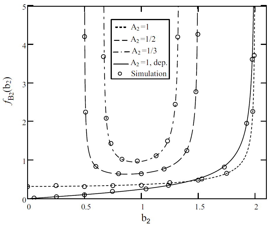
Figure 1: Plot of the pdf’s of examples 1 to 3, $n=2$ with dependent and independent phases, $A_{1}=1$.

(See Figure 1 for a graph of this pdf).

Example 2   Assume that in example 1 above, $\phi_{1}$ and $\phi_{2}$ are dependently distributed with joint pdf

$$f(\phi_{1},\phi_{2})={1\over\pi^{3}}(\phi_{1}+\phi_{2})\hskip 22.76219pt0\leq\phi_{i}\leq\pi.$$ (11)

It can easily be verified that the joint pdf of the corresponding $T_{i}$ random variables is [17]

$$f_{T_{1},T_{2}}(t_{1},t_{2})={8(\tan^{-1}t_{1}+\tan^{-1}t_{2})\over\pi^{3}(1+t_{1}^{2})(1+t_{2}^{2})}\hskip 22.76219pt0\leq t_{i}<\infty\ ..$$ (12)

Then, in this case formula (6) above reduces to

$$P(B_{2}\leq b_{2})=\int_{-\infty}^{\infty}{\bf 1}_{\{|t_{1}|>\alpha\}}\ dt_{1}\int_{-\infty}^{\infty}dt_{2}f_{T_{1},T_{2}}(t_{1},t_{2})+\int_{-\infty}^{\infty}dt_{1}\int_{\bar{a}_{2}}^{\bar{b}_{2}}dt_{2}f_{T_{1},T_{2}}(t_{1},t_{2}).$$ (13)

where the parameter values are as in example 1, except the joint pdf which is given in (12). Calculating the integrals in (13), by methods very similar to example 1 above we obtain

$$F_{B}(b)={4\over\pi^{2}}(\tan^{-1}\alpha)^{2}\hskip 22.76219pt0\leq b\leq 2|A|\ .$$ (14)

Hence, the amplitude pdf for this example is

$$f_{B}(b)={8\over\pi^{2}}{\tan^{-1}\alpha\over\sqrt{(4A^{2}-b^{2})}}\hskip 22.76219pt0\leq b\leq 2|A|\ .$$ (15)

From the pdf (15) it is evident that it has a singularity at $b_{2}=2A$ which can also be seen in Fig. 1, where the pdf is illustrated for $A=1$.

Example 2 also illustrates that formula (6) can find the envelope pdf in the more general, and practically more realistic situations where the phase angles may have any arbitrary joint law, and may not be limited to be independent or be uniform. This example can have applications where the phase angles are correlated, and their probability of occurrence would linearly increase with the angle, e.g. in signal propagation over correlated multipath fading channels, particularly the 2-ray models used for mobile radio channels.

III Envelope separation and its pdf in terms of the joint pdf

In this section we represent the pdf of the envelope, directly in terms of any given joint pdf of the amplitudes and the phase angles in the stochastic sinusoidals sum. First the Envelope Separation Theorem (EST) is presented, which gives a recursive formula for the $n^{th}$ envelope in terms of the $(n-1)^{st}$ envelope and resultant phase angle. This can also be viewed as a type of second cosine theorem. Theorem 2 then derives a new Exact General Envelope Distribution (EGED) formula for the envelope pdf. The advantage of this formula over (6) is that the regions of integration are explicitly determined, however the disadvantage in applications is the complications of dealing with bounded regions of integrations compared to $(-\infty,\infty)$ of $t_{i}$ in (6).

The EST expresses the $n^{th}$ envelope $B_{n}^{2}$ as

$$B_{n}^{2}=B_{n-1}^{2}+A_{n}^{2}+2A_{n}B_{n-1}\cos(\phi_{n}-\theta_{n-1}).$$ (16)

The proof is by separating all the terms involving $A_{n}$ in formula (3), and writing the remaining terms as $B_{n-1}^{2}$ [17].

It can immediately be seen from (16) that, if we assume $\phi_{i}$s to have a special form such that, $\{\xi_{i}\triangleq\phi_{i}-\theta_{i-1},\ i=2...n,\ \ \theta_{1}=\phi_{1}\}$ is an i.i.d. (independent and identically distributed) sequence of random variables, then clearly the sequence $\{B_{i}^{2},\ i=1,2,...\}$ becomes Markovian, and a simple recursive formula can be written for its distribution. This assumption was made by Simon [11], where the $\xi_{i}$s were further assumed to be independently uniformly distributed. Though Simon’s work is interesting, and his formula can be derived as special cases of the results of this paper, however the assumptions are very restrictive on the general model considered here as well as on the scope of practical applications, in particular these assumptions imply that, each received sinusoidal adapts its phase to the resultant phase of all the previous sinusoidals in a special way, which also leads to a particular joint law for the $\phi_{i}$s. Since by our formula (4), Simon’s assumption is equivalent to saying that, $\{\phi_{i},\ i=1\cdots,n\}$ are such that, they satisfy

$$\xi_{i}\buildrel\triangle\over{=}\phi_{i}-\tan^{-1}{\frac{\sum_{j=1}^{i-1}A_{j}\sin\left(\phi_{j}\right)}{\sum_{j=1}^{i-1}A_{j}\cos\left(\phi_{j}\right)}}\sim U(-\pi,\pi)\hskip 42.67912pti=2,\cdots,n$$

and the $\xi_{i}$ s are i.i.d., which are complicated special modelling assumptions about the $\{\phi_{i},\ i=1\cdots,n\}$. Another immediate consequence of Simon’s assumption is that, the phases can never be independent, since, for example under this assumption we would have

$$P(\phi_{2}\leq y/\phi_{1}=x)= P(\phi_{2}-\phi_{1}\leq y-x/\phi_{1}=x)$$ (17)

$$= {{y-x+\pi\over 2\pi}}$$ (18)

$$\neq P(\phi_{2}\leq y)\ .$$

But, alternatively, in the absence of any additional (physical) information to the contrary, it would be more natural and physically meaningful, to assume that each signal’s phase is independent of the others, and is uniformly distributed. Our general formulae allow us to model and solve these cases as well, as special cases. Moreover, at the expense of little extra mathematical complexity, we can still derive recursive formulae in the general independent cases without Simon’s assumptions.

Theorem 2 (Exact General Envelope Density (EGED) via the joint pdf )   Under the assumptions of Theorem 1, if the amplitudes and phases random variables $\mathbf{A}$ and $\mathbf{\Phi}$, have a given general joint pdf $f_{{}_{\mathbf{A},\mathbf{\Phi}}}(\mathbf{a},\mathit{\Phi})\triangleq f_{A_{1}...A_{n},\Phi_{1}...\Phi_{n}}(a_{1},...,a_{n},\phi_{1},...,\phi_{n})$, then the pdf of the envelope $B_{n}$ is given by

$$f_{B_{n}}(b_{n})=2b_{n}E\left\{\left|\sqrt{4A_{n}^{2}B_{n-1}^{2}-(b_{n}^{2}-B_{n-1}^{2}-A_{n}^{2})^{2}}\right|^{-1}1_{\{\left|\Psi_{n}\right|\leq 1,\ \Phi_{n}\in U_{n}\}}\right\}\text{ \ \ }m_{n}\leq b_{n}\leq M_{n}\ ,$$ (19)

where the expectation is with respect to the given joint law $f_{{}_{\mathbf{A},\mathbf{\Phi}}}$, and $\mathbf{1}_{\{.\}}$ denotes the indicator of the set $\{.\}$ and

$$\mathbf{\Psi}_{n}\triangleq\left(\frac{b_{n}^{2}-B_{n-1}^{2}-A_{n}^{2}}{2A_{n}B_{n-1}}\right),\text{ }U_{n}\triangleq\{\alpha_{i},\ |\alpha_{i}|<\pi,i=1,...,4\},\text{ }\alpha_{i}\in\{\theta_{n-1}\pm|\cos^{-1}\Psi_{n}|\mp 2k\pi,\ k=0,1\}\ ,$$ (20)

and the expectation integration is in the $(\bf a,{\it\Phi})$ region where, $\phi_{n}$ can only take the four values listed in the set $U_{n}$, in terms of the remaining integration variables.

Example 3   As an example of the implementation of the EGED formula (19), consider the case $n=3$, and suppose $\phi_{i},\ i=1,2,3$ are independently uniformly distributed in $[-\pi,\pi]$, and the $A_{i}$s are constants. Then, application of formula (19), a change of variable of integration and simplification, shows that if we let

$$f_{\mathbf{A},\mathbf{\Phi}}(\mathbf{a},\mathit{\Phi})=(8\pi^{3})^{-1},\ \ \ \bar{b}_{2}^{2}\triangleq|\mathbf{A}|^{2}+2A_{1}A_{2}\cos(\phi_{1}),\ \ \text{and }\ \ \bar{\psi}_{3}\triangleq\left(\frac{b_{3}^{2}-\bar{b}_{2}^{2}-A_{3}^{2}}{2A_{3}\bar{b}_{2}}\right)\ ,$$ (21)

then we obtain [17]

$$f_{B_{3}}(b_{3})=\left\{\begin{array}[]{cc}\hskip-8.53581pt\hskip-8.53581pt\tfrac{2b_{3}}{\pi^{2}}\int_{0}^{\pi}1_{\{\left|\bar{\psi}_{3}\right|\leq 1\}}\frac{d\phi_{1}}{\sqrt{4A_{3}^{2}\bar{b}_{2}^{2}-(b_{3}^{2}-\bar{b}_{2}^{2}-A_{3}^{2})^{2}}}&m_{3}\leq b_{3}\leq M_{3}\\ 0\text{ \ \ \ \ \ \ \ \ \ \ \ \ \ \ \ \ \ \ \ \ \ \ \ \ \ \ \ \ \ \ \ \ \ \ \ \ \ \ \ \ \ \ \ \ }&\text{otherwise}.\end{array}\right.$$ (22)

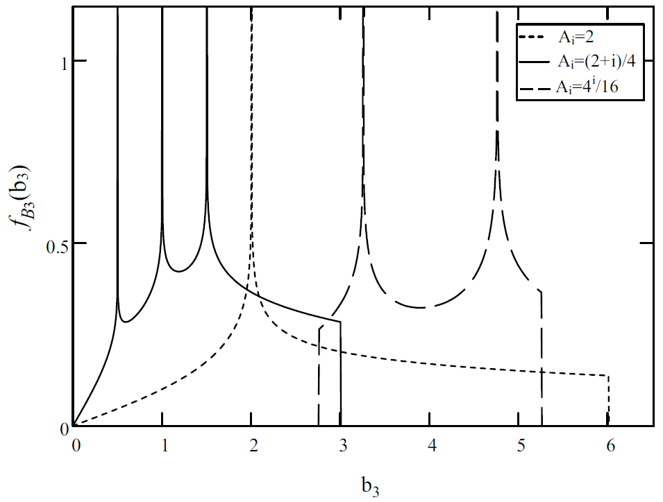
Figure 2: Plot of the pdf’s of example 3, $n=3$, $i=1,2,3$.

Graphs of numerical examples of this pdf are also illustrated in Figure 2 for various amplitude values.

Moreover, when $A_{i}=1,\ i=1,2,3$, the pdf (22) further simplifies to [17]

$$f_{B_{3}}(b_{3})=\left\{\begin{array}[]{cc}\hskip-8.53581pt\hskip-8.53581pt\frac{2b_{3}}{\pi^{2}}\int_{\tilde{m}_{2}}^{\tilde{M}_{2}}\frac{d\phi_{1}}{\sqrt{4\bar{b}_{2}^{2}-(b_{3}^{2}-\bar{b}_{2}^{2}-1)^{2}}}&0\leq b_{3}\leq 3\\ 0\text{ \ \ \ \ \ \ \ \ \ \ \ \ \ \ \ \ \ \ \ \ \ \ \ \ \ \ \ \ \ \ }&\text{otherwise}\ ,\end{array}\right.$$ (23)

where in this case

$\bar{b}_{2}^{2}\triangleq 2+2\cos(\phi_{1})$, $\tilde{M}_{2}\triangleq\left|\cos^{-1}\left((b_{3}-1)^{2}/2-1\right))\right|$, and $\tilde{m}_{2}\triangleq\left|\cos^{-1}(\min(b_{3}+1,2)^{2}/2-1)\right|$.

It follows from formula (23) that in this case the pdf has a singularity at $b_{3}=1$ which can also be observed in the graph of Fig. 2.

Formula (23) can also be written in terms of the EllipticF and EllipticK functions whose numerical values are well tabulated and coded

$$f_{B_{3}}(b_{3})=\frac{{4}Ib_{3}}{\pi^{2}}U\left\{\begin{array}[]{cc}\hskip-22.76219pt\text{EllipticK}(P)-\text{EllipticF}(1/P,P)&0\leq b_{3}\leq 1\\ \text{EllipticK}(P)\text{ \ \ \ \ \ \ \ \ \ \ \ \ \ \ \ \ \ \ \ \ \ \ \ \ \ \ \ \ \ }&1<b_{3}\leq 3\ ,\end{array}\right.\$$ (24)

where

$$I\triangleq\sqrt{-1}\text{, }\ \ \ \ U\triangleq\frac{1}{\left|1-b_{3}\right|\sqrt{(3+b_{3})(1-b_{3})}}\text{, }\ \ \ \ V\triangleq(1+b_{3})^{-{3/2}}(3-b_{3})^{-\frac{1}{2}}\text{,}\ \ \ \ P\triangleq\frac{U}{V}\ ,$$ (25)

and

$$\text{EllipticF}(Q,P)=\int_{0}^{Q}[(1-P^{2}x^{2})(1-x^{2})]^{-\frac{1}{2}}dx,\ \ \ \ \text{EllipticK}(P)=\text{EllipticF}(1,P)\ ,$$ (26)

and formulae (23)-(25) all give the required new amplitude pdf. The pdf given in (23) is illustrated in Fig. 2, which matches the pdf obtained from simulation, also illustrated in Fig. 2.

The pdf for the $n=2$ case of example 3, with different amplitudes $A_{1}$ and $A_{2}$, and independent uniform phases $\phi_{1}$ and $\phi_{2}$, can also be directly obtained from (21) and (22) above, by simply setting $A_{1}=0$, and replacing $b_{3}$ with $b_{2}$, $A_{3}$ with $A_{2}$, and $A_{2}$ with $A_{1}$, and noting that the integrand in (22) becomes independent of $\phi_{1}$, hence giving

$$f_{B_{2}}(b_{2})=\left\{\begin{array}[]{cc}\hskip-5.69054pt\frac{{2b_{2}}}{{\pi\sqrt{4A_{1}^{2}A_{2}^{2}-(b_{2}^{2}-A_{1}^{2}-A_{2}^{2})^{2}}}}\hskip 56.9055ptm_{2}\leq b_{2}\leq M_{2},\\ \hskip-11.38109pt0\text{\hskip 156.49014ptotherwise.}\end{array}\right.$$ (27)

Examples of this pdf are also plotted in Figure 1, where the match with simulation is also observed.

Example 4   As another example of application of the EGED formula (19), consider the $n=4$ case of example 1. Then, application of formula (19), and again a change of variable of integration and simplification, shows that if we let

$f_{{\bf A},{\bf\Phi}}({\bf a},{\it\Phi})=(16\pi^{4})^{-1},\ \ \bar{b}_{3}^{2}\buildrel\triangle\over{=}|{\bf A}|^{2}+2\bigl{[}A_{1}A_{2}\cos(\phi_{1})+A_{2}A_{3}\cos(\phi 2)+A_{1}A_{3}\cos(\phi_{2}-\phi_{1})\bigr{]}$,

and   $\bar{\psi}_{4}\buildrel\triangle\over{=}{b_{4}^{2}-\bar{b}_{3}^{2}-A_{4}^{2}\over 2A_{4}\bar{b}_{3}}$,  then we obtain [17]

$$f_{B_{4}}(b_{4})=\left\{\begin{array}[]{cc}\tfrac{b_{4}}{2\pi^{3}}\int_{-\pi}^{\pi}\int_{-\pi}^{\pi}1_{\{\left|\bar{\psi}_{4}\right|\leq 1\}}\frac{d\phi_{1}d\phi_{2}}{\sqrt{4A_{4}^{2}\bar{b}_{3}^{2}-(b_{4}^{2}-\bar{b}_{3}^{2}-A_{4}^{2})^{2}}}&m_{4}\leq b_{4}\leq M_{4}\\ 0\text{ \ \ \ \ \ \ \ \ \ \ \ \ \ \ \ \ \ \ \ \ \ \ \ \ \ \ \ \ \ \ \ \ \ \ \ \ \ \ \ \ \ \ \ \ \ }&\text{otherwise}\ ,\end{array}\right.$$ (28)

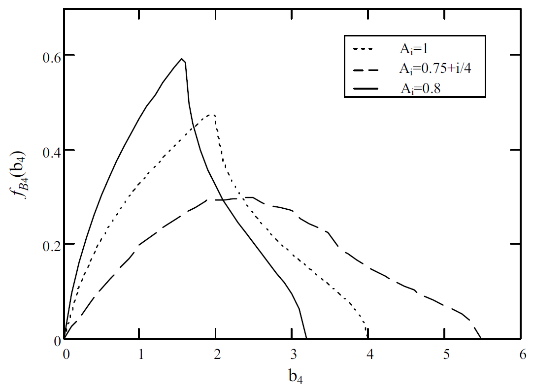
Figure 3: Plot of the pdf’s of example, $n=4$, and $i=1,2,3,4$.

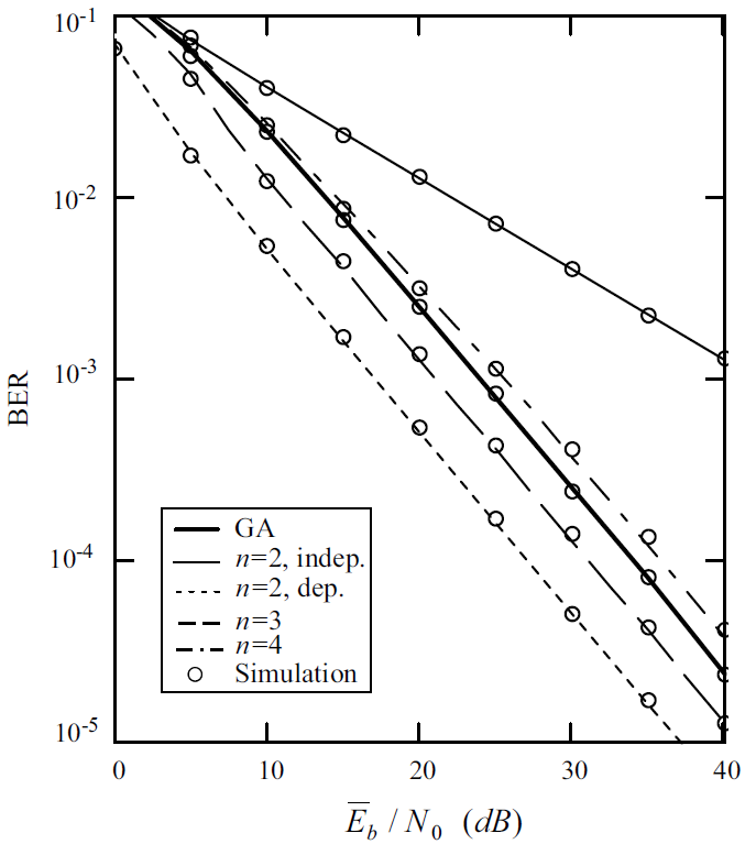
Figure 4: Probability of error for different number of multipath components, via the exact formulae, Gaussian Approximation and simulation.

The pdf (28) is also another hitherto undiscovered pdf, applicable in practical situations such as multiple access processes having one reference user and three interfering users, (see e.g. Fig. 4), multipath channels with four taps, communication systems with cochannel interference, and so on. It is illustrated in Fig. 3, for $A_{i}=1,\ i=1,\cdots,4$. The graph matches that of the pdf obtained from simulation, also illustrated in Fig. 3. In similar fashions we can apply the EGED formula to derive the exact amplitude pdfs for all other values of $n$, in terms of multiple integrals of order $n-2$ of functions of the given parameters.

Example 5  (Random Amplitudes) If the amplitudes are random with the joint density $f_{\bf A}(\bf a)$, and are independent of the phases, then it follows from formula (19) that the envelope pdf, ${\tilde{f}}_{\tilde{B}}(\tilde{b})$, of this case, is the integral of the envelope pdf, $f_{B}(b)$ of the corresponding constant amplitude case, w.r.t. the joint density of the amplitudes, i.e.

$${\tilde{f}}_{\tilde{B}}(\tilde{b})=\int_{-\infty}^{\infty}\hskip-8.53581pt\cdots\int_{-\infty}^{\infty}da_{1}\cdots da_{n}\ f_{\bf A}({\bf a})\ f_{B}(b)$$ (29)

For example the extension of the pdf obtained in (22) of example 3 above, to the random amplitude case is

$${\tilde{f}}_{{\tilde{B}}_{3}}({\tilde{b}}_{3})=\tfrac{2b_{3}}{\pi^{2}}\int_{-\infty}^{\infty}\int_{-\infty}^{\infty}\int_{-\infty}^{\infty}\hskip-8.53581ptda_{1}da_{2}da_{3}f_{\bf A}({\bf a})\int_{0}^{\pi}\frac{1_{\{\left|{\tilde{\psi}}_{3}\right|\leq 1\}}d\phi_{1}}{\sqrt{4a_{3}^{2}\tilde{b}_{2}^{2}-(b_{3}^{2}-\tilde{b}_{2}^{2}-a_{3}^{2})^{2}}}\ \ \ m_{3}\leq b_{3}\leq M_{3}$$ (30)

where $\tilde{b}_{2}$ and $\tilde{\psi}_{3}$, respectively denote $\bar{b}_{2}$ and $\bar{\psi}_{3}$ of (21), with $A_{i}$ replaced with $a_{i}$ for $i=1,2,3$.

For example if the amplitudes ${\bf A}=(A_{1},A_{2},A_{3})$ are jointly Gaussian, with mean vector $\boldsymbol{\mu}$ and covariance matrix $\bf C$, and the phases are distributed as in example 3, and are independent of the amplitudes, then the envelope density in this case is be given by (30), with $f_{\bf A}(\bf a)$ substituted by

$$f_{\bf A}({\bf a})={1\over{2\pi\sqrt{|{\bf C}|2\pi}}}\exp\bigl{[}-{1\over 2}({\bf a}-{\boldsymbol{\mu}})^{T}{\bf C}^{-1}({\bf a}-{\boldsymbol{\mu}})\bigr{]}$$ (31)

For example in example 1 of section II, if the amplitudes are the same normally distributed random variable, with zero mean and variance ${\sigma}^{2}$, then the pdf of the envelope is given by

$$f_{B}(b) ={2\over{\sigma}\pi\sqrt{2\pi}}\int_{-\infty}^{\infty}da{\bf 1}_{\{|a|<b/2\}}{\exp-{1\over 2{\sigma}^{2}}a^{2}\over{\sqrt{4a^{2}-b^{2}}}}$$ (32)

$$={4\over{\sigma}\pi\sqrt{2\pi}}\int_{b/2}^{\infty}da{\exp-{1\over 2{\sigma}^{2}}a^{2}\over{\sqrt{4a^{2}-b^{2}}}}$$ (33)

$$={\sqrt{2}\over{\sigma}\pi\sqrt{2\pi}}\int_{0}^{2}dx{\exp-{b^{2}\over 4{\sigma}^{2}x}\over{x\sqrt{2-x}}}$$ (34)

$$=-{1\over{\sigma}\pi\sqrt{2\pi}}e^{-{1\over 4}c^{2}}K_{0}\bigl{(}{1\over 4}c^{2}\bigr{)}$$ (35)

where the third line in (35) follows from the change of the variable of integration $a^{2}={b^{2}\over 2x}$, and in the last line, $c\buildrel\triangle\over{=}{b\over 2{\sigma}}$, and $K_{0}$ denotes the modified Bessel function of the second kind of order zero.

Example 6 (Mixture of discrete and continuous distributions) The EGED formula (19) can also be applied to the cases where the amplitudes and phases have an arbitrary mixture of discrete and continuous densities. To illustrate this power of the EGED formula, consider a two dimensional example where the amplitudes have an arbitrary joint continuous pdf $f(a_{1},a_{2})$, and are independent of the phases, and assume that the phases are mutually independent, taking only each of the discrete values $0$ or $\pi$, with probability ${1\over 2}$. Thus in this case the EGED formula becomes

$$f_{B}(b)=2bE\left\{\left|2A_{2}A_{1}\sqrt{1-\Psi_{2}}\right|^{-1}1_{\{\left|\Psi_{2}\right|\leq 1,\ \Phi_{2}\in U_{2}\}}\right\}\text{ \ \ }m_{2}\leq b\leq M_{2}\ ,$$ (36)

and $\phi_{1}$ replaces $\theta_{n-1}$ in the definition (20) of the set $U_{2}$. Using the Dirac delta functions we can represent the discrete phase densities and write

$$f_{B}(b)=2b\int_{-\infty}^{\infty}\int_{-\infty}^{\infty}{da_{1}da_{2}f(a_{1},a_{2})\over\left|2a_{2}a_{1}\sqrt{1-\psi_{2}}\right|}{1\over 4}\prod_{i=1}^{2}\int_{-\pi}^{\pi}d\phi_{i}\bigl{[}{\delta}(\phi_{i})+{\delta}(\phi_{i}-\pi)\bigr{]}{\bf 1}_{\{\left|\psi_{2}\right|\leq 1,\ \phi_{2}\in U_{2}\}}$$ (37)

Let $C_{2}\buildrel\triangle\over{=}|\cos^{-1}\psi_{2}|\in[0,\pi]$, and implement the delta functions $[{\delta}(\phi_{1})+{\delta}(\phi_{1}-\pi)\bigr{]}$ into the set $U_{2}$, followed by implementing the delta functions $[{\delta}(\phi_{2})+{\delta}(\phi_{2}-\pi)\bigr{]}$ into the result. The product term in the latter part of (37), which we denote by $\tilde{P}$, will then become

$$\tilde{P} \buildrel\triangle\over{=}\prod_{i=1}^{2}\int_{-\pi}^{\pi}d\phi_{i}\bigl{[}{\delta}(\phi_{i})+{\delta}(\phi_{i}-\pi)\bigr{]}{\bf 1}_{\{|\psi_{2}|\leq 1,\ \phi_{2}\in U_{2}\}}$$ (38)

$$=\int_{-\pi}^{\pi}d\phi_{2}\bigl{[}{\delta}(\phi_{2})+{\delta}(\phi_{2}-\pi)\bigr{]}{\bf 1}_{\{|\psi_{2}|\leq 1\}}\Bigl{[}{\bf 1}_{\{\phi_{2}\in\{\pm C_{2},\ \pm(C_{2}-2\pi)\}\}}+{\bf 1}_{\{\phi_{2}\in\{\pi\pm C_{2},\ \pi\pm(C_{2}-2\pi)\}\}}\Bigr{]}$$ (39)

$$={\bf 1}_{\{\left|\psi_{2}\right|\leq 1\}\}}\Bigl{[}{\bf 1}_{\{C_{2}=0\}}+{\bf 1}_{\{C_{2}=\pi\}}+{\bf 1}_{\{C_{2}=\pi\}}+{\bf 1}_{\{C_{2}=0\}}\Bigr{]}$$ (40)

$$={\bf 1}_{\{\left|\psi_{2}\right|\leq 1\}\}}\Bigl{[}{\bf 1}_{\{\psi_{2}=1\}}+{\bf 1}_{\{\psi_{2}=-1\}}+{\bf 1}_{\{\psi_{2}=-1\}}+{\bf 1}_{\{\psi_{2}=1\}}\Bigr{]}$$ (41)

Substituting the last expression in (41) back into (37) whilst noting the denominator singularity at $\psi_{2}=\pm 1$ we have

$$f_{B}(b)=2b\int_{-\infty}^{\infty}\int_{-\infty}^{\infty}da_{1}da_{2}{f(a_{1},a_{2})\over\left|2a_{2}a_{1}\right|}{1\over 4}{\bf 1}_{\{\left|\psi_{2}\right|\leq 1\}\}}\Bigl{[}2{\delta}(\psi_{2}-1)+2{\delta}(\psi_{2}+1)\Bigr{]}$$ (42)

Now using the formula

$${\delta}(f(x))=\sum_{i=1}^{n}{{\delta}(x-x_{i})\over|f^{\prime}(x_{i})|}$$

where the $x_{i}$ are the real roots of $f(x)$, the delta functions of $\psi_{2}$ can be written in terms of those of $a_{2}$, using the roots of $\psi_{2}=\pm 1$, which are $\{x_{1}=b-a_{1},\ a_{1}\leq b\}$, $\{x_{2}=a_{1}-b,\ a_{1}\geq b\}$, and $x_{3}=a_{1}+b$ respectively. We thus obtain the required envelope pdf from (42)

$$f_{B}(b) ={1\over 2}b\int_{-\infty}^{\infty}\int_{-\infty}^{\infty}da_{1}da_{2}{f(a_{1},a_{2})\over\left|a_{2}a_{1}\right|}\sum_{i=1}^{3}{1\over b}\Bigl{[}|a_{1}x_{i}|{\delta}(a_{2}-x_{i})\Bigr{]}$$ (43)

$$={1\over 2}\Bigl{[}\int_{-\infty}^{b}f(a_{1},b-a_{1})+\int_{b}^{\infty}f(a_{1},a_{1}-b)+\int_{-\infty}^{\infty}f(a_{1},a_{1}+b)\Bigr{]}da_{1}$$ (44)

A simple special case of this example is when the amplitudes are independently negative exponentially distributed, with parameter ${\lambda}$, thus allowing higher probabilities for lower amplitudes, we obtain an interesting envelope pdf

$$f_{B}(b)={1\over 2}{\lambda}e^{-{\lambda}b}({\lambda}b+1)$$

IV Application to BER performance

As an application of the derived formulae, we consider the bit error rate (BER) evaluation of BPSK systems over narrowband multipath fading channels. In such channels, the delay spread $T_{m}$ of a channel is small relative to the inverse signal bandwidth $B^{-1}$ of the transmitted signal, i.e. $T_{m}\ll B^{-1}$. This implies that the delay $\tau_{i}$ associated with the $i$th multipath component $\tau_{i}\leq T_{m}$ $\forall$ $i$, so the baseband signal $s(t)\approx s(t-\tau_{i})$ $\forall$ $i$. The received signal representation with narrowband multipath fading and Gaussian noise in the presence of $n$ multipath components is given by [2][3],

$$r(t)=\sum\limits_{i=1}^{n}\alpha_{i}\cos(2\pi f_{c}t+\phi_{i})+z(t),\text{\ \ \ \ \ \ \ \ }0\leq t<T_{s}$$ (45)

where $\alpha_{i}$ is the amplitude and $\phi_{i}$ is the phase of the $i$th multipath component, respectively, the carrier frequency is denoted as $f_{c}$ and the symbol duration as $T_{s}$. In practice, the amplitudes $\alpha_{i}s$ of the individual multipath components do not fluctuate widely over a local area because the channel characteristics change slowly with respect to $T_{s}$. However, the phases $\phi_{i}s$ vary greatly even for very small values of time delays because the distances traversed by the propagating waves are orders-of-magnitude larger than the wavelength of the carrier frequency. Therefore, the phases are usually modelled as independent random variables uniformly distributed over $[-\pi,\pi]$ [1]-[3]. In such channels, each individual term $\alpha_{i}\cos(2\pi f_{c}t+\phi_{i})$ in (45) is referred to as a specular component.

Using the SAT formula, we can express (45) as $r(t)=B_{n}\cos(\omega t+\theta_{n})+z(t)$ where the amplitude $B_{n}$ is a random variable with a pdf that depends on the value of $n$. A considerable simplification for the channel model is achieved by using the common assumption that $n$ is large and all amplitudes and phases are mutually independent, thus the Central Limit Theorem can be invoked to approximate the received signal as a Gaussian random process, hence the pdf of $B_{n}$ becomes the well-known Rayleigh distribution. However, applying the Gaussian approximation (GA) to the modelling of fading channels that have small number of specular components, will not be accurate enough to describe the effects of the fading process. Thus, the formulae derived in this work can be of great benefit to solve the exact model of the narrowband fading channels, and evaluate the BER of such channels significantly more accurately.

The average bit error probability $P_{B}$ for BPSK in narrowband multipath fading channels can be obtained by integrating the corresponding error probability in AWGN over the fading distribution [1][2],

$$P_{B}=\int_{0}^{\infty}Q\left(\sqrt{2b_{n}^{2}\frac{E_{b}}{N_{0}}}\right)\,f_{B_{n}}(b_{n})\text{ }db_{n}$$ (46)

where $Q\left(\sqrt{2E_{b}/N_{0}}\right)$ is the probability of bit error in AWGN channels. For large $n$, the pdf of $b_{n}$ is Rayleigh distributed and (46) is reduced to a simple closed-form formula [1]. The computation of $P_{B}$ is usually performed versus the average signal-to-noise ratio per bit $\bar{E}_{b}/N_{0}=E\left(b_{n}^{2}\right)E_{b}/N_{0}$, where $E(b_{n}^{2})$ denotes the expected value of $b_{n}^{2}$. For small $n$ values, the pdf of $b_{n}$ is given by (19) which can be substituted in (46) to compute $P_{B}$ for any $n$ value. The analytical and simulation results for $P_{B}$ as a function of $\bar{E}_{b}/N_{0}$ are presented in Fig. $4$ for $n=1,2,3,4,$ the $n=2$ case with dependent phases is also included. All multipath components are assumed to have equal average power. As demonstrated by Fig. $4$, the GA has a large discrepancy which is around $3$ dB for $n=3$, and it is around $1.5$ dB for $n=4$. In the case of $n=2,$ which is known as the Two-Ray model [2], a large difference in $P_{B}$ is observed between the dependent and the independent cases. Such behavior can be understood with the aid of Fig. $1$ which shows that $P(b_{2}<1)$ with independent phases is much larger than that with dependent phases, i.e., the probability that the interference is destructive is much larger when the phases are independent.

V Conclusion

In this paper we considered the open problem of derivation of exact distributions of the envelopes of general stochastic sinusoidal sums, with random amplitudes and phase angles, and its application in an important communication problem. We have seen that, in the most general case, it is possible to derive exact general formulae for the distribution of the resultant envelope in terms of just the given joint distribution of the amplitudes and the phase angles of the signals present in the sum. We derived two such general formulae, EDDHAPT and EGED, depending on the particular applications at hand. Examples showed that implementation of these formulae also lead to new explicit distributions which we applied to compute the exact BER performance of BPSK systems in narrowband fading channels. The extension of these envelope pdf formulae to allow random number of signals is immediate under independence. Under no independence, the extension still follows naturally, but less immediately.

The presented formulae were applied to compute the exact BER performance of BPSK systems in narrowband multipath fading channels with small number of resolvable multipath components. All the simulation results were consistent with the exact theoretical findings, which also showed significant gain in accuracy over the currently popular Gaussian approximation method, particularly for small number of components.

In all cases, the formulae presented in this paper render themselves to accurate and efficient numerical implementations, since at worst they merely involve numerical computation of multiple integrals of known functions, the various algorithms for which are widely available and coded. In some cases the pdfs can be written in terms of known integrals such as Elliptic and Bessel functions. Further numerical implementations and applications may also form part of future work.

VI Appendix

In this appendix we present the proofs of Theorem 1 and Theorem 2. These were first reported in [17], where details of the proofs and other related results may be found.

VI-A Proof of Theorem 1 ( The EDDHAPT formula )

Formula (3) can be written as

$$B_{n}^{2}=\sum_{i=1}^{n}A_{i}^{2}+2A_{n}\sum_{k=1}^{n-1}A_{k}\cos(\phi_{n}-\phi_{k})+2\hskip-8.53581pt\sum_{(n-1)\geq j>k\geq 1}\hskip-8.53581ptA_{j}A_{k}\cos\left(\phi_{j}-\phi_{k}\right)\ .$$ (47)

Expanding the $\cos$ terms and writing in terms of the half-angle tangents we find that

$$B_{n}^{2}=\sum_{i=1}^{n}A_{i}^{2}+2A_{n}\sum_{k=1}^{n-1}{{(1+T_{n}T_{k})^{2}-(T_{n}-T_{k})^{2}}\over(1+T_{n}^{2})(1+T_{k}^{2})}A_{k}+2\hskip-8.53581pt\sum_{(n-1)\geq j>k\geq 1}\hskip-8.53581pt{{(1+T_{j}T_{k})^{2}-(T_{j}-T_{k})^{2}}\over{(1+T_{j}^{2})(1+T_{k}^{2}))}}A_{j}A_{k}$$ (48)

Hence collecting the $T_{n}$ terms in (48), we can write $B_{n}^{2}$ as a quadratic expression in $T_{n}$

$$Q\triangleq(1+T_{n}^{2})(B_{n}^{2}-b_{n}^{2})=aT_{n}^{2}+4A_{n}\bar{S}_{n}T_{n}+(I_{n}+2A_{n}\bar{C}_{n})\ .$$ (49)

The probability on the LHS of (6) is the multiple integral of the pdf over the regions where the quadratic (49) is non-positive. Thus distinguishing between the cases where $a$ or $\Delta_{Q}$ are positive or negative, we have that $Q$ is non-positive only in the union of three disjoint regions within the space $\{\mathbf{a},{\mathbf{t}}\}$, namely the regions $\{\Delta_{Q}>0,a>0,T_{n}\in[\bar{a}_{n},\bar{b}_{n}]\}$, $\{\Delta_{Q}>0,a<0,$ $T_{n}\notin[\bar{b}_{n},\bar{a}_{n}]\}$, and $\{\Delta_{Q}<0,a<0\}$ , where $\bar{a}_{n}$ and $\bar{b}_{n}$ are the roots of $Q$, and $\bar{b}_{n}$ is the larger root in the first region, and vice-versa in the second. Hence

$$P(B_{n}\leq b_{n})= \int_{-\infty}^{\infty}\hskip-8.53581ptd{\bf a}\Biggl{\{}\int_{-\infty}^{\infty}\hskip-8.53581ptd\bar{\bf t}{\bf 1}_{\{\Delta_{Q}>0,a>0\}}\int_{\bar{a}_{n}}^{\bar{b}_{n}}\hskip-8.53581ptdt_{n}f_{{\bf A},{\bf T}}({\bf a,t})+\int_{-\infty}^{\infty}\hskip-8.53581ptd\bar{\bf t}{\bf 1}_{\{\Delta_{Q}>0,a<0\}}\Bigl{\{}\int_{-\infty}^{\bar{b}_{n}}\hskip-8.53581pt+\int_{\bar{a}_{n}}^{\infty}\Bigr{\}}dt_{n}f_{{\bf A},{\bf T}}({\bf a,t})$$ (50)

$$\hskip 22.76219pt+\int_{-\infty}^{\infty}\hskip-8.53581ptd\bar{\bf t}{\bf 1}_{\{\Delta_{Q}<0,a<0\}}f_{{\bf A},\bar{\bf T}}({\bf a},\bar{\bf t})\Biggr{\}}$$ (51)

The second term in (51), which we denote by $I_{2}$, can be written as

$$I_{2} =\int_{-\infty}^{\infty}\hskip-8.53581ptd{\bf a}\Biggl{\{}\int_{-\infty}^{\infty}\hskip-8.53581ptd\bar{\bf t}{\bf 1}_{\{\Delta_{Q}>0,a<0\}}\int_{-\infty}^{\infty}dt_{n}f_{{\bf A},{\bf T}}({\bf a,t})-\int_{-\infty}^{\infty}\hskip-8.53581ptd\bar{\bf t}{\bf 1}_{\{\Delta_{Q}>0,a<0\}}\int_{\bar{b}_{n}}^{\bar{a}_{n}}\hskip-8.53581ptdt_{n}f_{{\bf A},{\bf T}}({\bf a,t})\Biggr{\}}$$ (52)

$$=\int_{-\infty}^{\infty}\hskip-8.53581ptd{\bf a}\Biggl{\{}\int_{-\infty}^{\infty}\hskip-8.53581ptd\bar{\bf t}{\bf 1}_{\{\Delta_{Q}>0,a<0\}}f_{{\bf A},\bar{\bf T}}({\bf a},\bar{\bf t})+\int_{-\infty}^{\infty}\hskip-8.53581ptd\bar{\bf t}{\bf 1}_{\{\Delta_{Q}>0,a<0\}}\int_{\bar{a}_{n}}^{\bar{b}_{n}}\hskip-8.53581ptdt_{n}f_{{\bf A},{\bf T}}({\bf a,t})\Biggr{\}}$$ (53)

Substituting the RHS of (53), into (51) for $I_{2}$, and combining the integrals, we obtain (6) and the proof of the Theorem is complete  

Remark  Note that in the regions where $a=0$ and/or ${\Delta}_{Q}=0$, the probability measures are zero, hence these cases need not be included in the regions of integration.

VI-B Proof of Theorem 2 (The EGED formula )

The proof is by a method which we call The ($n-1$)-Conditioning Method, where we calculate the cdf of $B_{n}^{2}$ by conditioning on the value of the random vector $(\bf A,\bar{\bf\Phi})$, where $\bar{\bf\Phi}$ denotes the vector $({\bf\Phi}_{1},...,{\bf\Phi}_{n-1})$. We obtain

$$P\bigl{(}B^{2}_{n}\leq b_{n}^{2}\bigr{)}=\int_{-\infty}^{\infty}\hskip-8.53581ptd{\bf a}\int_{-\pi}^{\pi}d{\it\bar{\Phi}}\ P\Bigl{(}\cos(\Phi_{n}-\theta_{n-1})\leq\psi_{n}/{\bf a},{\it\bar{\Phi}}\Bigr{)}f_{{}_{{}_{{\bf A},\bar{\bf\Phi}}}}({\bf a},{\it\bar{\Phi}})\ ,$$ (54)

where we have used the EST formula (16), ${\it\bar{\Phi}}$ denotes the vector $(\phi_{1},...,\phi_{n-1})$, and without loss of generality $a_{n}$ is assumed to be positive (see the remark below), and

$$\psi_{n}\buildrel\triangle\over{=}\Bigl{(}{b_{n}^{2}-b_{n-1}^{2}-a_{n}^{2}\over 2a_{n}b_{n-1}}\Bigr{)}\ .$$ (55)

Taking inverse $\cos$ within the probability integrand of (54), while noting that $(\Phi_{n}-\theta_{n-1})\in(-2\pi,2\pi)$, we obtain

$$P\bigl{(}B^{2}_{n}\leq b_{n}^{2}\bigr{)}=\int_{-\infty}^{\infty}\hskip-8.53581ptd{\bf a}\int_{-\pi}^{\pi}\hskip-8.53581ptd{\it\bar{\Phi}}P\Bigl{(}|\cos^{-1}\bar{\psi}_{n}|+|\theta_{n-1}|\leq|\Phi_{n}|\leq 2\pi-|\cos^{-1}\bar{\psi}_{n}|+|\theta_{n-1}|/{\bf a},{\it\bar{\Phi}}\Bigr{)}f_{{}_{{}_{{\bf A},\bar{\bf\Phi}}}}({\bf a},{\it\bar{\Phi}})$$ (56)

where $\Phi_{n}$ and $\theta_{n-1}$ carry the same sign, and the function

$$\bar{\psi}_{n}=\left\{\begin{array}[]{cc}\psi_{n}&|\psi_{n}|\leq 1\\ \hbox{sign}(\psi_{n})&\text{otherwise}\ ,\end{array}\right.$$

ensures that the $\cos^{-1}$ function is well-defined. Note that, as required by (54), when $\psi_{n}\geq 1$ or $\leq-1$, the RHS of (56) takes the values 1 and $0$ respectively. Now writing (56) in terms of the conditional cdf $F_{{}_{\Phi_{n}/{\bf A},\bar{\bf\Phi}}}(\phi_{n})$ of $\Phi_{n}$, given that $({\bf A},\bar{\bf\Phi})=({\bf a},{\it\bar{\Phi}})$, which we simply denote by $\tilde{F}_{n}$, and letting $C_{k}(\bar{\psi}_{n})\buildrel\triangle\over{=}|\cos^{-1}\bar{\psi}_{n}|-2k\pi$, we obtain

$$P\bigl{(}B^{2}_{n}\leq b_{n}^{2}\bigr{)}=\int_{-\infty}^{\infty}\hskip-8.53581ptd{\bf a}\int_{-\pi}^{\pi}\hskip-8.53581ptd{\it\bar{\Phi}}\Bigl{[}\sum_{k=0}^{1}\bigl{\{}\tilde{F}_{n}(-C_{k}(\bar{\psi}_{n})+\theta_{n-1})-\tilde{F}_{n}(C_{k}(\bar{\psi}_{n})+\theta_{n-1})\bigr{\}}\Bigr{]}f_{{}_{{}_{{\bf A},\bar{\bf\Phi}}}}({\bf a},{{\it\bar{\Phi}}})\ .$$ (57)

While noting that, $f_{B_{n}}(b_{n})=2b_{n}f_{B_{n}^{2}}(b_{n}^{2})$, we differentiate (57) with respect to $b_{n}^{2}$ to get the pdf. The derivative of $\bar{\psi}_{n}$ w.r.t. $b_{n}^{2}$ yields the function $\tilde{\bf 1}\buildrel\triangle\over{=}{\bf 1}_{\bigl{\{}|\psi_{n}|\leq 1\bigr{\}}}$ into the integrand, which is followed by $\tilde{f}_{n}$, the conditional pdf of $\Phi_{n}$

$$f_{B_{n}}(b_{n})=2b_{n}\int_{-\infty}^{\infty}\hskip-8.53581ptd{\bf a}\int_{-\pi}^{\pi}\hskip-8.53581ptd{\it\bar{\Phi}}\ \tilde{\bf 1}\Bigl{[}\sum_{k=0}^{1}\bigl{\{}\tilde{f}_{n}(-C_{k}(\psi_{n})+\theta_{n-1})+\tilde{f}_{n}(C_{k}(\psi_{n})+\theta_{n-1})\bigr{\}}\Bigr{]}V(\psi_{n})f_{{}_{{}_{{\bf A},\bar{\bf\Phi}}}}({\bf a},{{\it\bar{\Phi}}})$$ (58)

where $V(\psi_{n})\buildrel\triangle\over{=}(2a_{n}b_{n-1}\sqrt{1-{\psi}_{n}^{2}}\bigr{)}^{-1}=-{\partial|\cos^{-1}(\psi_{n})|\over\partial b^{2}_{n}}$. Note that $\bar{\psi}_{n}$ no longer needs to replace $\psi_{n}$ within the integrands in (58), since now the function $\tilde{\bf 1}$ forces the integrand to zero when $\psi_{n}$ is outside the range $[-1,1]$, which is as required by the fact that the probability sum in (57) takes the constant values of 1 or 0, for all $\psi_{n}\notin[-1,1]$ (see also (54)), hence its derivative within the integrand of (58) should be zero in this region. The product of $\tilde{f}_{n}$ and the marginal pdf $f_{{}_{{}_{{\bf A},\bar{\bf\Phi}}}}({\bf a},{{\it\bar{\Phi}}})$ in the integrand of (58), gives the joint pdf $f_{{\bf A},{\bf\Phi}}({\bf a},{\it\Phi})$, hence we have

$$f_{B_{n}}(b_{n}) =2b_{n}\int_{-\infty}^{\infty}\hskip-8.53581ptd{\bf a}\int_{-\pi}^{\pi}\hskip-8.53581ptd{\it\bar{\Phi}}\ \tilde{\bf 1}\Bigl{[}\sum_{k=0}^{1}\bigl{\{}f_{{\bf A},{\bf\Phi}}({\bf a},{{\it\bar{\Phi}}},-C_{k}(\psi_{n})+\theta_{n-1})+f_{{\bf A},{\bf\Phi}}({\bf a},{{\it\bar{\Phi}}},C_{k}(\psi_{n})+\theta_{n-1})\bigr{\}}\Bigr{]}V(\psi_{n})$$ (59)

$$=2b_{n}\int_{-\infty}^{\infty}\hskip-8.53581ptd{\bf a}\int_{-\pi}^{\pi}\hskip-8.53581ptd{\it\Phi}\ \tilde{\bf 1}\Bigl{[}\sum_{k=0}^{1}\Bigl{\{}{\bf 1}_{\bigl{\{}\phi_{n}=-C_{k}(\psi_{n})+\theta_{n-1}\bigr{\}}}+{\bf 1}_{\bigl{\{}\phi_{n}=C_{k}(\psi_{n})+\theta_{n-1}\bigr{\}}}\Bigr{\}}\Bigr{]}V(\psi_{n})f_{{\bf A},{\bf\Phi}}({\bf a},{\it\Phi})\ .$$ (60)

Finally writing (60) in terms of the expectation with respect to the given joint law $f_{{}_{{\bf A},{\bf\Phi}}}({\bf a},{\it\Phi})$ we obtain (19) and the proof of Theorem 2 is complete.  

Remark    Note that identical steps prove Theorem 2 for the region of integration where $a_{n}$ is negative, as 1 minus the probability in the integrand of (57) is obtained, which after differentiation gives the same result with a negative sign, which changes to the positive sign, by replacing $a_{n}$ with $-|a_{n}|$ in front of the function $V(\psi_{n})$. Hence, for all $a_{n}$, (60) holds with, $|a_{n}|$ replacing $a_{n}$ in front of $V(\psi_{n})$, hence formula (19) follows.

Figure 5: Probability of error for different number of multipath components, via the exact formulae, Gaussian Approximation and simulation.

References

- [1] J. G. Proakis, Digital Communications, McGraw-Hill, 2001.
- [2] A. J. Goldsmith, Wireless Communications, New York, Cambridge University Press, 2005.
- [3] T. S. Rappaport, Wireless Communications Principles and Applications, New Jersy, Prentice Hall, 2002.
- [4] K. Teh, A. Kot, and K. Li, “Multitone jamming rejection of FFH/BFSK spread-spectrum system over fading channels,” IEEE Trans. Commun., vol. 46, , pp. 1050-1057, Aug. 1998.
- [5] K. Choi an K. Cheun, “Performance of asynchronous slow frequency-hop multiple-access networks with MFSK modulation,” IEEE Trans. Commun., vol 48, pp. 298-307, Feb. 2000.
- [6] A. Al-Dweik and F. Xiong, “Frequency-hopped multiple access communications with noncoherent M-ary OFDM-ASK, IEEE Trans. Commun., vol. 51, pp. 33-36, Jan. 2003.
- [7] N. C. Beaulieu and J. Cheng, “Precise error-rate analysis of bandwidth-efficient BPSK in Nakagami fading channels,” IEEE Trans. Commun., vol. 52, pp. 149-158, Jan. 2004.
- [8] S. H. Kim and S. W. Kim, “Frequency-hopped multiple-access communications with multicarrier on-off keying in Rayleigh fading channels,” IEEE Trans. Commun., vol. 48, pp. 1692-1701, Oct. 2000.
- [9] S. O. Rice, “Probability distributions for noise plus several sine waves–The problem of computation,” IEEE Trans. Commun., COM-22, pp. 851-853, Jun. 1974.
- [10] J. Kluyver, “A local probability problem,” Nederlande Akademie van Wetenschap, 8, pp. 341-350, 1906.
- [11] M. K. Simon, “On the probability density function of the squared envelope of a sum of random vectors,” IEEE Trans. Commun., COM-33, pp. 993-996, Sept. 1985.
- [12] C. W. Helstrom, “Distribution of the sum of two sine waves and Gaussian noise,” IEEE Trans. Inform. Theory, vol. 38, pp. 186-191, Jan. 1992.
- [13] C. W. Helstrom, “Distribution of the envelope of a sum of random sine waves and Gaussian noise,” IEEE Trans. Aerosp. Electron. Syst., vol. 35, pp. 594-601, Apr. 1999.
- [14] P. Beckmann and A. Spizzichino, The Scattering of Electromagnetic Waves From Rough Surfaces, 2nd ed. Boston, MA: Artech House, 1987.
- [15] S. M. Zabin and G. A. Wright, “Nonparametric density estimation and detection in impulsive interference channels-Part I: Estimators,” IEEE Trans. Commun., vol. 42, pp. 1684-1697, 1994.
- [16] A. Abdi, H. Hashemi, and S. Nader-Esfahani, “On the PDF of the sum of random vectors,” IEEE Trans. Commun., vol. 48, pp. 7-12, Jan. 2000.
- [17] Y. Maghsoodi ”Exact distributions of envelopes of sums of stochastic sinusoids with general random amplitudes and phases,” Working paper, Scinance Analytics, Nov. 2004.
- [18] Y. Maghsoodi and A. Al-Dweik, ”Error-Rate Analysis of FHSS Networks Using Exact Envelope Characteristic Functions of Sums of Stochastic Signals,” in IEEE Transactions on Vehicular Technology, vol. 57, no. 2, pp. 974-985, March 2008.
- [19] A. Al-Dweik and B. Sharif, ”Exact Performance Analysis of Synchronous FH-MFSK Wireless Networks,” in IEEE Transactions on Vehicular Technology, vol. 58, no. 7, pp. 3771-3776, Sept. 2009.
- [20] A. Al-Dweik, B. Sharif and C. Tsimenidis, ”Accurate BER Analysis of OFDM Systems Over Static Frequency-Selective Multipath Fading Channels,” in IEEE Transactions on Broadcasting, vol. 57, no. 4, pp. 895-901, Dec. 2011.