Temperature-field phase diagrams of one-way quantum work deficit in two-qubit XXZ spin systems

Abstract

The spin-1/2 XXZ chain in a uniform magnetic field at thermal equilibrium is considered. For this model, we give a complete classification of all qualitatively different phase diagrams for the one-way quantum work (information) deficit. The diagrams can contain regions (phases, fractions) with both stationary and variable (state-dependent) angles of optimal measurement. We found cases of phase diagrams in which the sizes of regions with the variable optimal measurement angle are large and perhaps such regions can be detected experimentally. We also established a relationship between the behavior of optimal measurement angles near the boundaries separated different regions and Landau’s theory of phase transitions of the second and first kind.

1 Introduction

Quantum correlations have foundational interest and are an essential resource for quantum information and computational technologies. There are many measures of quantum correlations. One of the most important places among them belongs to the quantum discord and one-way quantum work deficit MBCPV12 ; Str15 ; ABC16 ; FPA17 ; BDSRSS18 . It is significant that the concept of these correlations, as opposed to others, is introduced through measurements and therefore is consistent with the fundamental requirement: “Unless a thing can be defined by measurement, it has no place in a theory” FLS64 . These words repeat the idea of Heisenberg’s 1925 paper H25 . (In this connection, see, e.g., W14 .)

The quantum discord ${\cal Q}$ for a bipartite system $AB$ is defined as the minimum difference between the quantum generalizations of symmetric ($I$) and asymmetric looking ($J$) versions of the classical mutual information: ${\cal Q}=\min_{\{{\rm\Pi}_{k}\}}(I-J)$, where $\{{\rm\Pi}_{k}\}$ is the measurement performed on one of the two subsystems (say, on $B$) Z00 ; OZ02 ; HV01 ; V17 . One can also rewrite this definition in equivalent form as the minimum difference between the quantum conditional entropy after a local measurement (Zurek’s definition Z00 , see also L73 ), $S(A|B_{\{{\rm\Pi}_{k}\}})$, and quantum pseudo-conditional entropy $S(A|B)=S(A,B)-S(B)$; that is, ${\cal Q}=\min_{\{{\rm\Pi}_{k}\}}S(A|B_{\{{\rm\Pi}_{k}\}})-S(A|B)$. Quantum discord equals zero for the classically correlated states and coincides the quantum entanglement for the pure states.

The quantum work deficit is a measure of quantum correlation originated from the thermodynamics view point. In general, it is defined as the minimum difference between the thermodynamic work ${\cal W}$ which can be extracted from a heat bath using operations on the entire quantum system and the largest amount of work $W$ drawn from the same heat bath by manipulating only the local parts of composite system; in other words, the work deficit $\rm\Delta$ is the amount of potential work which cannot be extracted under local operations because of quantum correlations OHHH02 ; HHHHOSS03 ; HHHOSSS05 . Exist several forms of deficit depending on the type of communication allowed between parts $A$ (Alice) and $B$ (Bob). If the bipartite state $\rho_{AB}$ is shared by Alice and Bob and, for example, Bob performs a single von Neumann measurement on his local subsystem and using classical communication sends the resulting state to Alice that extracts the maximum amount of work $W$ from the new entire state then the dimensionless quantity ${\rm\Delta}=\min_{\{{\rm\Pi_{k}}\}}({\cal W}-W)/T$ is called the one-way quantum work deficit; $T$ is the temperature (in energy units) of the common bath.

In spite of quite different conceptual sources, the one-way deficit and discord coincide, contrary to the entanglement, in considerably more general cases. They are identical for the Bell-diagonal (and hence Werner) states and even for the two-qubit X states with one zero Bloch vector if the local measurement is performed on a qubit with the vanished Bloch vector YF16 . On the other hand, the one-way quantum deficit and discord exhibit, generally speaking, different quantitative and even qualitative behavior in more general cases. As a result, we now do not know what value of quantum correlation is correct. This situation is similar to the following: “’a moo must be three goos’, when nobody knows what a moo or a goo is” F65 .

Two following key properties play the crucial roll in our approach. First, for the X quantum states, the optimization of both quantum discord and one-way deficit over the projectors $\{{\rm\Pi}_{k}(\theta,\phi)\}$ can be worked out exactly over the azimuthal angle $\phi$ and therefore only one optimization procedure, in the polar angle $\theta\in[0,\pi/2]$, remains relevant LXSW10 ; CRC10 ; VR12 ; YWF16 ; Y18 ; Y19 . Thus, the non-optimized discord and one-way deficit are the functions of one variable only: $Q=Q(\theta)$ and $\Delta=\Delta(\theta)$, respectively. The second remarkable property is that the first derivatives of named functions with respect to the argument $\theta$ equal zero at both endpoints $\theta=0$ and $\pi/2$ by any choice of state parameters. This is proved by direct calculations.

The optimal measurement angle for the Bell-diagonal states is achieved always on the border of the interval $[0,\pi/2]$, i.e., at the limiting points 0 or $\pi/2$. However, for the more general X states, the optimal measurement angle can also happen inside the open interval $(0,\pi/2)$ LMXW11 ; CZYYO11 ; H13 . In turn, this can lead to the existence of new branch (phase, fraction) of the piecewise-defined quantum correlation function, namely, the phase with the interior, state-dependent (variable) optimal measurement angle: $Q_{\theta^{*}}$ for the quantum discord Y14 ; Y14a ; Y15 ; Y17 and $\Delta_{\vartheta}$ for the one-way quantum work deficit YWF16 ; Y18 ; Y19 .

An observation made by the author Y14 ; Y14a ; Y15 is that the quantum discord function $Q(\theta)$ is unimodal in the open interval $(0,\pi/2)$. Then from topological reasoning it follows that the boundaries between the different fractions (phases) can be found from conditions of vanishing the second derivatives with respect to the angle $\theta$ at the endpoints: $Q^{\prime\prime}(0)=0$ and $Q^{\prime\prime}(\pi/2)=0$. These equations are confirmed now for various subclasses of X states Y15 ; Y17 . The same is valid for the one-way deficit function. Moreover, the measurement-dependent deficit $\Delta(\theta)$ can also exhibit in some cases the bimodal behavior, i.e., it can have two interior extrama: one minimum and one maximum. As a result, this can lead to the new mechanism of formation of the boundary between phases, namely, via finite jumps of optimal measured angle from the endpoint to the interior minimum or vice versa Y18 ; Y19 .

This paper is devoted to the systematic classification of all possible temperature-field phase diagrams for the one-way quantum work deficit in spin-1/2 XXZ dimers. In Sect. 2, the required equations are given for constructing the phase diagrams. Then, in Sect. 3 we solve the corresponding equations, graphically present a complete set of phase diagrams for all qualitatively distinguishable cases, and describe their properties in detail. Finally, in Sect. 4, our main results are summarized and some possible avenues for the future researches are given.

2 Formalism

We will study the structures of piecewise-defined quantum correlation function, namely, the one-way quantum deficit, for the two-site spin-1/2 XXZ chain under a uniform external field $B$ at the temperature $T$.

2.1 Hamiltonian, density matrix, and pre-measurement entropy

Let us consider a composite system $AB$ with the Hamiltonian

$${\cal H}=-\frac{1}{2}[J(\sigma_{x}^{A}\sigma_{x}^{B}+\sigma_{y}^{A}\sigma_{y}^{B})+J_{z}\sigma_{z}^{A}\sigma_{z}^{B}]-\frac{1}{2}B(\sigma_{z}^{A}+\sigma_{z}^{B}),$$ (1)

where $J$ and $J_{z}$ are the coupling constants and $\sigma_{x}^{A,B}$, $\sigma_{y}^{A,B}$, and $\sigma_{z}^{A,B}$ the Pauli spin matrices at sites $A$ and $B$, respectively.

The energy levels of this Hamiltonian equal

$$E_{1,2}=-\frac{1}{2}J_{z}\pm B,\qquad E_{3,4}=\frac{1}{2}J_{z}\pm J$$ (2)

and consequently the partition function $Z=\sum_{i}\exp(-E_{i}/T)$ is given as

$$Z=2\biggl{(}e^{J_{z}/2T}\cosh\frac{B}{T}+e^{-J_{z}/2T}\cosh\frac{J}{T}\biggl{)}.$$ (3)

The function $Z(T,B)$ is invariant under the replacements both $J\to-J$ and $B\to-B$.

The Helmholtz free energy equals ${\cal F}(T,B)=-T\ln Z$ and hence the ordinary thermodynamic entropy $S=-\partial{\cal F}/\partial T$ is expressed for the system (1) by equation

$$S(T,B)=-\frac{1}{Z}\biggl{[}\frac{B+J_{z}/2}{T}\exp\left(\frac{B+J_{z}/2}{T}\right)-\frac{B-J_{z}/2}{T}\exp\left(-\frac{B-J_{z}/2}{T}\right)$$

$$+\frac{J-J_{z}/2}{T}\exp\left(\frac{J-J_{z}/2}{T}\right)-\frac{J+J_{z}/2}{T}\exp\left(-\frac{J+J_{z}/2}{T}\right)\biggr{]}+\ln Z.$$ (4)

The Gibbs density matrix, $\rho_{AB}=\exp(-{\cal H}/T)/Z$, has the structure

$$\rho_{AB}=\left(\begin{array}[]{cccc}a&&&\\ &b&v&\\ &v&b&\\ &&&d\end{array}\right).$$ (5)

Quantum correlations, as known (see, e.g, Ref. MBCPV12 ), must be invariant under any local unitary transformations. Take the local unitary transformation

$$u=e^{i\pi\sigma_{z}/4}\otimes e^{-i\pi\sigma_{z}/4}=\left(\begin{array}[]{cccc}1&&&\\ &i&&\\ &&-i&\\ &&&1\end{array}\right).$$ (6)

It is easy to check that the action of this transformation on the density matrix (5) changes the sign of the off-diagonal entries, i.e., the matrix $u\rho_{AB}u^{+}$ is equal to the right side of Eq. (5) in which $v\to-v$. Thus the density matrix can be brought to the form with real non-negative values for all entries (more details for the general X density matrices can be found, for example, in Refs. Y14 ; Y14a ). As a result, the matrix elements of density matrix (5) can be written as

$$a=\frac{1}{Z}\exp[(J_{z}/2+B)/T],\quad b=\frac{1}{Z}e^{-J_{z}/2T}\cosh(J/T),$$

(7)

$$d=\frac{1}{Z}\exp[(J_{z}/2-B)/T],\quad v=\frac{1}{Z}e^{-J_{z}/2T}\sinh(|J|/T).$$

So, all properties of the system under question do not depend on the sign of constant $J$, i.e., both ferro- and antiferro-interactions in transverse directions of spin space lead to the same results.

Eigenvalues of density matrix $\rho_{AB}$ are equal to

$$\lambda_{1}=a,\quad\lambda_{2}=d,\quad\lambda_{3,4}=b\pm v$$ (8)

or, in an explicit form,

$$\lambda_{1,2}=\frac{1}{Z}\exp[(J_{z}/2\pm B)/T],\qquad\lambda_{3,4}=\frac{1}{Z}\exp[-(J_{z}/2\pm|J|)/T].$$ (9)

The von Neumann entropy before measurement is

$$S(\rho_{AB})\equiv-{\rm Tr}\rho_{AB}\ln\rho_{AB}=-a\ln a-d\ln d-(b+v)\ln(b+v)-(b-v)\ln(b-v).$$ (10)

After inserting expressions for the quantities $a$, $b$, $d$, and $v$ this relation returns to Eq. (2.1).

2.2 Post-measurement entropy and one-way deficit

We now pursue a consideration of one-way quantum work deficit which was begun in Introduction. The maximum amount of useful work that can be extracted from the heat bath via working body (substance) in the state $\rho$ is given as OHHH02 ; HHHHOSS03 ; HHHOSSS05 (see also MBCPV12 ; Str15 ; ABC16 )

$$w=T(\log d_{H}-S(\rho)),$$ (11)

where $S(\rho)=-{\rm tr}(\rho\log\rho)$ is the entropy of state $\rho$ and $d_{H}$ the dimension of Hilbert space in which the density operator $\rho$ acts. Applying this general relation to the states before and after Bob’s measurement one comes to the following working equation for the one-way quantum work (information) deficit HHHOSSS05 (see also, e.g., MBCPV12 ; CCR15 )

$${\rm\Delta}=\min_{\{\rm\Pi_{k}\}}S(\tilde{\rho}_{AB})-S(\rho_{AB}),$$ (12)

where

$$\tilde{\rho}_{AB}\equiv\sum_{k}p_{k}\rho^{k}_{AB}=\sum_{k}({\rm I}\otimes{\rm\Pi}_{k})\rho_{AB}({\rm I}\otimes{\rm\Pi}_{k})^{+}$$ (13)

is the weighted average of post-measured states

$$\rho^{k}_{AB}=\frac{1}{p_{k}}({\rm I}\otimes{\rm\Pi}_{k})\rho_{AB}({\rm I}\otimes{\rm\Pi}_{k})^{+}$$ (14)

with the probabilities

$$p_{k}={\rm Tr}({\rm I}\otimes{\rm\Pi}_{k})\rho_{AB}({\rm I}\otimes{\rm\Pi}_{k})^{+}.$$ (15)

Thus, the one-way quantum work deficit equals the minimal increase of entropy after nonselective orthogonal projective measurements on one party of the bipartite system. Notice that the projective measurements increase entropy (but generalized measurements can decrease it); the proof is based on Klein’s inequality K31 ; NC10 .

So, like the quantum discord, the one-way deficit is non-negative quantity. For the two-qubit systems, the entropies can vary from zero to two bits while the one-way deficit may change its value from zero to one bit only.

As a matter of fact, the pre-measurement entropy $S$ in the expression for the one-way deficit, Eq. (12), plays a roll of trivial shift. Therefore, below we will stress attention mainly on the post-measurement entropies: non-optimized $\tilde{S}(\theta)=S(\tilde{\rho}_{AB})$ and optimized $\tilde{\cal S}=\min_{\theta}S(\tilde{\rho}_{AB})$ ones.

Further, operators ${\rm\Pi}_{k}$ in Eq. (13) are two projectors ($k=0,1$)

$${\rm\Pi}_{k}=V\pi_{k}V^{+},$$ (16)

where $\pi_{k}=|k\rangle\langle k|$ [i.e., $\pi_{0,1}=(1\pm\sigma_{z})/2$] and transformations $\{V\}$ belong to the special unitary group $SU_{2}$. Rotations $V$ are parametrized by two angles $\theta$ and $\phi$ (polar and azimuthal, respectively):

$$V=\left(\begin{array}[]{cc}\cos(\theta/2)&e^{i\phi}\sin(\theta/2)\\ \sin(\theta/2)&-e^{i\phi}\cos(\theta/2)\end{array}\right)$$ (17)

with $0\leq\theta\leq\pi$ and $0\leq\phi<2\pi$.

Solving eigenproblem for the density matrix ${\tilde{\rho}}_{AB}$ defined by Eqs. (5), (2.1), (13), and (17) we get its eigenvalues

$$\Lambda_{1,2}=\frac{1}{4}[\![1+(a-d)\cos\theta\pm\{[a-d+(1-4b)\cos\theta]^{2}+4v^{2}\sin^{2}\theta\}^{1/2}]\!]$$

(18)

$$\Lambda_{3,4}=\frac{1}{4}[\![1-(a-d)\cos\theta\pm\{[a-d-(1-4b)\cos\theta]^{2}+4v^{2}\sin^{2}\theta\}^{1/2}]\!].$$

It is seen that the azimuthal angle $\phi$ has dropped out from the given expressions. This is due to the fact that one pair of anti-diagonal entries of the density matrix (5) vanishes. Moreover, it is clear that every $\Lambda_{i}$ is invariant under the transformation $v\to-v$ without replacement $v$ by $|v|$. Using Eqs. (2.2) we arrive at the post-measured entropy (entropy after measurement)

$$\tilde{S}(\theta;T,B)\equiv S(\tilde{\rho}_{AB})=h_{4}(\Lambda_{1},\Lambda_{2},\Lambda_{3},\Lambda_{4}),$$ (19)

where $h_{4}(x_{1},x_{2},x_{3},x_{4})=-\sum_{i=1}^{4}x_{i}\ln x_{i}$, with the additional condition $x_{1}+x_{2}+x_{3}+x_{4}=1$, is the quaternary entropy function. Notice that function $\tilde{S}$ of argument $\theta$ is invariant under the transformation $\theta\to\pi-\theta$ therefore it is enough to consider the values for which $\theta\in[0,\pi/2]$.

Completing this subsection we return to the second key property of non-optimized one-way deficit which was announced in Introduction. Simple calculations show that the first derivatives of post-measurement entropy, Eqs. (2.2) and (19), with respect to the angle $\theta$ identically equal zero at both endpoints $\theta=0$ and $\pi/2$ for any choice of $a$, $b$, $d$, and $v$:

$${\tilde{S}}^{\prime}(0)\equiv 0,\quad{\tilde{S}}^{\prime}(\pi/2)\equiv 0$$ (20)

and consequently $\Delta^{\prime}(0)\equiv 0$ and $\Delta^{\prime}(\pi/2)\equiv 0$.

2.3 Piecewise-analytical-numerical formula for the one-way quantum work deficit

2.3.1 Branch $\tilde{S}_{0}$

Using Eqs. (2.2) and (19) we find the post-measurement entropy function by $\theta=0$:

$$\tilde{S}_{0}(T,B)\equiv\tilde{S}(0;T,B)=-a\ln a-d\ln d-2b\ln b.$$ (21)

This is a branch of entropy with the stationary optimal measurement angle equaled zero.

The entropy (21) coincides the entropy of diagonal part of the density matrix (5), i.e., entropy of the Gibbs density matrix for the spin system (1) with switched-off (fully suppressed) transverse interactions, $\tilde{\rho}_{AB}|_{J=0}={\rm diag}[a,b,b,d]$. This state corresponds to a purely classical, Ising system. In other words, the nonselective $\sigma_{z}$-measurement $\{{\rm\Pi}_{k}=\pi_{k}\ |\ k=0,1\}$ erases coherence (all non-diagonal terms) from the original density matrix. After such a measurement, the entropy increases: $\tilde{S}_{0}(T,B)\geq S(T,B)$. This is in agreement with a relation $S(\rho_{diag})\geq S(\rho)$ ($\rho_{diag}$ is the diagonal part of arbitrary density matrix $\rho$) that follows from the Klein inequality NC10 (see also F72 ).

Notice that the entropy (21) as well as the von Neumann entropy $S(T,B)$, Eqs. (2.1) and (10), have the Gibbs forms and therefore they can be measured by traditional way. Namely, the specific heat $c(T)$ is first measured and then the ratio $c(T)/T$ is integrated over the temperature: $S=\int_{0}^{T}dT[c(T)/T]$.

2.3.2 Branch $\tilde{S}_{\pi/2}$

The post-measured entropy function at the second endpoint $\theta=\pi/2$ equals

$$\tilde{S}_{\pi/2}(T,B)\equiv\tilde{S}(\pi/2;T,B) =-\frac{1+r}{2}\ln\frac{1+r}{4}-\frac{1-r}{2}\ln\frac{1-r}{4}$$ (22)

$$=\ln 2+h((1+r)/2),$$

where

$$r=[(a-d)^{2}+4v^{2}]^{1/2}$$ (23)

and $h(x)=-x\ln x-(1-x)\ln(1-x)$ is the Shannon binary entropy function.

Here the nonselective measurement consists of projectors ${\rm\Pi}_{0,1}=(1\pm\sigma_{x})/2$. The state after this measurement equals (up to an insignificant angle $\phi$)

$$\tilde{\rho}_{AB}|_{\theta=\pi/2}=\frac{1}{2}\!\left(\begin{array}[]{cccc}a+b&.&.&v\\ .&a+b&v&.\\ .&v&b+d&.\\ v&.&.&b+d\end{array}\right).$$ (24)

The given matrix has the X form and its eigenvalues equal $\xi_{1,2}=(1\pm r)/4$, each of them is two-fold degenerate. Calculation of the von Neumann entropy returns us to Eq. (22).

According to the quantum mechanics, “any result of a measurement of a real dynamical variable is one of its eigenvalues” D58 . On the other hand, “the question now presents itself - Can every observable be measured? The answer theoretically is yes. In practice it may be very awkward, or perhaps even beyond the ingenuity of the experimenter, to devise an apparatus which could measure some particular observable, but the theory always allows one to imagine that the measurement can be made” D58 . Unfortunately, so far no one has been able to make such a device to measure the quantum von Neumann entropy, i.e., to project the operator $-\ln\rho$ (or, the same, $\rho$) into its diagonal representation. In default of anything better, experimenters have developed a “digital” approach. Namely, they perform quantum tomography of the state, numerically diagonalize it (i.e, “project” into its eigenbasis), and then calculate the von Neumann entropy via the eigenvalues found JKMW01 .

2.3.3 Branch $\tilde{S}_{\vartheta}$

The third possible branch is

$$\tilde{S}_{\vartheta}(T,B)\equiv\tilde{S}(\vartheta,T,B)=\min_{\theta}\tilde{S}(\theta,T,B),$$ (25)

where $\vartheta$ is the angle at which the post-measurement entropy reaches the global minimum in the open interval $(0,\pi/2)$. This branch is characterized by the variable, state-dependent optimal measurement angle $\vartheta$ the value of which should be found numerically in practice.

So, the optimized post-measured entropy and one-way quantum work deficit are piecewise-analytical-numerical functions which can be written as

$$\tilde{\cal S}(T,B)=\min\{\tilde{S}_{0},\tilde{S}_{\vartheta},\tilde{S}_{\pi/2}\}$$ (26)

and

$${\rm\Delta}(T,B)=\min\{\Delta_{0},\Delta_{\vartheta},\Delta_{\pi/2}\},$$ (27)

respectively. Here the branches $\tilde{S}_{0}$ and $\tilde{S}_{\pi/2}$ are known in analytical forms and only the third branch $\tilde{S}_{\vartheta}$ requires to solve one-dimensional optimization problem.

2.4 Equations for the possible boundaries

The question now arises: how to find boundaries between different branches of one-way quantum work deficit? The answer to this question is reduced to the following.

If in some region of domain of the one-way deficit function there are only the branches $\tilde{S}_{0}$ and $\tilde{S}_{\pi/2}$ (global interior minimum is absent) then the equation for the boundary between them is obviously defined as

$$\tilde{S}_{0}=\tilde{S}_{\pi/2}.$$ (28)

When crossing the boundary, the optimal measurement angle suddenly changes its value by $\pi/2$ while the function itself stays continuous, but it can have a fracture on its curve Y19a . Taking into account the analytical expressions for these branches, Eqs. (21) and (22), we come to a transcendental equation which can be solved numerically, for example, by the bisection method.

Further, if the branch with the interior global minima is present then the situation is more complicated. The first attempt to locate the region with such a branch for the quantum discord was undertaken in Ref. CZYYO11 . The authors of this paper found several sufficient conditions for the branches with the optimal observables $\sigma_{z}$ and $\sigma_{x}$ and established that the intermediate region (with the interior optimal measurement angles) can separate the regions with the former two branches. However, nothing was said about the boundaries between different regions and from their figures it was not clear whether such boundaries are precise or, v.v., smoothed (as, for example, in a rainbow between colors). The same concerns the later paper H13 .

Both quantum discord $\cal Q$ and one-way deficit $\rm\Delta$, Eq. (27), are piecewise-defined functions and the boundaries between their branches (phases) are precise. Equations for the boundaries with the intermediate regions were first proposed in Refs. Y14 ; Y14a (again for the quantum discord; an extension to the one-way deficit is obvious). The idea was based on the next observation. If the function of $\theta$ (it doesn’t matter the non-optimized discord or one-way deficit) is unimodal (i.e., it may have only one local extremum) in the open interval $(0,\pi/2)$ then by varying parameters the local extremum can come inside such an interval or goes out only trough the endpoints $\theta=0$ or $\pi/2$ Y14 ; Y14a (see also Y15 ). This is clear from the view point of topology (“rubber geometry”). At a result, the equations for the boundaries based on the unimodality hypothesis are given as

$$\tilde{S}^{\prime\prime}(0)=0$$ (29)

(for the 0-boundary) and

$$\tilde{S}^{\prime\prime}(\pi/2)=0$$ (30)

(for the $\pi/2$-boundary). When crossing these boundaries, the optimal measurement angle stays invariable, its jump $\Delta\vartheta=0$.

At the 0- and $\pi/2$-boundaries, the second derivatives of the post-measurement entropy (19) with respect to the angle $\theta$ are given by

$$\tilde{S}^{\prime\prime}_{0}=\tilde{S}^{\prime\prime}(0)=\frac{1}{4}\left[(a-d)\ln\frac{a}{d}+(1-4b)\ln\frac{ad}{b^{2}}-2v^{2}\left(\frac{1}{a-b}\ln\frac{a}{b}+\frac{1}{b-d}\ln\frac{b}{d}\right)\right]$$ (31)

and

$$\tilde{S}^{\prime\prime}_{\pi/2}=\tilde{S}^{\prime\prime}(\pi/2) =8v^{2}\frac{ab+bd-ad+v^{2}}{r^{3}}\ln\frac{1+r}{1-r}$$ (32)

$$-\frac{1}{2}(a-d)^{2}\left\{\frac{[1+(1-4b)/r]^{2}}{1+r}+\frac{[1-(1-4b)/r]^{2}}{1-r}\right\}\!\!,\$$

where $r$ is given, as before, by Eq. (23). Equating these expressions to zero we obtain transcendental equations for the boundaries under discussion.

In Ref. Y18 (see also Y19 ), it has been discovered that the one-way deficit $\Delta(\theta)$ may also have in some regions a bimodal behavior, i.e., it exhibits two extrema (one minimum and one maximum) in the open interval $(0,\pi/2)$. This leads to the additional boundary, $0^{\prime}$, which obeys the equation

$$\tilde{S}_{0}=\tilde{S}_{\vartheta}.$$ (33)

Inserting into this equality the corresponding expressions for the branches, we arrive at the transcendental equation which now requires at every step of bisection process to search the optimal measurement angle $\vartheta$; the latter can be made by using, for example, the golden section method. At the boundary the optimal measurement angle $\vartheta$ jumps a finite step $\Delta\vartheta<\pi/2$. Solution of Eq. (33) reproduces the solution of Eq. (29) when the jump $\Delta\vartheta$ tends to zero.

It is interesting to note that the continue and discontinue behavior of the optimal measurement angle $\vartheta$ at the boundaries is similar to the behavior of order parameter in the Landau theory of phase transitions. These parallels as well as a relation with the bifurcation phenomena and catastrophe theory will be discussed below, in Sec. 3.2.

It can also be noted that, in principle, the equation $\tilde{S}_{\vartheta}=\tilde{S}_{\pi/2}$ is possible, but the corresponding boundary does not occur in our research.

3 Phase diagrams and discussion

We now turn to finding and classifying all qualitatively different types of temperature-field phase diagrams for the model (1) when changing the parameter $J_{z}/|J|$ from minus infinity to plus infinity.

Our approach consists of two steps. First, we solve the above boundary equations and draw the obtained lines on the plane $(T,B)$. Then, using the shape of curve $\tilde{S}(\theta)$, we identify the character of phase in each subregion of $(T,B)$-plane.

3.1 The case $J_{z}=-|J|$

Let us start with the antiferromagnetic coupling $J_{z}$ equal to $-|J|$. Having solved Eqs. (28)-(30) and (33), we get the graph shown on the left in Fig. 1.

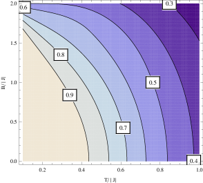
Figure 1: (Color online) Temperature-field phase diagram (left) and level lines (right) for the one-way deficit of the model under question with $J=\pm 1$ and $J_{z}=-1$. The fraction $\Delta_{\vartheta}$ is located between the solid lines 0 and 1 on the phase diagram; dotted line corresponds to the condition $\Delta_{0}=\Delta_{\pi/2}$ and does not here serve as the boundary. The strait line $B/|J|=1.4$ is a path for probing the shape of $\tilde{S}(\theta)$. Two pluses ($+$) on the boundaries 0 an 1 mark the points for characterizing the size of $\Delta_{\vartheta}$-region

The lines 0 and 1 are the 0- and $\pi/2$-boundaries corresponding to the solutions of Eqs. (29) and (30), respectively. The dotted line results from Eq. (28). Solution of Eq. (33) reproduces the solution of Eq. (29). These three lines tend to $T/|J|=0.91758$ when $B/|J|\to 0$ (see Fig. 1, on the left).

To identify different regions on the plane $(T,B)$ we will study the shapes of post-measurement entropy function $\tilde{S}(\theta)$ in various points of the plane. Let us take, for example, a straight line $B/|J|=1.4$ (see Fig. 1, left). Evolution of $\tilde{S}(\theta)$ by moving along this path is shown in Fig. 2.

Figure 2: Post-measurement entropy $\tilde{S}$ vs $\theta$ by $J=-1$, $J_{z}=-1$, $B=1.4$ and $T=1$ (a), 0.742967 (b), 0.72 (c), 0.684237 (d), 0.6275 (e), 0.4 (f)

When the argument $T$ is large enough the curve $\tilde{S}(\theta)$ exhibits a monotonically increasing shape as shown in Fig. 2 (a). Here a position of minimum lies at $\theta=0$ and does not depend on $T$ (stationary optimal measurement angle). This means that the region $\Delta_{0}$ is here. With decreasing $T$ the minimum of the post-measurement entropy at the point $\theta=0$ becomes broader, see Fig. 2 (b). Further decreasing the temperature bears an interior minimum [see Fig. 2 (c)] position of which depends now on $T$ what tells us that we have entered into the region $\Delta_{\vartheta}$ with the variable optimal measurement angle $\vartheta$. At the temperature $T=0.684237$ the path reaches the dotted line, where $\tilde{S}_{0}=\tilde{S}_{\pi/2}$ as clear seen in Fig. 2 (d). Then the interior minimum merges with the minimum at the endpoint $\theta=\pi/2$; this situation is shown in Fig. 2 (e). After this the region $\Delta_{\pi/2}$ with the constant optimal measurement angle $\theta=\pi/2$ takes place up to $T=0$. So, we have classified all subregions and hence obtain the phase diagram by $J_{z}/|J|=-1$.

It is interesting to estimate the characteristic width of the region with the variable optimal measurement angle. For this purpose we chose two points on the boundaries 0 and $\pi/2$ marked be symbols “plus” $(+)$ that have coordinates $(0.5444,1.8323)$ and $(0.4765,1.6164)$, see the left Figure 1. To find the width, one may use the fidelity $F$ which is related to the Bures distance $d_{B}$ by the equation $d_{B}=[2(1-\sqrt{F})]^{1/2}$. Since the density matrices $\rho_{AB}$ by different values of $a$, $b$, $d$ and $v$ commute, the fidelity is given as

$$F=\biggl{(}\sum_{j=1}^{4}\sqrt{\lambda_{j}^{(1)}\lambda_{j}^{(2)}}\biggr{)}^{\!\!2}.$$ (34)

Here $\lambda_{j}^{(1,2)}$ are the eigenvalues (9) for the two points taken on the plane $(T,B)$. Using Eq. (34) we get $F=0.985645$ ($\approx 98.6\%)$ between the above points. One may conclude from here that the region with the variable optimal measurement angle is broad enough and can be detected on an experiment (see in this connection MGY19 ).

The graph on the right side of Fig. 1 shows the distribution of one-way quantum work deficit values together with the level lines. The maximum value $\rm\Delta=1$ is achieved at the point $(0,0)$ and then, how it is clear seen from this figure, the quantum correlation asymptotically tends to zero when $T$ and $B$ increase.

3.2 Bifurcations and catastrophes at the boundaries

In this subsection, we will make a small digression and discuss in more detail the mechanism of the appearance and disappearance of interior extrema in the function $\tilde{S}(\theta)$.

To this end, let us look at the behavior of this function from the previous example ($J_{z}/|J|=-1$ and $B/|J|=1.4$) but in a wider window, namely $\theta\in[-\pi/2,\pi/2]$. Graphs of $\tilde{S}(\theta)$ at and near the 0-boundary are shown in Fig. 3.

Figure 3: Post-measurement entropy $\tilde{S}$ vs $\theta$ in the window $[-\pi/2,\pi/2]$ for the model by $J_{z}/|J|=-1$, $B/|J|=1.4$, and $T=T_{c}=0.742967$ (left) and $T=0.72$ (right). The bifurcation of the minimum at $\theta=0$ is clear visible: the behavior of function like $y\propto x^{4}$ (left) changes to $y\propto x^{4}-\epsilon x^{2}$ (right)

When the temperature is large enough the optimal measurement angle is a constant equal to zero and the minimized post-measurement entropy is described by the branch $\tilde{S}_{0}(T)$. Near the minimum $\theta=0$, the function $\tilde{S}(\theta)\sim\theta^{2}$. As the temperature $T\to T_{c}=0.742967$, the minimum broadens and at the point $T=T_{c}$ the function becomes like $\tilde{S}(\theta)\sim\theta^{4}$ (Fig. 3, left). However, with an arbitrary small further decrease in $T$ a “catastrophe” occurs: the local minimum at $\theta=0$ suddenly splits (bifurcates) into two ones (see Fig. 3, right), and the minimized post-measurement entropy, Eq. (26), changes (jumps) from $\tilde{S}_{0}(T)$ to the another branch $\tilde{S}_{\vartheta}(T)$.

The above picture is quantitatively described as follows. The function $\tilde{S}(\theta)$ is even and its expansion in a Tailor series at $\theta=0$ has the form

$$\tilde{S}(\theta;T,B)=\tilde{S}_{0}(T,B)+\frac{1}{2!}\tilde{S}^{\prime\prime}_{0}(T,B)\!\cdot\!\theta^{2}+\frac{1}{4!}\tilde{S}^{iv}_{0}(T,B)\!\cdot\!\theta^{4}+\ldots,$$ (35)

where $\tilde{S}_{0}(T,B)$ and $\tilde{S}^{\prime\prime}_{0}(T,B)$ are given by Eqs. (21) and (31), respectively. This series is similar to the Landau expansion of the thermodynamic potential (Gibbs free energy) in his theory of second order phase transitions LL_StPh . In our problem, $\tilde{S}(\theta)$ plays a role of the thermodynamic potential and the optimal measurement angle $\vartheta$ is an analogue of the order parameter in Landau’s theory. The vanishing of the coefficient at the quadratic term corresponds to the phase transition point.

Various sudden changes in behavior of a system as the variables that control it are changed continuously are studied and classified in the catastrophe theory A92 . Regarding our problem, it is useful to analyze the behavior of the function

$$f(\theta)=-t\theta^{2}+\theta^{4}.$$ (36)

For $\theta>0$, this function is either monotonically increasing (when the parameter $t\leq 0$) or unimodal (has one minimum), when $t>0$. In the latter case, the minimum is located at $\vartheta=\sqrt{t/2}$ and its depth equals $h=t^{2}/4$. Hence, the distance to this minimum increases with the speed $\dot{\vartheta}=1/(2\sqrt{2t})$, and the depth of the minimum grows with the speed $\dot{h}=t/2$. Thus, at the moment of birth $(t=0)$, the position of the minimum moves with infinite speed, whereas the depth of the minimum increases extremely slowly - with zero speed. The former is favorable to numerical search the interior minimum but the latter, on the contrary, makes the task difficult. Therefore, for finding the 0-boundary, it is better to use Eq. (29) than Eq. (33). Notice, the expansion of the quantity $t(T)$ at the point $T=T_{c}$ up to the first nonzero term is equal to $t=\alpha_{0}(T-T_{c})$.

Return again to the discussion of example from the previous subsection. When moving along the path $B/|J|=1.4$, the interior minimum reaches the $\pi/2$-boundary at the temperature $T=0.6275$ (see Fig. 1). Here the inner minimum merges with the minimum at the bound $\theta=\pi/2$ as shown in Fig. 2 (e). With further decreasing the temperature, the optimal measurement angle stays $\pi/2$ up to zero absolute temperature. So, one may conclude that, if the conditional or post-measurement entropy function is unimodal, then its local extremum can appear inside the open interval $(0,\pi/2)$ or, v.v., disappear in it only if the extremum enters or leaves trough one of two boundaries: at 0 or $\pi/2$. It was the observation that allowed in Refs. Y14 ; Y14a ; Y15 to propose the boundary equations, based on the second derivatives, for the regions with the variable optimal measurement angle.

Later, however, the bimodal behavior has been discovered in some cases for the one-way quantum work deficit Y18 . In the next subsection, we will meet such situations. To describe mathematically the bimodal behavior one should to expand the function under optimization up to sixth order terms:

$$f(\theta)=\alpha_{1}\theta^{2}+\alpha_{2}\theta^{4}+\theta^{6}.$$ (37)

For $\theta>0$, this function can have two local extrema: one minimum and one maximum. Under some conditions, the additional minimum can drop lower that the minimum at $\theta=0$. Then a new phenomenon arises, namely, the optimal measurement angle discontinuously changes/jumps from zero to the angle corresponding to the inner minimum (see Y18 ; Y19 and the next subsection). In the context of Landau’s theory, similar finite jumps of the order parameter corresponds the first order phase transitions.

This concludes the digression and we move on to discussing the types of phase diagrams again.

3.3 The case $J_{z}<-|J|$

Consider now the case when the coupling constant $J_{z}$ is negative and dominates in magnitude. This corresponds to the antiferromagnetic Ising-like systems. Let, for definiteness, J be equal to $-1$ and $J_{z}=-1.5$. In this case, the energy spectrum, Eq. (2), consists of two singlets and one doublet that is split into two levels by an external magnetic field as shown in Fig. 4.

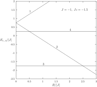
Figure 4: Splitting scheme of energy levels for the model with $J=-1$ and $J_{z}=-1.5$. Lines $1-4$ correspond to the energies $E_{1}-E_{4}$, respectively

The energy level $E_{2}=-J_{z}/2-B$ crosses the singlet levels $E_{3}=J_{z}/2+J$ and $E_{4}=J_{z}/2-J$ at $B/|J|=2.5$ and $0.5$, respectively.

Formal solution of the boundary equations (28) - (30) and (33) leads to the curves shown on the left in Fig. 5 by the dotted, 0, 1, and $0^{\prime}$ lines, respectively.

Figure 5: On the left, the curves corresponding to the solutions of all boundary equations and, on the right, the phase diagram of the one-way deficit for the system with $|J|=1$ and $J_{z}=-1.5$. Black circle ($\bullet$) is the triple point. Straight lines $B/|J|=1.9$ and $B/|J|=1.2$ are the paths along which the shapes of $\tilde{S}(\theta)$ are studied (see Figs. 6 and 7)

The dotted curve, a candidate on the boundary $\Delta_{0}=\Delta_{\pi/2}$, and the curves 1 and $0^{\prime}$ intersect at the point $(0.6454108,1.6851637)$ marked by the black circle.

In order to identify each area of the plane $(T,B)$ we will again study the shapes of the post-measurement entropy function $\tilde{S}(\theta)$ in all subregions. Let us examine, for example, the shapes moving along the path $B/|J|=1.9$. Evolution of the $\tilde{S}(\theta)$ curve is depicted in Fig. 6 (a)-(f).

Figure 6: Post-measurement entropy $\tilde{S}$ vs $\theta$ by $J=-1$, $J_{z}=-1.5$, $B=1.9$ and $T=0.7$ (a), 0.64 (b), 0.637 (c), 0.63329 (d), 0.628 (e), 0.62378 (f), 0.61471 (g), 0.59669 (h), and 0.5 (i)

When the temperature is high enough, the curve $\tilde{S}(\theta)$ has the monotonically increasing behavior as shown in Fig. 6 (a) by $T=0.7$. Its minimum is located at $\theta=0$ and hence this is the region $\Delta_{0}$ (see the right part of Fig. 5).

However, as the system cools, the shape of the curve begins to deform and an inflection point with the horizontal tangent appears at $T=0.637$ [see Fig. 6 (b) and (c)].

With further decreasing the temperature, the dependence $\tilde{S}(\theta)$ becomes bimodal in the open interval $(0,\pi/2)$. At $T=0.63329$ we arrive at the $0^{\prime}$-boundary (see the right part in Fig. 5) where the value of minimum reaches the value of $\tilde{S}(\theta)$ at $\theta=0$. This moment is fixed in Fig. 6 (d). The optimal measurement angle suddenly jumps from zero to the interior minimum angle $\vartheta$ for any arbitrary small decreasing the temperature.

The jumps $\Delta\vartheta$ depend on the strength of magnetic field. The values of jumps by different $B/|J|$ are collected in Table 1.

Table 1: Jumps of optimal measured angles, $\Delta\vartheta$, on the boundary $0^{\prime}$ for the model with $J=-1$ and $J_{z}/|J|=-1.5$

$B/|J|$	$T/|J|$	$\Delta\vartheta$
$1.6851637$	$0.6454108$	$1.570782\approx 90^{\circ}$
$1.7$	$0.64533$	$1.30773\approx 74.9^{\circ}$
$1.8$	$0.64193$	$0.86605\approx 49.6^{\circ}$
$1.9$	$0.63329$	$0.64026\approx 36.7^{\circ}$
$2.0$	$0.61883$	$0.48104\approx 27.6^{\circ}$

It is seen from the table that the jump is largest (equal to $\pi/2$) at the triple point (marked in figures by black circles) and gradually disappears with increasing $B$.

Let us go back to the path $B/|J|=1.9$ and Fig. 6. After crossing border $0^{\prime}$, the system enters region $\Delta_{\vartheta}$ shown on the right in Fig. 5. Here the interior maximum moves to the endpoint $\theta=0$ while the interior minimum, on the contrary, goes to the other endpoint, namely, $\theta=\pi/2$. This situation is shown in Fig. 6 (e).

The path intersects the dotted line at $T=0.62378$, where the values of post-measurement entropies at both endpoints coincide, see Fig. 6 (f).

When the temperature reaches the value of $T=0.61471$, the inverse process to the bifurcation is happened: the interior maximum merges with the maximum at the endpoint $\theta=0$ and the function $\tilde{S}(\theta)$ again becomes unimodal in the interval $(0,\pi/2)$. See Fig. 6 (g).

Then, at $T=0.59669$, the interior minimum reaches the endpoint $\theta=\pi/2$ as shown in Fig. 6 (h) and the optimal measurement angle continuously changes to the stationary optimal value of $\pi/2$, see Fig. 6 (i). This corresponds to the $\Delta_{\pi/2}$-region presented in the phase diagram of one-way deficit (Fig. 5, right).

Let us study now another a matter of principle case, namely, the case when the horizontal path goes below the triple point. Take for instance the path $B/|J|=1.2$ (see Fig. 5, left). The evolution of shape of the curves $\tilde{S}(\theta)$ by moving along this path is depicted in Fig. 7.

Figure 7: Post-measurement entropy $\tilde{S}$ vs $\theta$ by $J=-1$, $J_{z}=-1.5$, $B=1.2$ and $T=0.7$ (a), 0.54836 (b), 0.35 (c)

When the temperature is high enough the curve $\tilde{S}(\theta)$ exhibits a monotonically increasing behavior that is illustrated in Fig. 7 (a). The optimal measurement angle is zero and therefore this is the region $\Delta_{0}$. Moving into the lower temperatures the path reaches the line 1 ($\pi/2$-boundary). At the intersection point, a bifurcation of maximum at the endpoint $\theta=\pi/2$ occurs and the interior maximum is born. However, the measurement angle that minimized $\tilde{S}(\theta)$ stays zero. When the dotted line is reached, the values of $\tilde{S}(\theta)$ at both endpoints become equal. This moment of equilibrium is fixed in Fig. 7 (b). With an arbitrary small decrease in temperature, the optimal measurement angle discontinuously changes from zero to $\pi/2$, and the region $\Delta_{\pi/2}$ begins. Then, at the line 0, the interior maximum annihilates at the endpoint $\theta=0$ via the inverse bifurcation mechanism. After that, the curve $\tilde{S}(\theta)$ has a monotonically decreasing shape as drawn in Fig. 7 (c). This corresponds to the region $\Delta_{\pi/2}$ up to $T=0$, see Fig. 5. So, the line obeying the equation (28) serves here as the boundary between the regions $\Delta_{0}$ and $\Delta_{\pi/2}$. This boundary is shown on the right part of Fig. 5 by the solid line and marked by the symbol 2. So, we complete the construction of phase diagram shown in Fig. 5 on the right.

Auxiliary constructions and phase diagrams with an even more pronounced Ising’s character of interactions are presented in Figs. 8 and 9.

Figure 8: Lines corresponding to formal solution of the boundary equations (left) and the phase diagram (right) for the system with $J=\pm 0.5$ and $J_{z}=-1$. The triple point (black circle) has coordinates $(0.313637,1.12742)$. Normalization on $|J_{z}|$ is used here

Figure 9: Lines corresponding to formal solution of the boundary equations (left) and the phase diagram (right) for the system with $J=\pm 0.2$ and $J_{z}=-1$. Coordinates of the triple point are $(0.1244107,1.055204)$. Here normalization is done on $|J_{z}|$

Here the quantity $J_{z}$ is kept constant and the interaction $J$, on the contrary, decreases. This better reflects the situation in the model. It is seen from the phase diagrams that the area of the phases $\Delta_{\pi/2}$ and $\Delta_{\vartheta}$ goes to zero and vanishes at all in the limit $|J|\to 0$. As a result, the entire plane $(T,B)$ is occupied by a single phase $\Delta_{0}$.

This completes a construction of the phase diagrams for the parameters $J$ and $J_{z}$ provided $J_{z}<-|J|$.

3.4 The case $-|J|<J_{z}\leq 0$

When $J_{z}/|J|\geq-1$, the boundary $0^{\prime}$ is absent or, more correctly, it coincides the 0-boundary. In other words, there are no jumps of optimal measurement angle $\vartheta$ on finite steps $\Delta\vartheta>0$, but less than $\pi/2$; the angle $\vartheta$ in the region $\Delta_{\vartheta}$ varies continuously from zero to $\pi/2$. Typical phase diagrams under question are shown in Fig. 10.

Figure 10: Phase diagram for $|J|=1$ and $J_{z}=-0.9$ (left) and $-0.5$ (right). Region $\Delta_{\vartheta}$ lies between the boundaries 0 and 1. Dotted line corresponds to the condition $\Delta_{0}=\Delta_{\pi/2}$

The directionality of changes in curves 0 and 1 is clearly seen when the longitudinal interaction $J_{z}$ tends to zero.

In the limit $J_{z}\to 0$, the model is transformed into the XX one. In accord with Eqs. (2.1), (29) and (31), the equation for the 0-boundary by $J_{z}=0$ is given as

$$\sinh^{2}\bigg{(}\frac{J}{T}\bigg{)}\Bigg{[}\frac{\ln[\exp(B/T)/\cosh(J/T)]}{\exp(B/T)-\cosh(J/T)}+\frac{\ln[\cosh(J/T)/\exp(-B/T)]}{\cosh(J/T)-\exp(-B/T)}\Bigg{]}$$

$$=\frac{2B}{T}\sinh\bigg{(}\frac{B}{T}\bigg{)}-4\bigg{[}\cosh\bigg{(}\frac{B}{T}\bigg{)}-\cosh\bigg{(}\frac{J}{T}\bigg{)}\bigg{]}\ln\!\bigg{[}\cosh\bigg{(}\frac{J}{T}\bigg{)}\bigg{]}.$$ (38)

This transcendental equation can be solved analytically. Indeed, it is easy to check that the substitution $B=|J|$ satisfies the equation (3.4). Thus, the 0-boundary is here the strait line $B/|J|=1$ parallel to the abscissa axis. The phase diagram in this limit is depicted in Fig. 11.

Figure 11: Phase diagram for the XX dimer $(J_{z}=0)$. Region $\Delta_{\vartheta}$ is located between the lines 0 and 1. Dotted line corresponds to the condition $\Delta_{0}=\Delta_{\pi/2}$

The second boundary, line 1, is a curve containing the interior local minimum with coordinates $(0.404,0.7716)$. The fidelity between quantum states at this point and the nearest one on the 0-boundary, i.e., at point $(0.404,1)$ equals $F=0.97994$ ($\approx 97.99\%$). This value characterizes the width of $\Delta_{\vartheta}$-region. The region near this minimum is broad enough and therefore one can try to reach it in an experiment.

3.5 The case $0<J_{z}\leq|J|$

Figure 12: Phase diagram for $|J|=1$ and $J_{z}=0.5$ (left) and $0.9$ (right). The region $\Delta_{\vartheta}$ lies between the boundaries 0 and 1. Dotted line corresponds to the condition $\Delta_{0}=\Delta_{\pi/2}$

So when $J_{z}=0$, the phase diagram looks as shown in Fig. 11. Let us continue to increase the value of interaction $J_{z}$. Phase diagrams at $J_{z}/|J|=0.5$ and 0.9 are presented in Fig. 12. One can see that the 0- and $\pi/2$-boundaries drop down to the abscissa axis when the quantity $J_{z}/|J|$ tends to unity. In the limit $Jz/|J|\to 1$, the regions $\Delta_{\pi/2}$ and $\Delta_{\vartheta}$ disappear completely and the phase $\Delta_{0}$ occupies the entire area of plane $(T,B)$.

3.6 The case $J_{z}>|J|$

When the coupling $J_{z}$ is grater than $|J|$, the system belongs to the Ising-like ferromagnetic type. The $z$-component of the spin interaction dominates. As the analysis shows, the phase diagram consists here of one fraction $\Delta_{0}$ at any temperatures $T$ and strengths of the field $B$.

It is interesting to compare this result with the behavior of quantum discord. In contrast to the one-way deficit, the quantum discord exhibits different behavior for the same choice of coupling constants. Indeed, as shown in Fig. 4 of Ref. Y14 for $J=1$ and $J_{z}=1.02$, the phase diagram of the quantum discord consists of three regions corresponding to the optimal measurement angles zero, $\pi/2$, and an angle in the intermediate interval between zero and $\pi/2$ (the region with the interior optimal measurement angle).

Such a discrepancy indicates the imperfectness of existing concepts of quantum correlations. We unfortunately have to admit that we do not know for sure what measure of quantum correlation is true. Only further progress in the field of theory and practice of quantum correlations will help resolve the contradictions existing today.

4 Summary and conclusions

In this paper, we have performed analysis and constructed the temperature-field phase diagrams of one-way quantum work deficit for the two-qubit XXZ model in a uniform magnetic field. The set of figures presented in Sect. 3 (first of all, Figs. 1, 5, 10, 11, and 12) gives a complete picture of the qualitatively different types of $(T,B)$-diagrams in the entire range of values for the parameter $J_{z}$, i.e., in the three-dimensional space $(T,B,J_{z})$.

We have also described the special properties of post-measurement entropy that are important in planning and performing an experiment. The diagrams allow to predict where the quantum correlation will experience the different features due to jumps of optimal measurement angle. Thus, the presented diagrams can serve as a kind of routings useful for experimenters in their work.

In addition, we have established a connection between the cause of the appearance of boundaries separated different fractures of the quantum correlation and Landau’s approach to the problem of phase transitions as well as the mathematical theory of catastrophes.

Further development of the presented results is associated with the consideration of more general spin systems. However, this will require consideration of multidimensional spaces, which will certainly make the problem much more difficult. One can rely a hope for virtual reality methods which are developed now very rapidly.

Acknowledgments I am grateful to A. I. Zenchuk for his help. This work was performed as a part of the state task, State Registration No. 0089-2019-0002.

References

- (1) Modi, K., Brodutch, A., Cable, H., Paterek, T., Vedral, V.: The classical-quantum boundary for correlations: discord and related measures. Rev. Mod. Phys. 84, 1655 (2012)
- (2) Streltsov, A.: Quantum correlations beyond entanglement and their role in quantum information theory. Springer, Berlin (2015)
- (3) Adesso, G., Bromley, T.R., Cianciaruso, M.: Measures and applications of quantum correlations. J. Phys. A: Math. Theor. 49, 473001 (2016)
- (4) Lectures on general quantum correlations and their applications. Eds: Fanchini, F.F., Soares-Pinto, D.O., Adesso, G. Springer, Berlin (2017)
- (5) Bera, A., Das, T., Sadhukhan, D., Roy, S.S., Sen(De), A., Sen, U.: Quantum discord and its allies: a review of recent progress. Rep. Prog. Phys. 81, 024001 (2018)
- (6) Feynman, R.P., Leighton, R.B., Sands, M.: The Feynman lectures on physics. Addison-Wesley, Reading, Mass. (1964, second printing). - Sect. 38-6
- (7) Heisenberg, W.: ber quantentheoretische Umdeutung kinematischer und mechanischer Beziehungen. Zs. Phys. 33, 879 (1925)
- (8) Wolff, J.: Heisenberg’s observability principle. In: Studies in history and philosophy of science. Part B. Studies in history and philosophy of modern physics 45, 19 (2014)
- (9) Zurek, W.H.: Einselection and decoherence from an information theory perspective. Ann. Phys. (Leipzig) 9, 855 (2000)
- (10) Ollivier, H., Zurek, W.H.: Quantum discord: a measure of the quantumness of correlations. Phys. Rev. Lett. 88, 017901 (2002)
- (11) Henderson, L., Vedral, V.: Classical, quantum and total correlations. J. Phys. A: Math. Gen. 34, 6899 (2001)
- (12) Vedral, V.: Foundations of quantum discord. In: Lectures on general quantum correlations and their applications. Eds: Fanchini, F.F., Soares-Pinto, D.O., Adesso, G. Springer, Berlin (2017)
- (13) Lindblad, G.: Entropy, information and quantum measurements. Commun. Math. Phys. 33, 305 (1973)
- (14) Oppenheim, J., Horodecki, M., Horodecki, P., Horodecki, R.: Thermodynamical approach to quantifying quantum correlations. Phys. Rev. Lett. 89, 180402 (2002)
- (15) Horodecki, M., Horodecki, K., Horodecki, P., Horodecki, R., Oppenheim, J., Sen(De), A., Sen, U.: Local information as a resource in distributed quantum systems. Phys. Rev. Lett. 90, 100402 (2003)
- (16) Horodecki, M., Horodecki, P., Horodecki, R., Oppenheim, J., Sen(De), A., Sen, U., Synak-Radtke, B.: Local versus nonlocal information in quantum-information theory: Formalism and phenomena. Phys. Rev. A 71, 062307 (2005)
- (17) Ye, B.-L., Fei, S.-M.: A note on one-way quantum deficit and quantum discord. Quantum Inf. Process. 15, 279 (2016)
- (18) Feynman, R.: The character of physical law. MIT, Cambridge, Mass. (1985, twelfth printing). - Sect. 7 Seeking new laws, p. 164
- (19) Lu, X.-M., Xi, Z., Sun, Z., Wang, X.: Geometric mesure of quantum discord under decoherence. Quantum Inf. Comput. 10, 0994 (2010)
- (20) Ciliberti, L., Rossignoli, R., Canosa, N.: Quantum discord in finite chains. Phys. Rev. A 82, 042316 (2010)
- (21) Vinjanampathy, S., Rau, A.R.P.: Quantum discord for qubit-qudit systems. J. Phys. A: Math. Theor. 45, 095303 (2012)
- (22) Ye, B.-L., Wang, Y.-K., Fei, S.-M.: One-way quantum deficit and decoherence for two-qubit states. Int. J. Theor. Phys. 55, 2237 (2016)
- (23) Yurischev, M.A.: Bimodal behavior of post-measured entropy and one-way quantum deficit for two-qubit X states. Quantum Inf. Process. 17:6 (2018)
- (24) Yurischev, M.A.: Phase diagram for the one-way quantum deficit of two-qubit X states. Quantum Inf. Process. 18:124 (2019)
- (25) Lu, X.-M., Ma, J., Xi, Z., Wang, X.: Optimal measurements to access classical correlations of two-qubit states. Phys. Rev. A 83, 012327 (2011)
- (26) Chen, Q., Zhang, C., Yu, S., Yi, X.X., Oh, C.H.: Quantum discord of two-qubit states. Phys. Rev. A 84, 042313 (2011)
- (27) Huang, Y.: Quantum discord for two-qubit states: analytical formula with very small worst-case error. Phys. Rev. A 88, 014302 (2013)
- (28) Yurischev, M.A.:, Quantum discord for general X and CS states: a piecewise-analytical-numerical formula, arXiv:1404.5735v1 [quant-ph]
- (29) Yurishchev, M.A.:, NMR dynamics of quantum discord for spin-carrying gas molecules in a closed nanopore. J. Exp. Theor. Phys. 119, 828 (2014); arXiv:1503.03316v1 [quant-ph]
- (30) Yurischev, M.A.: On the quantum discord of general states. Quantum Inf. Process. 14, 3399 (2015)
- (31) Yurischev, M.A.: Extremal properties of conditional entropy and quantum discord for XXZ, symmetric quantum states. Quantum Inf. Process. 16:249 (2017)
- (32) Canosa, N., Ciliberti, L., Rossignoli, R.: Quantum discord and information deficit in spin chains. Entropy 17, 1634 (2015) (Special issue: Quantum computation and information: Multi-particle aspects)
- (33) Klein, O.: Zur quantenmechanischen Begrndung des zweiten Hauptsatzes der Wrmelehre. Zs. Phys. 72, 767 (1931)
- (34) Nielsen, M.A., Chuang, I.L.: Quantum computation and quantum information. 10th anniversary edition. Cambridge University Press, Cambridge (2010), Sect. 11.3.3
- (35) Fain, V.M.: Quantum radiophysics. Vol. 1. Photons and nonlinear media. Second edition. Sovetskoe Radio, Moscow (1972) [in Russian]
- (36) Dirac, P.A.M.: The principles of quantum mechanics. Fourth edition. Clarendon, Oxford (1958), Sect. II.10
- (37) James, D.F.V., Kwiat, P.G., Munro, W.J., White, A.G.: Measurement of qubits. Phys. Rev. A 64, 052312 (2001)
- (38) Yurischev, M.A.: Jumps of optimal measurement angle and fractures on the curves of quantum correlation functions. Proc. of SPIE 11022, 1102221 (2019)
- (39) Moreva, E.V., Gramegna, M., Yurischev, M.A.: On the possibility to detect quantum correlation regions with the variable optimal measurement angle. Eur. Phys. J. D 73:68 (2019), topical issue “Quantum correlations”
- (40) Landau, L.D., Lifshitz, E.M.: Statistical physics. Part 1. Fizmatlit, Moscow (2005) [in Russian], Pergamon, Oxford (1980) [in English]
- (41) Arnold, V.I.: Catastrophe theory. Springer, Berlin (1992), Sect. 10