The angular resolution of GRAPES-3 EAS array after correction for the shower front curvature

Abstract

The angular resolution of an extensive air shower (EAS) array plays a critical role in determining its sensitivity for the detection of point $\gamma$-ray sources in the multi-TeV energy range. The GRAPES-3 an EAS array located at Ooty in India (11.4^∘N, 76.7^∘E, 2200 m altitude) is designed to study $\gamma$-rays in the TeV-PeV energy range. It comprises of a dense array of 400 plastic scintillators deployed over an area of 25000 m² and a large area (560 m²) muon telescope. A new statistical method allowed real time determination of the propagation delay of each detector in the GRAPES-3 array. The shape of shower front is known to be curved and here the details of a new method developed for accurate measurement of the shower front curvature is presented. These two developments have led to a sizable improvement in the angular resolution of GRAPES-3 array. It is shown that the curvature depends on the size and age of an EAS. By employing two different techniques, namely, the odd-even and the left-right methods, independent estimates of the angular resolution are obtained. The odd-even method estimates the best achievable resolution of the array. For obtaining the angular resolution, the left-right method is used after implementing the size and age dependent curvature corrections. A comparison of the angular resolution as a function of EAS energy by these two methods shows them be virtually indistinguishable. The angular resolution of GRAPES-3 array is 47^′ for energies E$>$5 TeV and improves to 17^′ at E$>$100 TeV and finally approaching 10^′ at E$>$500 TeV.

1 Introduction

The origin of primary cosmic rays (PCRs) is a fundamental problem of high-energy astrophysics which has remained unresolved even after their discovery by Hess more than a century ago. The charged nature of PCRs causes their path to be continuously modified due to passage through space permeated by randomly oriented magnetic fields. Consequently, their directions get completely randomised that bear no relation to the sources of their origin. On the other hand, the small flux of primary $\gamma$-rays, produced along with the charged PCRs travel in a straight line from the sources of their origin allowing detection of the sources of PCRs [1]. Past two decades have witnessed phenomenal progress in the field of $\gamma$-ray astronomy in the MeV-GeV energy range and a very large number of sources have been discovered by space-borne telescopes. However, in the GeV-TeV energy range the $\gamma$-ray flux is too low to be detected by the present modest area telescopes flown on the satellites. The ground-based imaging atmospheric Cherenkov telescopes (IACTs) which detect the faint Cherenkov light emitted by the electrons in an extensive air shower (EAS) are ideally suited for the detection of sub-TeV $\gamma$-rays [2]. The EAS arrays enjoy a unique advantage due to the following two factors, (i) a very large field of view $>$3 sr compared to $<$0.03 sr for the IACTs, (ii) a duty cycle of $\sim$100% compared to $<$10% for the IACTs. However, the EAS arrays generally suffer from poorer angular resolution ($>$1^∘ at 100 TeV) as compared to the IACTs ($<$0.1^∘). The flux of $\gamma$-rays decreases rapidly with energy and becomes extremely small at multi-TeV energies thus, it becomes extremely difficult to detect it in an overwhelming background of isotropic PCRs. Since the signal to noise ratio for a telescope scales inversely with its angular resolution thus, it becomes critically important to achieve as small an angular resolution as possible which is precisely the strategy devised for the GRAPES-3 EAS array.

So far 100 TeV $\gamma$-rays have been detected from only a handful of galactic sources including a supernova remnant and a pulsar which might be sites of particle acceleration to PeV energies within our galaxy [3, 4]. Most of the sub-TeV $\gamma$-ray sources seem to be leptonic in origin where $\gamma$-rays are produced via inverse Compton scattering of synchrotron photons produced by TeV electrons. In general, the inverse Compton scattering is strongly suppressed by the Klein-Nishina effect at high energies and therefore, above 100 TeV $\gamma$-rays are expected to be mostly of hadronic origin. These $\gamma$-rays are produced during the decay of neutral pions generated in the interactions PeV protons with the ambient matter. Therefore, the observation of multi-TeV $\gamma$-ray sources is essential for addressing the problem of origin of PCRs [1].

As discussed above, EAS arrays enjoy an advantage over the IACTs in terms of longer observation time and a far greater sky coverage and are therefore ideally suited for monitoring a large number of sources and to search for new ones. But these arrays suffer from poorer angular resolution thus making them less competitive than the IACTs for the discovery of new sources. Typically, the IACTs have an excellent angular resolution of 5–8^′ in the sub-TeV energy region [5, 6, 7]. In EAS arrays the shower direction is obtained from the information on the relative arrival time of particles in the triggered detectors. These particles are primarily electrons and muons which exhibit considerable fluctuations due to various processes such as multiple scattering and transverse momentum imparted during the shower development. Therefore, the shower front acquires a disc-like structure, about 1-2 m thick near the central core of the shower which increases with increasing distance from the core. The mean energy of particles decreases away the core due to delays caused by multiple scattering etc. Consequently, the shower front exhibits a curved profile away from the shower core [8]. A number of studies have shown the the presence of a curvature in the shower front [9, 10, 11, 12]. Extensive Monte Carlo simulation studies have also suggested the existence of shower front curvature [13, 14]. This curvature needs to be corrected for accurate measurement of the EAS direction and for that a precise measurement of the curvature becomes an essential prerequisite for improving the angular resolution of an EAS array. A discussion of the origin of shower front curvature and finite disc structure can be found in a monograph by Grieder [15]. The curved shower front is adequately described by a cone centred on the shower axis for distances up to 100–200 m [16, 17]. By implementing curvature correction an angular resolution of 1.1^∘ at 150 TeV was reported for the KGF EAS array [16].

The EAS arrays record showers of varying size (N_e) and age (s). While the size is proportional to energy of the PCR, the age characterizes the stage of the shower development. In recent past some attempts were made to study the relationship of the shower front curvature on shower size [16, 18, 19, 20]. However, the work presented here is possibly the first systematic investigation of the dependence of shower front curvature on both the shower size and age. In §2 after a very brief overview of the GRAPES-3 array, the methodology for measurement of the arrival times of EAS particles is presented. In §3, detailed investigation of the shower front curvature is presented. This is followed by §4 where the measurement of the angular resolution by two distinctly different techniques, namely, the odd-even and left-right methods are presented. Next, a comparative study of the GRAPES-3 angular resolution with other major arrays operating elsewhere in the world is presented §5. Finally the conclusions of this study are summarised in §6.

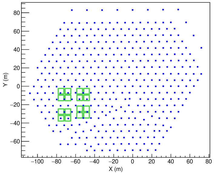
Figure 1: GRAPES-3 EAS array in Ooty, India (11.4^∘N, 76.7^∘E, 2200m a.s.l). Small filled squares represent scintillator detectors of 1 m² area each separated by 8 m and the 16 big squares represent muon modules of 35 m² area each.

2 Measurement of time of shower particle

The GRAPES-3 experiment is located at Ooty, India at an altitude of 2200 m (11.4^∘N, 76.7^∘E). The two major components of the array include (i) 400 plastic scintillator detectors (each 1 m²) spread over 25000 m² [21, 22] and a tracking muon detector of 560 m² area with a threshold of 1 GeV [23]. A schematic of the array is shown in Fig. 1. The scintillator array is triggered by EAS produced by the PCRs in the energy range 10¹²–10¹⁶ eV. Over 10⁹ EAS are recorded every year. A detailed description of the trigger and the data acquisition may be found elsewhere [21]. Since the scintillator detectors are unshielded they record particles that deposit a few MeV of energy which is mainly contributed by the electrons, positron, muons and $\gamma$-rays albeit with a rather small efficiency ($\sim$5%). Each scintillator detector is instrumented to measure both the density and the arrival time of detected particles relative to the trigger. This information is used to determine the energy and the incident direction of the PCR responsible for producing the EAS.

Since the arrival direction of an EAS is determined by using the relative arrival time of particles in the shower front by the triggered detectors in the array, precise measurement of arrival times is the key requirement for achieving a good angular resolution. In GRAPES-3, the time is measured by a 32 channel high performance time-to-digital converter (HPTDC) which was developed in-house from an application specific integrated circuit designed and developed by the Microelectronics group at CERN, Geneva for the LHC experiments [24].

The signal from each scintillator is detected by a photomultiplier tube (PMT) and transmitted through a 230 m long, low-loss, co-axial cable (5D2V) to the control room. Subsequently, the signals from each scintillator is amplified, discriminated and its arrival time relative to the EAS trigger is digitized by the HPTDC with a resolution of 195 ps. The HPTDCs utilize a quartz oscillator to measure time, and therefore provide an exceptional performance in terms of long-term stability and linearity especially compared to the commercial TDCs.

The time T_i measured by detector “i” consists of two parts, namely, T_Ei the variable part contributed by particles in the EAS, and second T_Zi the passive part contributed by the delay in PMT, co-axial cable, and signal processing electronics etc. which is also called TDCZero. Ideally, T_Zi should remain constant, however, as shown later that this is not the case. To achieve a good angular resolution, it is important to accurately measure both of these parts. Although the signal from each scintillator detector ‘i’ to the HPTDC is transmitted by equal length cables, however, T_Zi shows significant variation from detector to detector possibly due to the differences in the response time of each detector, which includes the transit time inside PMT, unequal propagation velocities in co-axial cables etc.

Traditionally, the T_Zi for each detector in the GRAPES-3 experiment was measured relative to a common detector called “muon paddle” which is placed below the detector and used to trigger on muons passing through the scintillator above. The arrival time and charge contained in the PMT pulse produced by through going muons is measured by HPTDC and a charge integrating ADC, respectively for a duration of one hour. The most probable value of the TDC distribution is defined as the T_Zi for detector ‘i’. By moving the muon paddle manually from one detector to the next, the T_Zi for every detector in the array is measured [21]. One complete cycle of measurements takes $\sim$40 d owing to the fact that only 8–10 detectors can be manually calibrated in a single day. However, it is observed that T_Zi varies significantly even on a short time scale of a day. This is subsequently shown to be dependent on the ambient temperature. Thus, it becomes essential to develop an alternative technique for measuring T_Zi on time scale shorter than a day. The GRAPES-3 array records $\sim$10⁵ EAS every hour and by taking advantage of this high statistics data, an effective technique has been developed to determine the T_Zi on hourly time-scale as explained below.

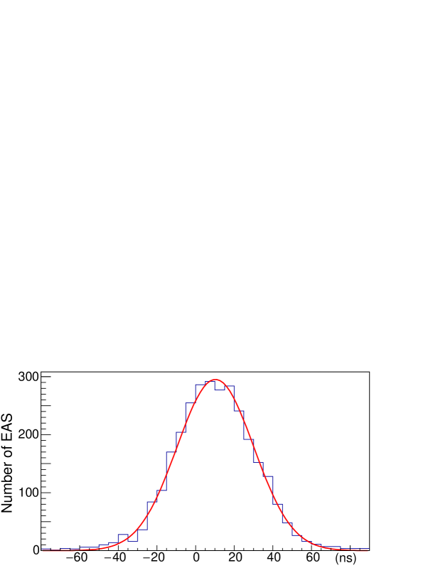
Figure 2: Distribution of arrival time difference of particles recorded by detector 1 and 9 for 1 h. Gaussian fit to data yields a peak at (10.3$\pm$0.4) ns and $\sigma$ of 19.9 ns.

The distribution of arrival time difference ($\Delta$t) of any two detectors (i,j) represents the distribution of projected angles of the EAS incident in the array. The peak of $\Delta$t distribution is a measure of the difference T_Zi-T_Zj. Fig. 2 shows the $\Delta$t distribution for detectors 9 and 24 (separated by 16 m) generated from one hour of EAS data. A Gaussian fit to this distribution yields a peak value (10.3$\pm$0.4) ns and a standard deviation $\sigma$=19.9 ns. The value of $\sigma$ is proportional to the detector separation. However, for accurate direction reconstruction T_Z needs to be measured for each detector relative to a single reference detector in the array. For detector further away from the reference detector, the EAS would be of increasingly larger size and number of such EAS would rapidly decline. In addition, the width $\sigma_{t}$ of the $\Delta$t distribution increases proportional to the distance of the detector and the reference detector. Therefore, estimating T_Z for distant detectors becomes rapidly inaccurate. For example, for a distance of 80 m $\sigma_{t}$=94 ns. Also the number of EAS reduces by more than a factor of two, thus, the error in T_Z increases to 2.4 ns which is eight times larger than for a distance of 16 m. Below, a novel technique called “random walk method” which addresses this problem by proving a robust, real-time and accurate estimate of the T_Z for every detector in the array relative to a common reference detector is described.

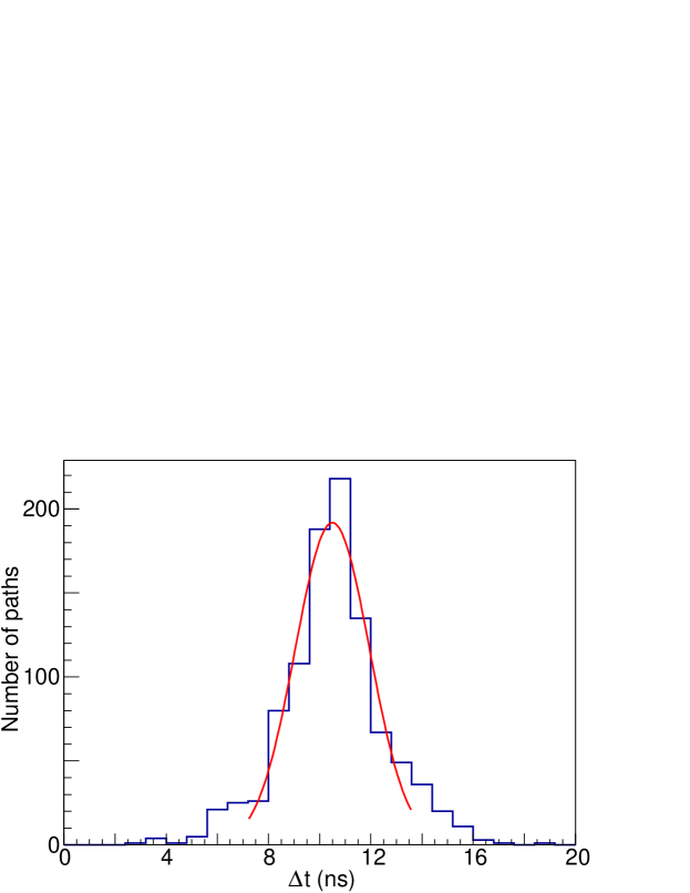
Figure 3: Distribution of TDCZero ‘T_Z’ for detector 24 relative to reference detector 9 based on 1000 random walk paths. The peak from a Gaussian fit occurs at (10.5$\pm$0.1) ns.

Here, the analysis of data collected during 2014 is presented. During 2014, detector 9 had exhibited a very stable performance and it had operated continuously without breakdown as well as displayed a stable gain. Therefore, detector 9 is selected as the reference detector. As a first step, the peak value $\tau_{jk}$ (k=1,12) of the $\Delta$t distribution of each detector ‘j’ in the array relative to its 12 neighbours is calculated. Here a pair of detectors separated by 16 m are termed “neighbours”. Next, starting from the reference detector 9 to any detector ‘i’ can be reached by a series of random steps to one of the 12 nearest neighbours by generating a random number with 12 discrete values which is equivalent to the rolling of a 12-sided dice. After the first random step, only 11 out of the 12 random steps is allowed to prevent the reverse step. This procedure is repeated until the reference detector is reached after N steps. However, if N exceeds 100, this random path is rejected and a new path is generated. Then the sum t_i=$\Sigma\tau_{jk}$ for N steps is calculated. A total of 1000 random paths are generated for the EAS data of each hour and a distribution of t_i is obtained as shown in Fig. 3 and the peak of this distribution provides a measure of T_Zi. A Gaussian fit to this distribution yields a value of (10.5$\pm$0.1) ns. The choice of limiting the random path to 100 steps and total number of paths to 1000 is based on the fact that increasing these values does not result in any improvement in the accuracy of measured T_Zi. However, when the detector performance is not stable the the distribution of t_i becomes broader and yet in most such cases the peak of the distribution is unaffected and hence the measured value of T_Zi stays unchanged.

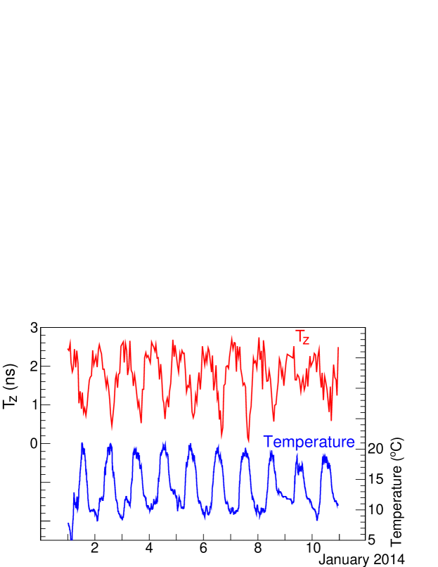
Figure 4: Hourly variation of, (i) T_Z for detector 24, (ii) temperature during 1–10 January 2014. An anti-correlation of T_Z and temperature is observed.

In Fig. 4 the hourly variation of T_Z for detector 24 and the ambient temperature outside is shown during 1–10 January 2014. The variation of T_Z is clearly anti-correlated with the temperature and an excursion as large as 2.5 ns in T_Z is observed in a single day which is significantly larger than the 0.195 ns resolution of the HPTDC used to record time. The co-axial cable used to transmit the PMT signal from detector 24 to the HPTDC located in the control room was replaced and was lying exposed. Thus, the variation of T_Z is caused by the temperature dependence of the dielectric constant of the insulator used in the co-axial cable. Because, the detectors whose signal cable are buried under the soil do not show such variation. However, the unique ability to measure hourly T_Z allows any variation in arrival time to be accurately measured and corrected.

3 Shower front curvature

A major challenge in improving the angular resolution of an EAS array depends on the ability to accurately measure the TDCZeros in real time and then the shape of the shower front. It is known that shower front does not have a plane shape and shows significant curvature [25]. Thus, the measurement of shower front curvature becomes an important tool for improving the angular resolution of an EAS array. But before measuring the curvature, approximate direction of the EAS can be obtained by fitting a plane to the observed arrival times of particles in each triggered detector after subtracting respective T_Z determined by the random walk method described in §2. The plane shower front is fitted by minimizing the quantity $\chi^{2}$

$$\rm\chi^{2}=\Sigma_{i}(lx_{i}+my_{i}+nz_{i}+c(t_{i}^{obs}-t_{0}))^{2}$$ (1)

Here, ${\rm l=sin\theta cos\phi}$, ${\rm m=sin\theta sin\phi}$ and ${\rm n=cos\theta}$ are the direction cosines of EAS axis and ${\theta}$, ${\phi}$ are the zenith and azimuthal angles, respectively. x_i, y_i, z_i are the detector locations and $\rm t_{i}^{obs}$ the arrival time measured by $\rm i^{th}$ detector. The shower front comprising of highly relativistic particles moves at nearly the speed of light and therefore, the velocity of light ‘c’ is used as the velocity of the shower front. Here, $\rm t_{0}$ is the reference time when the EAS hits a fictitious detector located at the EAS core.

To determine the shower front curvature, the core location of the EAS should be known. By fitting a lateral distribution function, namely, the Nishimura-Kamata-Greisen (NKG) to the observed particle densities by a maximum likelihood algorithm MINUIT, the core location (X_c, Y_c) and other EAS parameters such as EAS size ‘N_e’ and age ‘s’ are obtained [26]. The ‘N_e’ represents the total number of particles derived from the NKG fit which mainly consist of electrons and a smaller fraction of muons. About 98% of EAS recorded by GRAPES-3 fall in the size range 10³–10⁶. The EAS age ‘s’ represents the slope of the lateral density of EAS particles and is a measure of the stage of shower development. The value of s varies between 0 to 2 and with 1 representing the stage of maximum development. The average age s = 1.1 is obtained for the EAS recorded by GRAPES-3 experiment. A detailed study of the dependence of shower front curvature on both the shower size and age is described below.

The delay of the observed time relative to the expected arrival time for a plane front for the i^th detector is,

$$\rm\delta t_{i}=t_{i}^{obs}-t^{plane}_{i}$$ (2)

where $\rm t^{plane}_{i}$ is given by,

$${\rm t^{plane}_{i}=t_{0}-\frac{lx_{i}+my_{i}+nz_{i}}{c}}$$ (3)

Further, the distance of each detector $r_{i}$ from the EAS core (X_c, Y_c) in the plane perpendicular to the EAS axis is calculated as follow,

$${\rm r_{i}=\sqrt{(x_{i}-X_{c})^{2}+(y_{i}-Y_{c})^{2}-D^{2})}}$$ (4)

where D is given by,

$$\rm D=(x_{i}-X_{c})sin(\theta)cos(\phi)+(y_{i}-Y_{c})sin(\theta)sin(\phi)$$ (5)

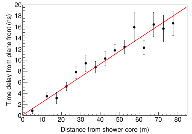
Figure 5: Shower front curvature of an EAS recorded on 1 January 2014. Number of triggered detectors is 261, size N_e = 8.9$\times$10⁴, age s = 1.21. A linear fit to the data represented by line yields a slope of 0.23 ns m^-1.

The profile of $\rm\delta t_{i}$ as a function of distance from the core of an EAS is shown in Fig. 5. The linear dependence of $\rm\delta t_{i}$ on distance from core is clear evidence of curvature which is well described by a conical shape. From a linear fit, the slope of the shower front ‘$\alpha$’ is 0.23 ns m^-1.

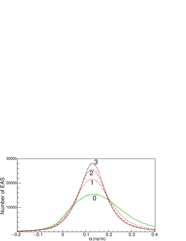
Figure 6: Distribution of shower front slope $\alpha$ from analysis of 2.4$\times$10⁶ EAS. (a) plot ‘0’ represents slope distribution, (b) ‘1’ after removal of outliers, (c) ‘2’ after removal of second round of outliers, (d) ‘3’ after removal of third round of outliers.

$\alpha$ is determined for each EAS for the data collected during 1–10 January 2014. Cuts imposed on EAS for this study include, $\rm\theta$$<$$40^{\circ}$, core within 30 m from the center of array. The distribution of $\alpha$ is shown by the plot labeled ‘0’ in Fig. 6. The mean and the root mean square deviation (rms) of the $\alpha$ distribution are 0.189 and 0.305 ns m^-1, respectively and its most probable value $\rm\alpha_{peak}$ is 0.141 ns m^-1. An examination of individual showers shows the presence of outliers which can significantly alter the fit and thereby influence the value of $\alpha$. This could be a factor contributing to the large width of $\alpha$. The outliers could be due to the noise in electronics, or from unassociated particles / delayed hadrons in the EAS etc. The following rigorous criteria are used to identify and iteratively remove the outliers. Prima facie $\rm\delta t_{i}$ with large deviation from the expected conical shower front may be treated as outliers. Since it is not possible to reliably estimate $\alpha$ by fitting individual showers because of the presence of outliers, $\rm\alpha_{peak}$ is used as the starting estimate for every EAS. The outliers are identified by calculating the time residuals for individual EAS by the following expression,

$$\rm\tau_{res}^{i}=\delta t_{i}-\alpha_{peak}\times r_{i}$$ (6)

Here, $\rm\alpha_{peak}$ = 0.141 ns m^-1 and r_i is distance of the i^th detector from EAS core. The mean ‘$\mu$’ and rms of residuals $\rm\tau_{res}^{i}$ are calculated for individual EAS. Thereafter, the data points with $\rm\tau_{i}$ such that $\rm\mu-(2\times rms)$ $>\tau_{i}>$ $\mu+(2\times rms)$ are termed the “outliers”. After removing outliers, each EAS is again reconstructed by fitting a plane and slope $\alpha$ recalculated. The distribution of $\alpha$ after the removal of outliers is shown by the plot labeled ‘1’ in Fig. 6. The mean value of $\alpha$ has decreased from 0.189 to 0.141 ns m^-1 after the first iteration of outlier removal. Moreover, the rms also decreased from 0.305 to 0.154 ns m^-1. This procedure for the removal of outliers and slope recalculation is repeated two more times to obtain new slope values after each iteration as shown in Fig. 6 by the plots labeled ‘2’, ‘3’ after the second and third iterations, repectively. After the second and third iterations, the mean remained virtually unchanged at 0.136 ns m^-1 and the rms evetually reduced to 0.132 ns m^-1. The fraction of detectors removed are 5%, 5% and 4% after first, second and third iterations, respectively. However, even after the third iteration, the rms is still large and compareble to the mean indicating that the slope possibly depends on other EAS parameters such as the size and age which are inverstigated next.

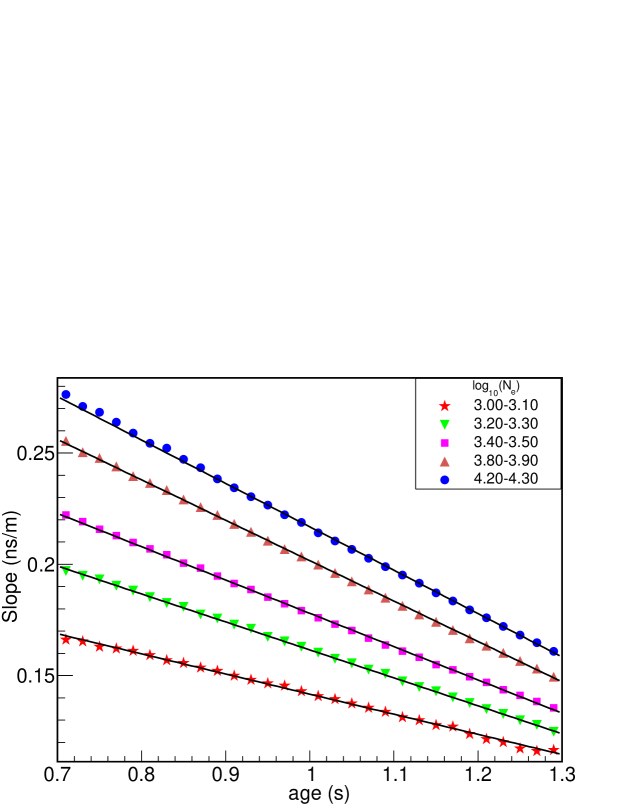
Figure 7: Dependence of slope $\alpha$ on EAS age (s) is shown for five size (N_e) groups.

For this analysis, the EAS recorded during the period from 1 January to 31 December 2014 are used. The following selection cuts are imposed on the data. Zenith angle ${\theta}$ is restricted below 40^∘ and the EAS cores should fall within 30 m from the array centre. A total of 8$\times$10⁷ EAS passed these cuts. Further, the EAS are categorized into 20 logarithmic size groups (each 10^0.1 wide) over the size range of 10³–10⁵. The variations of EAS slope $\alpha$ as a function of age ‘s’ for the five out of 20 size groups are shown in Fig. 7. The values of $\alpha$ are obtained after the third iteration of outlier removals. The following inferences can be drawn from the plots shown in Fig. 7, (i) for any given shower size the slope $\alpha$ systematically decreases with increasing age, (ii) for a given shower age, $\alpha$ is larger for higher shower size.

A linear fit provides an excellent description for the dependence of slope $\alpha$ on age (s) for each of the size group as seen from Fig. 7. From the linear fits to the data of 20 size groups the slope ‘M’ and intercept ‘C’ parameters are obtained for each case. Thus, the slope $\rm\alpha_{s}^{N_{e}}$ may be parameterized as,

$$\rm\alpha_{s}^{N_{e}}=M_{N_{e}}\times s+C_{N_{e}}$$ (7)

where $\rm M_{N_{e}}$ and $\rm C_{N_{e}}$ are the slope and intercept, respectively from the linear fit shown in Fig. 7.

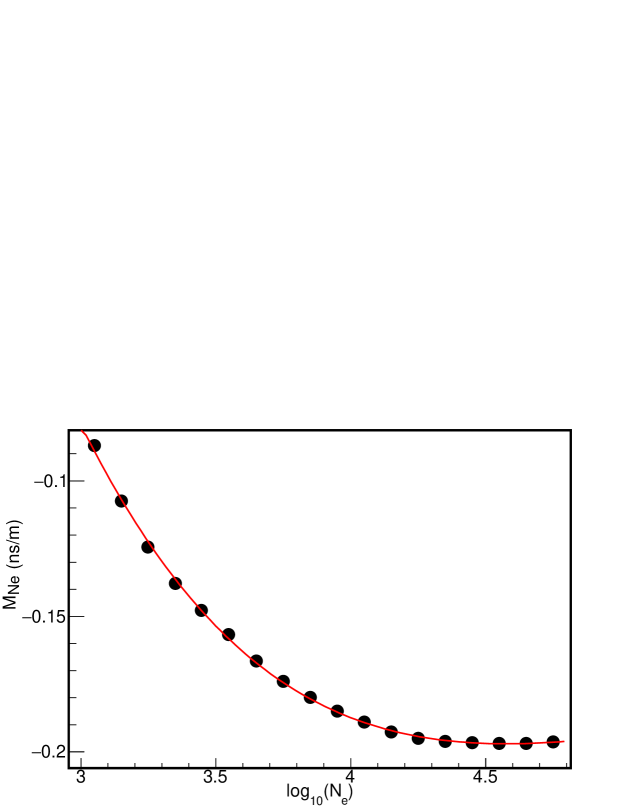
Figure 8: Dependence of $\rm M_{N_{e}}$ on shower size. $\rm M_{N_{e}}$ is the slope in the linear fit to the data displayed in Fig. 7.

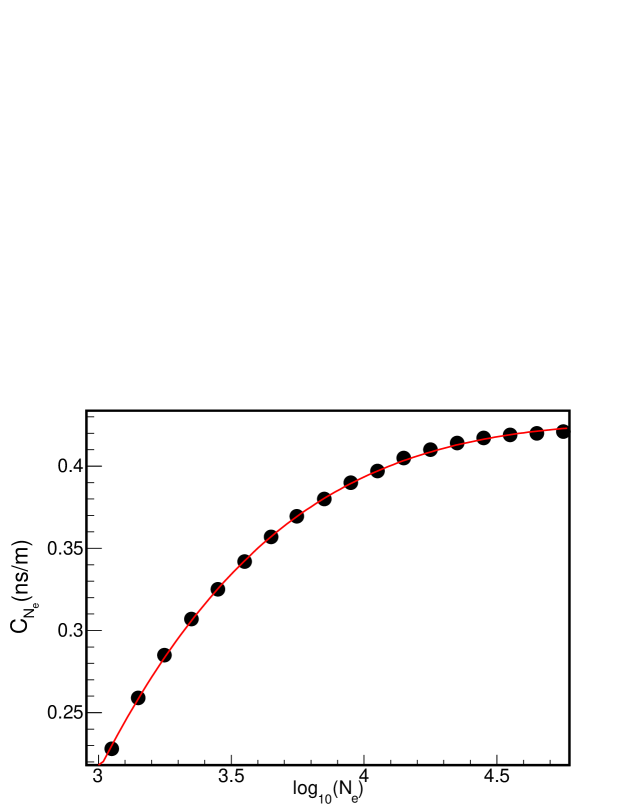
Figure 9: Dependence of $\rm C_{N_{e}}$ on shower size. $\rm C_{N_{e}}$ is intercept in the linear fit to data shown in Fig. 7.

Here, the parameter $\rm M_{N_{e}}$ and $\rm C_{N_{e}}$ represents the slope and intercept, repectively of the linear fit. In Fig. 8 the variation of parameter $\rm M_{N_{e}}$ with shower size is shown. The magnitude of $\rm M_{N_{e}}$ increases with increasing N_e, which indicates that the rapidity with which the slope $\alpha$ increases with age ‘s’ also increases with size N_e. Since the dependence of $\rm M_{N_{e}}$ on N_e apears to be somewhat similar to an exponential, an exponential fit was tried. However, these data required the use of two exponentials of the form, $\rm a_{1}\,exp(-b_{1}\,log_{10}N_{e})+c_{1}\,exp(-d_{1}\,log_{10}N_{e}^{2})-1$. The values of these parameters derived from the fit are, a₁ = 0.475 ns/m, b₁ = -0.036, c₁ = 1.792 ns/m and d₁ = 0.216. The fit to $\rm M_{N_{e}}$ obtained by using these parameters displayed in Fig. 8 shows excellent agreement between the data and the fit.

Similarly, the variation of intercept $\rm C_{N_{e}}$ as a function of N_e is shown in Fig. 9. This dependence also appears to be similar to an exponential and could be fitted well by a combination of two exponential functions given by $\rm 1-a_{2}\,exp(-b_{2}\,log_{10}N_{e})-c_{2}\,exp(-d_{2}\,(log_{10}N_{e})^{2})$. The parameters from this fit are, a₂ = 0.528 ns/m, b₂ = -0.081, c₂ = 1.014 ns/m, d₂ = 0.159. This analysis clearly shows that the shower front curvature is not a constant but varies from shower to shower and yet can be uniquely estimated from the knowledge of EAS size and age. The main objective of this study is to investigate if such a parametrization of shower front curvature could actually lead to significant improvement in the angular resolution of the array. The impact of shower dependent curvature correction is qunatitatively examined in the next section.

4 Angular resolution of GRAPES-3 array

Figure 10: A schematic representing the biased direction due to the presence of shower front curvature with left-right method.

In §3, a detailed study of the shower front curvature showed that its dependence on the EAS size and age can be easily parametrized. Here, the EAS direction is corrected for shower front curvature and the effect of this correction on the angular resolution of the array is investigated. For this purpose two independent techniques of dividing the array into, (i) the “odd” and “even” numbered detectors, (ii) a “left” and a “right” sub-arrays are implemented. The details of these two techniques are described in an earlier work from GRAPES-3 experiment [25].

The scintillator detectors in the GRAPES-3 array are deployed with a hexagonal geometry as shown in Fig. 1. These detectors are labeled sequentially, starting from the centre of the array and thereafter proceeding clockwise along the first hexagonal ring, followed by the second ring and so on. For the odd-even method, the GRAPES-3 array is divided into two sub-arrays. Each sub-array comprises of either “odd” or “even” numbered detectors. By using the plane shower front independent estimate of the arrival direction is obtained from the “odd” ($\theta_{o}$,$\phi_{o}$) and “even” ($\theta_{e}$,$\phi_{e}$) sub-arrays. Next, the space angle $\psi_{oe}$ between these two directions is calculated. The distribution of $\psi_{oe}$ provides a measure of the angular resolution of the array by the odd-even method. For the left-right method, the array is divided into a “left” and a “right” sub-array by the following criterion. For each shower, a line joining its core and the array center is used as the dividing line for the two sub-arrays. Therefore, unlike the odd-even method, the detectors in the “left” and “right” sub-arrays change with every shower according to the location of the core.

The space angle $\psi_{lr}$ between the two directions measured by the “left” ($\theta_{l}$, $\phi_{l}$) and “right” ($\theta_{r}$, $\phi_{r}$) sub-arrays would be used for further analysis. The distribution of $\psi_{lr}$ can not be used as a measure of the angular resolution because of the contribution from the shower front curvature. This curvature results in a systematic tilt of the reconstructed “left” and “right” directions as shown schematically in Fig. 10 for a conical shower front. This systematic tilt between “left” and “right” directions can be used to estimate the shower front curvature on a event by event basis. On the other hand, the odd-even method is not sensitive to the existence of shower front curvature. This is because the “odd” and “even” sub-arrays are basically two overlapping arrays each with half the detectors. Thus, for a curved shower front both the sub-arrays provide directions which may be inaccurate, but both point in the same incorrect direction within the angular resolution of the arrays. In summary, the angle $\psi_{oe}$ provides an estimate of the best achievable angular resolution because it only contains the statistical errors since the systematic errors are eliminated because of the overlapping nature of the two sub-arrays. Consequently, odd-even method can not provide the absolute direction of an EAS. On the other hand, if appropriate correction can be made for the shower front curvature then the left-right method provides the correct and absolute direction of an EAS relative to the local frame of reference.

For the left-right study, the direction of each EAS ($\theta$, $\phi$) is obtained by fitting a plane shower front as given in Eq. 1. Next, by using the size and age of the EAS as described in §3, the slope of shower front curvature is calculated by assuming it to be cone shaped and corrected as follows,

$$\rm t_{c}^{i}=t_{m}^{i}-r_{i}\times\alpha_{s}^{N_{e}}$$ (8)

Here $\rm t_{m}^{i}$ are measured arrival times, ${\rm r_{i}}$ distances of the i^th detector from the shower core, ${\rm\alpha_{s}^{N_{e}}}$ the size and age dependent slope of the shower curvature as described in §3. Therefore, the arrival times $\rm t_{c}^{i}$ obtained after the removal conical shower front curvature, effectively represents a plane shower front. Therefore, the EAS direction ($\theta$, $\phi$) can be obtained by a plane fit. Following the plane fit the outliers in the data are iteratively removed as described in §3.

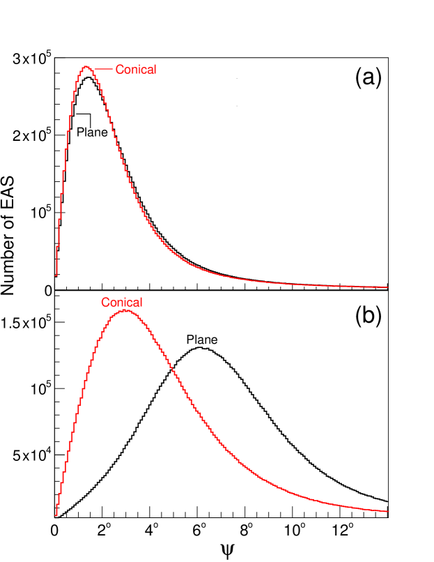
Figure 11: Distribution of space angles $\psi$, between two sub-arrays for, (a) odd-even for plane and conical fits, (b) left-right also for plane and conical fits for shower size $>$10^4.0.

The distribution of space angle between the “odd” and “even” sub-arrays for the shower size $\geq$10^4.0 for plane and conical shower fronts are shown in Fig. 11a. These the two distributions appear indistingushable which is not surprising the two sub-arrays are nearly identical and fully overlap and therefore, the EAS directions measured by them contain identical systematic effects which get eliminated when the space angle between them is measured. Thus, the width of the distribution in Fig. 11a reflects the true angular resolution of the sub-arrays.

However, when this procedure is repeated for the “left” and “right” sub-arrays, the outcome is completely different as shown in Fig. 11b. The distribution for the Plane front fit is almost a factor of two wider than for the conical shower front as seen in Fig. 11b. This clearly shows that the shower curvature plays a significant in direction reconstruction and the curvature correction can improve the angular resolution of the array.

Figure 12: Distribution of space angle $\rm\psi_{lr}$ by left-right method for N${}_{e}\,>\,$10⁴ after iterative outlier removals, (i) ‘0’ without outlier removal, (ii) ‘1’ first, (iii) ‘2’ second, (iv) ‘3’ third iteration of outlier removals, respectively.

As discussed earlier in §3, the outliers in the data significantly degrade the measurement of arrival direction of an EAS by the left-right method, thereby influencing the achievable angular resolution of the array. To improve the resolution, direction reconstruction needs to be carried out after iterative removal of the outliers as described in §3 and the resulting histograms are shown in Fig. 12 for shower size N${}_{e}\,>\,$10⁴. The width of each histogram is representative of the angular resolution achieved. Histograms labeled, (i) ‘0’ is without outlier removal, (ii) ‘1’ after the first round of outlier removal, (iii) ‘2’ after the second round of outlier removal, (iv) ‘3’ after the third round of outlier removal. A reduction in the width of the histogram indicating corresponding improvement in the angular resolution of the array is observed after each round of outlier removal. The distribution becomes significantly narrower after the first round of outlier removal and the improvement is more modest after the second and third round. No measureable reduction in the histogram width is observed after the fourth and higher rounds of outlier removal. Consequently, only three iterations of outlier removal are carried out hereafter.

The distribution of space angle $\rm\psi$ obtained from the two sub-arrays is converted into a density distribution by dividing the contents of each angular bin by its solid angle. If $\rm\psi_{low}$ and $\rm\psi_{upper}$ are the lower- and upper boundaries of an angular bin, then its solid angle is, cos$\rm\psi_{low}$ – cos$\rm\psi_{upper}$. The two density distributions as a function of space angles $\rm\psi$ for the odd-even and left-right sub-arrays, respectively are shown in Fig. 13 for shower size N${}_{e}\,\geq\,10^{4.0}$. The angular resolution of an array can be defined in a variety of ways. For a Gaussian density distribution, it can be shown that the maximum signal to noise (S/N) ratio for a point source occurs for an opening space angle $\rm\psi_{0}$ = 1.6$\times\sigma$, where $\sigma$ is the standard deviation of corresponding density distribution. Alternatively, for a point $\gamma$-ray source the maximum S/N ratio after the reconstruction of showers would occur for a space angle of $\rm\psi_{0}$ centred on the source direction. This relation is used subsequently to estimate the angular resolution $\sigma$ of the GRAPES-3 array given by $\sigma$ = $\rm\psi_{0}$/1.6 [16, 27]. For the odd-even method, each sub-array covers nearly the full area of array, except that (i) the number of detectors are halved, (ii) the space angle $\rm\psi$ contains errors from measurements by each of the two sub-arrays. These two effects increase the errors by a factor of $\sqrt{2}$ each, and therefore, the true error $\rm\sigma_{oe}$ is a factor of $\sqrt{2}\times\sqrt{2}$ = 2 smaller than the measured error $\sigma_{1}$ obtained from a Gaussian fit to the histogram labeled ‘odd-even’ in Fig. 13. On the other hand, for the left-right method, apart from the two effects mentioned above, there is a third effect due to the decrease in the area of each sub-array by a factor of two. Thus, the true error $\rm\sigma_{lr}$ is a factor of 2$\sqrt{2}$ smaller than the measured $\sigma_{2}$ obtained from a Gaussian fit to the histogram labeled ‘left-right’ in Fig. 13 and thus,

$$\rm\sigma_{1}\,=\,\sqrt{2}\times\sigma_{2}$$ (9)

As discussed above, the density distribution for the left-right method shown in Fig. 13 should be broader than the odd-even method by a factor $\sqrt{2}$ = 1.41. The Gaussian fits to the two density distributions shown in Fig. 13 yield, $\rm\sigma_{1}$ = 0.74^∘ and $\rm\sigma_{2}\,=\,1.06^{\circ}$ which yields a ratio of 1.43 which is close to the expected value of 1.41.

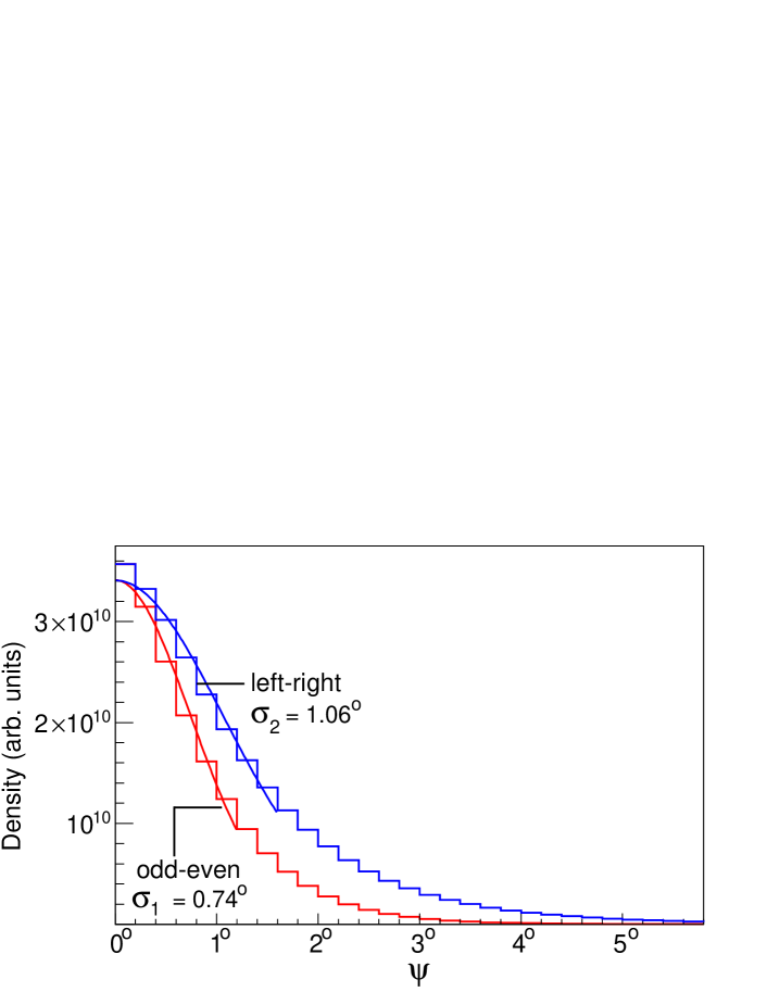
Figure 13: Event density per unit solid angle as a function of space angle $\psi$ for N${}_{e}>$10^4.0 for the left-right sub-arrays.

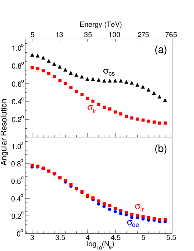
Figure 14: Variation of angular resolution as a function of shower size N_e for (a) a constant shower front curvature determined with size and age dependent slope and fixed slope for left-right method as a function of integral shower size.

In Fig. 14a the variation of angular resolution $\sigma_{cs}$ of the GRAPES-3 array obtained by using a constant slope of 0.129 ns m^-1 for the shower front curvature, after three iterations of outlier removal is shown. The angular resolution $\sigma_{cs}$ decreases from 0.92^∘ (55^′) for size N$\rm{}_{e}>10^{3.0}$ to 0.42^∘ (25^′) for N$\rm{}_{e}>10^{5.5}$. Next, the variation of $\sigma_{lr}$ after the corrections for the size and age dependent shower front curvature and three rounds of iterative removal of outliers is shown in Fig. 14a. $\sigma_{lr}$ decreases from 0.8^∘ (47^′) to just below 0.16^∘ (10^′) over the same shower size range. Clearly the angular resolution measured after the size and age dependent correction is significantly better than the constant slope correction generally used. The improvement is especially significant for higher shower sizes.

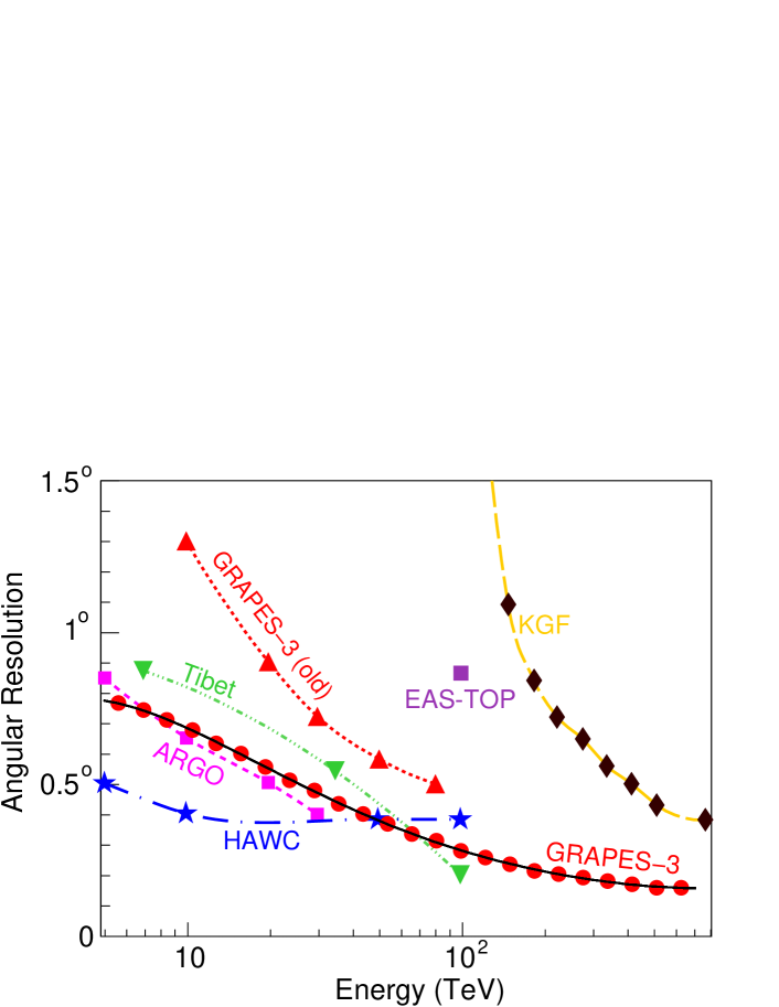
Figure 15: Variation of angular resolution with PCR energy for following arrays, (1) KGF 100–800 TeV [16], (2) EAS-TOP 100 TeV [28], (3) GRAPES-3 10–80 TeV old analysis [25], (4) Tibet AS$\gamma$ 7–100 TeV [30], (5) ARGO-YBJ 5–30 TeV [29], (6) HAWC 5–100 TeV [31], (7) GRAPES-3 5–800 TeV present analysis.

As mentioned earlier, the odd-even method provides the best achievable angular resolution because this method eliminates common systematic errors and only the statistical uncertainties in the data survive. In Fig. 14b the angular resolution $\rm\sigma_{oe}$ obtained by the this method is shown as a function of the shower size. $\rm\sigma_{oe}$ varies from 0.76^∘ (46^′) to 0.13^∘ (8^′) over the same size range. The angular resolution $\rm\sigma_{lr}$ obtained by the left-right method as a function of shower size is overlaid in Fig. 14b. The two methods display very similar bahviour, clearly indicating that the use of real time TDCZeros as well as the size and age dependent shower front curvature correction resulted in not only a sizable improvement in the angular resolution, but also the systematic effects are almost completely eliminated. Thus, the angular resolution is now dominated by the statistical uncertainties present in the GRAPES-3 data obtained by the odd-even method.

5 Discussions

Worldwide, a number of experiments have been operated to detect multi-TeV $\gamma$-ray sources. The experiments that are no longer collecting data include the KGF, the EAS-TOP and the ARGO-YBJ arrays. Located at an atmospheric depth of 920 g.cm^-2 the angular reolution of KGF array as a function of PCR energy displayed by symbol $\blacklozenge$ in Fig. 15 varies from 1.1^∘ at $>$150 TeV to 0.4^∘ at $>$800 TeV [16]. The dashed line joining the data is not a fit but meant to guide the eye. The EAS-TOP array (atmospheric depth 820 g.cm^-2) had an angular resolution of 0.9^∘ at $>$100 TeV shown by symbol $\blacksquare$ in Fig. 15 [28]. The ARGO-YBJ (depth 600 g.cm^-2), a sophisticated RPC based carpet array had an angular resolution that varied from 0.9^∘ at $>$5 TeV to 0.4^∘ at $>$30 TeV shown by the symbol $\blacksquare$ in Fig. 15 [29].

The EAS arrays operating currently include the Tibet AS$\gamma$, the HAWC water Cherenkov and of course the GRAPES-3. The angular resolution of Tibet AS$\gamma$ array (depth 600 g.cm^-2) varies from 0.9^∘ at $>$7 TeV to 0.2^∘ at $>$100 TeV shown by symbol $\blacktriangledown$ in Fig. 15 [30]. Interestingly, the angular resolution of HAWC array (depth 600 g.cm^-2) varies within a narrow range of 0.5^∘–0.4^∘ in the energy range $>$5–100 TeV as shown by symbol $\bigstar$ in Fig. 15 [31]. The angular resolution of GRAPES-3 (depth 800 g.cm^-2) by using the old method varied from 1.3^∘ at $>$10 TeV to 0.5^∘ at $>$80 TeV as shown by symbol $\blacktriangle$ in Fig. 15. But the new real time TDCZero as well as size and age dependent shower front curvature correction led to a significant improvement in the resolution, compared to the previous analysis [25]. The angular resolution improved from 1.3^∘ to 0.7^∘ at $>$10 TeV and from 0.5^∘ to 0.3^∘ at $>$80 TeV in the new analysis as shown by symbol ${\bullet}$ in Fig. 15. In view of the sub-degree values, hereafter the angular resolution of the GRAPES-3 shall be quoted in arc-minutes.

But even more significantly this analysis has permitted the reconstruction of showers of energies as low as $>$5 TeV with a respectable resolution of 47^′ by the GRAPES-3 array located deep in the atmospheric at a depth of 800 g.cm^-2. This might prove to be a critical factor in the detection of TeV $\gamma$-ray sources, most of which show steepening of energy spectrum in the TeV region. The EAS-TOP array too had operated at an atmospheric depth similar to the GRAPES-3, yet the GRAPES-3 angular resolution is a factor of three better [28] as shown in Fig. 15. The angular resolution of GRAPES-3 is comparable to that of ARGO-YBJ [29] and Tibet AS$\gamma$ [30] as shown in Fig. 15, despite the fact that both these arrays are located at 200 g.cm^-2 shallower depth than GRAPES-3. Only the large HAWC array [31] also located 200 g.cm^-2 shallower than GRAPES-3 provides a better resolution than the GRAPES-3 in 5–50 TeV region. But above 50 TeV, GRAPES-3 delivers a slightly better performance. The key takeaways from this analysis which is based on the use of real time TDCZeros as well as size and age dependent shower front curvature corrections are, (i) For similar atmospheric depths, the method described here yields a better angular resolution, (ii) The improvement in angular resolution is equivalent to arrays operating at 200 g.cm^-2 shallower depths.

6 Conclusions

A new method has been developed to determine the real time delay caused by the photomultiplier tubes, co-axial cables, and electronics in each detector of the array by using a statistical approach. This is followed by an accurate modeling of the shower front curvature using the data collected by the GRAPES-3 array during 2014. This data showed that shower front curvature can be modeled by a conical shape which depends on the shower size and age. This dependence is accurately parametrized in the GRAPES-3 data. The shower front curvature shows clear dependence both on the shower size and age. The correction for this curvature allowed the GRAPES-3 array to achieve an angular resolution which is dictated primarily by the uncertainties in the data. The angular resolution varies from 47^′ at $>$5 TeV to 10^′ at $>$500 TeV. These values compare favourably with the arrays such as ARGO-YBJ, Tibet AS$\gamma$ and HAWC located at higher elevations than GRAPES-3 where the atmospheric depth is 200 g.cm^-2 shallower. This method if applied to existing arrays might lead to improvement in their angular resolution and thereby enhance their sensitivity for the discovery of fainter $\gamma$-ray sources.

References

References

- [1] T.K. Gaisser, R. Engel and E. Resconi, Cosmic Ray and Particle Physics, Cambridge Univ. Press. ISBN: 978-0-521-01646-9 (2016).
- [2] S. Funk, Ground- and Space-Based Gamma-Ray Astronomy, Ann. Rev. Nucl. Part. 65 (2015) 245.
- [3] F. Ahronian et al., Primary particle acceleration above 100 TeV in the shell-type supernova remnant RX J1713.7-3946 with deep HESS observations, Astron. Astrophys. 464 (2007) 235.
- [4] M. Amenomori et al., First Detection of Photons with Energy beyond 100 TeV from an Astrophysical Source, Phys. Rev. Lett. 123 (2019) 051101.
- [5] H. Abdalla et al., H.E.S.S. observations of RX J1713.7−3946 with improved angular and spectral resolution: Evidence for gamma-ray emission extending beyond the X-ray emitting shell, Astron Astrophys. 612 (2018) A6.
- [6] J. Aleksic et al., The major upgrade of the MAGIC telescopes, Part II: A performance study using observations of the Crab Nebula, Astropart. Phys. 72 (2016) 76.
- [7] N. Park et al., Performance of the VERITAS experiment, POS (ICRC2015) (2015) 771.
- [8] P. Bassi, G. Clark, and B. Rossi, Distribution of Arrival Times of Shower Particles, Phys. Rev. 92 (1953) 441.
- [9] J. Linsley et al., EXTREMELY ENERGETIC COSMIC-RAY EVENT, Phys. Rev. Lett. 6 (1961) 485.
- [10] V.I. Kozlov et al., THE RESULTS OF THE FIRST STAGE OBSERAVATIONS AT THE YAKUTSK EAS COMPLEX ARRAY. III.ZENITH ANGLE EAS DISTRIBUTION WITH SIZE PARTICLES AT THE SEA LEVEL AND STRONGLY INCLINED EVENTS OF LARGE SIZES, Proc. 13th Int. Cosmic Ray Conf. Denver 4 (1973) 2588.
- [11] T. Hara et al., Characteristics of Large Air Showers at core distances between 1km and 2km, Proc. 18th Int. Cosmic Ray Conf. Bangalore 11 (1983) 276.
- [12] R. Haeusler et al., Distortions of experimental muon arrival time distributions of extensive air showers by the observation conditions, Astropart. Phys. 17 (2002) 421.
- [13] B. D’Ettorre Piazzoli et al., Monte Carlo simulation of photon-induced air showers, Astropart. Phys. 2 (1994) 199.
- [14] G. Battistoni et al., Monte Carlo study of the arrival time distribution of particles in extensive air showers in the energy range 1-100 TeV, Astropart. Phys. 9 (1998) 277.
- [15] P.K.F Greider, Cosmic Ray at Earth, Elsevier ISBN: 0-444-50710-8 (2001).
- [16] B.S. Acharya et al., Angular resolution of the KGF experiment to detect ultra high energy gamma-ray sources, J. Phys. G Nucl. Part. Phys. 19 (1993) 1053.
- [17] M. Ambrosio et al., Time structure of individual extensive air showers , Astropart. Phys. 11 (1999) 437.
- [18] G. Agnetta et al., Time structure of the extensive air shower front, Astropart. Phys. 6 (1997) 301.
- [19] T. Antoni et al., Time structure of the extensive air shower muon component measured by the KASCADE experiment, Astropart. Phys. 15 (2001) 149.
- [20] A.K. Calabrese Melcarne et al., Study of cosmic ray shower front and time structure with ARGO-YBJ, J. Phys.: Conf. Ser. 409 (2013) 012049.
- [21] S. K. Gupta et al., GRAPES-3–A high-density air shower array for studies on the structure in the cosmic-ray energy spectrum near the knee, Nucl. Instrum. Meth. A 540 (2005) 311.
- [22] P.K. Mohanty et al., Measurement of some EAS properties using new scintillator detectors developed for the GRAPES-3 experiment, Astropart. Phys. 31 (2009) 24-26.
- [23] Y. Hayashi et al., A large area muon tracking detector for ultra-high energy cosmic ray astrophysics–the GRAPES-3 experiment, Nucl. Instrum. Meth. A 545 (2005) 643.
- [24] S.K. Gupta et al., Measurement of arrival time of particles in extensive air showers using TDC32, Expt. Astron. 35 (2012) 507.
- [25] A. Oshima et al., The angular resolution of the GRAPES-3 array from the shadows of the Moon and the Sun, Astropart. Phys. 33 (2010) 97.
- [26] H. Tanaka et al., Studies of the energy spectrum and composition of the primary cosmic rays at 100–1000 TeV from the GRAPES-3 experiment, J. Phys. G: Nucl. Part. Phys. 39 (2012) 025201.
- [27] L.J. Graham, Ultra high energy gamma ray point sources and cosmic ray anisotropy, Ph.D Thesis, Univ. of Durham (1994) unpublished, http://etheses.dur.ac.uk/5594
- [28] M. Aglietta et al., DETECTION OF THE SHADOW OF THE SUN AND THE MOON ON 100 TeV COSMIC RAYS (EAS-TOP DATA), Proc. of 22nd Cosmic Ray Conf 2 (1991) 708.
- [29] G. Aielli et al., Highlights from the ARGO-YBJ experiment, Nucl. Instrum. Meth. A 661 (2012) 550.
- [30] M. Amenomori et al., Cosmic-ray deficit from the directions of the Moon and the Sun detected with the Tibet air-shower array, Phys. Rev. D 47 (1993) 2675; M. Amenomori et al., First Detection of Photons with Energy beyond 100 TeV from an Astrophysical Source, Phys. Rev. Lett. 123 (2019) 051101.
- [31] R. Alfaro et al., All-particle cosmic ray energy spectrum measured by the HAWC experiment from 10 to 500 TeV, Phys. Rev. D 96 (2017) 122001.