Residual Smoothing: Using Mocks to Correct Model Covariance Matrices

Abstract

Covariance matrix estimation is a challenging problem in cosmology. Recent work has shown that model covariance matrices can be precise, and that at relatively large scales they can also be accurate. We introduce a data-driven method that can identify features from a mock covariance matrix that are missing from a corresponding model, then incorporate them into the model without significantly degrading the model’s precision. We apply this method to a BOSS-like survey and extend a model covariance to be valid at scales relevant for measurements of Redshift Space Distortions ($8-40\,h^{-1}\text{Mpc}$), where the galaxy field is significantly non-Gaussian.

1 Introduction

Covariance matrix estimation is a necessary part of many cosmological analyses. It is a challenging problem because we have only one sky to observe, and so cannot directly generate multiple sets of independent observations. See [1, 2, 3] for foundational work explicating the covariance matrix problem, and [4, 5, 6, 7, 8, 9, 10, 11, 12, 13, 14] for some of the recent work that addresses the problem.

Broadly speaking, there are two ways to solve this problem. The first is to generate reasonably accurate numerical simulations of the evolution of the universe, or “mocks”, and perform sample statistics with the mocks. The resulting covariance matrix is often assumed to be accurate, but suffers from challenging trade-offs between the number of mocks generated (with each being computationally expensive) and the level of noise on the final covariance matrix. The other approach is to use theoretical insights to produce an analytic or semi-analytic model covariance matrix. These approaches generally feature high precision at minimal computational expense, but the accuracy of the resulting covariance matrix rests on the underlying theoretical model, which may be incomplete or inaccurate.

In this note we introduce a simple method to reconcile the numerical and theoretical approaches. We assume that both mocks and a model covariance matrix are available, focus our attention on the residual difference between the two, then smooth that residual. We then add the smoothed residual back to the original model covariance matrix to achieve a result that combines the accuracy of the mocks with the precision of the model. Our improvements rest on the validity of the smoothing technique; we use the Kullback-Leibler divergence, a robust tool from information theory, to track the quality of the resulting covariance matrix, and cross-validation to limit the degree of overfitting/undersmoothing.

We demonstrate this approach on a BOSS-like galaxy survey. In [15] we developed a model covariance matrix that is largely Gaussian, and incorporates short-scale non-Gaussianity through a shot-noise rescaling parameter. This model was found to be accurate at separations relevant for measurements of baryon acoustic oscillations (BAO) ($\gtrsim 80\,h^{-1}\text{Mpc}$), but at separations relevant for measurements of redshift space distortions (RSD) ($\lesssim 40\,h^{-1}\text{Mpc}$) its accuracy was compromised, presumably because it did not incorporate mid-scale non-Gaussianity of the galaxy field. Applying residual smoothing we are able to correct the model and restore these non-Gaussian contributions.

In Section 2 we introduce the family of projection operators that are used to smooth the residual. If the correlation function is estimated in $n$ bins, then this family is $2^{n}$-dimensional. In Section 3 we develop an algorithm to identify relevant members of this family and assess their performance. In Section 4 we apply the method to a BOSS-like survey and see that it identifies necessary corrections to the model covariance matrix with minimal overfitting. We conclude in Section 5.

2 Projection Operators and Smoothing

Suppose that we have a model covariance matrix, $C_{\text{model}}$, and a covariance matrix computed from a modest number of mocks, $C_{\text{sample}}$. We define the residual between these covariance matrices as

$$\Delta=C_{\text{sample}}-C_{\text{model}}\,.$$ (1)

The residual $\Delta$ can non-zero both because of noise in $C_{\text{sample}}$, and also because of bias in $C_{\text{model}}$ relative to $C_{\text{sample}}$. Our goal is to generate $\tilde{\Delta}$, a smoothed version of $\Delta$, which minimizes the contributions from noise and isolates the bias of $C_{\text{model}}$ relative to $C_{\text{sample}}$. We can then use $C_{\text{model}}+\tilde{\Delta}$ as an improved covariance matrix estimate, with less bias than $C_{\text{model}}$ alone and less noise than $C_{\text{sample}}$.

We will use projection operators to smooth $\Delta$. Mathematically, a projection operator $\Pi$ is idempotent,

$$\Pi^{2}=\Pi\,.$$

The intuition is that the operator restricts to a subspace, and that subsequent applications of the projection operator do not produce any further change. In our case the projection operators will be matrices of the same shape as the covariance matrix, and will act on the residual as

$$\tilde{\Delta}=\Pi\Delta\Pi^{T}\,.$$ (2)

We then combine the smoothed residual $\tilde{\Delta}$ with the original model to yield the corrected model,

$$\tilde{C}=C_{\text{model}}+\tilde{\Delta}\,.$$ (3)

In order for projection to lead to smoothing, we must be able to identify a subspace that contains the bulk of the bias in $C_{\text{model}}$ while excluding most of the noise from $C_{\text{sample}}$.

The family of projection operators that we consider are built from eigenvector decompositions of matrices. Suppose that an $n\times n$ symmetric matrix $C$ is decomposed as

$$C=Q\times\text{diag}\left(\lambda_{1},\lambda_{2},\dots,\lambda_{n}\right)\times Q^{T}\,,$$ (4)

where the $i$th column of $Q$ is the $i$th eigenvector of $C$, and $\lambda_{i}$ is the $i$th eigenvalue of $C$. We can construct a large family of projection operators as

$$\Pi=Q\times\text{diag}\left(\delta_{1},\delta_{2},\dots,\delta_{n}\right)\times Q^{T}\,,$$ (5)

where $\delta_{i}$ is either one or zero. A familiar example of this approach would be to set $\delta_{i}=1$ for the $k$ largest eigenvalues and $\delta_{i}=0$ otherwise. The resulting projection operator would pick out the same $k$-dimensional subspace that would emerge from principal component analysis (PCA).

We have three candidates sources for the eigenvectors $Q$: $C_{\text{sample}}$, $C_{\text{model}}$, and $\Delta$. Our goal is to cleanly separate bias from noise, which is difficult to do if the eigenvectors themselves have a significant amount of noise. For that reason we will use the eigenvectors of $C_{\text{model}}$. While $C_{\text{model}}$ and $\Delta$ are qualitatively different from one another, they share many important features pertaining to bin ordering, scaling, etc., and so the eigenvectors from $C_{\text{model}}$ can efficiently capture the features of $\Delta$.

After choosing the eigenvectors $Q$, we need to determine which $\delta_{i}$ should be non-zero. Note that because $C_{\text{model}}$ and $\Delta$ are quite different matrices, we do not expect (and in the following do not find) that the leading eigenvectors are the ones that should be included in the final subspace (i.e. have $\delta_{i}=1$). Rather we must search among the $2^{n}$ possible projection operators to identify the one that provides the optimal projection.

3 Learning the Projection Operator

In this section we describe in detail our method for identify the preferred projection operator. Broadly speaking, there are two parts to this procedure. First, we repeat the following many times:

1. Randomly split the available mocks into equal training and test sets, compute sample covariance matrices $C_{\text{training}}$ and $C_{\text{test}}$.

2. Invert $C_{\text{test}}$ and apply the usual Wishart correction to find $\Psi_{\text{test}}$.

3. Compute the residual $\Delta=C_{\text{training}}-C_{\text{model}}$.

4. Apply the Metropolis-Hastings algorithm to the $\delta_{i}$ to find a projection operator that minimizes the Kullback-Leibler (KL) divergence, $\text{KL}\left(\tilde{C},\Psi_{\text{test}}\right)$. The KL divergence is described below in Section 3.1.

The repeated splitting of mocks into training and test sets is known as Monte Carlo cross-validation. For any particular split we will find a large number of modes included in the optimal projection operator. By iterating over splits we can better identify which modes consistently appear, and which modes appear infrequently and are associated with noise.

Because our final projection operator must have only 0’s and 1’s for the $\delta_{i}$, we cannot simply average the results of each run to find a consensus projection operator. Instead we track how many times each mode was included in an optimal projection operator, producing a ranking of the modes. In the final projection operator modes are included according to that ranking. A second round of cross-validation, described in Section 3.2, determines how many of those modes to include.

We use Monte Carlo cross-validation in order to reduce overfitting of the projection operator. As we are comparing statistically independent training and test sets, the projection operator should not be able to adapt to noisy features in the training set. However, we assume a limited number of mocks are available, and so noisy features in the entire set of mocks will be split between the training and test sets for each iteration of Monte Carlo cross-validation. This opens the door to a limited amount of overfitting, and we will see in Section 4 that it has a modest impact on our results.

3.1 The Kullback-Leibler Divergence

To quantify the difference between a proposed covariance matrix and a sample covariance matrix, we use the Kullback-Leibler (KL) divergence [16]. The KL divergence is a tool from information theory that provides a natural measure of the dissimilarity between two distributions. For two multivariate-normal distributions with the same mean, it takes a simple form,

$$\text{KL}\left(C_{1},\Psi_{2}\right)=\frac{1}{2}\left[\text{tr}\left(C_{1}\Psi_{2}\right)-\log\left(\det\left(C_{1}\right)\right)-\text{log}\left(\text{det}\left(\Psi_{2}\right)\right)-n\right],$$ (6)

where $C_{1}$ is the $n\times n$ covariance matrix of the first distribution and $\Psi_{2}=C_{2}^{-1}$ is the precision matrix of the second distribution. When $C_{1}$ and $\Psi_{2}$ are known exactly, larger values of the KL divergence correspond to greater differences between the two matrices. If, on the other hand, $C_{1}$ is a sample covariance computed from $n_{s}$ samples whose true covariance matrix is $C_{2}$, then $\text{KL}\left(C_{1},\Psi_{2}\right)\sim n^{2}/4n_{s}$, so noise also increases the KL divergence.

3.2 How many modes?

As described above, the first round of cross-validation tells us how often each mode is included in an optimal projection operator. At this we could apply an arbitrary cut on frequency, perhaps after looking at the results of the first round of cross-validation, and have a useful projection operator. Here we develop a more systematic approach. Our goal is to automatically determine the optimal number of modes to include, and thus the optimal projection operator.

For the second round of cross-validation we repeat the following many times:

1. Randomly split the available mocks into equal training and test sets, compute sample covariance matrices $C_{\text{training}}$ and $C_{\text{test}}$.

2. Invert $C_{\text{test}}$ and apply the usual Wishart correction to find $\Psi_{\text{test}}$.

3. Compute the residual $\Delta=C_{\text{training}}-C_{\text{model}}$.

4. For each $k$ of interest, construct a projection operator $\Pi_{k}$ with $\delta_{i}=1$ for the $k$ highest-ranked modes. Use it to generate a corrected model $\tilde{C}_{k}$.

5. Compute $\text{KL}\left(\tilde{C}_{k},\Psi_{\text{test}}\right)$ for each $k$ of interest.

Having found the distribution of KL divergences for each value of $k$, it is then straightforward to determine which $k$ leads to the smallest KL divergence, and is therefore optimal.

Our general expectation is that the first few modes will bring $\tilde{C}$ closer to $\mathbf{E}\left[C_{\text{sample}}\right]$, reducing the KL divergence. As we add more modes the smoothed residual $\tilde{\Delta}$ incorporates more of the noise of $C_{\text{test}}$, and so we expect the KL divergence to eventually increase. Competition between these two effects would then produce an isolated minimum in the KL divergence as a function of $k$. In cases where $C_{\text{model}}$ is already very close to $\mathbf{E}\left[C_{\text{sample}}\right]$ it is possible that this minimum will happen at $k=0$, indicating that we should simply use the uncorrected $C_{\text{model}}$.

4 Application to a BOSS-like survey

To demonstrate the efficacy of this approach we use 1,000 QPM mocks [17], generated for the analysis of the NGC portion of the BOSS survey [18], and a model covariance matrix generated using Rascal [15] for the same survey. We will consider a correlation function estimated in $r-\mu$ coordinates, estimated in bins of width $\Delta r=4\,h^{-1}\text{Mpc}$ and $\Delta\mu=0.1$. The model covariance includes a shot-noise rescaling parameter $a=1.06$, in agreement with previous work [19].

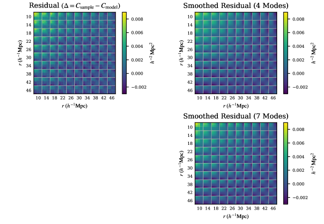
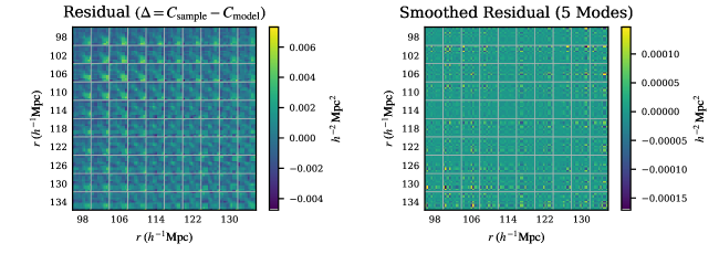
We consider two ranges of $r$-values. The high-$r$ range encompasses 100 bins over $r=96-136\,h^{-1}\text{Mpc}$. This is a range of separations where we expect the galaxy field to be very Gaussian, and is relevant for measurements of baryon acoustic oscillations (BAO). In previous work we have found the model covariance matrix to be quite accurate [15], and so we anticipate a smoothed residual that is small or zero. The low-$r$ range includes 100 bins over $r=8-48\,h^{-1}\text{Mpc}$. This range of scales is relevant for measurements of redshift space distortions (RSD). It is also a range of scales where the galaxy field is significantly non-Gaussian, and consequently we expect that the model covariance matrix will be biased. The smoothed residual should reduce or eliminate this bias, extending the model covariance matrix to a previously inaccessible range of $r$.

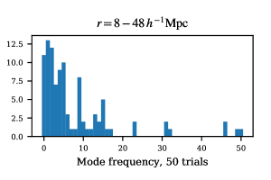
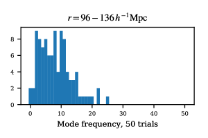
We begin by using Monte Carlo cross-validation to identify relevant modes, as described in Section 3, repeating the process 50 times. A histogram of mode frequencies is provided in Figure 1. For the low-$r$ range we find several modes that appear in all or almost all of those repetitions, providing strong evidence that they should be used for residual smoothing. Such modes do not appear in the high-$r$ range, suggesting that the model covariance matrix is accurate and that the smoothed residual should be small or zero.

Figure 1: A histogram of mode frequencies for 50 repetitions of Monte Carlo cross-validation. Modes that appear frequently correspond to systematic differences between the model covariance matrix and the true covariance matrix for the mocks. We see several such modes for the low-$r$ range, but do not see them in the high-$r$ range.

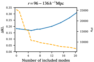
We rank the modes by how frequently they appear, then add them in that order to the projection operator. Each time we add a new mode, we perform a new round of Monte Carlo cross-validation to determine the KL divergence between the new model (with smoothed residual) and the sample covariance. The results for the low-$r$ and high-$r$ ranges are shown in Figure 2. In order to better illustrate the improvement in the KL divergence, we have subtracted off the expected KL divergence between the model (without residual) and the sample covariance of 500 draws with that model covariance.

Figure 2: Improvement in the KL divergence between the sample covariance (computed with mocks) and the model covariance (including a smoothed residual) vs. the number of modes included in the projection operator for the smoothed residual. The dashed line indicates the noise level in terms of $n_{\text{eff}}$, an effective number of mocks. In the low-$r$ range we expect a significant bias in the model (without residual), and observe a dramatic improvement by adding a modest number of modes. In the high-$r$ range the model (without residual) performs well, and adding the smoothed residual leads to negligible improvements. The increase in $\Delta\text{KL}$ as the number of modes grows occurs because the projection operator admits an increasing amount of noise to the smoothed residual.

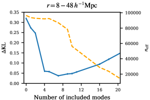
For the low-$r$ range we observe a dramatic improvement in the KL divergence using a projection operator with four modes, and modest further improvement from including seven modes. This is a clear indication that the smoothed residual brings the model closer to the true covariance matrix for the mocks. Beyond that, adding additional modes increases the KL divergence, as the projection operator admits more noise to the smoothed residual (or, equivalently, smooths less aggressively). Adding the smoothed residual extends the validity of the model covariance to low scales where it was previously unusable, and is the primary result of this note.

For the high-$r$ range we observe only modest improvement in the KL divergence. This is consistent with our expectation that the model (without residual) is quite accurate at these scales. As the number of modes increases, we see the same increase in the KL divergence that we observed for the low-$r$ range.

As an auxiliary measure of the new model we also compute the effective number of mocks, $n_{\text{eff}}$, as defined in [15]. This quantifies the noise on the covariance matrix. The original model is generated through numerical integration, so it is not noiseless. As we add more modes to the smoothed residual, we expect the noise to increase, and that consequently $n_{\text{eff}}$ should decrease. $n_{\text{eff}}$ assumes that the noise on the covariance matrix is Wishart, which is definitely not true for our model with or without the smoothed residual, so we are less interested in exact numbers and more interested in large changes. For the low-$r$ range Figure 2 shows that we can add 4-9 modes without significantly increasing the level of noise in the covariance matrix. For the high-$r$ range we find that the noise increases significantly when any modes are added.

We would like to make a sharp statement about the optimal number of modes to include in the projection operator in each case. However, as discussed above, the Monte Carlo cross-validation we have undertaken reduces, but does not eliminate, overfitting. In the low-$r$ case the mode frequencies shown in Figure 1 provide strong evidence that four modes should be included in the projection operator, with those modes appearing in almost every Monte Carlo run. The next three modes appear a little more than half the time, so the evidence in their favor is weaker. When we look at the impact of these modes on the KL divergence in Figure 2, the bulk of the improvement is dues to the initial four modes, but the KL divergence does decrease when the next three modes are included. In Figure 3 we plot the actual residual and, for comparison, the smoothed residuals with four modes and with seven modes. When four modes are included the resulting residual is quite smooth. With seven modes a sharp feature appears in the $r=8-12\,h^{-1}\text{Mpc}$ range, and it is plausible that this feature is a result of noise, not signal. We believe that the best interpretation is that the additional three modes constitute overfitting, but a more rigorous statistical analysis would be required to prove that this is the case.

Figure 3: The unsmoothed covariance matrix residual for the low-$r$ range, along with two smoothed residuals using different numbers of modes. Entries $C_{ab}$ are whitened by a factor of $r_{a}r_{b}$ to remove the leading $r$-dependence. Bins are grouped according to their $r$ values, and within each group $\mu$ values increase from $0.05$ to $0.95$. Both smoothed residuals are credible corrections to the model covariance matrix, but the question of which is preferred is difficult. Seven modes leads to the smallest KL divergence, but sharp features in the $r=8-12\,h^{-1}\text{Mpc}$ are strongly reminiscent of noise.

In the high-$r$ case the question is “should we include a smoothed residual at all?” Figure 2 shows a decrease in the KL divergence with five modes included, but the decrease is quite modest – smaller than the decrease in the low-$r$ case when increasing from four to seven modes. If we look at the mode frequencies in Figure 1, we see that the five modes we might include occurred less frequently than the three modes we found spurious in the low-$r$ case. Finally, in Figure 4 we plot the actual residual and smoothed residual, and observe no structure of note in the smoothed residual. We conclude that the drop in KL divergence shown in Figure 2 is a result of overfitting, and that for high $r$ the model should be used without a smoothed residual.

Figure 4: The unsmoothed covariance matrix residual for the low-$r$ range, along with the smoothed residual using five modes. Entries $C_{ab}$ are whitened by a factor of $r_{a}r_{b}$ to remove the leading $r$-dependence. Although the unsmoothed residual appears to exhibit structure, it has not survived cross-validation and we conclude that it is noise. The smoothed residual is close to zero – note the different scales for the two plots.

5 Discussion

We have introduced a method for combining a model covariance matrix with a set of mocks. The resulting covariance matrix can incorporate features of the mocks that were not reflected in the model, while maintaining low levels of noise. To demonstrate the method we constructed a covariance matrix for a BOSS-like survey that would be applicable at separations of $8-40\,h^{-1}\text{Mpc}$, scales where a Gaussian model covariance matrix would not be valid. While this represents valuable progress in covariance matrix estimation, we briefly discuss two limitations of the method.

The smoothed residual approach rests on our ability to select eigenvectors of the model covariance matrix which efficiently describe the difference between the model and mock covariance matrices. As discussed in the text, our method appears to select a few more modes than would be optimal. Our use of cross-validation reduces this overfitting, but does not eliminate it entirely. Further statistical work might reveal an approach that corrects this.

A second limitation is that we assume that the mock covariance matrix is not biased, relative to the true covariance matrix for the survey. This is a strong assumption, and one that could be violated in a meaningful way in practical applications. We recently demonstrated that models of non-Gaussianity can be calibrated directly against the survey using jackknife techniques [19], but the approach introduced here does not include a model for the residual and so cannot be connected to the survey in this way. The accuracy of the mocks used is therefore a limiting factor.

References

- Taylor and Joachimi [2014] Andy Taylor and Benjamin Joachimi. Estimating Cosmological Parameter Covariance. Monthly Notices of the Royal Astronomical Society, 442(3):2728–2738, 2014, 1402.6983.
- Dodelson and Schneider [2013] Scott Dodelson and Michael D. Schneider. The Effect of Covariance Estimator Error on Cosmological Parameter Constraints. Phys.Rev., D88:063537, 2013, 1304.2593.
- Percival et al. [2014] Will J. Percival et al. The Clustering of Galaxies in the SDSS-III Baryon Oscillation Spectroscopic Survey: Including covariance matrix errors. Monthly Notices of the Royal Astronomical Society, 439(3):2531–2541, 2014, 1312.4841.
- Zhu et al. [2015] Fangzhou Zhu, Nikhil Padmanabhan, and Martin White. Optimal Redshift Weighting For Baryon Acoustic Oscillations. Monthly Notices of the Royal Astronomical Society, 451:4755, 2015, 1411.1424.
- Padmanabhan et al. [2016] Nikhil Padmanabhan, Martin White, Harrison H. Zhou, and Ross O’Connell. Estimating sparse precision matrices. Mon. Not. Roy. Astron. Soc., 460(2):1567–1576, 2016, 1512.01241.
- Escoffier et al. [2016] S. Escoffier, M. C. Cousinou, A. Tilquin, A. Pisani, A. Aguichine, S. de la Torre, A. Ealet, W. Gillard, and E. Jullo. Jackknife resampling technique on mocks: an alternative method for covariance matrix estimation. ArXiv e-prints, 2016, 1606.00233.
- Joachimi [2017] Benjamin Joachimi. Non-linear shrinkage estimation of large-scale structure covariance. Mon. Not. Roy. Astron. Soc., 466:L83, 2017, 1612.00752.
- Klypin and Prada [2018] Anatoly Klypin and Francisco Prada. Dark matter statistics for large galaxy catalogues: power spectra and covariance matrices. Monthly Notices of the Royal Astronomical Society, 478(4):4602–4621, 2018, 1701.05690.
- Howlett and Percival [2017] Cullan Howlett and Will J. Percival. Galaxy two-point covariance matrix estimation for next generation surveys. Mon. Not. Roy. Astron. Soc., 472(4):4935–4952, 2017, 1709.03057.
- Zhu et al. [2018] Fangzhou Zhu et al. The clustering of the SDSS-IV extended Baryon Oscillation Spectroscopic Survey DR14 quasar sample: measuring the anisotropic baryon acoustic oscillations with redshift weights. Mon. Not. Roy. Astron. Soc., 480(1):1096–1105, 2018, 1801.03038.
- Barreira et al. [2018] Alexandre Barreira, Elisabeth Krause, and Fabian Schmidt. Accurate cosmic shear errors: do we need ensembles of simulations? JCAP, 1810(10):053, 2018, 1807.04266.
- Wang et al. [2019] Yuting Wang, Gong-Bo Zhao, and John A. Peacock. Extracting key information from spectroscopic galaxy surveys. 2019, 1910.09533.
- Philcox et al. [2019] Oliver H. E. Philcox, Daniel J. Eisenstein, Ross O’Connell, and Alexander Wiegand. RascalC: A Jackknife Approach to Estimating Single and Multi-Tracer Galaxy Covariance Matrices. 2019, 1904.11070.
- Philcox and Eisenstein [2019] Oliver H. E. Philcox and Daniel J. Eisenstein. Estimating Covariance Matrices for Two- and Three-Point Correlation Function Moments in Arbitrary Survey Geometries. 2019, 1910.04764.
- O’Connell et al. [2016] Ross O’Connell, Daniel Eisenstein, Mariana Vargas, Shirley Ho, and Nikhil Padmanabhan. Large covariance matrices: smooth models from the two-point correlation function. Mon. Not. Roy. Astron. Soc., 462(3):2681–2694, 2016, 1510.01740.
- Kullback [1951] R. A. Kullback, S.; Leibler. On information and sufficiency. Ann. Math. Statist., 22(1):79–86, 1951.
- White et al. [2014] Martin White, Jeremy L. Tinker, and Cameron K. McBride. Mock galaxy catalogues using the quick particle mesh method. Monthly Notices of the Royal Astronomical Society, 437(3):2594–2606, 2014, 1309.5532.
- Dawson et al. [2013] K. S. Dawson, D. J. Schlegel, C. P. Ahn, S. F. Anderson, É. Aubourg, S. Bailey, R. H. Barkhouser, J. E. Bautista, A. Beifiori, A. A. Berlind, V. Bhardwaj, D. Bizyaev, C. H. Blake, M. R. Blanton, M. Blomqvist, A. S. Bolton, A. Borde, J. Bovy, W. N. Brandt, H. Brewington, J. Brinkmann, P. J. Brown, J. R. Brownstein, K. Bundy, N. G. Busca, W. Carithers, A. R. Carnero, M. A. Carr, Y. Chen, J. Comparat, N. Connolly, F. Cope, R. A. C. Croft, A. J. Cuesta, L. N. da Costa, J. R. A. Davenport, T. Delubac, R. de Putter, S. Dhital, A. Ealet, G. L. Ebelke, D. J. Eisenstein, S. Escoffier, X. Fan, N. Filiz Ak, H. Finley, A. Font-Ribera, R. Génova-Santos, J. E. Gunn, H. Guo, D. Haggard, P. B. Hall, J.-C. Hamilton, B. Harris, D. W. Harris, S. Ho, D. W. Hogg, D. Holder, K. Honscheid, J. Huehnerhoff, B. Jordan, W. P. Jordan, G. Kauffmann, E. A. Kazin, D. Kirkby, M. A. Klaene, J.-P. Kneib, J.-M. Le Goff, K.-G. Lee, D. C. Long, C. P. Loomis, B. Lundgren, R. H. Lupton, M. A. G. Maia, M. Makler, E. Malanushenko, V. Malanushenko, R. Mandelbaum, M. Manera, C. Maraston, D. Margala, K. L. Masters, C. K. McBride, P. McDonald, I. D. McGreer, R. G. McMahon, O. Mena, J. Miralda-Escudé, A. D. Montero-Dorta, F. Montesano, D. Muna, A. D. Myers, T. Naugle, R. C. Nichol, P. Noterdaeme, S. E. Nuza, M. D. Olmstead, A. Oravetz, D. J. Oravetz, R. Owen, N. Padmanabhan, N. Palanque-Delabrouille, K. Pan, J. K. Parejko, I. Pâris, W. J. Percival, I. Pérez-Fournon, I. Pérez-Ràfols, P. Petitjean, R. Pfaffenberger, J. Pforr, M. M. Pieri, F. Prada, A. M. Price-Whelan, M. J. Raddick, R. Rebolo, J. Rich, G. T. Richards, C. M. Rockosi, N. A. Roe, A. J. Ross, N. P. Ross, G. Rossi, J. A. Rubiño-Martin, L. Samushia, A. G. Sánchez, C. Sayres, S. J. Schmidt, D. P. Schneider, C. G. Scóccola, H.-J. Seo, A. Shelden, E. Sheldon, Y. Shen, Y. Shu, A. Slosar, S. A. Smee, S. A. Snedden, F. Stauffer, O. Steele, M. A. Strauss, A. Streblyanska, N. Suzuki, M. E. C. Swanson, T. Tal, M. Tanaka, D. Thomas, J. L. Tinker, R. Tojeiro, C. A. Tremonti, M. Vargas Magaña, L. Verde, M. Viel, D. A. Wake, M. Watson, B. A. Weaver, D. H. Weinberg, B. J. Weiner, A. A. West, M. White, W. M. Wood-Vasey, C. Yeche, I. Zehavi, G.-B. Zhao, and Z. Zheng. The Baryon Oscillation Spectroscopic Survey of SDSS-III. Astrophysical Journal, 145:10, January 2013, 1208.0022.
- O’Connell and Eisenstein [2018] Ross O’Connell and Daniel J. Eisenstein. Large Covariance Matrices: Accurate Models Without Mocks. 2018, 1808.05978.