NLO impact factor for inclusive photon$+$dijet production in $e+A$ DIS at small $x$

Abstract

We compute the next-to-leading order (NLO) impact factor for inclusive photon $+$dijet production in electron-nucleus (e+A) deeply inelastic scattering (DIS) at small $x$. An important ingredient in our computation is the simple structure of “shock wave” fermion and gluon propagators. This allows one to employ standard momentum space Feynman diagram techniques for higher order computations in the Regge limit of fixed $Q^{2}\gg\Lambda_{\rm QCD}^{2}$ and $x\rightarrow 0$. Our computations in the Color Glass Condensate (CGC) effective field theory include the resummation of all-twist power corrections $Q_{s}^{2}/Q^{2}$, where $Q_{s}$ is the saturation scale in the nucleus. We discuss the structure of ultraviolet, collinear and soft divergences in the CGC, and extract the leading logs in $x$; the structure of the corresponding rapidity divergences gives a nontrivial first principles derivation of the JIMWLK renormalization group evolution equation for multiparton lightlike Wilson line correlators. Explicit expressions are given for the $x$-independent $O(\alpha_{s})$ contributions that constitute the NLO impact factor. These results, combined with extant results on NLO JIMWLK evolution, provide the ingredients to compute the inclusive photon $+$ dijet cross-section at small $x$ to $O(\alpha_{s}^{3}\ln(x))$. First results for the NLO impact factor in inclusive dijet production are recovered in the soft photon limit. A byproduct of our computation is the LO photon+ 3 jet (quark-antiquark-gluon) cross-section.

I Introduction

An important discovery of the electron-proton ($e+p$) deep inelastic scattering (DIS) experiments at HERA was the rapid growth of the gluon distribution with decreasing Bjorken $x$, for fixed large momentum transfer squared $Q^{2}$. This demonstrated that the proton wavefunction in the corresponding high energy Regge limit is dominated by Fock state configurations containing large numbers of gluons. Their number grows via bremsstrahlung with increasing energy or decreasing $x$. It was conjectured that in this Regge limit repulsive gluon recombination and screening effects Gribov:1984tu; Mueller:1985wy conspire to slow down the growth of cross-sections. A remarkable consequence is that a semi-hard saturation scale $Q_{s}(x)$ is generated dynamically by these competing many-body effects.

If the saturation scale is large compared to the intrinsic QCD scale, asymptotic freedom suggests that the coupling $\alpha_{s}(Q_{s})\ll 1$; this allows weak coupling effective field theory techniques to be employed in systematically computing cross-sections in a regime of QCD where field strengths are nonperturbatively large. The physics of this nonlinear regime of QCD can be quantified in a classical effective field theory (EFT) called the Color Glass Condensate (CGC) McLerran:1993ni; McLerran:1993ka; McLerran:1994vd; Iancu:2003xm; Gelis:2010nm; Kovchegov:2012mbw; Blaizot:2016qgz which implements a Born-Oppenheimer separation of the relevant degrees of freedom into static color sources at large $x$ and gauge fields at small $x$.

A further important element in the EFT is that the separation in $x$ between color sources and fields satisfies a renormalization group (RG) equation as the scale separation is evolved towards smaller $x$. This can be understood in a Wilsonian picture wherein, with each small change $\delta x$ in the scale separation, the dynamical gauge degrees of freedom within $\delta x$ are absorbed into the static light cone color sources in the classical EFT at the lower $x-\delta x$ scale. The RG equation correspondingly describes the change in a nonperturbative weight functional describing the distribution of color sources, from large $x$ towards smaller $x$, and efficiently resums simultaneously logarithms in $\alpha_{s}\ln(1/x)$ and power corrections $Q_{s}^{2}(x)/Q^{2}$ when they become large. To leading logarithmic accuracy in $x$, this RG equation is the JIMWLK equation JalilianMarian:1997gr; JalilianMarian:1997dw; Iancu:2000hn; Ferreiro:2001qy with a corresponding JIMWLK Hamiltonian Weigert:2000gi that contains all the relevant information regarding the rapidity evolution of n-point Wilson line correlators.

A number of well-known results are obtained as limits of the JIMWLK Hamiltonian. In the limit of large number of colors $N_{c}$, and for large atomic nuclei with $A\gg 1$, the JIMWLK equation for the simplest “dipole” correlator of light-like Wilson lines describing fully inclusive DIS is the Balitsky-Kovchegov (BK) equation Balitsky:1995ub; Kovchegov:1999yj. In the leading twist limit, where $Q_{s}^{2}(x)/Q^{2}\ll 1$, this reduces to the BFKL equation Kuraev:1977fs; Balitsky:1978ic. The latter was first derived by explicit computation of perturbative QCD Feynman diagrams in Regge asymptotics.

The CGC EFT has been applied to compute a large number of final states in both DIS and in hadron-hadron collisions. An excellent introductory review of the formalism and applications can be found in Blaizot:2016qgz. An important test of the framework will be its ability to make predictions of high accuracy that can be compared to experiment. The ideal experimental conditions for such tests require access to large $Q^{2}$ and small $x$. Further, since the saturation scale is enhanced in nuclei as $Q_{s,A}^{2}\sim A^{1/3}\,Q_{s,{\rm proton}}^{2}$ Gribov:1984tu; McLerran:1993ni; Kovchegov:2012mbw , heavy nuclear targets are preferred. In principle, these conditions are achieved in proton-nucleus ($p+A$) collisions at the LHC. However large final state interactions may be present in these experiments that will complicate interpretations of the data Dusling:2018hsg. These considerations provide a major motivation for future Electron-Ion Collider (EIC) experiments Accardi:2012qut; AbelleiraFernandez:2012cc; Aschenauer:2017jsk.

Such experiments at an EIC are envisaged to have much higher luminosities than were available at HERA; this, in combination with the nuclear beams, greatly enhances the possibility that DIS $e+A$ collider measurements may uncover definitive evidence for gluon saturation. These precision DIS experiments demand higher order computations in Regge asymptotics in close analogy to how higher order computations in the Bjorken limit provided powerful tests of perturbative QCD. To further the analogy, just as one computes universal splitting functions and process dependent coefficient functions in the Bjorken limit of DIS, one needs to compute both universal multiparton lightlike correlators (or equivalently, as we shall discuss, their generating weight functional describing color charge distributions) and process dependent impact factors to higher order accuracy in the Regge limit.

The next-to-leading order (NLO) computation of the BFKL kernel has now been available for over twenty years Fadin:1998py; Ciafaloni:1998gs. Subtleties in the treatment of singularities in the NLO BFKL kernel were noticed shortly after Salam:1998tj; Ciafaloni:1999yw–for a recent comprehensive discussion, see Ducloue:2019ezk. Computations of higher order corrections to the BK equations followed in short order Balitsky:2008zza; Kovchegov:2006vj; Braun:2007vi and specific prescriptions for the running coupling following from these studies were implemented Albacete:2007yr in phenomenological studies. More recently, NLO computations of multi-point Wilson line correlators, or equivalently, the NLO JIMWLK Hamiltonian have become available Balitsky:2013fea; Kovner:2013ona; Balitsky:2014mca; Lublinsky:2016meo; Caron-Huot:2013fea and next-to-next-to-leading order (NNLO) computations of BK and JIMWLK are underway Caron-Huot:2016tzz; Caron-Huot:2017fxr.

Because of the absence of final state interactions, isolated photons are clean probes of this strongly correlated gluonic matter. Several computations Gelis:2002ki; Benic:2016yqt; Benic:2016uku; Benic:2018hvb; Altinoluk:2018uax of inclusive photon production have been performed in the CGC framework in the context of proton-nucleus ($p+A$) collisions. In a recent paper Roy:2018jxq, henceforth referred to as Paper I, we reported on a first CGC computation of the leading order differential cross-section for inclusive prompt photon production in conjunction with two jets in electron-nucleus ($e+A$) DIS at small $x$. This process has clean initial and final states and is the simplest non-trivial process besides fully inclusive DIS to study the physics of gluon saturation in $e+A$ collisions. This computation provides more differential phase space distributions, thereby going beyond existing small $x$ computations Bartels:2000gt; Bartels:2002uz; Bartels:2001mv; Balitsky:2010ze; Balitsky:2012bs; Beuf:2011xd; Beuf:2016wdz; Beuf:2017bpd; Hanninen:2017ddy on the total cross-section for fully inclusive DIS; exceptions are the NLO differential cross-section computations by Boussarie et al. Boussarie:2014lxa; Boussarie:2016ogo; Boussarie:2016bkq, albeit for diffractive DIS.

In Paper I, we showed explicitly how in the limit of the final state photon momentum $k_{\gamma}\rightarrow 0$, the Low-Burnett-Kroll soft photon theorem Low:1958sn; Burnett:1967km; Bell:1969yw allows one to recover existing results for inclusive dijet production in DIS Dominguez:2011wm. In the leading twist limit, we also obtained the $k_{\perp}$ and collinear factorized expressions which match the dominant NLO small $x$ perturbative QCD (pQCD) contributions. In particular, our result in the collinear limit is directly proportional to the nuclear gluon distribution at small $x$.

For precision physics in pQCD, it is essential to go beyond leading order descriptions for quantitative studies of data. NLO computations will be especially important for the discovery and characterization of gluon saturation in $e+A$ DIS where its effects are anticipated to be larger than in $e+p$ DIS. As we observed in our LO photon+dijet computation, there are novel quadrupole gauge invariant correlators of lightlike Wilson lines that appear, whose energy evolution, in addition to the dipole correlators measured in fully inclusive DIS, will be a sensitive test of JIMWLK evolution. We will show how such correlators, in combination with the dipole correlators, violate the soft gluon theorem. A quantitative understanding of this violation can provide deeper insight into the infrared structure of QCD in the Regge limit Strominger:2017zoo.

Byproducts of our computation of the differential photon+dijet cross-section are the first NLO results for inclusive dijet, inclusive photon and photon+jet measurements at an EIC. Further, the NLO graphs for real gluon emission provide the complete LO results for the photon+3-jet ($\gamma+q\bar{q}g$) and 3-jet $q\bar{q}g$ final states Ayala:2016lhd. We will point to the steps necessary for extracting “numbers” from our computation; though much more computationally challenging than comparable computations in the highly developed collinear factorization pQCD framework, such a program is feasible and essential for precision physics at an EIC.

As we will discuss further shortly, all computations in the CGC EFT rely on a separation of scales between static color sources and dynamical gauge fields. Thus perturbative computations at small $x$ in this framework are performed in a background of such static color sources and physical quantities are obtained by subsequent gauge invariant averaging over these sources. The first principles formalism in quantum field theory underlying such computations in strong background fields has been discussed previously Gelis:2006yv; Gelis:2006cr; Gelis:2007kn; Gelis:2008rw; Jeon:2013zga; in particular, Gelis:2006yv and Jeon:2013zga provide pedagogical discussions in complementary approaches.

We begin our discussion of the NLO DIS photon+dijet computation with the starting point of all CGC computations, the classical Yang-Mills equations,

$$[D_{\mu},F^{\mu\nu}](x)=g\,\delta^{\nu+}\delta(x^{-})\rho_{A}(\bm{x}_{\perp})\,.$$ (1)

Here the covariant derivative $D_{\mu}=\partial_{\mu}-igA_{\mu}$, $g$ represents the QCD gauge coupling, and $\rho_{A}(x^{-},\bm{x}_{\perp})\approx\rho_{A}(\bm{x}_{\perp})\delta(x^{-})$ represents the color charge density of large $x$ static sources for the small $x$ dynamical fields $A^{\mu}$. The delta-function in the color charge density denotes that we are working in a frame where the nucleus is moving in the positive $z$-direction at nearly the speed of light with large light cone longitudinal momentum $P^{+}_{N}\rightarrow\infty$. (See Appendix LABEL:sec:conventions for details of the conventions adopted in this work.) In addition we will choose the frame in which the virtual photon has a large longitudinal momentum $q^{-}$ and transverse momentum $\bm{q}_{\perp}=0$.

The solution of the classical equations in Lorenz gauge $\partial_{\mu}A^{\mu}=0$ is given by

$$A_{\rm cl}^{+}=\int\frac{\mathrm{d}^{2}\bm{z}_{\perp}}{4\pi}\,\ln\frac{1}{(\bm{x}_{\perp}-\bm{z}_{\perp})^{2}\Lambda^{2}}\,\rho_{A}(x^{-},\bm{z}_{\perp})\,\,;\,\,A_{\rm cl}^{-}=0\,\,;\,\,A_{{\rm cl},\perp}=0\,,$$ (2)

where $\Lambda$ is an infrared cutoff that is necessary to invert the Laplace equation $-\nabla_{\perp}^{2}A_{\rm cl}^{+}=g\rho_{A}$ in two dimensions. This solution to the Yang-Mills equations in Lorenz gauge is simply related to the solution in the light cone gauge ${\tilde{A}}^{+}=0$, where one obtains likewise that ${\tilde{A}}_{\rm cl}^{-}=0$ and ${\tilde{A}}_{\rm cl}^{i}=\frac{i}{g}U\partial^{i}U^{\dagger}$, and

$$U(\bm{x}_{\perp})=P_{-}\Bigg{(}\text{exp}\Bigg{\{}-ig\int_{-\infty}^{+\infty}\mathrm{d}z^{-}A_{\rm cl}^{+,a}(z^{-},\bm{x}_{\perp})\,T^{a}\Bigg{\}}\Bigg{)}\,,$$ (3)

denotes the adjoint Wilson line expressed in terms of the the large $x$ static color source densities via Eq. (2). Note that $T^{a}$, $a=1,\cdots,8$ are the generators of color $SU(3)$ in the adjoint representation.

These Wilson lines, and their counterparts ${\tilde{U}}$ in the fundamental representation represent respectively, the path ordered phase acquired by a gluon and a quark in their eikonal multiple scattering off the classical background field of a nucleus. The Wilson line ${\tilde{U}}$ is obtained by replacing the adjoint generators in Eq. (3) with the fundamental generators: $T^{a}\rightarrow t^{a}$. In the LO photon+dijet cross-section of Paper I, the virtual photon fluctuates into a quark-antiquark pair that multiple scatters off the classical background field of the nucleus. In the Feynman diagram computations of this LO process, the Wilson lines are incorporated in the momentum space structure of the dressed quark propagators. At NLO, there are real and virtual gluon contributions to the leading order process. The corresponding gluon propagators are also dressed by multiple scattering off the classical background field of the nucleus.

The structure of the dressed quark and gluon propagators in the classical background field, is particularly simple in the “wrong” light cone (LC) gauge $A^{-}=0$. As indicated by Eq. (2), this gauge shares the same classical field solution with Lorenz gauge. However, unlike the LC gauge $A^{+}=0$ for $P^{+}_{N}\rightarrow\infty$, it does not provide a simple physical interpretation of parton distribution functions. Any concern in this regard is however far outweighed by the advantages provided by the simple forms of the dressed propagators that were computed previously in Refs. McLerran:1994vd; Ayala:1995hx; Ayala:1995kg; Balitsky:1995ub; McLerran:1998nk; Balitsky:2001mr. The effective vertices for these dressed quark and gluon “shockwave” propagators, incorporating the fundamental and adjoint Wilson lines respectively, are shown in Fig. 1.

As discussed in Paper I, these effective vertices are identical to the quark-quark-reggeon and gluon-gluon-reggeon effective vertices Caron-Huot:2013fea; Bondarenko:2017vfc; Ayala:2017rmh; Hentschinski:2018rrf; Bondarenko:2018kqs; Bondarenko:2018eid in Lipatov’s reggeon field theory Lipatov:1996ts. Another salient feature in the expressions below is that we do not subtract the unit matrix in the expansion of Wilson lines. This allows for the possibility that the quarks and gluons do not scatter in addition to all their possible multiple scatterings encoded in the higher terms in the Wilson line expansion. Consequently, we draw Feynman diagrams with all dressed fermion and gluon propagators and for each such kinematically allowed process, we only need to subtract the “no scattering” contribution (obtained by putting $\tilde{U}$ and $U$’s to unity) to get the physical amplitude. As we will see, this significantly aids in the NLO computation where the number of contributing processes is large.

Note further that since our computations do not employ light-front perturbation theory like many of the NLO computations in the literature, and are carried out entirely in momentum space (also unlike many computations), they also provide a useful cross-check on extant NLO results on fully inclusive DIS. The techniques employed here may also provide a pathway to carrying out higher order computations to NNLO in the Regge limit.

Figure 1: Feynman diagrams for the dressed quark and gluon propagators with effective vertices denoted respectively by crossed and filled blobs. The respective effective vertices are also shown. $i$ and $j$ represent color indices in the fundamental representation of $SU(N_{c})$ whereas $a$ and $b$ stand for the same in the adjoint representation. In the saturation regime these vertices are effectively of order unity.

To proceed with our NLO computation, it is important to elaborate further on the RG procedure for resummation of large logarithms in $x$, specifically with regard to how it applies to the inclusive photon+dijet computation of interest. As noted, the Wilsonian RG ideology on which the CGC EFT is based naturally involves a cutoff scale in rapidity or longitudinal momentum separating the soft and hard partons in a hadron/nucleus. At LO, this scale $\Lambda_{0}^{+}$ (or rapidity $Y_{0}=\ln(\Lambda_{beam}^{+}/\Lambda_{0}^{+})$) is arbitrary and the fast or valence modes with longitudinal momenta $k^{+}\gg\Lambda_{0}^{+}$ are represented by the stochastic color charge density, $\rho_{A}(x^{-},\bm{x}_{\perp})$. A gauge invariant weight functional $W_{\Lambda_{0}^{+}(Y_{0})}[\rho_{A}]$ describes the probability density corresponding to this charge density. As also noted, the soft modes are represented by classical color fields that are solutions of the classical Yang-Mills equations with appropriate gauge fixing conditions.

As we boost the nucleus towards the small $x$ scale of interest (or towards higher energies), modes that were below the cutoff $\Lambda_{0}^{+}$ start contributing to the scattering process. We therefore have to consider quantum effects induced by these “semi-fast” gluons Iancu:2000hn (see Fig. 2) which can be defined as the nearly on-shell fluctuations with momenta deeply inside the strip $\Lambda_{1}^{+}(=b\Lambda^{+}_{0})\ll|l^{+}|\ll\Lambda_{0}^{+}$ or conversely, energies in the range $\Lambda_{0}^{-}\ll|l^{-}|\ll\Lambda^{-}_{0}/b$ where

$$\Lambda^{-}_{0}=\frac{Q^{2}_{0}}{2x_{0}P^{+}_{N}}=\frac{Q^{2}_{0}}{x_{0}}.\frac{x}{Q^{2}}q^{-}\,.$$ (4)

Here $Q^{2}_{0}$ and $x_{0}$ are respectively the virtuality of the nucleus and the Bjorken-$x$ at the initial scale. Further, $Q^{2}=-2q^{+}q^{-}$ is the fixed virtuality of the exchanged virtual photon in DIS (in Regge kinematics) and $x$ is the Bjorken-$x$ of interest determined by the kinematics of the process. The effect of integrating out these fluctuations manifests itself in the appearance of large logarithms $\ln(1/b)$ which for $\alpha_{S}\ln(1/b)\sim 1$ must be resummed to all orders in $\alpha_{S}$.

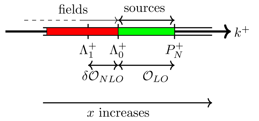
Figure 2: Schematic illustration of sources and fields in the CGC effective theory in terms of the cutoff scale $\Lambda_{0}^{+}$, or equivalently the rapidity $Y_{0}$. At NLO, contributions from field modes in the range $\Lambda_{1}^{+}<k^{+}<\Lambda_{0}^{+}$, such that $\alpha_{S}\ln(\Lambda_{0}^{+}/\Lambda_{1}^{+})\equiv\alpha_{S}\Delta Y<1$, are integrated out and absorbed into the source densities at the scale $\Lambda_{1}^{+}$. This self-similar renormalization group (RG) pattern is repeated successively generating the JIMWLK RG equation for the source densities.

Denoting the differential cross-section for inclusive photon plus dijet production by $\mathrm{d}\sigma$ for simplicity, we can write down its expectation value in the CGC EFT at LO as Roy:2018jxq

$$\langle\mathrm{d}\sigma_{\text{LO}}\rangle=\int[\mathcal{D}\rho_{A}]\,W_{\Lambda_{0}^{-}}[\rho_{A}]\,\mathrm{d}\hat{\sigma}_{\text{LO}}[\rho_{A}]\,.$$ (5)

The r.h.s represents the fact that the LO cross-section is first computed for a fixed distribution of color sources $\rho_{A}$ with $\Lambda^{-}<\Lambda_{0}^{-}$. This object $\mathrm{d}\hat{\sigma}_{\text{LO}}[\rho_{A}]$ shown in Fig. 3, is computed using standard techniques in perturbative QCD albeit, as noted, with the modified propagators listed in Fig. 1, wherein the dependence on $\rho_{A}$ enters (at LO) via the fundamental Wilson line ${\tilde{U}}$.

Figure 3: Processes contributing to the leading order amplitude and hence the cross-section $\mathrm{d}\hat{\sigma}_{\rm LO}$ in Eq. 5. The other two diagrams are obtained simply by interchanging the quark and antiquark lines.

The process independent weight functional $W_{\Lambda_{0}^{-}}[\rho_{A}]$ is a nonperturbative object that contains fundamental information about $n$-body correlations amongst gluons at the initial scale $\Lambda_{0}^{-}$. It can be understood as representing large $x$ diagonal elements of the density matrix of QCD in the Regge limit; a recent discussion of $W[\rho_{A}]$, and generalizations thereof, can be found in Armesto:2019mna.

Figure 4: NLO contributions from gluon modes with $l^{-}<\Lambda^{-}_{0}$ fluctuating within the target. The dashed horizontal line represents the EFT scale $\Lambda_{0}^{-}$ separating the gluon modes in the target and the projectile dipole. The diagrams shown are representative of those containing the large logarithms $\ln(\Lambda_{1}^{-}/\Lambda_{0}^{-})$ that contribute towards the LL$x$ evolution of $W[\rho_{A}]$.

At NLO ($\equiv O(\alpha_{S})$) in the CGC power counting, we have to account for quantum fluctuations of both the quark-antiquark dipole as well as the wavefunction of the nuclear target. In the EFT language, these are distinguished by the magnitude of the LC momentum of the gluon modes relative to the initial scale $\Lambda_{0}^{-}$. As shown in Fig. 4, the modes with $l^{-}<\Lambda_{0}^{-}$ (which we shall denote as NLO:1) can be interpreted as contributions from Fock states dressing the target wavefunction. The contribution to the cross-section for processes of this kind can in general be written as

$$\langle\mathrm{d}\sigma_{\text{NLO}:1}\rangle=\int[\mathcal{D}\rho_{A}]\,W_{\Lambda_{0}^{-}}[\rho_{A}]\,\mathrm{d}\hat{\sigma}_{\text{NLO}:1}[\rho_{A}]\,,$$ (6)

where $\mathrm{d}\hat{\sigma}_{\text{NLO}:1}[\rho_{A}]$, for a fixed configuration of $\rho_{A}$, is comprised of nontrivial combinations of Dirac traces and Fourier transforms of color traces over products of the Wilson lines ${\tilde{U}}$ and $U$. From these contributions, we are interested in collecting only pieces that contain large logarithms in $\Lambda_{0}^{-}$. These can be written as

$$\langle\delta\sigma_{\text{NLO:1}}\rangle=\int[\mathcal{D}\rho_{A}]\,W_{\Lambda^{-}_{0}}[\rho_{A}]\ln(\Lambda^{-}_{1}/\Lambda^{-}_{0})\,\,\mathcal{H}_{\text{LO}}\,\mathrm{d}\hat{\sigma}_{\text{LO}}[\rho_{A}]\,,$$ (7)

where $\Lambda_{1}^{-}$ is the scale to which the target gluon modes are evolved. Here $\mathcal{H}_{\text{LO}}$ represents the JIMWLK Hamiltonian JalilianMarian:1997gr; JalilianMarian:1997dw; Iancu:2000hn; Ferreiro:2001qy; Weigert:2000gi; its explicit form will be discussed later in the paper. For our purposes here, it suffices to note that $\mathcal{H}_{\text{LO}}\,\mathrm{d}\hat{\sigma}_{\text{LO}}$ is of order $\alpha_{S}\,\mathrm{d}\hat{\sigma}_{LO}[\rho_{A}]$. Combining the above contribution with the LO result in Eq. (5), and using the Hermiticity of $W$ with respect to the functional integration over $\rho_{A}$, we can write the result as

$$\langle\mathrm{d}\sigma_{\text{LO}}+\delta\sigma_{\text{NLO:1}}\rangle=\int[\mathcal{D}\rho_{A}]\Big{\{}\Big{(}1+\ln(\Lambda_{1}^{-}/\Lambda_{0}^{-})\mathcal{H}_{\text{LO}}\Big{)}W_{\Lambda^{-}_{0}}[\rho_{A}]\Big{\}}\,\mathrm{d}\hat{\sigma}_{\text{LO}}[\rho_{A}]\,.$$ (8)

Further redefining

$$\Big{(}1+\ln(\Lambda_{1}^{-}/\Lambda_{0}^{-})\mathcal{H}_{\text{LO}}\Big{)}W_{\Lambda_{0}^{-}}[\rho_{A}]=W_{\Lambda_{1}^{-}}[\rho_{A}]\,,$$ (9)

and thereby absorbing the effects of the semi-fast gluons in terms of a modification of the probability distribution of the fast color sources, one obtains the leading log in $x$ JIMWLK equation

$$\frac{\partial}{\partial(\ln\Lambda^{-})}W_{\Lambda^{-}}[\rho_{A}]=\mathcal{H}_{\text{LO}}\,W_{\Lambda^{-}}[\rho_{A}]\,.$$ (10)

To derive this result, we employed the essential RG philosophy that the observable on the l.h.s of Eq. 8 must be independent of the arbitrary scale $\Lambda_{0}^{-}$ separating the static color sources $\rho_{A}$ from the dynamical gauge fields. Replacing the expression in curly brackets in Eq. (8) by the r.h.s of Eq. (9) is equivalent to summing the leading logarithmic terms $\alpha_{S}\ln(1/x)$ to all orders in perturbation theory. We will henceforth label the weight functional that satisfies Eq. (10) as $W^{LLx}[\rho_{A}]$.

One also has NLO contributions from gluon modes with $l^{-}>\Lambda_{0}^{-}$ corresponding to quantum fluctuations of the dipole projectile. As shown in Fig. 5, these include real gluon emission and virtual gluon exchange processes; the filled blobs represent the dressed gluon propagators allowing for the possibility that the gluon can scatter off the background classical field of the nucleus. We will refer to contributions from the quantum fluctuations of the projectile as NLO:2 contributions to distinguish these from the NLO:1 quantum fluctuations of the target below the scale $\Lambda_{0}^{-}$.

Figure 5: Representative NLO contributions from gluon modes in the projectile with $l^{-}>\Lambda_{0}^{-}$. Both real and virtual emission diagrams are shown. For the latter case, we have to consider interference diagrams with LO processes described in Roy:2018jxq.

As in any loop computation, the intermediate steps of our calculation will contain soft, collinear and ultraviolet (UV) singularities depending on the region of phase space of the gluon that we are integrating over. In the virtual graphs, UV divergences appear from integrals over the transverse momentum of the gluon in the loop; these are isolated using dimensional regularization in $d=2-\epsilon$ dimensions. At this NLO order of quantum fluctuations of the projectile quark-antiquark pair, all UV divergences must vanish or cancel without the necessity of renormalizing the parameters of the EFT. This is because we will work the limit of massless quarks and there is no running of the QCD coupling constant in the projectile wavefunction at this order in the CGC power counting.

The small $x$ divergences arise from integrating over the quantum fluctuations induced by “slow” or “semi-fast” gluons with ‘–’ longitudinal momenta that are small relative to the large $q^{-}$ momentum of the virtual photon. These divergences are regulated by imposing a cutoff at the initial scale, $\Lambda_{0}^{-}$ of the evolution which is defined in Eq. 4. The resulting logarithms in $\Lambda_{0}^{-}$ (or equivalently $x$) are absorbed into small $x$ renormalization group evolution of the weight functional $W[\rho_{A}]$ as shown in Eq. 10. At higher orders, it may be necessary to employ more sophisticated regularization schemes for these rapidity divergences as well Liu:2019iml.

For gluon emission diagrams, in addition to small $x$ divergences, there are also singularities that arise from the region of phase space where the unscattered gluon is soft or collinear to the quark or antiquark. In particular, there are residual collinear divergences that survive after real and virtual contributions are combined. These divergences are absorbed into the evolution of fragmentation functions. Conversely, we can regulate the phase space integration over final states by promoting partons to jets where the latter are defined using a cone algorithm Sterman:1977wj; Furman:1981kf. We will show explicitly in the limit of small jet cone size Ivanov:2012ms; Aversa:1988vb; Aversa:1989xw; Jager:2004jh that collinear divergences between real and virtual graphs cancel completely enabling the extraction of the dominant contributions towards the jet cross-section.

With all the divergences in the ($\rm NLO:2$) quantum fluctuations of the virtual photon projectile accounted for, one can write the infrared (IR) safe jet cross-section as

$$\langle\mathrm{d}\sigma_{\text{NLO}:2}^{\rm jet}\rangle=\langle\delta\sigma_{\rm NLO:2}^{\rm jet}\rangle+\int[\mathcal{D}\rho_{A}]\,W_{\Lambda_{0}^{-}}[\rho_{A}]\,\mathrm{d}\hat{\sigma}_{\text{NLO}}^{\rm jet;finite}[\rho_{A}]\,.$$ (11)

These NLO contributions (shown in Fig. 5) can be broken up into two pieces. The first piece is obtained by taking the “slow” gluon limit, $l^{-}\rightarrow 0$ and is identical ($\delta\sigma_{\rm NLO:2}^{\rm jet}=\delta\sigma_{\rm NLO:1}^{\rm jet}$) to the expression in Eq. 7 at the momentum scale $\Lambda_{0}^{-}$. We will show this explicitly later in the paper. Specifically, this matching corresponds to a first principles derivation of leading log JIMWLK evolution for a nontrivial final state of the projectile. While the NLO:2 derivation represents the slow IR limit of the projectile, the RG corresponds to matching it to quantum fluctuations at their fast scale $\Lambda_{0}^{-}$ in the target.

The second term on the r.h.s of Eq. 11 ($\mathrm{d}\hat{\sigma}_{\text{NLO}}^{\text{jet;finite}}[\rho_{A}]$) contains genuine $\alpha_{S}$ suppressed (without logs in $x$) contributions to the differential cross-section from real and virtual graphs. For the latter, it is possible to deduce analytical expressions because the divergent structures can be isolated at the level of the amplitude. In contrast, divergent structures in the real NLO contributions are manifest only at the level of the squared amplitude and obtaining analytical expressions for the finite terms is challenging. However they can be evaluated numerically using the fact that rapidity divergences can be isolated in the slow gluon limit; these can then be subtracted from the squared amplitudes (using a numerical cutoff procedure) to obtain the desired finite pieces.

Further, by replacing parton momenta in these contributions with those of jets (using a jet algorithm) gets rid of the remaining collinear divergences. The finite contributions $\mathrm{d}\hat{\sigma}_{\text{NLO}}^{\text{jet;finite}}[\rho_{A}]$ that we will compute explicitly in this paper are, in the language of Regge theory, the NLO “impact factor” corrections to the LO impact factor $\mathrm{d}\hat{\sigma}_{\rm LO}^{\rm jet}[\rho_{A}]$.

Computing this process-dependent NLO impact factor $\mathrm{d}\hat{\sigma}_{\text{NLO}}^{\text{jet;finite}}[\rho_{A}]$ for photon+dijet production is important because it allows us to go one step further in precision and consider relevant (two loop) NNLO contributions to the cross-section that have terms proportional to $\alpha_{S}^{2}\ln(\Lambda_{1}^{-}/\Lambda_{0}^{-})$. These contributions are effectively of NLO magnitude if $\alpha_{S}\ln(\Lambda_{1}^{-}/\Lambda_{0}^{-})\sim 1$. Diagrams corresponding to a two loop fluctuation of the target are shown in Fig. 6. In the class of such two loop diagrams, there are contributions of order $\alpha_{S}^{2}\ln^{2}(\Lambda_{1}^{-}/\Lambda_{0}^{-})\sim O(1)$ which are included in the leading log JIMWLK resummation, as represented by $W^{LLx}[\rho_{A}]$. There are also contributions from two-loop QCD diagrams proportional to $\alpha_{S}^{2}$ alone (without leading logs in $x$) but these are suppressed at the desired accuracy of our problem. We will consider here only those two loop contributions in Fig. 6 that contain next-to-leading logarithms in $x$ (NLL$x$) contributions to the result in Eq. 8. This in turn gives us the LO+NLL$x$ result which can be expressed in terms of a modified weight-functional as

$$\langle\mathrm{d}\sigma^{\rm jet}\rangle_{\text{LO}+\text{NLL$x$}}=\int[\mathcal{D}\rho_{A}]\,W_{\Lambda_{1}^{-}}^{NLLx}[\rho_{A}]\,\mathrm{d}\hat{\sigma}_{\rm LO}^{\rm jet}[\rho_{A}]\,,$$ (12)

where

$$W_{\Lambda_{1}^{-}}^{NLLx}[\rho_{A}]=\Big{\{}1+\ln(\Lambda_{1}^{-}/\Lambda_{0}^{-})(\mathcal{H}_{\text{LO}}+\mathcal{H}_{\text{NLO}})\Big{\}}\,W_{\Lambda_{0}^{-}}[\rho_{A}]\,,$$ (13)

and the NLO JIMWLK Hamiltonian $\mathcal{H}_{\text{NLO}}$ Balitsky:2013fea; Kovner:2013ona; Balitsky:2014mca; Lublinsky:2016meo; Caron-Huot:2013fea is of order $\alpha_{S}^{2}$.

Figure 6: NNLO diagrams that contain $\alpha_{S}$ magnitude contributions for $\alpha_{S}\text{ln}(\Lambda^{-}_{1}/\Lambda^{-}_{0})\sim 1$. These diagrams contribute to the NLO JIMWLK kernel.

Figure 7: Representative NNLO diagrams whose leading logarithmic pieces are combined with the $\alpha_{S}$ suppressed contributions to show the LL$x$ evolution of the weight functional for the large-$x$ color sources at NLO.

There are however a second class of two loop NNLO contributions of the sort shown in Fig. 7 which contain contributions that are parametrically of order $\alpha_{S}^{2}\ln(\Lambda^{-}_{1}/\Lambda_{0}^{-})$. These correspond to one loop fluctuations of both the projectile and the target. From these processes, we have to extract the LL$x$ pieces from the gluon fluctuations below the cut $\Lambda_{0}^{-}$ and match them with the O($\alpha_{S}$) NLO “impact factor” expression in Eq. 11 to obtain

$$\langle\delta\sigma_{\text{NNLO}}^{\rm jet}\rangle=\int[\mathcal{D}\rho_{A}]\,W^{LLx}[\rho_{A}]\,\mathrm{d}\hat{\sigma}_{\text{NLO}}^{\text{jet;finite}}[\rho_{A}]\,.$$ (14)

As a result of our power counting in powers of $\alpha_{S}$ and $\alpha_{S}\ln(\Lambda^{-}_{1}/\Lambda_{0}^{-}$), one can finally write the complete NLO result for the differential cross-section at NLL$x$ accuracy by combining the results in Eqs. 12 and 14 respectively as

$$\langle\mathrm{d}\sigma^{\rm jet}\rangle_{\text{NLO}+\text{NLL$x$}} =\int[\mathcal{D}\rho_{A}]\,\Big{\{}W^{NLLx}[\rho_{A}]\,\mathrm{d}\hat{\sigma}_{\text{LO}}^{\rm jet}[\rho_{A}]+W^{LLx}[\rho_{A}]\,\mathrm{d}\hat{\sigma}_{\text{NLO}}^{\rm jet;finite}[\rho_{A}]\Big{\}}$$

$$\simeq\int[\mathcal{D}\rho_{A}]\,\Big{(}W^{NLLx}[\rho_{A}]\,\Big{\{}\mathrm{d}\hat{\sigma}_{\text{LO}}^{\rm jet}[\rho_{A}]+\mathrm{d}\hat{\sigma}_{\text{NLO}}^{\text{jet;finite}}[\rho_{A}]\Big{\}}+O(\alpha_{S}^{3}\ln(\Lambda^{-}_{1}/\Lambda^{-}_{0}))\Big{)}\,.$$ (15)

As the $\simeq$ in the above equation indicates, we can go one step further by promoting the second term on the r.h.s of the first equality from $W^{LLx}\rightarrow W^{NLLx}$. This extends the scope of computation to $O(\alpha_{S}^{3}\ln(1/x))$ with the understanding that we will miss terms at that order of accuracy.

The weight functional $W^{NLLx}[\rho_{A}]$ in Eq. (13) can be obtained by adapting extant results for LO and NLO($\equiv$O($\alpha_{S}^{2}$)) JIMWLK Lublinsky:2016meo; Kovner:2013ona; Kovner:2014lca; Grabovsky:2013mba; Caron-Huot:2013fea and BK Balitsky:2008zza; Balitsky:2013fea; Kovchegov:2006vj evolution into our approach. Thus to obtain results for photon+dijet production up to $O(\alpha_{S}^{3}\ln(\Lambda^{-}_{1}/\Lambda^{-}_{0}))$ accuracy, it is sufficient to compute the NLO impact factor $\mathrm{d}\hat{\sigma}_{\text{NLO}}^{\text{jet;finite}}[\rho_{A}]$. To go beyond this level of accuracy, we would have to compute fluctuations in the projectile involving the emission of two gluons, two loop virtual gluon processes, as well as interference diagrams of the genuine NLO processes shown in Fig. 5. This will be reserved for a future project.

The rest of the paper is organized as follows. In Sec. II, we shall briefly review the essential elements of the leading order (LO) computation of Paper I Roy:2018jxq and revisit some of the key results obtained there. In Sec. III, we will outline the structure of the NLO computation, structured for convenience in two subsections. In Sec. III.1 we categorize contributions to the NLO amplitudes from real gluon emission and virtual gluon exchange diagrams in terms of their color structure. We also provide an interactive flowchart (see Fig. 17) in this subsection furnished with hyperlinks that direct the reader to the final expressions later in the text for the various components constituting the real and virtual contributions to the NLO amplitude. In Sec. III.2, we organize these contributions at the level of the squared amplitude in Table 2 in terms of common Wilson line structures. Doing so enables one to see cancellations of divergences in a transparent manner; this in turn facilitates the computation of the finite NLO impact factor in the photon+dijet inclusive cross-section.

Section IV contains a detailed computation of the amplitude for real gluon emission processes. These are discussed separately for the case when the real gluon either crosses or does not cross the nuclear “shock wave” using a representative diagram from each category. The final expression for the amplitude is given by Eq. 75. In section V, we describe in detail the computation of the amplitude for virtual gluon exchange processes; these are broadly classified into the topologies of self-energy and vertex corrections. Specifically, sections V.1 and V.2 deal with the amplitudes for self-energy graphs with dressed and free gluon propagators respectively. There are ultraviolet and rapidity singularities associated with these processes which are carefully isolated from the finite parts. For each class of diagrams, we use a representative graph to show the explicit computation. The results for the amplitudes from these processes are given respectively by Eqs. 79, 106 and LABEL:eq:amplitude-self-energy-SE3. A similar exercise is performed in sections LABEL:sec:virtual-corrections-vertex and LABEL:sec:vertex-corrections-free-gluon respectively for the vertex correction processes with dressed and free gluon propagators. The final expressions for the amplitudes are given by Eqs. LABEL:eq:amplitude-V1-generic and LABEL:eq:amplitude-V2-generic for the case of dressed gluon propagators and by Eqs. LABEL:eq:amplitude-V3-generic and LABEL:eq:amplitude-V4-generic for the case in which the gluon does not cross the shock wave.

Section LABEL:sec:jet-cross-section combines the results obtained in the earlier sections to obtain the final result for the principal goal of our study, the NLO impact factor for photon $+$ dijet production in $e+A$ DIS. We demonstrate here the cancellation of collinear divergences between real and virtual processes resulting in an infrared safe differential cross-section. To facilitate this, we introduce jet definitions and work in the approximation of a jet with small cone radius Ivanov:2012ms to explicitly extract the collinearly divergent contributions from the squared amplitudes of real gluon emission graphs which contain the possibility of a gluon being collinear to the (anti) quark. We note that there is no Sudakov suppression of the cross-section because we have not imposed any kinematic constraints. Interestingly, we observe that (unlike the case of diffractive DIS Boussarie:2016ogo) the NLO cross-section does not factorize into the LO result and kinematic factors in the soft gluon limit. The implications of this result will be addressed in future work.

In Section LABEL:sec:JIMWLK-evolution, we take the slow gluon limit of our general expressions for the cross-sections and show that these provide a first principles derivation of the JIMWLK RG equation. While there exist several derivations of the JIMWLK equation in the literature going back to the original papers, many of these begin at the outset in the slow gluon limit. It is therefore interesting to see how the JIMWLK equation arises in the explicit computation of the nontrivial photon+dijet cross-section. This exercise also helps lay the groundwork for an independent derivation of the NLL$x$ JIMWLK equation.

We will end this paper with a brief summary and outlook. With regard to the latter, an important next step is to provide quantitative predictions for measurements at a future EIC. These are significantly more challenging even though our use of the wrong light cone ($A^{-}=0$) gauge allows us to present our computations in a manner analogous to comparable NLO computations in collinear factorization computations. This is firstly because going away from the collinear limit introduces additional nontrivial integrals in the computations. Further, a quantitative computation of the dipole and quadrupole correlations is much more complex than their parton distribution (pdf) counterparts. This is unsurprising because the former contain a tremendous amount of information on the physics of many-body correlations in QCD that are not contained in the pdfs. Nevertheless, the technology to achieve the desired goal has advanced considerably to bring it within reach.

The principal results and conclusions of this paper are spelled out in an accompanying letter Roy:2019cux.

Appendices LABEL:sec:conventions through LABEL:sec:non-collinear-contributions supplement the material in the body of the paper. The notations and conventions used throughout the paper are summarized in Appendix LABEL:sec:conventions. In the computation of the amplitude for the various processes, we will encounter tensor integrals over transverse components of the gluon loop momenta. General expressions for these constituent integrals along with details for special cases are provided in Appendix LABEL:sec:constituent-integrals-real-emission for both processes with gluon emissions and gluon loops. Appendix LABEL:sec:R-factors-real-emission contains detailed expressions for the amplitudes for gluon emission processes that are too cumbersome to include in the main text. Likewise, in Appendix LABEL:sec:quark-self-energy, we provide a detailed computation of the quark self-energy, which provides the template to compute the amplitudes of self-energy graphs where the gluon propagator is not dressed. The expression obtained in Eq. LABEL:eq:quark-selfenergy-loop-contribution for the gluon loop contribution is very general and can be straightforwardly used in any pQCD computation performed using light cone coordinates and in the light cone gauge. A similar computation for the virtual gluon corrections to the $\gamma qq$ and $\gamma^{*}q\bar{q}$ vertices is provided in Appendices LABEL:sec:quark-real_photon-quark-vertex-gluon-correction and LABEL:sec:vertex-correction-computation.

Appendix LABEL:sec:T-V1-div-parts contains the rapidity divergent pieces, discussed in Sec. LABEL:sec:virtual-corrections-vertex, for the vertex corrections with the dressed gluon propagator that are not provided in the main text. Similar expressions for the amplitudes with final state interactions (discussed in Sec. LABEL:sec:vertex-corrections-free-gluon) are provided in Appendix LABEL:sec:T-V4-div-parts. The expressions for the finite pieces of the amplitudes are distributed over seven subsections in Appendix LABEL:sec:finite-pieces-virtual-graphs. Finally, Appendix LABEL:sec:non-collinear-contributions provides a short proof of the sub-dominance of non-collinearly divergent contributions to the cross-section for real gluon emissions when we work in the limit of small jet cone radius.

II General definitions and brief review of LO computation

We will work in the light cone (LC) gauge $A^{-}=0$ throughout this computation. The highly energetic nucleus is considered to be right moving so that it has a large ‘$+$’ component of LC momentum $P_{N}^{+}$. The virtual photon exchanged between the electron and nucleus is considered to be left moving and consequently has a large ‘$-$’ component of LC momentum $q^{-}$. The mass of the electron is neglected throughout the calculation.

Following the LO computation in Roy:2018jxq, we can write the amplitude for inclusive photon$+$dijet production in DIS as

$$\mathcal{M}(\bm{\tilde{l}},\bm{\tilde{l^{\prime}}},\bm{q},\bm{k},\bm{p},\bm{k}_{\gamma})=\frac{e}{Q^{2}}\overline{u}(\tilde{l^{\prime}})\,\mathcal{G}^{\mu}_{q}\,u(\tilde{l})\mathcal{M}_{\mu}(\bm{q},\bm{k},\bm{p},\bm{k}_{\gamma};\lambda)\enskip,$$ (16)

where

$$\mathcal{G}^{\mu}_{q}=\gamma^{\mu}-\frac{\not{q}n^{\mu}+q^{\mu}\gamma^{-}}{q^{-}},\qquad n^{\mu}=\delta^{\mu+}\,,$$ (17)

is obtained by index contraction with the propagator for the exchanged photon with momentum $q=(-Q^{2}/2q^{-},q^{-},\bm{0}_{\perp})$. The amplitude for the hadronic subprocess is given by

$$\mathcal{M}_{\mu}(\bm{q},\bm{k},\bm{p},\bm{k}_{\gamma};\lambda)=\epsilon^{*\alpha}(\bm{k}_{\gamma},\lambda)\mathcal{M}_{\mu\alpha}(\bm{q},\bm{k},\bm{p},\bm{k}_{\gamma})\enskip,$$ (18)

and is the quantity of interest. Here $\epsilon(\bm{k}_{\gamma},\lambda)$ is the polarization vector for the outgoing photon. The 4-momentum assignments are given in Table 1 and boldface letters denote 3-momentum vectors.

Table 1: 4-momentum assignments used in the calculation

$q$: Exchanged virtual photon	$\tilde{l}$: Incoming electron	${\tilde{l}}^{\prime}$: Outgoing electron
$k$: Quark, directed outward	$p$: Antiquark, directed outward	$k_{\gamma}$: Outgoing photon
$l_{i}$: Quark or gluon internal (loop) momentum to be integrated over	$k_{g}$: Outgoing real gluon
$P_{\text{tot}}$: Total momentum of final state in real emission= $p+k+k_{\gamma}+k_{g}$
$P$: Total momentum of final state in virtual emission and LO= $p+k+k_{\gamma}$

We define the following ratios of the outgoing momenta to the dominant component $q^{-}$ of the incoming virtual photon momentum

$$z_{q}=\frac{k^{-}}{q^{-}},\quad z_{\bar{q}}=\frac{p^{-}}{q^{-}},\quad z_{\gamma}=\frac{k^{-}_{\gamma}}{q^{-}},\quad z_{g}=\frac{k_{g}^{-}}{q^{-}}\,.$$ (19)

We will work in the limit of light quarks and neglect their masses in the present computation. Since we are dealing with prompt photon production in DIS at small $x$, the dominant contribution is indeed expected to involve light quarks.

Squaring the expression for the amplitude in Eq. (16), and performing the necessary averaging and sum over electron spins and photon polarizations, we can write

$$\frac{1}{2}\sum_{\text{spins},\lambda}|\mathcal{M}|^{2}=L^{\mu\nu}X_{\mu\nu}\enskip.$$ (20)

The lepton tensor given by

$$L^{\mu\nu}=\frac{e^{2}}{2Q^{4}}\,\text{tr}\,[\tilde{\not{l}}\mathcal{G}^{\mu}_{q}{\not{\tilde{l}}}^{\prime}\mathcal{G}^{\nu}_{q}]\,,$$ (21)

is identical to the one obtained in fully inclusive DIS.

In the following, we will concentrate on obtaining the NLO contributions to the hadron tensor which is defined as

$$X_{\mu\nu}=-\sum_{\text{spins}}\left\langle\mathcal{M}_{\mu\alpha}^{*}(\bm{q},\bm{k},\bm{p},\bm{k}_{\gamma}){\mathcal{M}_{\nu}}^{\alpha}(\bm{q},\bm{k},\bm{p},\bm{k}_{\gamma})\right\rangle\,.$$ (22)

The $\langle\ldots\rangle$ in the above equation refers to the CGC averaging over all possible source charge configurations $\rho_{A}$. From a first principles Quantum Field Theory perspective, this corresponds to the systematic computation of Feynman diagrams in the presence of static sources, and subsequently performing averages over the source distribution, as spelled out in Gelis:2006yv; Gelis:2006cr; Gelis:2007kn, and references therein.

For a generic operator $\hat{\mathcal{O}}$ this is quantified as Iancu:2000hn; Ferreiro:2001qy

$$\langle\hat{\mathcal{O}}\rangle=\int[\mathcal{D}\rho_{A}]\,W_{Y}[\rho_{A}]\,\hat{\mathcal{O}}[\rho_{A}]\,.$$ (23)

In this equation, $\hat{\mathcal{O}}[\rho_{A}]$ is the quantum expectation value of the operator for a given charge configuration $\rho_{A}$. One then performs the classical-statistical average of $\hat{\mathcal{O}}$ over all possible color charge configurations with the gauge invariant weight functional $W_{Y}[\rho_{A}]$ representing the distribution of the color charge configurations at a rapidity $Y=\ln(x/x_{0})$ in the target. This double average is justified because the color charges $\rho_{A}$ are long-lived (or static) on the time scales corresponding to the (quantum) dynamics of the gauge fields. The functional dependence on $\rho_{A}$ enters the amplitude $\mathcal{M}_{\mu\alpha}$ through Wilson lines which are also the phase rotations in color space obtained by the quark and antiquark during their eikonal propagation along the light cone. We will see this more clearly when we present the structure of the amplitudes at LO and NLO in the upcoming discussion.

Since we wish our presentation to be self-contained, we will sketch here the LO contributions to the amplitude derived in Roy:2018jxq. At LO in the CGC power counting, there are four contributions to the amplitude; two of these are shown below in Fig. 8 and the other two obtained by interchanging the quark and antiquark lines.

Figure 8: Leading order contributions to the amplitude for photon production. The other two contributions (LO:(3) and LO:(4)) are obtained by interchanging the quark and antiquark lines in LO:(1) and LO:(2) respectively. The blobs with the crosses mark represent all possible eikonal scatterings with the background classical field of the nucleus including the possibility of “no scattering”.

As noted previously, an important ingredient in the computation is the simple form of the dressed quark propagator in the classical background field of the target nucleus McLerran:1994vd; Ayala:1995hx; Ayala:1995kg; Balitsky:1995ub; Balitsky:2001mr. In $A^{-}=0$ gauge, this can be expressed as McLerran:1998nk

$$S_{ij}(p,q)=S_{0}(p)\,\mathcal{T}_{q;ij}(p,q)\,S_{0}(q)$$ (24)

where

$$S_{0}(p)=\frac{i\not{p}}{p^{2}+i\varepsilon}\,,$$ (25)

is the free fermion propagator, and

$$\mathcal{T}_{q;ji}(q,p)=(2\pi)\delta(p^{-}-q^{-})\gamma^{-}{\text{sign}(q^{-})}\int\mathrm{d}^{2}\bm{z}_{\perp}\enskip e^{-i(\bm{q}_{\perp}-\bm{p}_{\perp})\cdot\bm{z}_{\perp}}\tilde{U}_{ji}^{\text{sign}(q^{-})}(\bm{z}_{\perp})\enskip,$$ (26)

is the effective vertex corresponding to the multiple scattering of the quark (or antiquark) off the shock wave background field. The dependence on the latter is given by the Wilson line defined in Eq. (3); here $i$ and $j$ label the colors of the incoming and outgoing quarks. Because we are including the possibility of “no scattering” within the definition of the effective vertex, the dressed propagator in Eq. 24 also contains a free part given by $(2\pi)^{4}\delta^{(4)}(p-q)S_{0}(p)$ and an interacting part which contains all possible scattering with the nuclear shock wave.

The diagram labeled as LO:(1) can be written as

$$\mathcal{M}^{\rm LO:(1)}_{\mu\alpha;ij}(\bm{q},\bm{k},\bm{p},\bm{k}_{\gamma})=-(eq_{f})^{2}\int\frac{\mathrm{d}^{4}l}{(2\pi)^{4}}\enskip\overline{u}(\bm{k})\gamma_{\alpha}S_{0}(k+k_{\gamma})\mathcal{T}_{q;ik}(k+k_{\gamma},q+l)S_{0}(q+l)\gamma_{\mu}S_{0}(l)\mathcal{T}_{q;kj}(-p,l)v(\bm{p})\enskip,$$ (27)

The integration over $l^{-}$ is trivial because of the $\delta(l^{-}+p^{-})$ factor from one of the effective vertices. The integration over $l^{+}$ is performed using the theorem of residues. After subtracting the “no scattering $\mathds{1}$” contribution in which neither the quark or antiquark cross the nuclear shock wave, we can write the result compactly as

$$\mathcal{M}^{\textrm{LO}:(1)}_{\mu\alpha}(\bm{q},\bm{k},\bm{p},\bm{k}_{\gamma})=2\pi(eq_{f})^{2}\delta(P^{-}-q^{-})\int_{\bm{x}_{\perp},\bm{y}_{\perp}}\int_{\bm{l}_{\perp}} e^{i\bm{l}_{\perp}.(\bm{x}_{\perp}-\bm{y}_{\perp})-i(\bm{k}_{\perp}+\bm{k}_{\gamma\perp}).\bm{x}_{\perp}-i\bm{p}_{\perp}.\bm{y}_{\perp}}\enskip\overline{u}(\bm{k})R^{\text{LO}:(1)}_{\mu\alpha}(\bm{l}_{\perp})$$

$$\times\Big{[}\big{(}\tilde{U}(\bm{x}_{\perp})\tilde{U}^{\dagger}(\bm{y}_{\perp})-\mathds{1}\big{)}\Big{]}_{ij}v(\bm{p})\enskip,$$ (28)

with

$$R^{\text{LO}:(1)}_{\mu\alpha}(\bm{l}_{\perp})=-\frac{1}{2(q^{-})^{2}}\gamma_{\alpha}\frac{\not{k}+\not{k}_{\gamma}}{2k.k_{\gamma}}\gamma^{-}\frac{[\gamma^{+}(1-z_{\bar{q}})q^{-}-\bm{\gamma}_{\perp}.\,\bm{l}_{\perp}]\gamma_{\mu}[\gamma^{+}z_{\bar{q}}q^{-}+\bm{\gamma}_{\perp}.\,\bm{l}_{\perp}]}{\bm{l}_{\perp}^{2}+\Delta^{\text{LO}:(1)}}\gamma^{-}\,.$$ (29)

Here $\Delta^{\rm LO:(1)}=Q^{2}z_{\bar{q}}(1-z_{\bar{q}})-i\varepsilon$.

The other diagram in Fig. 8 can be expressed similarly with $R^{\text{LO}:(1)}_{\mu\alpha}(\bm{l}_{\perp})\rightarrow R^{\text{LO}:(2)}_{\mu\alpha}(\bm{l}_{\perp})$, with

$$R^{\text{LO}:(2)}_{\mu\alpha}(\bm{l}_{\perp}) =\frac{1}{2(q^{-})^{2}}\gamma^{-}\frac{\gamma^{+}z_{q}q^{-}-\bm{\gamma}_{\perp}.(\bm{l}_{\perp}-\bm{k}_{\gamma\perp})}{(z_{q}+z_{\bar{q}})/z_{\bar{q}}}\gamma_{\alpha}\frac{\gamma^{+}(1-z_{\bar{q}})q^{-}-\gamma^{-}\Big{(}(Q^{2}z_{\bar{q}}+\bm{l}_{\perp}^{2})/2z_{\bar{q}}q^{-}\Big{)}-\bm{\gamma}_{\perp}.\,\bm{l}_{\perp}}{\bm{l}_{\perp}^{2}+\Delta^{\text{LO}:(1)}}\gamma_{\mu}$$

$$\times\frac{\gamma^{+}z_{\bar{q}}q^{-}+\bm{\gamma}_{\perp}.\,\bm{l}_{\perp}}{\Big{(}\bm{l}_{\perp}+\bm{v}_{\perp}^{\text{LO}:(2)}\Big{)}^{2}+\Delta^{\text{LO}:(2)}}\gamma^{-}\,,$$ (30)

where

$$\bm{v}_{\perp}^{\text{LO}:(2)}=-\frac{z_{\bar{q}}}{1-z_{\gamma}}\,\bm{k}_{\gamma\perp}\,\,;\,\,\Delta^{\text{LO}:(2)}=\frac{z_{q}z_{\bar{q}}}{z_{\gamma}\,(1-z_{\gamma})^{2}}\bm{k}_{\gamma\perp}^{2}+\frac{Q^{2}z_{q}z_{\bar{q}}}{1-z_{\gamma}}-i\varepsilon\,.$$ (31)

The remaining R-functions are related to those in Eqs. 29 and 30 by the following replacements: $\bm{x}_{\perp}\leftrightarrow\bm{y}_{\perp}$, $k\leftrightarrow p$ and $\bar{u}(\bm{k})\leftrightarrow v(\bm{p})$. If we keep the internal momentum labels identical to that in Fig. 8, this also results in an overall change in sign. Finally, one needs to redefine $\bm{l}_{\perp}\rightarrow-\bm{l}_{\perp}+\bm{k}_{\gamma\perp}$ in order to make the transverse phases in all four contributions identical.

The sum of the four contributions to the LO amplitude can therefore be compactly written as

$$\mathcal{M}_{\mu\alpha}^{\rm LO} =2\pi(eq_{f})^{2}\delta\Big{(}1-z_{q}-z_{\bar{q}}-z_{\gamma}\Big{)}\int_{\bm{l}_{\perp}}\int_{\bm{x}_{\perp},\bm{y}_{\perp}}e^{i\bm{l}_{\perp}.(\bm{x}_{\perp}-\bm{y}_{\perp})-i(\bm{k}_{\perp}+\bm{k}_{\gamma\perp}).\bm{x}_{\perp}-i\bm{p}_{\perp}.\bm{y}_{\perp}}$$

$$\times\bar{u}(\bm{k})T_{\mu\alpha}^{\rm LO}(\bm{l}_{\perp})\,\Big{(}\tilde{U}(\bm{x}_{\perp})\tilde{U}^{\dagger}(\bm{y}_{\perp})-\mathds{1}\Big{)}v(\bm{p})\,,$$ (32)

where $q_{f}$ is the charge of a quark or antiquark of a certain flavor $f$ and

$$T^{\text{LO}}_{\mu\alpha}(\bm{l}_{\perp})=\sum_{i=1}^{4}R^{\text{LO}:(i)}_{\mu\alpha}(\bm{l}_{\perp})\,,$$ (33)

is the sum of the contributions from the four processes, whose individual contributions are given by $R^{\rm LO:(i)}_{\mu\alpha}$. Plugging this expression for the amplitude (and its complex conjugate) back into Eq. (22), we obtain the LO triple differential inclusive cross-section for the production of a prompt photon in association with a dijet as Roy:2018jxq

$$\frac{\mathrm{d}^{3}\sigma^{\rm LO}}{\mathrm{d}x\,\mathrm{d}Q^{2}\mathrm{d}^{6}K_{\perp}\mathrm{d}^{3}\eta_{K}}=\frac{\alpha_{em}^{2}q_{f}^{4}y^{2}N_{c}}{512\pi^{5}Q^{2}}\,\frac{1}{(2\pi)^{4}}\,\frac{1}{2}\,L^{\mu\nu}\tilde{X}_{\mu\nu}^{\text{LO}}\,,$$ (34)

where $\alpha_{em}=e^{2}/4\pi$ is the electromagnetic fine structure constant, $y=q\cdot P_{N}/\tilde{l}\cdot P_{N}$ is the familiar inelasticity variable of DIS and $L^{\mu\nu}$ is the lepton tensor in Eq. 21. We also introduced the differential phase space measures, $\mathrm{d}^{6}K_{\perp}=\mathrm{d}^{2}\bm{k}_{\perp}\mathrm{d}^{2}\bm{p}_{\perp}\mathrm{d}^{2}\bm{k}_{\gamma\perp}$ and $\mathrm{d}^{3}\eta_{K}=\mathrm{d}\eta_{k}\mathrm{d}\eta_{p}\mathrm{d}\eta_{k_{\gamma}}$. In deriving the triple differential cross-section, we also isolated the prefactors $(eq_{f})^{4}N_{c}$ of the hadron tensor in Eq. 22 and used a properly normalized wave packet description for the incoming virtual photon Gelis:2002ki; Roy:2018jxq.

The leading order hadron tensor is given by

$$\tilde{X}^{\text{LO}}_{\mu\nu}=2\pi\,\delta(1-z_{q}-z_{\bar{q}}-z_{\gamma})\int\mathrm{d}\Pi_{\perp}^{\text{LO}}\int\mathrm{d}{{\Pi_{\perp}^{\prime}}^{\text{LO}}}^{\star}\,\tau^{q\bar{q},q\bar{q}}_{\mu\nu}(\bm{l}_{\perp},\bm{l^{\prime}}_{\perp})\,\Xi(\bm{x}_{\perp},\bm{y}_{\perp};\bm{y^{\prime}}_{\perp},\bm{x^{\prime}}_{\perp})\,,$$ (35)

where we introduced a compact notation for the integrals over the phases appearing in the amplitude expression in Eq. 32

$$\int\mathrm{d}\Pi^{\text{LO}}_{\perp}=\int_{\bm{l}_{\perp}}\int_{\bm{x}_{\perp},\bm{y}_{\perp}}e^{i\bm{l}_{\perp}.(\bm{x}_{\perp}-\bm{y}_{\perp})-i(\bm{k}_{\perp}+\bm{k}_{\gamma\perp}).\bm{x}_{\perp}-i\bm{p}_{\perp}.\bm{y}_{\perp}}\,.$$ (36)

The second such term appearing in Eq. 35 results from the complex conjugate of Eq. 36 and corresponds to replacing all transverse coordinates and internal momenta therein by their primed counterparts. The function

$$\tau^{q\bar{q},q\bar{q}}_{\mu\nu}(\bm{l}_{\perp},\bm{l^{\prime}}_{\perp})=\text{Tr}\Big{[}\not{k}\,{T^{\text{LO}}_{\nu}}^{\alpha}(\bm{l}_{\perp})\,(-\not{p})\,\hat{\gamma}^{0}\,(T^{\text{LO}}_{\mu\alpha})^{\dagger}(\bm{l^{\prime}}_{\perp})\,\hat{\gamma}^{0}\Big{]}\,,$$ (37)

represents the spinor trace in the cross-section.

Finally, the nonperturbative input from the dynamics of saturated gluons in the nuclear target is contained in $\Xi(\bm{x}_{\perp},\bm{y}_{\perp};\bm{y^{\prime}}_{\perp},\bm{x^{\prime}}_{\perp})$ which can be decomposed as

$$\Xi(\bm{x}_{\perp},\bm{y}_{\perp};\bm{y^{\prime}}_{\perp},\bm{x^{\prime}}_{\perp})=1-D_{xy}-D_{y^{\prime}x^{\prime}}+Q_{y^{\prime}x^{\prime};xy}\,,$$ (38)

where

$$D_{xy} =\frac{1}{N_{c}}\left\langle\text{Tr}\Big{(}\tilde{U}(\bm{x}_{\perp})\tilde{U}^{\dagger}(\bm{y}_{\perp})\Big{)}\right\rangle\,,$$

$$Q_{xy;zw} =\frac{1}{N_{c}}\left\langle\text{Tr}\Big{(}\tilde{U}(\bm{x}_{\perp})\tilde{U}^{\dagger}(\bm{y}_{\perp})\tilde{U}(\bm{z}_{\perp})\tilde{U}^{\dagger}(\bm{w}_{\perp})\Big{)}\right\rangle=Q_{zw;xy}\,,$$ (39)

represent respectively dipole and quadrupole Wilson line correlators. A pictorial representation of these correlators is given in Fig. 9. These gauge invariant quantities appear in a variety of processes in both $p+A$ and $e+A$ collisions. Explicit expressions for these correlators are available Kovchegov:2012mbw; Blaizot:2004wv; Dominguez:2012ad in the McLerran-Venugopalan model McLerran:1993ni; McLerran:1993ka; McLerran:1994vd, where the distribution of sources $W[\rho_{A}]$ is Gaussian distributed with

$$\left\langle\rho_{A}^{a}(x^{-},\bm{x}_{\perp})\rho_{A}^{b}(y^{-},\bm{y}_{\perp})\right\rangle=\delta^{ab}\delta(x^{-}-y^{-})\delta^{(2)}(\bm{x}_{\perp}-\bm{y}_{\perp})\lambda_{A}(x^{-})\enskip.$$ (40)

Here

$$\int\mathrm{d}x^{-}\lambda_{A}(x^{-})=\mu^{2}_{A}\enskip,$$ (41)

where $\mu^{2}_{A}=A/2\pi R^{2}\sim A^{1/3}$ is the average color charge squared of the valence quarks per color and per unit transverse area of a nucleus with mass number A. As we will discuss later, the JIMWLK evolution equation can be reexpressed as evolution equations for these gauge invariant quantities.

Figure 9: Diagrammatic representations of dipole (left) and quadrupole (right) Wilson line correlators. The dotted lines represent Wilson lines at the given transverse spatial position in the fundamental representation of $SU(N_{c})$ and the horizontal axis represents the $x^{-}$ from $x^{-}=-\infty$ to $\infty$. The arrows indicate the direction of path-ordering–whether we have a $\tilde{U}$ or $\tilde{U}^{\dagger}$. The Wilson lines are connected at $x^{-}=\pm\infty$ by solid lines which show the order in which the Wilson lines are multiplied and the closed loop represents the trace over the product.

III Outline of the NLO computation

Before we dive into the rather involved computations (which, as articulated briefly in the introduction, have much of the complexity of two-loop computations in standard pQCD) it is useful to outline the structure of various contributions to the computation at NLO. These can be classified into real and virtual contributions; the latter can be further subdivided into self-energy and vertex corrections. An important simplification in the Regge limit is that the shock wave interaction is instantaneous, which eliminates more than one insertion from the effective vertex on any given line in a Feynman diagram. In addition to outlining the structures comprising the different contributions, we will also provide in this section a flow chart which points to the different contributions, and links that take the reader to specific terms in the computation, without having to wade through the entire detailed computation in the next section.

III.1 Structure of contributing processes

There are both real gluon radiation and virtual gluon exchange processes that contribute at O($\alpha_{S}$) to inclusive photon$+$dijet production. For the computation of the NLO differential cross-section, we need to take the modulus squared of the amplitudes for gluon emission for fixed static color sources, perform the CGC averaging over the distribution of these color charge configurations, and finally integrate over the phase space of the emitted gluon. In the case of the amplitudes of graphs containing virtual gluons, we need to include the interference of these with the leading order amplitude given by Eq. 32, before performing the CGC average over static color charge distributions.

The NLO hadron tensor is then given by

$$X^{\rm NLO}_{\mu\nu} =\Big{\{}\int_{\mathrm{d}\Omega(\bm{k}_{g})}\Bigg{\langle}\Big{(}\mathcal{M}^{\rm NLO;Real}_{\mu\alpha}(\bm{q},\bm{k},\bm{p},\bm{k}_{\gamma},\bm{k}_{g})\Big{)}^{*}\Big{(}\mathcal{M}^{\rm NLO;Real}(\bm{q},\bm{k},\bm{p},\bm{k}_{\gamma},\bm{k}_{g})\Big{)}_{\nu}^{\alpha}\Bigg{\rangle}\Big{\}}$$

$$+\Big{\{}\Bigg{\langle}\Big{(}\mathcal{M}^{\rm LO}_{\mu\alpha}(\bm{q},\bm{k},\bm{p},\bm{k}_{\gamma})\Big{)}^{*}\Big{(}\mathcal{M}^{\rm NLO;SE}(\bm{q},\bm{k},\bm{p},\bm{k}_{\gamma})+\mathcal{M}^{\rm NLO;Vert}(\bm{q},\bm{k},\bm{p},\bm{k}_{\gamma})\Big{)}_{\nu}^{\alpha}+c.c\Bigg{\rangle}\Big{\}}\,,$$ (42)

where

$$\int_{\mathrm{d}\Omega(\bm{k}_{g})}=\int\frac{\mathrm{d}^{2}\bm{k}_{g\perp}}{(2\pi)^{2}}\int\frac{\mathrm{d}z_{g}}{(2\pi)\,2z_{g}}\,,$$ (43)

is shorthand notation for integration over the phase space of the emitted gluon and $c.c$ denotes the complex conjugate. For virtual exchange graphs, we can broadly classify the two topologies of diagrams as self-energy and vertex contributions, which we have denoted above with the superscripts ‘$\rm SE$’ and ‘$\rm Vert$’ respectively. We will now describe the further systematic classification of the contributions to the amplitudes in each category in terms of their color structure.

III.1.1 Real emissions

There are 20 Feynman graphs that describe the radiation of a gluon in addition to the photon radiated in the final state. Further, there are distinct topologies of these graphs depending on whether

1. the gluon is emitted prior to scattering of the quark and antiquark, or

2. emitted by the quark or antiquark after they scatter off the nucleus.

In the former case, the gluon has the possibility of scattering off the background classical field whereas in the latter case it does not. For each of these diagrams, we need to subtract the “no-scattering” contribution to the amplitude, which is obtained by setting $U$ and $\tilde{U}$’s to unity.

As in the case of the LO amplitude, we can write the amplitude for real emissions as

$$\mathcal{M}^{\text{NLO; Real}}_{\mu\alpha;b} =2\pi(eq_{f})^{2}g\,\delta(q^{-}-P^{-}_{tot})\,\,\int\mathrm{d}\Pi_{R}\,\,\bar{u}(\bm{k})\Bigg{(}T^{(1)}_{R;\mu\alpha}\Big{(}(\tilde{U}(\bm{x}_{\perp})t^{a}\tilde{U}^{\dagger}(\bm{y}_{\perp}))\,U_{ba}(\bm{z}_{\perp})-t_{b}\Big{)}$$

$$+T^{(2)}_{R;\mu\alpha}\Big{(}(t_{b}\tilde{U}(\bm{x}_{\perp})\tilde{U}^{\dagger}(\bm{y}_{\perp}))-t_{b}\Big{)}+T^{(3)}_{R;\mu\alpha}\Big{(}(\tilde{U}(\bm{x}_{\perp})\tilde{U}^{\dagger}(\bm{y}_{\perp})t_{b})-t_{b}\Big{)}\Bigg{)}v(\bm{p})\,,$$ (44)

where $\int\mathrm{d}\Pi_{R}$ represents the integrals over the transverse Fourier phases associated with the effective vertices. By an appropriate redefinition of momenta, these can be made identical for all the contributions. Their exact form is not important for the present discussion but will be delineated in the upcoming sections which contain the detailed computation of the amplitudes for the various processes. The essential features of $T^{(1)}_{R}$, $T^{(2)}_{R}$, and $T^{(3)}_{R}$ are as follows:

• There are a set of 10 diagrams that contribute to the factor $T^{(1)}_{R}$. These are the processes where the emitted gluon may simultaneously scatter off the background classical field in addition to scattering of the quark-antiquark dipole. A representative diagram is shown in Fig. 10, with the other diagrams obtained simply both by permutations of the emission vertex for the final state photon and by interchanging the quark-antiquark lines.

  

  Figure 10: Feynman diagram for gluon emission with the quark-antiquark dipole as well as the gluon scattering off of the background classical field. The other such diagrams are obtained by permutations of the photon emission vertex and their quark$\leftrightarrow$antiquark interchanged counterparts.

• There are 5 contributions that constitute $T^{(2)}_{R}$ in Eq. 44. These correspond to gluon emission from the quark after it scatters off the nucleus. A representative graph is shown in Fig. 11; the others are obtained by permutations of the vertex for the final state photon.

  

  Figure 11: Representative diagram for the NLO process involving real gluon emission from a quark after the quark-antiquark dipole gets scattered off the background classical field. The gluon does not get scattered in this scenario. The remaining diagrams are obtained simply by permutations of the photon emission vertex.

• Finally, there are 5 contributions constituting $T^{(3)}_{R}$ which are obtained by interchanging the quark and antiquark lines in the Feynman graphs of Fig. 11. These are identified separately because they have a different color structure from the diagrams comprising $T^{(2)}_{R}$.

Thus at the level of the squared amplitude, 400 diagrams contribute to the NLO photon+dijet cross-section.

III.1.2 Virtual contributions

Broadly speaking, virtual contributions can be classified into vertex and self-energy graphs. In addition, there are diagrams in which the emitted gluon scatters off the shock wave before being reabsorbed by the quark/antiquark. To add to the complexity of such computations, the photon can be emitted either before or after these scatterings from the quark or antiquark. Thus the total number of diagrams to compute is significantly more than fully inclusive DIS at NLO. These can however be classed into distinct categories based on their Wilson lines structures.

1. Self-energy contributions: We can write the amplitude of the self-energy contributions as

   $$\mathcal{M}^{\text{NLO; SE}}_{\mu\alpha} =2\pi(eq_{f}g)^{2}\,\delta(q^{-}-P^{-})\,\,\int\mathrm{d}\Pi_{S}\,\,\bar{u}(\bm{k})\Bigg{(}T^{(1)}_{S;\mu\alpha}\Big{(}(t^{a}\tilde{U}(\bm{x}_{\perp})t^{b}\tilde{U}^{\dagger}(\bm{y}_{\perp}))\,U_{ab}(\bm{z}_{\perp})-C_{F}\mathds{1}\Big{)}$$

   $$+T^{(2)}_{S;\mu\alpha}\Big{(}(\tilde{U}(\bm{x}_{\perp})t^{a}\tilde{U}^{\dagger}(\bm{y}_{\perp})t^{b})\,U_{ba}(\bm{z}_{\perp})-C_{F}\mathds{1}\Big{)}+T^{(3)}_{S;\mu\alpha}\Big{(}C_{F}(\tilde{U}(\bm{x}_{\perp})\tilde{U}^{\dagger}(\bm{y}_{\perp})-\mathds{1})\Big{)}\Bigg{)}v(\bm{p})\,,$$ (45)

   where $\int\mathrm{d}\Pi_{S}$ denotes the phase space factor corresponding to the self-energy contribution.

   • There are 6 contributions proportional to $T^{(1)}_{S}$ in the expression above; one such diagram is shown in Fig. 12. The topology of these diagrams corresponds to that of a gluon emitted by the quark prior to scattering and then reabsorbed by the quark after the $q\bar{q}g$ state scatters off the shock wave.

     

     Figure 12: Representative diagram involving a gluon loop where the gluon is emitted and reabsorbed by the quark with the possibility of scattering from the background field. The remaining 5 diagrams are obtained simply by permutations of the final state photon emission vertex.

   • The 6 contributions that constitute $T^{(2)}_{S}$ in Eq. 45 are obtained by interchanging the quark and antiquark lines in Fig. 12. They are classified separately because the interchange modifies the color structure of the diagrams.

   • There are 24 other contributions in which the emission and absorption of the gluon occurs either prior to or subsequent to scattering with the nucleus; these are proportional to $T^{(3)}_{S}$. Two examples of such diagrams are shown in Fig. 13. The multitude of diagrams is primarily because of the various possibilities associated with the emission of the final state photon.

     

     

     Figure 13: Representative Feynman diagrams for self-energy graphs with no scattering by the virtual gluon. The gluon loop can be present either before or after the shock wave.

2. Vertex contributions: Similarly to the self-energy contributions, the general expression for the amplitude of vertex contributions can be written as

   $$\mathcal{M}^{\text{NLO; Vert}}_{\mu\alpha} =2\pi(eq_{f}g)^{2}\,\delta(q^{-}-P^{-})\,\,\int\mathrm{d}\Pi_{V}\,\,\bar{u}(\bm{k})\Bigg{(}T^{(1)}_{V;\mu\alpha}\Big{(}(t^{a}\tilde{U}(\bm{x}_{\perp})t^{b}\tilde{U}^{\dagger}(\bm{y}_{\perp}))\,U_{ab}(\bm{z}_{\perp})-C_{F}\mathds{1}\Big{)}$$

   $$+T^{(2)}_{V;\mu\alpha}\Big{(}(\tilde{U}(\bm{x}_{\perp})t^{a}\tilde{U}^{\dagger}(\bm{y}_{\perp})t^{b})\,U_{ba}(\bm{z}_{\perp})-C_{F}\mathds{1}\Big{)}+T^{(3)}_{V;\mu\alpha}\Big{(}C_{F}(\tilde{U}(\bm{x}_{\perp})\tilde{U}^{\dagger}(\bm{y}_{\perp})-\mathds{1})\Big{)}$$

   $$+T^{(4)}_{V;\mu\alpha}\Big{(}t^{a}\tilde{U}(\bm{x}_{\perp})\tilde{U}^{\dagger}(\bm{y}_{\perp})t_{a}-C_{F}\mathds{1}\Big{)}\Bigg{)}v(\bm{p})\,,$$ (46)

   where $\int\mathrm{d}\Pi_{V}$ represents the phase space factor for vertex-like corrections and $C_{F}=(N^{2}_{c}-1)/2N_{c}$ is the quadratic Casimir for the fundamental representation of $SU(N_{c})$.

   • There are 6 contributions to $T^{(1)}_{V}$. A typical diagram is shown in Fig. 14; the rest are obtained by permutations of the photon emission vertex. These correspond to the virtual gluon emitted by the antiquark following which it crosses the shock wave before being absorbed by the quark.

     

     Figure 14: Representative Feynman diagrams for the vertex corrections in which the exchanged gluon crosses the shock wave.

   • The $T^{(2)}_{V}$ are obtained by interchanging quark and antiquark lines in Fig. 14.

   • There are 6 contributions proportional to $T^{(3)}_{V}$; one such graph is shown in Fig. 15. These are part of the radiative corrections to the virtual photon wavefunction fluctuating into a quark-antiquark dipole with the addition of a final state photon. Consequently, the Wilson line factor is identical to that in the LO amplitude times the color factor $C_{F}$.

     

     Figure 15: Vertex corrections to dijet+photon production where the gluon does not scatter off the background classical field. The 5 other permutations are those of the photon emission vertex. Half of them are connected to the other half by quark$\leftrightarrow$antiquark interchange.

   • Finally, we have 6 contributions proportional to $T^{(4)}_{V}$, representing final state gluon interactions between the quark and antiquark after the latter cross the shock wave. An example of this process is shown below in Fig. 16 and the remaining ones can be obtained via permutations of the final state photon vertex. Half of the diagrams are connected to the other half by quark$\leftrightarrow$antiquark interchange.

     

     Figure 16: Representative diagram for final state interactions between the quark and antiquark.

For the convenience of the reader, the computational tree depicted in Figure 17 shows the components and sub-components building up the NLO hadron tensor in Eq. 42. Clicking on each of these will take him or her to the particular expression desired. This computational tree is therefore also a template for numerical evaluation of the NLO photon+dijet cross-section that will be the subject of future work.

As discussed above, perturbative contributions from kinematically allowed diagrams with similar color structure are contained in the various $T_{R,S,V}$ functions. Each of these is the sum of the contributions of the different Feynman diagrams denoted by $R^{i}_{\mu\alpha}$ and are presented in columns under the $T_{R,S,V}$ functions in Fig. 17. Within a certain column, there may be diagrams that are connected to one another by quark-antiquark interchange. We have put these together within blue rectangular boxes in Fig. 17 . These $R$-functions can be obtained in sequence by imposing the $q\leftrightarrow\bar{q}$ replacements given by Eq. 66 (later in the text) in the functions appearing in the columns above the blue boxes. Moreover, there are entire categories of processes related by interchange of the quark and antiquark lines. These are also shown in Figure 17.

(-6,0) rectangle (-2,1); at (-4, 0.5) $X^{\rm NLO}$; (-0.25, -0.5)– (-0.25,1); (-1, 1) rectangle (0.5, 2); at (-0.25, 1.5) $\mathcal{M}^{\rm LO}$; (0.5, 1.5) – (1,1.5); (1, 1) rectangle (2.5,2); at (1.7,1.5) $T^{\rm LO}$; (2.5, 1.5) – (3,1.5); (3, 0.2) rectangle (4.5, 2.8); at (3.7,2.3) $R^{\rm LO:(1)}$; at (3.7,1.8) $R^{\rm LO:(2)}$; at (3.7,1.3) $R^{\rm LO:(3)}$; at (3.7,0.8) $R^{\rm LO:(4)}$; [rounded corners, blue, ultra thick] (2.9, 0.4) rectangle (4.6, 1.55); (-10,-0.5)–(2, -0.5); (-10,-0.5) – (-10,-1); (-4,0) – (-4,-1); (2,-0.5) – (2,-1); (-11,-2) rectangle (-9,-1); (-10,-2) – (-10,-2.5); at (-10, -1.5) $\mathcal{M}^{\rm NLO;Real}$; (-11.5,-2.5) – (-8.5, -2.5); (-11.5, -2.5) – (-11.5, -3); (-12,-4) rectangle (-11, -3); at (-11.5, -3.5) $T^{(1)}_{R}$; (-11.5,-4) – (-11.5,-4.5); (-12.5,-9) rectangle (-11, -4.5); at (-11.8, -5) $R^{(R1)}$; at (-11.8, -5.5) $R^{(R2)}$; at (-11.8, -6) $R^{(R3)}$; at (-11.8, -6.5) $R^{(R4)}$; at (-11.8, -7) $R^{(R5)}$; at (-11.8, -7.5) $R^{(R6)}$; at (-11.8, -7.9) ⋮; at (-11.8, -8.5) $R^{(R10)}$; [rounded corners,blue,ultra thick] (-12.7,-8.8) rectangle (-10.8,-7.2); (-10,-2.5) – (-10, -3); (-10.5, -4) rectangle (-9.5, -3); at (-10, -3.5) $T^{(2)}_{R}$; (-10,-4) – (-10,-4.5); (-10.7,-7.5) rectangle (-9.3, -4.5); at (-10, -5) $R^{(R11)}$; at (-10, -5.5) $R^{(R12)}$; at (-10, -6) $R^{(R13)}$; at (-10, -6.5) $R^{(R14)}$; at (-10, -7) $R^{(R15)}$; (-8.5,-2.5) – (-8.5, -3); at (-8.5, -3.5) $T^{(3)}_{R}$; (-8.5,-4) – (-8.5,-4.5); (-9,-6.5) rectangle (-7.5, -4.5); at (-8.3, -5) $R^{(R16)}$; at (-8.3, -5.4) ⋮; at (-8.3, -6) $R^{(R20)}$; [¡-¿, ultra thick] (-10,-7.7) – (-10,-8)–(-8.3,-8) – (-8.3,-7.7); at (-9, -8.5) $q\leftrightarrow\bar{q}$ interchange; (-9,-4) rectangle (-8,-3); (-5,-2) rectangle (-3,-1); (-4, -2) – (-4, -3); (-5.5,-3) – (-5.5,-2.5) – (-2.5,-2.5) – (-2.5,-3); (-6,-4) rectangle (-5,-3); at (-5.5, -3.5) $T^{(1)}_{S}$; (-4.5, -4) rectangle (-3.5, -3); at (-4, -3.5) $T^{(2)}_{S}$; (-3,-4) rectangle (-2,-3); at (-2.5, -3.5) $T^{(3)}_{S}$; at (-2.3, -5) $R^{(S13)}$; at (-2.3, -5.5) $R^{(S14)}$; at (-2.3, -6) $R^{(S15)}$; at (-2.3, -6.5) $R^{(S16)}$; at (-2.3, -7) $R^{(S17)}$; [rounded corners, ultra thick, red] (-3.2,-8.2) rectangle (-1.4,-6.8); at (-1,-7.5) $=0$; at (-2.3, -7.4) ⋮; at (-2.3, -8) $R^{(S20)}$; at (-2.3, -8.5) $R^{(S21)}$; at (-2.3, -9) $R^{(S22)}$; at (-2.3, -9.5) $R^{(S23)}$; at (-2.3, -10) $R^{(S24)}$; at (-2.3, -10.5) $R^{(S25)}$; at (-2.3, -10.9) ⋮; at (-2.3, -11.5) $R^{(S36)}$; at (-11.5, -10.5) Legend:; [rounded corners, ultra thick, blue] (-3.2, -11.8) rectangle (-1.4, -10.3); (-11.8,-14) rectangle (-10.7, -11); at (-11.2, -11.5) $R^{(a)}$; at (-11.2, -12) $R^{(b)}$; at (-11.2, -12.8) $R^{(c)}$; [ultra thick,¡-] (-10.8, -11.5) arc[radius=1, start angle= 45, end angle = -45] (-10.8,-12.8); [ultra thick,¡-] (-10.8, -12) arc[radius=1, start angle= 45, end angle = -45] (-10.8,-13.3); at (-11.2, -13.3) $R^{(d)}$; [rounded corners, ultra thick, blue] (-12,-13.8) rectangle (-10.5,-12.5); at (-8.5,-12.5) [align=left] related by

$q\leftrightarrow\bar{q}$ interchange; [rounded corners, ultra thick, blue] (-3.2, -11.8) rectangle (-1.4, -10.3); (-5.5,-4) – (-5.5,-4.5); (-4,-4) – (-4, -4.5); (-2.5, -4) – (-2.5, -4.5); (-6.2, -8) rectangle (-4.8,-4.5); (-4.6, -6.5) rectangle (-3.2,-4.5); (-3, -12) rectangle (-1.6, -4.5); at (-5.5, -5) $R^{(S1)}$; at (-5.5,-5.5) $R^{(S2)}$; at (-5.5, -6) $R^{(S3)}$; at (-5.5, -6.5) $R^{(S4)}$; at (-5.5, -7) $R^{(S5)}$; at (-5.5, -7.5) $R^{(S6)}$; at (-4, -5) $R^{(S7)}$; at (-4,-5.4) ⋮; at (-4, -6) $R^{(S12)}$; [¡-¿,ultra thick] (-5.5,-8.2) – (-5.5, -8.5) – (-3.7,-8.5) – (-3.7,-8.2); at (-5, -9) $q\leftrightarrow\bar{q}$ interchange; at (-4, -1.5) $\mathcal{M}^{\rm NLO;SE}$; (1,-2) rectangle (3,-1); (2,-2)– (2,-2.5); (0,-2.5) – (4.5, -2.5); (0,-2.5) – (0,-3); at (0,-3.5) $T^{(1)}_{V}$; (0,-4) – (0,-4.5); (-0.5, -4) rectangle (0.5, -3); (-0.5,-8) rectangle (0.7, -4.5); at (0.1, -5) $R^{(V1)}$; at (0.1, -5.5) $R^{(V2)}$; at (0.1, -6) $R^{(V3)}$; at (0.1, -6.5) $R^{(V4)}$; at (0.1, -7) $R^{(V5)}$; at (0.1, -7.5) $R^{(V6)}$; (1.5,-2.5) – (1.5,-3); at (1.5,-3.5) $T^{(2)}_{V}$; [¡-¿,ultra thick] (0.1,-8.2)– (0.1,-8.5) – (1.8,-8.5) – (1.8,-8.2); at (1,-8.8) $q\leftrightarrow\bar{q}$ interchange; (1.5, -4) – (1.5, -4.5); (0.9,-6.5) rectangle (2.1, -4.5); at (1.5, -5) $R^{(V7)}$; at (1.5, -5.3) ⋮; at (1.5, -6) $R^{(V12)}$; (1, -4) rectangle (2,-3); (3,-2.5) – (3,-3); at (3,-3.5) $T^{(3)}_{V}$; (3,-4) – (3,-4.5); (2.5, -4) rectangle (3.5, -3); (2.3,-8) rectangle (3.6,-4.5); at (3,-5) $R^{(V13)}$; at (3,-5.5) $R^{(V14)}$; at (3,-6) $R^{(V15)}$; at (3,-6.6) $R^{(V16)}$; at (3,-7.1) $R^{(V17)}$; at (3,-7.6) $R^{(V18)}$; (4.5, -2.5) – (4.5, -3); at (4.5, -3.5) $T^{(4)}_{V}$; (4.5, -4) – (4.5,-4.5); at (4.5,-5) $R^{(V19)}$; at (4.5,-5.5) $R^{(V20)}$; at (4.5,-6) $R^{(V21)}$; at (4.5,-6.6) $R^{(V22)}$; at (4.5,-7.1) $R^{(V23)}$; at (4.5,-7.6) $R^{(V24)}$; (3.8, -8) rectangle (5.2,-4.5); [rounded corners, blue, ultra thick] (2.2,-8.1) rectangle (5.3,-6.3); (4, -4) rectangle (5,-3); at (2, -1.5) $\mathcal{M}^{\rm NLO;Vert}$;

Figure 17: Computational tree for the NLO computation of the hadron tensor. The different branches correspond to the different components constituting $X^{\rm NLO}_{\mu\nu}$. The first of these nodes represent the amplitude contributions that comprise the NLO hadron tensor. The sub-branches contain the combined result for the hard parts of the amplitude for the different contributing processes. These individual contributions from diagrams which are categorized based on the color structure are provided in the long columns. Quark-antiquark interchanged counterparts of quantities appearing in the same class of diagrams and hence the same column are grouped within blue rectangular boxes. As an example, $R^{(R6),\ldots,(R10)}$ are obtained respectively by exchanging $q\leftrightarrow\bar{q}$ in $R^{(R1),\ldots,(R5)}$. The labeling follows the same ordering for the other quantities grouped in blue boxes. Terms grouped in the red box are all zero and do not contribute to the amplitude.

III.2 Assembling the different contributions in the amplitude squared

For the computation of the differential cross-section, we need to take the modulus squared of the amplitude for the real emission processes and the interference of the virtual graphs with LO processes. The general expressions for the NLO amplitudes are given by Eqs. 44, 45 and 46 respectively while Eq. 32 denotes the same for the LO amplitude. The squared amplitude, a functional of the stochastic source charge density $\rho_{A}$, then needs to be averaged over all possible charge configurations weighted by the distribution $W[\rho_{A}]$. Following extensive use of the Fierz identity

$$(t^{a})_{ij}(t^{a})_{kl}=\frac{1}{2}\Big{(}\delta_{il}\delta_{jk}-\frac{1}{N_{c}}\delta_{ij}\delta_{kl}\Big{)}\,,$$ (47)

and the relation

$$\tilde{U}(\bm{x}_{\perp})t_{a}\tilde{U}^{\dagger}(\bm{x}_{\perp})=t^{b}U_{ba}(\bm{x}_{\perp})\,,$$ (48)

connecting adjoint Wilson lines to fundamental ones, we get non-trivial combinations of dipole and quadrupole Wilson line correlators (see Eqs. 39). These are summarized clearly in Table 2 below.

Wilson line factor	Real emission	Virtual: Vertex	Virtual: Self-energy
$\frac{N^{2}_{c}}{2}\Big{(}1-D_{xz}D_{zy}-D_{y^{\prime}z}D_{zx^{\prime}}+D_{y^{\prime}y}D_{xx^{\prime}}\Big{)}-\frac{1}{2}\Xi(\bm{x}_{\perp},\bm{y}_{\perp};\bm{y^{\prime}}_{\perp},\bm{x^{\prime}}_{\perp})$	${T^{(1)}_{R}}^{*}T^{(1)}_{R}$
$\frac{N^{2}_{c}}{2}\Big{(}1-D_{xy}-D_{y^{\prime}x^{\prime}}+Q_{xy;y^{\prime}x^{\prime}}\Big{)}-\frac{1}{2}\Xi(\bm{x}_{\perp},\bm{y}_{\perp};\bm{y^{\prime}}_{\perp},\bm{x^{\prime}}_{\perp})$	${T^{(2)}_{R}}^{*}T^{(2)}_{R}+{T^{(3)}_{R}}^{*}T^{(3)}_{R}$	$T^{*}_{LO}T^{(3)}_{V}+c.c$	$T^{*}_{LO}T^{(3)}_{S}+c.c$
$\frac{N^{2}_{c}}{2}[(1-D_{xy})(1-D_{y^{\prime}x^{\prime}})]-\frac{1}{2}\Xi(\bm{x}_{\perp},\bm{y}_{\perp};\bm{y^{\prime}}_{\perp},\bm{x^{\prime}}_{\perp})$	${T^{(2)}_{R}}^{*}T^{(3)}_{R}+c.c$	$T^{*}_{LO}T^{(4)}_{V}+c.c$
$\frac{N^{2}_{c}}{2}\Big{(}1+(Q_{zy;y^{\prime}x^{\prime}}-D_{zy})D_{xz}-D_{y^{\prime}x^{\prime}}\Big{)}-\frac{1}{2}\Xi(\bm{x}_{\perp},\bm{y}_{\perp};\bm{y^{\prime}}_{\perp},\bm{x^{\prime}}_{\perp})$	${T^{(2)}_{R}}^{*}T^{(1)}_{R}$	$T^{*}_{LO}T^{(1)}_{V}$	$T^{*}_{LO}T^{(1)}_{S}$
$\frac{N^{2}_{c}}{2}\Big{(}1+(Q_{y^{\prime}x^{\prime};xz}-D_{xz})D_{zy}-D_{y^{\prime}x^{\prime}}\Big{)}-\frac{1}{2}\Xi(\bm{x}_{\perp},\bm{y}_{\perp};\bm{y^{\prime}}_{\perp},\bm{x^{\prime}}_{\perp})$	${T^{(3)}_{R}}^{*}T^{(1)}_{R}$	$T^{*}_{LO}T^{(2)}_{V}$	$T^{*}_{LO}T^{(2)}_{S}$

Table 2: Classification of the dipole and quadrupole Wilson line structures from different contributions to the amplitude squared. The Wilson lines for the conjugates of the terms in row 4 (5) are obtained by replacing $(\bm{x}_{\perp},\bm{y}_{\perp})\rightarrow(\bm{y^{\prime}}_{\perp},\bm{x^{\prime}}_{\perp})$ on the factor in row 5 (4). The expression for $\Xi$ is given in Eq. 38.

The terms proportional to products of T’s represent Dirac traces obtained from expressions for the squared amplitudes. The corresponding color trace over products of Wilson lines corresponding to each row is given in the leftmost column. To obtain the color factors for the conjugates of the terms in rows 4 (5), we need to replace $(\bm{x}_{\perp},\bm{y}_{\perp})\rightarrow(\bm{y^{\prime}}_{\perp},\bm{x^{\prime}}_{\perp})$ in the transverse coordinates of the corresponding color factors of rows 5 (4). As evident from Table 2, the fundamental building blocks which span the entire high energy computation have the structures $D$, $Q$, $DD$ and $DQ$, albeit with different dependence on the transverse coordinates. In the sections that follow, we will carry out detailed computations of the various entities in Table 2. The organization of the NLO computation in the manner described here will provide a transparent guide to the identification of soft, collinear and ultraviolet divergences in the computations.

IV NLO contributions to the amplitude from real emissions: Detailed calculations

In this section, we will compute in detail the amplitudes for the various real emission graphs presented in Sec. III. As discussed there, there are two distinct topologies based on gluon emission before and after scattering of the dipole off the background classical field. We shall now systematically illustrate how to calculate the various diagrams contributing to each of the three terms in the general amplitude expression in Eq. 44. Readers uninterested in these details can proceed directly to Section LABEL:sec:jet-cross-section.

1. Contributions to $T^{(1)}_{R}$: The processes that contribute to $T^{(1)}_{R}$ in the amplitude (see Eq. 44) for real gluon emission are shown below in Fig. 18. Only half of them (labeled $(R1)-(R5)$) are presented here. The quark$\leftrightarrow$antiquark interchanged counterparts of these 5 diagrams are respectively labeled $(R6)-(R10)$.

   

   

   Figure 18: Real emission diagrams contributing at NLO to the “impact factor” with the gluon emitted prior to the scattering of the quark and antiquark off the nucleus. The other five diagrams are labeled $(R6)-(R10)$ and can be obtained respectively by quark-antiquark interchange of $(R1)-(R5)$. These 10 contributions constitute in total the coefficient $T^{(1)}_{R}$ in Eq. 44.

   Before delving into the details of the computation, we will write down the general form of the contribution from these 10 processes to the total amplitude. After subtracting the “no scattering” contribution from each of them, this is given by

   $$\mathcal{M}_{\mu\alpha;b}^{\rm NLO:Real(1)} =\sum_{\beta=1}^{10}\mathcal{M}^{(R\beta)}_{\mu\alpha;b}$$

   $$=2\pi(eq_{f})^{2}g\,\delta(1-z_{\text{tot}}^{r})\int\mathrm{d}\Pi_{\perp}^{\rm LO}\,\,\overline{u}(\bm{k})\Bigg{\{}\int_{\bm{z}_{\perp}}\!\!e^{-i\bm{k}_{g\perp}.\bm{z}_{\perp}}\,T^{(1)}_{R;\mu\alpha}(\bm{l}_{1\perp})\Big{[}\Big{(}\tilde{U}(\bm{x}_{\perp})t^{a}\tilde{U}^{\dagger}(\bm{y}_{\perp})\Big{)}U_{ab}(\bm{z}_{\perp})-t_{b}\Big{]}\Bigg{\}}v(\bm{p})\,.$$ (49)

   Here $z_{\text{tot}}^{r}=z_{q}+z_{\bar{q}}+z_{\gamma}+z_{g}$ is the total momentum fraction for real emission and $\int\mathrm{d}\Pi_{\perp}^{\rm LO}$ is a shorthand for the integrals

   $$\int\mathrm{d}\Pi_{\perp}^{\rm LO}=\int_{\bm{l}_{1\perp}}\int_{\bm{x}_{\perp},\bm{y}_{\perp}}\!\!\!\!\!\!\!\!\!\!\!e^{i\bm{l}_{1\perp}.(\bm{x}_{\perp}-\bm{y}_{\perp})-i(\bm{k}_{\perp}+\bm{k}_{\gamma\perp}).\bm{x}_{\perp}-i\bm{p}_{\perp}.\bm{y}_{\perp}}\,.$$ (50)

   We will now discuss the computation of the $R^{(R\beta)}$’s that constitute $T^{(1)}_{R}$ given by

   $$T_{R,\mu\alpha}^{(1)}(\bm{l}_{1\perp})=\sum_{\beta=1}^{10}R^{(R\beta)}_{\mu\alpha}(\bm{l}_{1\perp})\,.$$ (51)

   Note that in this discussion, and all subsequent discussions, we will only explicitly show the dependence (if any) of these functions on internal momenta (that are integrated over) albeit they are of course functions of the external momenta as well.

   The contribution to the amplitude for the processes labeled $(R1)$ in Fig. 19 is given by

   

   Figure 19: The NLO process labeled $(R1)$ in Fig. 18 with all momentum assignments and directions shown. The effective vertices are clearly shown in Fig. 1.

   $$\mathcal{M}^{(R1)}_{\mu\alpha;b} =-i(eq_{f})^{2}g\int_{l_{1},l_{2}}\overline{u}(\bm{k})\gamma_{\alpha}S_{0}(k+k_{\gamma})\mathcal{T}_{q}(k+k_{\gamma},q+l_{1}-l_{2})S_{0}(q+l_{1}-l_{2})\,t^{a}\,\gamma^{\beta}$$

   $$\times S_{0}(q+l_{1})\gamma_{\mu}S_{0}(l_{1})\mathcal{T}_{q}(l_{1},-p)v(\bm{p})\times\mathcal{T}^{\sigma\rho;bc}_{g}(k_{g},l_{2})\,G^{0}_{\rho\beta;ca}(l_{2})\,\epsilon^{*}_{\sigma}(\bm{k}_{g})\enskip,$$ (52)

   where the free fermion and gluon propagators in $A^{-}=0$ gauge are respectively given by

   $$S_{0}(p) =\frac{i\,\not{p}}{p^{2}+i\varepsilon}\,,$$

   $$G^{0}_{\mu\nu;ab}(p) =\frac{i}{p^{2}+i\varepsilon}\Big{(}-g_{\mu\nu}+\frac{p_{\mu}n_{\nu}+n_{\mu}p_{\nu}}{n.p}\Big{)}\delta_{ab},\quad n^{\mu}=\delta^{\mu+}\enskip.$$ (53)

   The effective vertices for the quark and gluon are contained in the expressions for their dressed propagators in the background of the strong classical color field of the nucleus. Recall that the expression for the quark propagator is (given previously in Eq. 24)

   $$S_{ij}(p,q)=S_{0}(p)\,\mathcal{T}_{q;ij}(p,q)\,S_{0}(q)\,.$$ (54)

   In the “wrong” light cone gauge $A^{-}=0$, we conveniently obtain an analogous form for the dressed gluon propagator which can be written as McLerran:1994vd; Ayala:1995hx; Ayala:1995kg; Balitsky:1995ub; McLerran:1998nk; Balitsky:2001mr

   $$G_{\mu\nu;ab}(p,q)=G^{0}_{\mu\rho;ac}(p)\,\mathcal{T}_{g}^{\rho\sigma;cd}(p,q)\,G^{0}_{\sigma\nu;db}(q)\,,$$ (55)

   where $\mu,\nu$ and $a,b$ are the Lorentz and adjoint color indices for the outgoing and incoming gluon which respectively carry momenta $p$ and $q$. Again, to recapitulate, the expressions for the effective vertices (introduced in Fig. 1) are,

   $$\mathcal{T}_{q}(p,p^{\prime}) =(2\pi)\delta(p^{-}-p^{\prime-})\gamma^{-}\text{sign}(p^{-})\int\mathrm{d}^{2}\bm{z}_{\perp}\,e^{-i(\bm{p}_{\perp}-\bm{p^{\prime}}_{\perp}).\bm{z}_{\perp}}\,\,\tilde{U}^{\text{sign}(p^{-})}(\bm{z}_{\perp})\,,$$

   $$\mathcal{T}^{\mu\nu;ab}_{g}(p,p^{\prime}) =-2\pi\delta(p^{-}-p^{\prime-})\times(2p^{-})g^{\mu\nu}\,\text{sign}(p^{-})\int\mathrm{d}^{2}\bm{z}_{\perp}\,e^{-i(\bm{p}_{\perp}-\bm{p^{\prime}}_{\perp}).\bm{z}_{\perp}}\,\,\Big{(}U^{ab}\Big{)}^{\text{sign}(p^{-})}(\bm{z}_{\perp})\,.$$ (56)

   Since $n.\epsilon^{*}(\bm{k}_{g})=0$ in $A^{-}=0$ gauge, the polarization vector for the outgoing gluon has the form $\epsilon(\bm{k}_{g})=\Big{(}\frac{\bm{k}_{g\perp}.\bm{\epsilon}_{\perp}}{k_{g}^{-}},0,\bm{\epsilon}_{\perp}\Big{)}$. Using this, we can derive the following useful relation

   $$\gamma^{\beta}\Big{(}-g_{\rho\beta}+\frac{l_{2\rho}n_{\beta}+n_{\rho}l_{2\beta}}{n.l_{2}}\Big{)}g^{\sigma\rho}\epsilon^{*}_{\sigma}(\bm{k}_{g})=\Big{(}\bm{\gamma}_{\perp}-\frac{\bm{l}_{2\perp}}{k^{-}_{g}}\gamma^{-}\Big{)}.\bm{\epsilon}_{\perp}^{*}(\bm{k}_{g})\enskip,$$ (57)

   where we have used the eikonal approximation $l_{2}^{-}=k_{g}^{-}$ contained in the expression for the effective gluon vertex. Now integrating over $l_{1}^{-}$ and $l_{2}^{-}$ using the $\delta$-functions appearing in the effective vertex factors, we can rewrite Eq. 52 as

   $$\mathcal{M}^{(R1)}_{\mu\alpha;b}=2\pi(eq_{f})^{2}g\,\delta(q^{-}-P^{-}_{\text{tot}})\int\mathrm{d}\Pi_{\perp}^{\rm LO}\int_{\bm{z}_{\perp}}e^{-i\bm{k}_{g\perp}.\bm{z}_{\perp}}\,\Big{(}\tilde{U}(\bm{x}_{\perp})t^{a}\tilde{U}^{\dagger}(\bm{y}_{\perp})\Big{)}U_{ba}(\bm{z}_{\perp})\,\int_{\bm{l}_{2\perp}}e^{i\bm{l}_{2\perp}.\bm{r}_{zx}}\,\int_{l_{1}^{+},l_{2}^{+}}\frac{N}{D}\,,\$$ (58)

   where $\bm{r}_{zx}=\bm{z}_{\perp}-\bm{x}_{\perp}$ and the numerator and denominator are respectively given by

   $$N =\overline{u}(\bm{k})\gamma_{\alpha}(\not{k}+\not{k}_{\gamma})\gamma^{-}[\gamma^{+}(k^{-}+k^{-}_{\gamma})-\bm{\gamma}_{\perp}.(\bm{l}_{1\perp}-\bm{l}_{2\perp})]\,\Big{[}\Big{(}\bm{\gamma}_{\perp}-\frac{\bm{l}_{2\perp}}{k^{-}_{g}}\gamma^{-}\Big{)}.\bm{\epsilon}_{\perp}^{*}(\bm{k}_{g})\Big{]}$$

   $$\times[\gamma^{+}(k^{-}+k^{-}_{\gamma}+k^{-}_{g})+\gamma^{-}(q^{+}+l^{+}_{1})-\bm{\gamma}_{\perp}.\bm{l}_{1\perp}]\gamma_{\mu}[\gamma^{+}p^{-}+\bm{\gamma}_{\perp}.\bm{l}_{1\perp}]\gamma^{-}v(\bm{p})\,,$$ (59)

   and

   $$D =8p^{-}(k^{-}+k^{-}_{\gamma})(k^{-}+k^{-}_{\gamma}+k^{-}_{g})(2k.k_{\gamma})\Big{(}l^{+}_{2}-\frac{\bm{l}_{2\perp}^{2}}{2k^{-}_{g}}+\frac{i\varepsilon}{2k^{-}_{g}}\Big{)}\Big{(}l^{+}_{1}+\frac{\bm{l}^{2}_{1\perp}}{2p^{-}}-\frac{i\varepsilon}{2p^{-}}\Big{)}$$

   $$\times\Bigg{(}q^{+}+l^{+}_{1}-\frac{\bm{l}_{1\perp}^{2}}{2(k^{-}+k^{-}_{\gamma}+k_{g}^{-})}+\frac{i\varepsilon}{2(k^{-}+k^{-}_{\gamma}+k_{g}^{-})}\Bigg{)}$$

   $$\times\Bigg{(}q^{+}+l^{+}_{1}-l_{2}^{+}-\frac{(\bm{l}_{1\perp}-\bm{l}_{2\perp})^{2}}{2(k^{-}+k^{-}_{\gamma})}+\frac{i\varepsilon}{2(k^{-}+k^{-}_{\gamma})}\Bigg{)}\,.$$ (60)

   As expected, we have an overall longitudinal momentum conserving $\delta$-function where $P^{-}_{\text{tot}}=k^{-}+p^{-}+k^{-}_{\gamma}+k^{-}_{g}$, which is a reflection of the eikonal approximation ingrained in our analyses.

   When we examine the above equations, it is clear that the numerator structure allows for the use of Cauchy’s residue theorem to evaluate the $+$ -integrals by complex contour integration. There are two $l_{2}^{+}$ poles on either side of the real axis. We deform the contour clockwise so as to enclose the pole below and subsequently perform the $l_{1}^{+}$ integration by an anticlockwise contour deformation. We next perform the $\bm{l}_{2\perp}$ integration using the expressions for the relevant integrals tabulated in Appendix LABEL:sec:constituent-integrals-real-emission (see Eqs. LABEL:eq:I-r-10 and LABEL:eq:I-r-11 for the expressions in $d$ dimensions). Finally, subtracting the “no scattering” contribution by setting the Wilson lines to unity, we write the resulting amplitude as

   $$\mathcal{M}^{(R1)}_{\mu\alpha;b}=2\pi(eq_{f})^{2}g\,\delta(1-z_{\text{tot}}^{r})\int\mathrm{d}\Pi_{\perp}^{\rm LO}\,\,\overline{u}(\bm{k})\Bigg{\{}\int_{\bm{z}_{\perp}}\!\!\!\!e^{-i\bm{k}_{g\perp}.\bm{z}_{\perp}}\,R^{(R1)}_{\mu\alpha}(\bm{l}_{1\perp})\Big{[}\Big{(}\tilde{U}(\bm{x}_{\perp})t^{a}\tilde{U}^{\dagger}(\bm{y}_{\perp})\Big{)}U_{ab}(\bm{z}_{\perp})-t_{b}\Big{]}\Bigg{\}}v(\bm{p})\,,$$ (61)

   where

   $$R^{(R1)}_{\mu\alpha}(\bm{l}_{1\perp})= \gamma_{\alpha}\frac{\not{k}+\not{k}_{\gamma}}{2k.k_{\gamma}}\gamma^{-}\Big{[}\Big{(}\{\gamma^{+}(1-z_{\bar{q}}-z_{g})q^{-}-\bm{\gamma}_{\perp}.\bm{l}_{1\perp}\}\,\mathcal{I}^{(1,0)}_{r}(\bm{v}_{\perp}^{(R1)},\Delta^{(R1)};\bm{r}_{zx})+\gamma^{j}\mathcal{I}^{(1,j)}_{r}(\bm{v}_{\perp}^{(R1)},\Delta^{(R1)};\bm{r}_{zx})\Big{)}$$

   $$\times\bm{\gamma}_{\perp}.\bm{\epsilon}_{\perp}^{*}(\bm{k}_{g})-2\frac{(1-z_{\bar{q}}-z_{g})}{z_{g}}\,\mathcal{I}^{(1,i)}_{r}(\bm{v}_{\perp}^{(R1)},\Delta^{(R1)};\bm{r}_{zx})\,{\epsilon^{i}}^{*}(\bm{k}_{g})\Big{]}\,$$

   $$\times\frac{\gamma^{+}(1-z_{\bar{q}})q^{-}-\gamma^{-}\Big{(}Q^{2}z_{\bar{q}}+\bm{l}_{1\perp}^{2}\Big{)}/2z_{\bar{q}}q^{-}-\bm{\gamma}_{\perp}.\bm{l}_{1\perp}}{\bm{l}_{1\perp}^{2}+Q^{2}z_{\bar{q}}(1-z_{\bar{q}})-i\varepsilon}\gamma_{\mu}\frac{\gamma^{+}z_{\bar{q}}q^{-}+\bm{\gamma}_{\perp}.\bm{l}_{1\perp}}{2(q^{-})^{2}(1-z_{\bar{q}})/z_{g}}\gamma^{-}\,,$$ (62)

   is independent of $\bm{k}_{g\perp}$ but depends on the other external momenta which are not shown explicitly in its argument. In the above equation, the functions $\mathcal{I}$ are proportional to modified Bessel functions of the second kind (or Macdonald functions). In $d=2$ dimensions, and for the process $(R1)$, these can be written as

   $$\mathcal{I}^{(1,0)}_{r}(\bm{v}_{\perp}^{(R1)},\Delta^{(R1)};\bm{r}_{zx}) =\frac{1}{2\pi}\,e^{-i\bm{v}_{\perp}^{(R1)}.\bm{r}_{zx}}\,K_{0}\Big{(}\sqrt{\bm{r}_{zx}^{2}\,\Delta^{(R1)}}\Big{)}\,,$$

   $$\mathcal{I}^{(1,i)}_{r}(\bm{v}_{\perp}^{(R1)},\Delta^{(R1)};\bm{r}_{zx}) =\frac{1}{2\pi}\,e^{-i\bm{v}_{\perp}^{(R1)}.\bm{r}_{zx}}\,\Bigg{\{}\frac{ir^{i}_{zx}}{2}\Big{(}\frac{\bm{r}_{zx}^{2}}{4\Delta^{(R1)}}\Big{)}^{-1/2}\,K_{1}\Big{(}\sqrt{\bm{r}_{zx}^{2}\,\Delta^{(R1)}}\Big{)}-(v^{(R1)})^{i}\,K_{0}\Big{(}\sqrt{\bm{r}_{zx}^{2}\,\Delta^{(R1)}}\Big{)}\Bigg{\}}\,,$$ (63)

   with the arguments of the functions given by

   $$\bm{v}_{\perp}^{(R1)} =-\frac{z_{g}}{1-z_{\bar{q}}}\,\bm{l}_{1\perp}\,,\qquad\bm{r}_{zx}=\bm{z}_{\perp}-\bm{x}_{\perp}\,,$$

   $$\Delta^{(R1)} =\frac{z_{g}}{(1-z_{\bar{q}})^{2}}\,\frac{1-z_{\bar{q}}-z_{g}}{z_{\bar{q}}}\,\bm{l}_{1\perp}^{2}+\frac{Q^{2}z_{g}(1-z_{\bar{q}}-z_{g})}{1-z_{\bar{q}}}-i\varepsilon\,.$$ (64)

   At the level of the differential cross-section, we will integrate over the phase space of the real gluon which includes an integration over $k_{g}^{-}$ from $0$ to $+\infty$. If we examine closely Eqs. 63 and 64 above, we observe a logarithmic singularity in the limit $k_{g}^{-}(z_{g})\rightarrow 0$. The other limit ($k_{g}^{-}\rightarrow+\infty$) converges because of the oscillatory nature of the exponentials in the $\mathcal{I}$-functions. We will show later that this slow gluon limit ($z_{g}\rightarrow 0$) is what generates the large logs in $x$ – the net contribution of terms with these large logs multiplies the JIMWLK kernel. This aspect of the computation will be discussed at length in Sec. LABEL:sec:JIMWLK-evolution.

   The remaining four diagrams in Fig. 18 can also be computed in a similar fashion and the combined contribution is given by

   $$\sum_{\beta=1}^{5}\mathcal{M}^{(R\beta)}_{\mu\alpha;b}=\sum_{\beta=1}^{5}2\pi(eq_{f})^{2}g\,\delta(1-z_{\text{tot}}^{r})\int\mathrm{d}\Pi_{\perp}^{\rm LO}\,\,\overline{u}(\bm{k})\Bigg{\{}\int_{\bm{z}_{\perp}}\!\!\!\!e^{-i\bm{k}_{g\perp}.\bm{z}_{\perp}}\,R^{(R\beta)}_{\mu\alpha}(\bm{l}_{1\perp})\Big{[}\Big{(}\tilde{U}(\bm{x}_{\perp})t^{a}\tilde{U}^{\dagger}(\bm{y}_{\perp})\Big{)}U_{ab}(\bm{z}_{\perp})-t_{b}\Big{]}\Bigg{\}}v(\bm{p})\,,$$ (65)

   where the R-functions are given in Appendix LABEL:sec:R-factors-real-emission.

   In order to find the corresponding contributions of Fig. 18 (with the quark and antiquark lines interchanged) which we call $(R6)-(R10)$, we need to impose the following replacements in the R-functions in Eqs. 62 and LABEL:eq:R-R2-LABEL:eq:R-R5

   $$k\leftrightarrow p\,(z_{q}\leftrightarrow z_{\bar{q}}),\enskip,\bar{u}(\bm{k})\leftrightarrow v(\bm{p})\enskip,\bm{x}_{\perp}\leftrightarrow\bm{y}_{\perp}\enskip\text{and}\enskip\bm{l}_{1\perp}\rightarrow-\bm{l}_{1\perp}+\bm{k}_{\gamma\perp}\,.$$ (66)

   As discussed at the end of Sec. II, the last redefinition is only to ensure that the transverse phases defined by Eq. 50 remain the same so that the net contribution to the amplitude from the 10 diagrams can be compactly written as in Eq. 49.

2. Contributions to $T^{(2)}_{R}$:

   

   

   Figure 20: Real emission graphs with the gluon emitted by the quark subsequent to its scattering off the nucleus. The graphs obtained by interchanging the quark and antiquark lines in the above diagrams are respectively labeled $(R16)-(R20)$ and they constitute $T^{(3)}_{R}$ in Eq. 44.

   We will now compute the contributions from diagrams shown in Fig. 20 in which the gluon is emitted by the quark after it scatters off the background classical field. The combined amplitude from these 5 processes can be written as

   $$\mathcal{M}_{\mu\alpha;b}^{\rm NLO:Real(2)} =\sum_{\beta=11}^{15}\mathcal{M}^{(R\beta)}_{\mu\alpha;b}$$

   $$=2\pi(eq_{f})^{2}g\,\delta(1-z_{\text{tot}}^{r})\,\int\mathrm{d}\Pi_{\perp}^{\rm LO}\,\,\overline{u}(\bm{k})\Bigg{\{}e^{-i\bm{k}_{g\perp}.\bm{x}_{\perp}}\,T^{(2)}_{R;\mu\alpha}(\bm{k}_{g\perp},\bm{l}_{1\perp})\Big{[}\Big{(}t_{b}\tilde{U}(\bm{x}_{\perp})\tilde{U}^{\dagger}(\bm{y}_{\perp})\Big{)}-t_{b}\Big{]}\Bigg{\}}v(\bm{p})\,,$$ (67)

   where

   $$T_{R;\mu\alpha}^{(2)}(\bm{k}_{g\perp},\bm{l}_{1\perp})=\sum_{\beta=11}^{15}R^{(R\beta)}_{\mu\alpha}(\bm{k}_{g\perp},\bm{l}_{1\perp})\,,$$ (68)

   has an explicit $\bm{k}_{g\perp}$ dependence.

   In the following, we will show how to compute one such contribution. The rest can be computed using the same techniques. The contribution to the amplitude from the diagram labeled $(R11)$ , with the detailed momentum assignments and directions shown in Fig. 21, is given by

   

   Figure 21: NLO process labeled $(R11)$ in Fig. 20 with the momentum assignments and directions shown. The gluon does not suffer scattering off the nucleus in the above scenario.

   $$\mathcal{M}^{(R11)}_{\mu\alpha;b} =2\pi(eq_{f})^{2}g\,\delta(q^{-}-P^{-}_{\text{tot}})\,\int\mathrm{d}\Pi_{\perp}^{\rm LO}\,e^{-i\bm{k}_{g\perp}.\bm{x}_{\perp}}\Big{(}t_{b}\tilde{U}(\bm{x}_{\perp})\tilde{U}^{\dagger}(\bm{y}_{\perp})\Big{)}\,\int_{l^{+}_{1}}(i)\,\overline{u}(\bm{k})\gamma_{\alpha}\frac{\not{k}+\not{k}_{\gamma}}{2k.k_{\gamma}}\frac{(\gamma.\epsilon^{*}(\bm{k}_{g}))}{4p^{-}(k^{-}+k_{\gamma}^{-}+k_{g}^{-})}$$

   $$\times\frac{\not{k}+\not{k}_{\gamma}+\not{k}_{g}}{2k.k_{\gamma}+2k_{g}.(k+k_{\gamma})}\gamma^{-}\frac{\gamma^{+}(k^{-}+k^{-}_{\gamma}+k_{g}^{-})-\bm{\gamma}_{\perp}.\bm{l}_{1\perp}}{q^{+}+l^{+}_{1}-\frac{\bm{l}_{1\perp}^{2}}{2(k^{-}+k^{-}_{\gamma}+k_{g}^{-})}+\frac{i\varepsilon}{2(k^{-}+k^{-}_{\gamma}+k^{-}_{g})}}\gamma_{\mu}\frac{\gamma^{+}p^{-}+\bm{\gamma}_{\perp}.\bm{l}_{1\perp}}{l^{+}_{1}+\frac{\bm{l}_{1\perp}^{2}}{2p^{-}}-\frac{i\varepsilon}{2p^{-}}}\gamma^{-}v(\bm{p})\enskip,$$ (69)

   where $l^{-}_{1}$ has been integrated out using the $\delta$-functions contained in the expressions for the effective vertices in Eqs. 56. We perform the integration over $l^{+}_{1}$ by a clockwise deformation of the contour. Finally subtracting the “no scattering” contribution, we get the amplitude as

   $$\mathcal{M}^{(R11)}_{\mu\alpha;b}=2\pi(eq_{f})^{2}g\,\delta(1-z_{\text{tot}}^{r})\,\int\mathrm{d}\Pi_{\perp}^{\rm LO}\,\,\overline{u}(\bm{k})\Bigg{\{}e^{-i\bm{k}_{g\perp}.\bm{x}_{\perp}}\,R^{(R11)}_{\mu\alpha}(\bm{k}_{g\perp},\bm{l}_{1\perp})\Big{[}\Big{(}t_{b}\tilde{U}(\bm{x}_{\perp})\tilde{U}^{\dagger}(\bm{y}_{\perp})\Big{)}-t_{b}\Big{]}\Bigg{\}}v(\bm{p})\,,$$ (70)

   where

   $$R^{(R11)}_{\mu\alpha}(\bm{k}_{g\perp},\bm{l}_{1\perp}) =-\gamma_{\alpha}\frac{\not{k}+\not{k}_{\gamma}}{2k.k_{\gamma}}\Bigg{[}\bm{\gamma}_{\perp}.\bm{\epsilon}_{\perp}^{*}(\bm{k}_{g})\,\Big{(}\{\gamma^{+}(1-z_{\bar{q}})q^{-}-\bm{\gamma}_{\perp}.(\bm{k}_{\perp}+\bm{k}_{\gamma\perp})\}-\bm{\gamma}_{\perp}.\bm{k}_{g\perp}\Big{)}-\frac{2(1-z_{\bar{q}})}{z_{g}}\,\bm{k}_{g\perp}.\bm{\epsilon}^{*}_{\perp}(\bm{k}_{g})\Bigg{]}$$

   $$\times\gamma^{-}\frac{\gamma^{+}(1-z_{\bar{q}})q^{-}-\bm{\gamma}_{\perp}.\bm{l}_{1\perp}}{2(q^{-})^{2}(1-z_{\bar{q}}-z_{g})/z_{g}\Big{[}(\bm{k}_{g\perp}+\bm{v}^{(R11)}_{\perp})^{2}+\Delta^{(R11)}\Big{]}}\,\gamma_{\mu}\,\frac{\gamma^{+}z_{\bar{q}}q^{-}+\bm{\gamma}_{\perp}.\bm{l}_{1\perp}}{\bm{l}^{2}_{1\perp}+Q^{2}z_{\bar{q}}(1-z_{\bar{q}})-i\varepsilon}\,\gamma^{-}\,,$$ (71)

   and

   $$\bm{v}_{\perp}^{(R11)} =-\frac{z_{g}}{z_{q}+z_{\gamma}}\,(\bm{k}_{\perp}+\bm{k}_{\gamma\perp})\,,\qquad\Delta^{(R11)}=\frac{z_{g}}{z_{q}+z_{\gamma}}\,(1-z_{\bar{q}})\,(2k.k_{\gamma})\,.$$ (72)

   At the level of the inclusive cross-section when we integrate over $\bm{k}_{g\perp}$, it is evident from Eq. 71 that we will once again encounter tensor integrals of the kind given by Eq. LABEL:eq:generic-tensor-integral-real. The other contributions arising from the emission of the gluon after the scattering off the shock wave can be similarly computed and their combined contribution is represented by Eq. 67. Expressions for the remaining R-functions are provided in Appendix LABEL:sec:R-factors-real-emission.

3. Contributions to $T^{(3)}_{R}$: These are the processes obtained by interchanging the quark and antiquark lines in $(R11)-(R15)$. They are respectively labeled $(R16)-(R20)$ and their contributions to the amplitude are obtained by imposing the replacements given by Eq. 66 in Eq. 68. This ensures that the transverse phases remain the same throughout. The total contribution from this final sub-category of diagrams can then be written as

   $$\mathcal{M}_{\mu\alpha;b}^{\rm NLO:Real(3)} =\sum_{\beta=16}^{20}\mathcal{M}^{(R\beta)}_{\mu\alpha;b}$$

   $$=2\pi(eq_{f})^{2}g\,\delta(1-z_{\text{tot}}^{r})\,\int\mathrm{d}\Pi_{\perp}^{\rm LO}\,\,\overline{u}(\bm{k})\Bigg{\{}e^{-i\bm{k}_{g\perp}.\bm{y}_{\perp}}\,T^{(3)}_{R;\mu\alpha}(\bm{k}_{g\perp},\bm{l}_{1\perp})\Big{[}\Big{(}\tilde{U}(\bm{x}_{\perp})\tilde{U}^{\dagger}(\bm{y}_{\perp})t_{b}\Big{)}-t_{b}\Big{]}\Bigg{\}}v(\bm{p})\,,$$ (73)

   with

   $$T_{R;\mu\alpha}^{(3)}(\bm{k}_{g\perp},\bm{l}_{1\perp})=\sum_{\beta=16}^{20}R^{(R\beta)}_{\mu\alpha}(\bm{k}_{g\perp},\bm{l}_{1\perp})\,.$$ (74)

Finally, we can write the combined contribution from all the allowed 20 real emission diagrams as

$$\mathcal{M}_{\mu\alpha;b}^{\text{NLO;Real}} =2\pi(eq_{f})^{2}g\,\delta(1-z_{\text{tot}}^{r})\,\int\mathrm{d}\Pi_{\perp}^{\rm LO}\,\,\overline{u}(\bm{k})\Bigg{\{}\int_{\bm{z}_{\perp}}\!\!\!\!e^{-i\bm{k}_{g\perp}.\bm{z}_{\perp}}\,T^{(1)}_{R;\mu\alpha}(\bm{l}_{1\perp})\Big{[}\Big{(}\tilde{U}(\bm{x}_{\perp})t^{a}\tilde{U}^{\dagger}(\bm{y}_{\perp})\Big{)}U_{ab}(\bm{z}_{\perp})-t_{b}\Big{]}$$

$$+e^{-i\bm{k}_{g\perp}.\bm{x}_{\perp}}\,T^{(2)}_{R;\mu\alpha}(\bm{k}_{g\perp},\bm{l}_{1\perp})\Big{[}\Big{(}t_{b}\tilde{U}(\bm{x}_{\perp})\tilde{U}^{\dagger}(\bm{y}_{\perp})\Big{)}-t_{b}\Big{]}$$

$$+e^{-i\bm{k}_{g\perp}.\bm{y}_{\perp}}\,T^{(3)}_{R;\mu\alpha}(\bm{k}_{g\perp},\bm{l}_{1\perp})\Big{[}\Big{(}\tilde{U}(\bm{x}_{\perp})\tilde{U}^{\dagger}(\bm{y}_{\perp})t_{b}\Big{)}-t_{b}\Big{]}\Bigg{\}}v(\bm{p})\,.$$ (75)

To compute the contributions of these real graphs to the differential cross-section, we need to take the modulus squared of the amplitude in Eq. 75 and then integrate over the phase space of the real gluon. From the discussion here, and the expressions given in Appendix LABEL:sec:R-factors-real-emission, it is clear that for the 10 diagrams (see Fig. 18) in which the gluon gets scattered off the nucleus, the amplitudes can be written in terms of MacDonald functions whose arguments in general depend on the gluon momenta. As such, it is difficult to isolate analytically the rapidity divergent pieces and the finite contributions from the squared amplitudes for these graphs. In Sec. LABEL:sec:JIMWLK-evolution, we will obtain the rapidity divergent pieces from these amplitudes by explicitly taking the $k_{g}^{-}\rightarrow 0$ limit and show that these pieces contribute towards small $x$ evolution. To compute the finite pieces from this class of diagrams, one however needs to perform the integration over the gluon phase space numerically by imposing a cutoff for the gluon momentum fraction $z_{g}$. Because of the interaction with the nuclear shock wave, there are no collinear divergences associated with these diagrams.

For the processes shown in Fig. 20 (and their $q\leftrightarrow\bar{q}$ counterparts) in which the gluon does not scatter off the nucleus, there are divergences from the region of phase space where the gluon is soft ($k_{g}\rightarrow 0$) and/or collinear ($\bm{k}_{g\perp}\propto\bm{k}_{\perp},\bm{p}_{\perp}$) respectively to the antiquark and quark. In Sec. LABEL:sec:jet-cross-section, we will promote partons to jets and explicitly extract these divergent structures by using a jet cone algorithm. This will allow us to show the cancellation between residual collinear divergences from the virtual graphs with those in the real gluon amplitude squared and therefore obtain an IR safe cross-section.

V NLO contributions to the amplitude from virtual graphs: Detailed calculations

In this section, we will illustrate the details of the computation of the amplitudes corresponding to the virtual diagrams shown in Sec. III. We will start with the self-energy diagrams and follow this with the computation of the vertex correction graphs. An additional feature of these processes relative to the usual Feynman diagram computations is that the emitted gluon can scatter off the background shock wave classical field before being absorbed by the quark or antiquark.

V.1 Self-energy graphs with dressed gluon propagator

As discussed previously, there are three distinct topologies of the Feynman graphs describing self-energy contributions. These are discussed individually below.

1. Contributions to $T^{(1)}_{S}$: The diagrams contributing to $T^{(1)}_{S}$ in the general expression for the amplitude given by Eq. 45 are presented in Fig. 22. These are the processes which allow for a virtual gluon emitted from the quark line to scatter off the shock wave before being reabsorbed. We will first present the combined result for the amplitude from all such processes and then demonstrate the details of the computation using a representative diagram.

   

   

   Figure 22: Self-energy corrections with the gluon emitted and absorbed by the quark after it crosses the shock wave. These contributions constitute $T^{(1)}_{S}$. By interchanging the quark and antiquark lines in the above diagrams, we get the contributions composing $T^{(2)}_{S}$ which are labeled (S7)-(S12).

   The combined amplitude from these 6 processes has the structure

   $$\mathcal{M}^{\text{NLO};\text{SE}(1)}_{\mu\alpha} =2\pi\,\delta(1-z^{v}_{\text{tot}})\,(eq_{f}g)^{2}\,\int\mathrm{d}\Pi_{\perp}^{v}\,\overline{u}(\bm{k})\Bigg{\{}T^{(1)}_{S;\mu\alpha}(\bm{l}_{1\perp})\,\Big{[}\Big{(}t^{b}\tilde{U}(\bm{x}_{\perp})t^{a}\tilde{U}^{\dagger}(\bm{y}_{\perp})\Big{)}U_{ba}(\bm{z}_{\perp})-C_{F}\mathds{1}\Big{]}\Bigg{\}}v(\bm{p})\,,$$ (76)

   where $z^{v}_{\text{tot}}=z_{q}+z_{\bar{q}}+z_{\gamma}$ is the total momentum fraction for virtual emission and we have bundled together the transverse Fourier phases using the short-hand convention

   $$\int\mathrm{d}\Pi_{\perp}^{v}=\int_{\bm{l}_{1\perp}}\int_{\bm{x}_{\perp},\bm{y}_{\perp},\bm{z}_{\perp}}\!\!\!\!\!\!\!\!\!\!\!e^{i\bm{l}_{1\perp}.(\bm{x}_{\perp}-\bm{y}_{\perp})-i(\bm{k}_{\perp}+\bm{k}_{\gamma\perp}).\bm{x}_{\perp}-i\bm{p}_{\perp}.\bm{y}_{\perp}}=\int_{\bm{z}_{\perp}}\mathrm{d}\Pi_{\perp}^{\rm LO}\,,$$ (77)

   which contains an additional integration over $\bm{z}_{\perp}$ relative to the similar expression given in Eq. 50. Finally, $T^{(1)}_{S;\mu\alpha}$ can be written as the sum of a piece that includes UV and rapidity divergences and a finite part,

   $$T^{(1)}_{S;\mu\alpha}(\bm{l}_{1\perp})=\sum_{\beta=1}^{6}R^{(S\beta)}_{\mu\alpha}(\bm{l}_{1\perp})$$

   $$=\frac{1}{2\pi^{2}}\int_{\bm{l}_{2\perp}}\!\!\!\!e^{i\bm{l}_{2\perp}.\bm{r}_{zx}}\,T^{\text{LO}}_{\mu\alpha}(\bm{l}_{1\perp})\,\Bigg{\{}\ln\Big{(}\frac{1}{z_{0}}\Big{)}\,\Bigg{(}\frac{1}{\epsilon}+\frac{1}{2}\,\ln\Big{(}\frac{\tilde{\mu}^{2}}{Q^{2}}\Big{)}\Bigg{)}-\frac{3}{4}\Bigg{(}\frac{1}{\epsilon}+\frac{1}{2}\,\ln\Big{(}\frac{\tilde{\mu}^{2}}{Q^{2}}\Big{)}\Bigg{)}+\frac{1}{2}\ln\Big{(}\frac{1}{z_{0}}\Big{)}\ln\Big{(}\frac{2Q^{2}}{\bm{l}_{2\perp}^{2}}\Big{)}\Bigg{\}}$$

   $$+R^{\text{SE}(1)}_{\text{finite};\mu\alpha}(\bm{l}_{1\perp})\,.$$ (78)

   Once again, we are including the dependence on momenta that are integrated over. Also note that as previously, $\bm{r}_{zx}=\bm{z}_{\perp}-\bm{x}_{\perp}$. In the above equation, $T^{\text{LO}}$ (given previously in Eq. 33) contains contributions to the amplitude from the four allowed LO processes. The pieces that are independent of $\bm{l}_{2\perp}$ will produce a $\delta^{(2)}(\bm{r}_{zx})$ from the $\bm{l}_{2\perp}$ integration. Once the $\bm{z}_{\perp}$ integration is done, the color structure corresponding to these pieces then reduce to that for the LO amplitudes times the quadratic Casimir $C_{F}$. We can therefore write the amplitude in Eq. 76 as

   $$\mathcal{M}^{\text{NLO};\text{SE}(1)}_{\mu\alpha} =\frac{2\alpha_{S}C_{F}}{\pi}\,\mathcal{M}^{\text{LO}}_{\mu\alpha}\,\Bigg{\{}\ln\Big{(}\frac{1}{z_{0}}\Big{)}\,\Bigg{(}\frac{1}{\epsilon}+\frac{1}{2}\,\ln\Big{(}\frac{\tilde{\mu}^{2}}{Q^{2}}\Big{)}\Bigg{)}-\frac{3}{4}\Bigg{(}\frac{1}{\epsilon}+\frac{1}{2}\,\ln\Big{(}\frac{\tilde{\mu}^{2}}{Q^{2}}\Big{)}\Bigg{)}\Bigg{\}}$$

   $$+\frac{2\alpha_{S}}{\pi}\,\Big{[}2\pi\,\delta(1-z^{v}_{\text{tot}})\,(eq_{f})^{2}\,\int\mathrm{d}\Pi_{\perp}^{v}\int_{\bm{l}_{2\perp}}\!\!\!\!e^{i\bm{l}_{2\perp}.\bm{r}_{zx}}\,\frac{1}{2}\ln\Big{(}\frac{1}{z_{0}}\Big{)}\ln\Big{(}\frac{2Q^{2}}{\bm{l}_{2\perp}^{2}}\Big{)}\overline{u}(\bm{k})\Bigg{\{}T^{\rm LO}_{\mu\alpha}(\bm{l}_{1\perp})$$

   $$\times\Big{[}\Big{(}t^{b}\tilde{U}(\bm{x}_{\perp})t^{a}\tilde{U}^{\dagger}(\bm{y}_{\perp})\Big{)}U_{ba}(\bm{z}_{\perp})-C_{F}\mathds{1}\Big{]}\Bigg{\}}v(\bm{p})+\mathcal{M}^{\text{SE}(1)}_{\text{finite};\mu\alpha}\,,$$ (79)

   where $\mathcal{M}^{\text{LO}}$ is the leading order amplitude given by Eq. 32.

   The divergence free pieces of the various contributions are combined to constitute $\mathcal{M}^{\text{SE}(1)}_{\text{finite}}$. The logarithmic divergence $\ln(1/z_{0})=\ln(q^{-}/\Lambda_{0}^{-})$ in the above expression, where $\Lambda_{0}^{-}$ is given by Eq. 4, arises from the integration over the momentum fraction $z_{l}$ of the gluon in the loop. Its upper limit, up to logarithmic accuracy at this order, is controlled by the $q^{-}$ momentum component of the photon and its lower limit by the longitudinal width $1/\Lambda_{0}^{-}$ (or equivalently $1/P_{N}^{+}$) of the target nucleus. The latter is a cutoff that we are imposing to regulate the gauge pole $l^{-}=0$ in the LC gauge gluon propagator.

   Further, from the expression for the amplitude in Eq. 79, we can see that there are two kinds of singular logarithms multiplying $\ln(1/z_{0})$. The one that appears in the first line of Eq. 79 arises from the collinear limit $\bm{z}_{\perp}\rightarrow\bm{x}_{\perp}$ and are not part of the small $x$ logarithms contributing to JIMWLK evolution. Some of these divergences will cancel out already at the amplitude level between different classes of diagrams and the rest will cancel between real and virtual graphs.

   The limit $z_{\perp}\gg x_{\perp},y_{\perp}$ of the evolution kernels is captured by the logarithms appearing in the second line of Eq. 79. At this order of accuracy, the $\ln(1/z_{0})$ log can also be expressed as the $\ln(x_{0}/x_{\rm Bj})$ log giving rise to small $x$ JIMWLK evolution. We will discuss this point in greater detail in Section LABEL:sec:JIMWLK-evolution. In the limit of large $Q^{2}$, these will give the double log limit of the DGLAP evolution equation Gribov:1972ri; Lipatov:1974qm; Altarelli:1977zs; Dokshitzer:1977sg or equivalently the large $Q^{2}$ limit of BFKL equation.

   The $1/\epsilon$ singularities for $\epsilon\rightarrow 0$ arise from regulating the UV divergences in the integrations over the transverse loop momentum of the gluon using dimensional regularization in $d=2-\epsilon$ dimensions. In our expressions, $\tilde{\mu}^{2}=4\pi\mu^{2}e^{-\gamma_{E}}$, where $\gamma_{E}$ is the Euler-Mascheroni constant, is the reference scale used in the $\overline{MS}$-scheme.

   We will now use one representative process to explicitly demonstrate the steps leading to the above result, in particular, the computation of the divergent pieces. The calculation of the finite pieces, while absolutely essential for precision computations, are not particularly illuminating; they are discussed in Appendix LABEL:sec:finite-pieces-virtual-graphs. The amplitude for the process labeled $(S1)$ with momentum assignments shown in Fig. 23 is given by

   

   Figure 23: The process labeled $(S1)$ in Fig. 22 with momenta and their directions shown. We must subtract the “no scattering” case (corresponding to the same amplitude without crossed or filled blobs) from the above contribution to obtain the physical amplitude.

   $$\mathcal{M}^{(S1)}_{\mu\alpha} =(egq_{f})^{2}\int_{l_{1},l_{2},l_{3}}\bar{u}(\bm{k})\gamma_{\alpha}S_{0}(k+k_{\gamma})t^{b}\gamma^{\beta}S_{0}(k+k_{\gamma}-l_{3})\mathcal{T}_{q}(k+k_{\gamma}-l_{3},q+l_{1}-l_{2})S_{0}(q+l_{1}-l_{2})$$

   $$\times t^{a}\gamma^{\nu}S_{0}(q+l_{1})\gamma_{\mu}S_{0}(l_{1})\mathcal{T}_{q}(l_{1},-p)v(\bm{p})\times G^{0}_{\beta\sigma;bd}(l_{3})\mathcal{T}^{\sigma\rho;dc}_{g}(l_{3},l_{2})G^{0}_{\rho\nu;ca}(l_{2})\,,$$ (80)

   where the free fermion and gluon propagators are given respectively in Eq. 53 and the corresponding effective vertices are in Eqs. 56.

   Although the structure of the free gluon propagator in $A^{-}=0$ gauge is in general more complicated compared to that in covariant gauges, we will use the light cone condition to derive an identity that allows one to simplify the amplitude above. To show this, we start with the expression

   $$\gamma^{\beta}(\ldots)\gamma^{\nu}\times\Big{(}-g_{\beta\sigma}+\frac{l_{3\beta}n_{\sigma}+n_{\beta}l_{3\sigma}}{l_{3}^{-}}\Big{)}\,g^{\sigma\rho}\,\Big{(}-g_{\rho\nu}+\frac{l_{2\rho}n_{\nu}+n_{\rho}l_{2\nu}}{l_{2}^{-}}\Big{)}\,,$$ (81)

   where $(\ldots)$ denotes the terms between the two gamma matrices. The terms in parentheses on the right denote the Lorentz structure of the free gluon propagators while the metric $g^{\sigma\rho}$ in between these is from the effective gluon vertex. Using $n^{\mu}=(1,0,\bm{0}_{\perp})$ and some algebra with the indices, it is possible to reduce the above expression to

   $$\Big{(}\gamma^{k}-\frac{l^{k}_{3}}{l^{-}_{3}}\gamma^{-}\Big{)}(\ldots)\Big{(}\gamma_{k}-\frac{l_{2k}}{l^{-}_{2}}\gamma^{-}\Big{)}\,,$$ (82)

   where $k={1,2}$ is summed over. Using the above identity, analogous to the one in Eq. 57, and integrating out $l_{1}^{-},l^{-}_{2}$ using the $\delta$-functions in the effective vertices, Eq. 80 can be written as

   $$\mathcal{M}^{(S1)}_{\mu\alpha} =2\pi\delta(q^{-}-P^{-})(egq_{f})^{2}\int\mathrm{d}\Pi_{\perp}^{v}\,\int_{\bm{l}_{2\perp},\bm{l}_{3\perp}}\!\!\!\!e^{i(\bm{l}_{2\perp}-\bm{l}_{3\perp}).\bm{r}_{zx}}\int_{l_{3}^{-}}\text{sign}(l_{3}^{-})\,\text{sign}(k^{-}+k^{-}_{\gamma}-l^{-}_{3})$$

   $$\times\Big{(}t^{b}\tilde{U}^{\text{sign}(k^{-}+k^{-}_{\gamma}-l^{-}_{3})}(\bm{x}_{\perp})t^{a}\tilde{U}^{\dagger}(\bm{y}_{\perp})\Big{)}U^{\text{sign}(l^{-}_{3})}_{ba}(\bm{z}_{\perp})\int_{l_{1}^{+},l_{2}^{+},l_{3}^{+}}\,i\,\frac{N^{(S1)}}{D^{(S1)}}\,,$$ (83)

   with

   $$N^{(S1)} =\bar{u}(\bm{k})\gamma_{\alpha}\frac{\not{k}+\not{k}_{\gamma}}{2k.k_{\gamma}}\Big{(}\gamma^{k}-\frac{l_{3}^{k}}{l^{-}_{3}}\gamma^{-}\Big{)}[\gamma^{+}(k^{-}+k^{-}_{\gamma}-l_{3}^{-})-\bm{\gamma}_{\perp}.(\bm{k}_{\perp}+\bm{k}_{\gamma\perp}-\bm{l}_{3\perp})]\gamma^{-}$$

   $$\times[\gamma^{+}(k^{-}+k^{-}_{\gamma}-l_{3}^{-})-\bm{\gamma}_{\perp}.(\bm{l}_{1\perp}-\bm{l}_{2\perp})]\Big{(}\gamma_{k}-\frac{l_{2k}}{l^{-}_{3}}\gamma^{-}\Big{)}[\gamma^{+}(k^{-}+k^{-}_{\gamma})+\gamma^{-}(q^{+}+l^{+}_{1})-\bm{\gamma}_{\perp}.\bm{l}_{1\perp}]$$

   $$\times\gamma_{\mu}[\gamma^{+}p^{-}+\bm{\gamma}_{\perp}.\bm{l}_{1\perp}]\gamma^{-}v(\bm{p})\,,$$ (84)

   and

   $$D^{(S1)} =32p^{-}(k^{-}+k^{-}_{\gamma})\,l^{-}_{3}(k^{-}+k^{-}_{\gamma}-l_{3}^{-})^{2}\Bigg{(}l_{1}^{+}+\frac{\bm{l}_{1\perp}^{2}}{2p^{-}}-\frac{i\varepsilon}{2p^{-}}\Bigg{)}\Bigg{(}l^{+}_{1}+q^{+}-\frac{\bm{l}_{1\perp}^{2}}{2(k^{-}+k^{-}_{\gamma})}+\frac{i\varepsilon}{2(k^{-}+k^{-}_{\gamma})}\Bigg{)}$$

   $$\times\Bigg{(}l_{1}^{+}-l_{2}^{+}+q^{+}-\frac{(\bm{l}_{1\perp}-\bm{l}_{2\perp})^{2}}{2(k^{-}+k^{-}_{\gamma}-l^{-}_{3})}+\frac{i\varepsilon}{2(k^{-}+k^{-}_{\gamma}-l^{-}_{3})}\Bigg{)}\Bigg{(}l^{+}_{2}-\frac{\bm{l}^{2}_{2\perp}}{2l^{-}_{3}}+\frac{i\varepsilon}{2l^{-}_{3}}\Bigg{)}$$

   $$\times\Bigg{(}l^{+}_{3}-\frac{\bm{l}_{3\perp}^{2}}{2l_{3}^{-}}+\frac{i\varepsilon}{2l^{-}_{3}}\Bigg{)}\Bigg{(}l_{3}^{+}-k^{+}-k^{+}_{\gamma}+\frac{(\bm{k}_{\perp}+\bm{k}_{\gamma\perp}-\bm{l}_{3\perp})^{2}}{2(k^{-}+k^{-}_{\gamma}-l^{-}_{3})}-\frac{i\varepsilon}{2(k^{-}+k^{-}_{\gamma}-l^{-}_{3})}\Bigg{)}\,.$$ (85)

   Note that in these expressions we have canceled a factor of $2l_{3}^{-}$ from the gluon effective vertex in the numerator with a corresponding factor from one of the propagators in the denominator.

   From the above expression for the denominator, it is evident that there are two $l_{3}^{+}$ poles which are located at

   $$l^{+}_{3}|_{A}=k^{+}+k^{+}_{\gamma}-\frac{(\bm{k}_{\perp}+\bm{k}_{\gamma\perp}-\bm{l}_{3\perp})^{2}}{2(k^{-}+k^{-}_{\gamma}-l^{-}_{3})}+\frac{i\varepsilon}{2(k^{-}+k^{-}_{\gamma}-l^{-}_{3})}\,\,\,;\,\,\,l^{+}_{3}|_{B}=\frac{\bm{l}_{3\perp}^{2}}{2l_{3}^{-}}-\frac{i\varepsilon}{2l^{-}_{3}}\,.$$ (86)

   For $l^{-}_{3}<0$, we have $k^{-}+k^{-}_{\gamma}-l^{-}_{3}>0$ which implies that the poles are on the same side (above) of the real axis. Since the numerator is independent of $l_{3}^{+}$, the contour can always be deformed such that none of the poles are enclosed, thereby giving a null result. Hence we must have $l_{3}^{-}>0$ as well as $k^{-}+k^{-}_{\gamma}-l^{-}_{3}>0$ for a non-zero contribution. As discussed earlier, logarithmically divergent integrals in $l^{-}_{3}$ are regulated by introducing a lower cutoff $\Lambda_{0}^{-}$ given by Eq. 4.

   We observe that there is an equivalence of this picture to analyses in light cone perturbation theory, where the positivity of $l^{-}_{3}$ here correspond to forward propagation (in light cone time) of the exchanged gluon. From inspection, an identical argument holds for the $l_{2}^{+}$ pole.

   We will enclose $l_{3}^{+}|_{B}$ and the following poles for the contour integration over $l_{1}^{+}$ and $l_{2}^{+}$ respectively,

   $$l_{1}^{+}|_{pole}=-\frac{\bm{l}_{1\perp}^{2}}{2p^{-}}+\frac{i\varepsilon}{2p^{-}}\,\,\,;\,\,\,l_{2}^{+}|_{pole}=\frac{\bm{l}^{2}_{2\perp}}{2l^{-}_{3}}-\frac{i\varepsilon}{2l^{-}_{3}}\,.$$ (87)

   Finally subtracting the “no scattering” contribution we arrive at the following expression for the amplitude,

   $$\mathcal{M}^{(S1)}_{\mu\alpha} =2\pi\delta(1-z_{\text{tot}}^{v})\,(eq_{f}g)^{2}\,\int\mathrm{d}\Pi_{\perp}^{v}\,\Bigg{[}\Big{(}t^{b}\tilde{U}(\bm{x}_{\perp})t^{a}\tilde{U}^{\dagger}(\bm{y}_{\perp})\Big{)}U_{ba}(\bm{z}_{\perp})-C_{F}\mathds{1}\Bigg{]}$$

   $$\times\int\frac{\mathrm{d}z_{l}}{2\pi}\int_{\bm{l}_{2\perp},\bm{l}_{3\perp}}\!\!\!\!\!\!\!\!\!\!\!\!e^{i\bm{l}_{2\perp}.\bm{r}_{zx}+i\bm{l}_{3\perp}.\bm{r}_{xz}}\,\,\overline{u}(\bm{k})\gamma_{\alpha}\frac{\not{k}+\not{k}_{\gamma}}{2k.k_{\gamma}}\Bigg{[}\gamma^{i}\Big{(}\{\gamma^{+}(1-z_{\bar{q}}-z_{l})q^{-}-\bm{\gamma}_{\perp}.(\bm{k}_{\perp}+\bm{k}_{\gamma\perp})\}+\gamma^{j}l^{j}_{3}\Big{)}$$

   $$-\frac{2(1-z_{\bar{q}}-z_{l})}{z_{l}}\,l^{i}_{3}\Bigg{]}\gamma^{-}\Bigg{[}\Big{(}\{\gamma^{+}(1-z_{\bar{q}}-z_{l})q^{-}-\bm{\gamma}_{\perp}.\bm{l}_{1\perp}\}+\gamma^{k}l^{k}_{2}\Big{)}\,\gamma_{i}+\frac{2(1-z_{\bar{q}}-z_{l})}{z_{l}}\,l^{i}_{2}\Bigg{]}$$

   $$\times\frac{\gamma^{+}(1-z_{\bar{q}})q^{-}-\gamma^{-}\Big{(}Q^{2}z_{\bar{q}}+\bm{l}_{1\perp}^{2}\Big{)}/2z_{\bar{q}}q^{-}-\bm{\gamma}_{\perp}.\bm{l}_{1\perp}}{\Big{[}(\bm{l}_{2\perp}+\bm{v}_{1\perp}^{(S1)})^{2}+\Delta_{1}^{(S1)}\Big{]}\,\Big{[}(\bm{l}_{3\perp}+\bm{v}_{2\perp}^{(S1)})^{2}+\Delta_{2}^{(S1)}\Big{]}}\gamma_{\mu}\frac{\gamma^{+}z_{\bar{q}}q^{-}+\bm{\gamma}_{\perp}.\bm{l}_{1\perp}}{4(q^{-})^{2}\,(1-z_{\bar{q}})^{2}/z_{l}[\bm{l}_{1\perp}^{2}+Q^{2}z_{\bar{q}}(1-z_{\bar{q}})-i\varepsilon]}\gamma^{-}v(\bm{p})\,,$$ (88)

   where $\int\mathrm{d}\Pi_{\perp}^{v}$ is defined by Eq. 77, $z_{l}=l^{-}_{3}/q^{-}$ is the gluon momentum fraction in the loop and

   $$\bm{v}_{1\perp}^{(S1)} =-\frac{z_{l}}{1-z_{\bar{q}}}\,\bm{l}_{1\perp}\,,\,\Delta_{1}^{(S1)}=\frac{z_{l}}{1-z_{\bar{q}}}\Big{(}1-\frac{z_{l}}{1-z_{\bar{q}}}\Big{)}\{\bm{l}_{1\perp}^{2}+z_{\bar{q}}(1-z_{\bar{q}})Q^{2}\}/z_{\bar{q}}-i\varepsilon\,,$$

   $$\bm{v}_{2\perp}^{(S1)} =-\frac{z_{l}}{1-z_{\bar{q}}}\,(\bm{k}_{\perp}+\bm{k}_{\gamma\perp})\,,\,\Delta_{2}^{(S1)}=-\frac{z_{l}}{1-z_{\bar{q}}}\Big{(}1-\frac{z_{l}}{1-z_{\bar{q}}}\Big{)}(2k.k_{\gamma})-i\varepsilon\,.$$ (89)

   As previously for the real contributions, we have here too the familiar integrals over transverse momenta $\bm{l}_{2\perp}$ and $\bm{l}_{3\perp}$, that we encountered in the computation of the real emission amplitude, which contain the exponential terms $\text{exp}(\pm i\bm{v}_{i\perp}^{(S1)}.\bm{r}_{zx})$ ($i=1,2$) and are proportional to Macdonald functions. We also learnt from our previous discussion that these can give singular logarithms from the $z_{l}$ integration in the limit $z_{l}\rightarrow 0$ when these phases become unity. We will see later that this is indeed the case. Another interesting possibility is the limit $\bm{r}_{zx}\rightarrow 0$ which corresponds to the UV limit for the momenta, $\bm{l}_{i\perp}$ ($i=2,3$) conjugate to this transverse coordinate vector. The manifestation of this UV divergence is explicit if we perform the following momentum redefinition, $\bm{l}_{2\perp}-\bm{l}_{3\perp}\rightarrow\bm{l}_{2\perp}$ in Eq. 88 with $\bm{l}_{3\perp}$ remaining unchanged.

   If we now do a naive power counting in $\bm{l}_{3\perp}$, it is clear that the numerator ($N^{(S1)}$) and denominator ($D^{(S1)}$) are both proportional to $\bm{l}_{3\perp}^{4}$ for large $\bm{l}_{3\perp}$. By a careful use of Dirac algebra, it can be shown that the terms proportional to $l_{3i}^{4}$ and $l_{3i}^{3}$ vanish and hence the transverse momentum integral is at most logarithmically divergent. We will use dimensional regularization in $d=2-\epsilon$ dimensions for terms in the integrand proportional to $\bm{l}_{3\perp}^{2}$ and use the $d=2$ results for the convergent pieces.

   However we also have to account for rapidity logarithms from the $z_{l}$ integration which as one can see arises from terms proportional to $1/z_{l}$. We will therefore separate our amplitude into two contributions. The first contribution is constituted of terms in the integrand proportional to $\bm{l}_{3\perp}^{2}$ and also includes terms which will be finite from the $\bm{l}_{3\perp}$ integration but contains $1/z_{l}$ pieces . The second contribution is comprised of terms proportional to $l^{p}_{3\perp}\,(p<2)$ and does not contain any piece proportional to $1/z_{l}$. This will then be a genuinely finite part of the amplitude.

   With this in mind, we can rewrite the amplitude in Eq. 88 as

   $$\mathcal{M}_{\mu\alpha}^{(S1)}=2\pi\,\delta(1-z_{\text{tot}}^{v})\,(egq_{f})^{2}\int\mathrm{d}\Pi_{\perp}^{v}\,\overline{u}(\bm{k})\,R^{(S1)}_{\mu\alpha}(\bm{l}_{1\perp})\,\Bigg{[}\Big{(}t^{b}\tilde{U}(\bm{x}_{\perp})t^{a}\tilde{U}^{\dagger}(\bm{y}_{\perp})\Big{)}U_{ba}(\bm{z}_{\perp})-C_{F}\mathds{1}\Bigg{]}\,v(\bm{p})\,,$$ (90)

   where $R^{(S1)}_{\mu\alpha}=R^{(S1)}_{(\textrm{I});\mu\alpha}+R^{(S1)}_{(\textrm{II});\mu\alpha}$. Here $R^{(S1)}_{(\textrm{I})}$ contains the UV and rapidity divergent pieces and some finite terms. We will isolate these remaining finite pieces and combine them with the genuinely finite contribution $R^{(S1)}_{(\textrm{II})}$ to obtain the net finite contribution from $(S1)$.

   Carefully isolating these pieces from the numerator in Eq. 88 and after an extensive use of Dirac algebra in $d$-dimensions and the identity $\gamma^{i}\gamma^{j}l^{3i}l^{3j}=-\bm{l}_{3\perp}^{2}$ we can simplify the first contribution to read

   $$R^{(S1)}_{(\textrm{I});\mu\alpha}(\bm{l}_{1\perp}) =\int_{\bm{l}_{2\perp}}\,\!\!\!\!e^{i\bm{l}_{2\perp}.\bm{r}_{zx}}\,\,\int\frac{\mathrm{d}z_{l}}{\pi}\Bigg{\{}\Bigg{(}\frac{1}{z_{l}}-\frac{1}{1-z_{\bar{q}}}+\frac{(2-\epsilon)\,z_{l}}{4\,(1-z_{\bar{q}})^{2}}\Bigg{)}\,\mu^{\epsilon}\,\mathcal{I}^{(2,ii)}_{v}(\bm{V}_{\perp}^{(S1)},\Delta^{(S1)})$$

   $$+\frac{1}{z_{l}}\,l_{2}^{i}\,\mathcal{I}_{v}^{(2,i)}(\bm{V}_{\perp}^{(S1)},\Delta^{(S1)})\Bigg{\}}\,R^{\rm LO:(1)}_{\mu\alpha}(\bm{l}_{1\perp})\,,$$ (91)

   where the constituent integrals appearing above are given by

   $$\mu^{\epsilon}\mathcal{I}^{(2,ii)}_{v}(\bm{V}_{\perp}^{(S1)},\Delta^{(S1)}) =\mu^{\epsilon}\int\frac{\mathrm{d}^{2-\epsilon}\bm{l}_{3\perp}}{(2\pi)^{2-\epsilon}}\,\frac{\bm{l}_{3\perp}^{2}}{\Big{[}(\bm{l}_{3\perp}+\bm{\tilde{v}}_{1\perp}^{(S1)})^{2}+\Delta_{1}^{(S1)}\Big{]}\,\Big{[}(\bm{l}_{3\perp}+\bm{v}_{2\perp}^{(S1)})^{2}+\Delta_{2}^{(S1)}\Big{]}}$$

   $$=\int_{0}^{1}\frac{\mathrm{d}\alpha}{4\pi}\Bigg{(}\frac{4\pi\mu^{2}}{\Delta^{(S1)}}\Bigg{)}^{\epsilon/2}\,\Gamma\Big{(}\frac{\epsilon}{2}\Big{)}\,\Bigg{\{}1+\frac{\epsilon}{2}\Big{(}\frac{(\bm{V}_{\perp}^{(S1)})^{2}}{\Delta^{(S1)}}-1\Big{)}\Bigg{\}}\,,$$ (92)

   and

   $$\mathcal{I}^{(2,i)}(\bm{V}_{\perp}^{(S1)},\Delta^{(S1)})=-\frac{1}{4\pi}\int_{0}^{1}\mathrm{d}\alpha\,\frac{(V^{(S1)})^{i}}{\Delta^{(S1)}}\,.$$ (93)

   We have also introduced here the short-hand notations

   $$\bm{V}_{\perp}^{(S1)}=\alpha\,\bm{\tilde{v}}_{1\perp}^{(S1)}+(1-\alpha)\,\bm{v}_{2\perp}^{(S1)}\,\,;\,\,\bm{\tilde{v}}_{1\perp}^{(S1)}=\bm{l}_{2\perp}+\bm{v}_{1\perp}^{(S1)}\,\,;\,\,\Delta^{(S1)}=\alpha(1-\alpha)\,(\bm{\tilde{v}}_{1\perp}^{(S1)}-\bm{v}_{2\perp}^{(S1)})^{2}+\alpha\,\Delta_{1}^{(S1)}+(1-\alpha)\,\Delta_{2}^{(S1)}\,,$$ (94)

   where the relevant terms $\bm{v}_{1,2\perp}^{(S1)}$ and $\Delta_{1,2}^{(S1)}$ were previously defined in Eqs. 89. Using the standard identities

   $$\Gamma(\epsilon/2)=\frac{2}{\epsilon}-\gamma_{E}+\text{O}(\epsilon)+\ldots\,\,\,;\,\,\,A^{\epsilon/2}=1+\frac{\epsilon}{2}\ln A+\ldots\,,$$ (95)

   for $\epsilon\rightarrow 0$ in Eq. 91 and defining $\tilde{\mu}^{2}=4\pi\mu^{2}e^{-\gamma_{E}}$, we can finally write

   $$R^{(S1)}_{(\textrm{I});\mu\alpha}(\bm{l}_{1\perp}) =\frac{1}{2\pi^{2}}\,\int_{\bm{l}_{2\perp}}\!\!\!\!e^{i\bm{l}_{2\perp}.\bm{r}_{zx}}\,R^{\text{LO}:(1)}_{\mu\alpha}(\bm{l}_{1\perp})\Bigg{\{}\ln\Big{(}\frac{1}{z_{0}}\Big{)}\,\Bigg{(}\frac{1}{\epsilon}+\frac{1}{2}\,\ln\Big{(}\frac{\tilde{\mu}^{2}}{Q^{2}}\Big{)}\Bigg{)}-\frac{3}{4}\Bigg{(}\frac{1}{\epsilon}+\frac{1}{2}\,\ln\Big{(}\frac{\tilde{\mu}^{2}}{Q^{2}}\Big{)}\Bigg{)}$$

   $$+\frac{1}{2}\,\ln\Big{(}\frac{1}{z_{0}}\Big{)}\ln\Big{(}\frac{2Q^{2}}{\bm{l}_{2\perp}^{2}}\Big{)}\Bigg{\}}+\Re^{(S1)}_{\mu\alpha}(\bm{l}_{1\perp})\,,$$ (96)

   where we have deliberately separated the logarithm containing $l_{2\perp}$ by introducing the resolution scale $Q^{2}$. We will show later that divergent terms of the kind appearing in the first line of the above equation cancel and do not appear in the final cross-section. This in turn also shows the independence of our final observable on the scale $\tilde{\mu}$.

   The finite pieces from $R_{(\rm I)}^{(S1)}$ that do not contain any logarithms in $z_{0}$ nor UV logs are contained in the remainder term defined as

   $$\Re^{(S1)}_{\mu\alpha}(\bm{l}_{1\perp}) =\frac{1}{4\pi^{2}}\,\int_{\bm{l}_{2\perp}}\!\!\!\!e^{i\bm{l}_{2\perp}.\bm{r}_{zx}}\,R^{\text{LO}:(1)}_{\mu\alpha}(\bm{l}_{1\perp})\int\mathrm{d}z_{l}\int\mathrm{d}\alpha\Bigg{[}\frac{1}{z_{l}}\Bigg{\{}\frac{(\bm{V}_{\perp}^{(S1)})^{2}}{\Delta^{(S1)}}+\ln\Big{(}\frac{\bm{l}_{2\perp}^{2}}{2\Delta^{(S1)}}\Big{)}-\frac{\bm{l}_{2\perp}.\bm{V}_{\perp}^{(S1)}}{\Delta^{(S1)}}-1\Bigg{\}}$$

   $$+\Big{(}\frac{z_{l}}{2(1-z_{\bar{q}})^{2}}-\frac{1}{1-z_{\bar{q}}}\Big{)}\,\Bigg{(}\frac{(\bm{V}_{\perp}^{(S1)})^{2}}{\Delta^{(S1)}}+\ln\Big{(}\frac{Q^{2}}{\Delta^{(S1)}}\Big{)}\Bigg{)}+\frac{1}{2(1-z_{\bar{q}})}\,\Bigg{]}\,.$$ (97)

   In Appendix LABEL:sec:finite-pieces-virtual-graphs, we show the computation of the above term in detail. The $R$-function appearing in Eq. 90 can finally be written as

   $$R^{(S1)}_{\mu\alpha}(\bm{l}_{1\perp}) =\frac{1}{2\pi^{2}}\,\int_{\bm{l}_{2\perp}}\!\!\!\!e^{i\bm{l}_{2\perp}.\bm{r}_{zx}}\,R^{\text{LO}:(1)}_{\mu\alpha}(\bm{l}_{1\perp})\,\Bigg{\{}\ln\Big{(}\frac{1}{z_{0}}\Big{)}\,\Bigg{(}\frac{1}{\epsilon}+\frac{1}{2}\,\ln\Big{(}\frac{\tilde{\mu}^{2}}{Q^{2}}\Big{)}\Bigg{)}-\frac{3}{4}\Bigg{(}\frac{1}{\epsilon}+\frac{1}{2}\,\ln\Big{(}\frac{\tilde{\mu}^{2}}{Q^{2}}\Big{)}\Bigg{)}$$

   $$+\frac{1}{2}\,\ln\Big{(}\frac{1}{z_{0}}\Big{)}\ln\Big{(}\frac{2Q^{2}}{\bm{l}_{2\perp}^{2}}\Big{)}\Bigg{\}}+\Big{(}\hyperref@@ii[eq:remainder-divergent-part-S1]{\Re^{(S1)}_{\mu\alpha}(\bm{l}_{1\perp})}+\hyperref@@ii[eq:convergent-piece-S1]{R^{(S1)}_{(\textrm{II});\mu\alpha}(\bm{l}_{1\perp})}\Big{)}\,.$$ (98)

   In case of the diagrams $(S2)$ and $(S3)$, we get two independent contributions to the amplitude because we have different choices of contours for the integration over $l_{2,3}^{+}$ depending on whether $0<l_{3}^{-}<k^{-}$ or $k^{-}<l_{3}^{-}<k^{-}+k^{-}_{\gamma}$. The net amplitude is therefore obtained by summing these individual contributions. We can show that for either range of $l^{-}_{3}$ the divergent pieces in $R^{(S\beta)}_{(\textrm{I});\mu\alpha}$ ($\beta=2,3$), are proportional to $g_{\alpha+}$ which will yield zero when contracted with the polarization vector for the outgoing photon because ${\epsilon^{-}}^{*}(\bm{k}_{\gamma})=0$ in our choice of gauge. Therefore, for these diagrams, only the finite pieces survive; we will present the expressions for these in Appendix LABEL:sec:finite-pieces-virtual-graphs.

   $$R^{(S2)}_{\mu\alpha}(\bm{l}_{1\perp}) =\hyperref@@ii[eq:R-II-S2]{R^{(S2)}_{\rm(II);\mu\alpha}(\bm{l}_{1\perp})}\,,$$ (99)

   $$R^{(S3)}_{\mu\alpha}(\bm{l}_{1\perp}) =\hyperref@@ii[eq:R-II-S3]{R^{(S3)}_{\rm(II);\mu\alpha}(\bm{l}_{1\perp})}\,.$$ (100)

   Finally, for diagrams $(S4)-(S6)$, we can show that the divergent parts of the amplitudes have exactly the same structure as Eq. 96 albeit with the (previously specified) different $R^{\text{LO}}$’s depending on the topology of the diagram.

   $$\begin{pmatrix}R^{(S4)}_{\mu\alpha}(\bm{l}_{1\perp})\\ R^{(S5)}_{\mu\alpha}(\bm{l}_{1\perp})\\ R^{(S6)}_{\mu\alpha}(\bm{l}_{1\perp})\end{pmatrix} =\frac{1}{2\pi^{2}}\,\delta^{(2)}(\bm{r}_{zx})\,\begin{pmatrix}R^{\text{LO}:(2)}_{\mu\alpha}(\bm{l}_{1\perp})\\ R^{\text{LO}:(4)}_{\mu\alpha}(\bm{l}_{1\perp})\\ R^{\text{LO}:(3)}_{\mu\alpha}(\bm{l}_{1\perp})\end{pmatrix}\times\Bigg{\{}\ln\Big{(}\frac{1}{z_{0}}\Big{)}\,\Bigg{(}\frac{1}{\epsilon}+\frac{1}{2}\,\ln\Big{(}\frac{\tilde{\mu}^{2}}{Q^{2}}\Big{)}\Bigg{)}-\frac{3}{4}\Bigg{(}\frac{1}{\epsilon}+\frac{1}{2}\,\ln\Big{(}\frac{\tilde{\mu}^{2}}{Q^{2}}\Big{)}\Bigg{)}$$

   $$+\frac{1}{2}\,\ln\Big{(}\frac{1}{z_{0}}\Big{)}\ln\Big{(}\frac{2Q^{2}}{\bm{l}_{2\perp}^{2}}\Big{)}\Bigg{\}}+\begin{pmatrix}\hyperref@@ii[eq:remainder-generic-S1-S4-S6]{\Re^{(S4)}_{\mu\alpha}(\bm{l}_{1\perp})}+\hyperref@@ii[eq:R-II-S4]{R^{(S4)}_{(\textrm{II});\mu\alpha}(\bm{l}_{1\perp})}\\ \hyperref@@ii[eq:remainder-S5]{\Re^{(S5)}_{\mu\alpha}(\bm{l}_{1\perp})}+\hyperref@@ii[eq:R-II-S5]{R^{(S5)}_{(\textrm{II});\mu\alpha}(\bm{l}_{1\perp})}\\ \hyperref@@ii[eq:remainder-generic-S1-S4-S6]{\Re^{(S6)}_{\mu\alpha}(\bm{l}_{1\perp})}+\hyperref@@ii[eq:R-II-S6]{R^{(S6)}_{(\textrm{II});\mu\alpha}(\bm{l}_{1\perp})}\end{pmatrix}\,.$$ (101)

   We would like to remind the reader that in our chosen convention the $q\leftrightarrow\bar{q}$ interchanged counterparts of the LO processes labeled LO:(1) and LO:(2) as shown in Fig. 8 are respectively labeled LO:(3) and LO:(4). We can now finally express the sum of the contributions to the amplitude from the six processes (in Fig. 22) in the form given by Eq. 79.

   The finite pieces of the amplitude are contained in

   $$\mathcal{M}^{\rm SE(1)}_{\text{finite};\mu\alpha}=2\pi\,\delta(1-z_{\text{tot}}^{v})\,(egq_{f})^{2}\int\mathrm{d}\Pi_{\perp}^{v}\,\overline{u}(\bm{k})\,R^{\rm SE(1)}_{\rm finite;\mu\alpha}(\bm{l}_{1\perp})\,\Bigg{[}\Big{(}t^{b}\tilde{U}(\bm{x}_{\perp})t^{a}\tilde{U}^{\dagger}(\bm{y}_{\perp})\Big{)}U_{ba}(\bm{z}_{\perp})-C_{F}\mathds{1}\Bigg{]}\,v(\bm{p})\,,$$ (102)

   where

   $$R^{\rm SE(1)}_{\rm finite;\mu\alpha}(\bm{l}_{1\perp})=\sum_{\beta=1}^{6}\Big{(}\Re^{(S\beta)}_{\mu\alpha}(\bm{l}_{1\perp})+R^{(S\beta)}_{(\textrm{II});\mu\alpha}(\bm{l}_{1\perp})\,\Big{)}\,.$$ (103)

   These are presented in detail in Appendix LABEL:sec:finite-pieces-virtual-graphs.

   The fact that the divergent part of the amplitude in Eq. 79 is proportional to the LO amplitude shows that scattering off of the background classical field does not affect the UV structure of these processes. This is to be expected because the gluon in the loop only experiences transverse momentum kicks while propagating through the nuclear shock wave; in the limit of large loop momentum, this scattering should have no effect on the short distance structure of the theory.

2. Contributions to $T^{(2)}_{S}$: These are the processes labeled $(S7)-(S12)$ which are obtained by interchanging the quark and antiquark lines in the diagrams shown in Fig. 22. The combined contribution to the amplitude from these processes can be written as

   $$\mathcal{M}^{\text{NLO};\text{SE}(2)}_{\mu\alpha} =2\pi\delta(1-z^{v}_{\text{tot}})\,(eq_{f}g)^{2}\,\int\mathrm{d}\Pi_{\perp}^{v}\,\overline{u}(\bm{k})\Bigg{\{}T^{(2)}_{S;\mu\alpha}(\bm{l}_{1\perp})\,\Big{[}\Big{(}\tilde{U}(\bm{x}_{\perp})t^{a}\tilde{U}^{\dagger}(\bm{y}_{\perp})t^{b}\Big{)}U_{ba}(\bm{z}_{\perp})-C_{F}\mathds{1}\Big{]}\Bigg{\}}v(\bm{p})\,,$$ (104)

   where $T^{(2)}_{S}$ is obtained by imposing the replacements in Eq. 66 to the corresponding expression in Eq. 78 of $T^{(1)}_{S}$. The resulting expression is given by

   $$T^{(2)}_{S;\mu\alpha}(\bm{l}_{1\perp}) =\sum_{\beta=1}^{6}R^{(S\beta)}_{\mu\alpha}(\bm{l}_{1\perp})$$

   $$=\frac{1}{2\pi^{2}}\int_{\bm{l}_{2\perp}}\!\!\!\!e^{i\bm{l}_{2\perp}.\bm{r}_{zx}}\,T^{\text{LO}}_{\mu\alpha}(\bm{l}_{1\perp})\,\Bigg{\{}\ln\Big{(}\frac{1}{z_{0}}\Big{)}\,\Bigg{(}\frac{1}{\epsilon}+\frac{1}{2}\,\ln\Big{(}\frac{\tilde{\mu}^{2}}{Q^{2}}\Big{)}\Bigg{)}-\frac{3}{4}\Bigg{(}\frac{1}{\epsilon}+\frac{1}{2}\,\ln\Big{(}\frac{\tilde{\mu}^{2}}{Q^{2}}\Big{)}\Bigg{)}+\frac{1}{2}\ln\Big{(}\frac{1}{z_{0}}\Big{)}\ln\Big{(}\frac{2Q^{2}}{\bm{l}_{2\perp}^{2}}\Big{)}\Bigg{\}}$$

   $$+R^{\text{SE}(2)}_{\text{finite};\mu\alpha}(\bm{l}_{1\perp})\,.$$ (105)

   The amplitude in Eq. 104 can therefore be rewritten as

   $$\mathcal{M}^{\text{NLO};\text{SE}(2)}_{\mu\alpha} =\frac{2\alpha_{S}C_{F}}{\pi}\,\mathcal{M}^{\text{LO}}_{\mu\alpha}\,\Bigg{\{}\ln\Big{(}\frac{1}{z_{0}}\Big{)}\,\Bigg{(}\frac{1}{\epsilon}+\frac{1}{2}\,\ln\Big{(}\frac{\tilde{\mu}^{2}}{Q^{2}}\Big{)}\Bigg{)}-\frac{3}{4}\Bigg{(}\frac{1}{\epsilon}+\frac{1}{2}\,\ln\Big{(}\frac{\tilde{\mu}^{2}}{Q^{2}}\Big{)}\Bigg{)}\Bigg{\}}$$

   $$+\frac{2\alpha_{S}}{\pi}\,\Big{[}2\pi\,\delta(1-z^{v}_{\text{tot}})\,(eq_{f})^{2}\,\int\mathrm{d}\Pi_{\perp}^{v}\int_{\bm{l}_{2\perp}}\!\!\!\!e^{i\bm{l}_{2\perp}.\bm{r}_{zx}}\,\frac{1}{2}\ln\Big{(}\frac{1}{z_{0}}\Big{)}\ln\Big{(}\frac{2Q^{2}}{\bm{l}_{2\perp}^{2}}\Big{)}\overline{u}(\bm{k})\Bigg{\{}T^{\rm LO}_{\mu\alpha}(\bm{l}_{1\perp})$$

   $$\times\Big{[}\Big{(}t^{b}\tilde{U}(\bm{x}_{\perp})t^{a}\tilde{U}^{\dagger}(\bm{y}_{\perp})\Big{)}U_{ba}(\bm{z}_{\perp})-C_{F}\mathds{1}\Big{]}\Bigg{\}}v(\bm{p})+\mathcal{M}^{\text{SE}(2)}_{\text{finite};\mu\alpha}\,,$$ (106)

   where the finite piece is

   $$\mathcal{M}^{\text{SE}(2)}_{\text{finite};\mu\alpha}=2\pi\,\delta(1-z_{\text{tot}}^{v})\,(egq_{f})^{2}\int\mathrm{d}\Pi_{\perp}^{v}\,\overline{u}(\bm{k})\,R^{\rm SE(2)}_{\rm finite;\mu\alpha}(\bm{l}_{1\perp})\Big{[}\Big{(}\tilde{U}(\bm{x}_{\perp})t^{a}\tilde{U}^{\dagger}(\bm{y}_{\perp})t^{b}\Big{)}U_{ba}(\bm{z}_{\perp})-C_{F}\mathds{1}\Big{]}\,v(\bm{p})\,,$$ (107)

   with

   $$R^{\rm SE(2)}_{\rm finite;\mu\alpha}(\bm{l}_{1\perp})=\sum_{\beta=7}^{12}\,\Big{(}\Re^{(S\beta)}_{\mu\alpha}(\bm{l}_{1\perp})+R^{(S\beta)}_{(\textrm{II});\mu\alpha}(\bm{l}_{1\perp})\,\Big{)}\,.$$ (108)

   As noted earlier, the two functions appearing above are obtained from their quark$\leftrightarrow$antiquark interchanged counterparts by imposing the replacements in Eq. 66.

V.2 Self-energy graphs with free gluon propagator

Contributions to $T^{(3)}_{S}$: There are a total of 24 diagrams which contribute to the quark self-energy corrections at NLO. Half of them are shown in Fig. 24 and the other half are obtained simply by interchanging the quark and antiquark lines. We have grouped them in three rows depending on their divergence structure. As we will show, the first four processes labeled $(S13)-(S16)$ inherit a UV divergence structure which is identical to the one described in the previous section.

Figure 24: Self-energy corrections to the quark and antiquark propagator with the additional complication brought in by the final state photon. These contributions constitute $T^{(3)}_{S}$ in Eq.45. The remaining 12 diagrams labeled (S25)-(S36) are obtained by interchanging the quark and antiquark lines.

Because we are working in the limit of massless quarks, we do not need to renormalize the quark mass. So diagrams in which the gluon loop is on an external on-shell quark or antiquark line will contribute zero to the amplitude. This is true for the four diagrams labeled $(S17)-(S20)$ appearing in the second row of Fig. 24. A detailed computation of the quark self-energy in Appendix LABEL:sec:quark-self-energy in the “wrong” LC gauge $A^{-}=0$ demonstrates this result.

We will also use the expressions obtained in this Appendix for the self-energy loop to compute the diagrams which have a similar topology albeit different locations of the emission of the photon. Finally we will compute here the amplitude for the two processes $(S22)$ and $(S24)$ which represent $\alpha_{S}$ corrections to the quark-photon-quark vertex. Although these diagrams will yield a different UV divergence structure from the rest, we will see that there are cancellations amongst the divergences of the four processes in the third row (which explains why they are grouped together). A general expression for the gluon loop correction to the quark-photon-quark vertex is derived in Appendix LABEL:sec:quark-real_photon-quark-vertex-gluon-correction.

We will begin our discussion by considering the amplitudes for $(S13)-(S16)$. Subtracting the “no scattering” contribution from each of these diagrams, we can write the sum of the amplitudes from these processes as

$$\sum_{\beta=13}^{16}\mathcal{M}^{(S\beta)}_{\mu\alpha} =2\pi\,(eq_{f}g)^{2}\,\delta(1-z_{\rm tot}^{v})\,\int\mathrm{d}\Pi_{\perp}^{\rm LO}\,\overline{u}(\bm{k})\,\sum_{\beta=13}^{16}R^{(S\beta)}_{\mu\alpha}(\bm{l}_{1\perp})\,\Bigg{(}C_{F}\Big{(}\tilde{U}(\bm{x}_{\perp})\tilde{U}^{\dagger}(\bm{y}_{\perp})-\mathds{1}\Big{)}\Bigg{)}v(\bm{p})\,,$$ (109)

where

$$\sum_{\beta=13}^{16}R^{(S\beta)}_{\mu\alpha}(\bm{l}_{1\perp}) =-\frac{1}{2\pi^{2}}\,T^{\rm LO}_{\mu\alpha}(\bm{l}_{1\perp})\Bigg{\{}\ln\Big{(}\frac{1}{z_{0}}\Big{)}\,\Bigg{(}\frac{1}{\epsilon}+\frac{1}{2}\ln\Big{(}\frac{\tilde{\mu}^{2}}{Q^{2}}\Big{)}\Bigg{)}-\frac{3}{4}\,\Bigg{(}\frac{1}{\epsilon}+\frac{1}{2}\ln\Big{(}\frac{\tilde{\mu}^{2}}{Q^{2}}\Big{)}\Bigg{)}\Bigg{\}}$$

$$-\frac{1}{4\pi^{2}}\,\ln\Big{(}\frac{1}{z_{0}}\Big{)}\Bigg{\{}\sum_{\beta=13}^{16}\,A^{(S\beta)}_{\mu\alpha}(\bm{l}_{1\perp})-\frac{1}{2}\,\ln\Big{(}\frac{1}{z_{0}}\Big{)}\sum_{\beta=13}^{16}\,B^{(S\beta)}_{\mu\alpha}(\bm{l}_{1\perp})\Bigg{\}}+\sum_{\beta=13}^{16}R^{(S\beta)}_{\text{finite};\mu\alpha}(\bm{l}_{1\perp})\,.$$ (110)

In the above equation, $T^{\rm LO}$ is given by Eq. 33 and the coefficients $A^{(S\beta)}$ and $B^{(S\beta)}$ will be given later. The finite pieces of each process are contained in $R^{(S\beta)}_{\text{finite}}$ and expressions for these are provided in Appendix LABEL:sec:finite-pieces-SE-3.

We shall now discuss in detail the computation for $(S13)$. The results for the other three can be obtained using the same methods.

Figure 25: The process labeled $(S13)$ in Fig. 24 with the momentum assignments and directions shown. The gluon does not scatter off of the background classical field in this picture. Only the quark and antiquark do which are represented by the crossed blobs.

The amplitude for this diagram (shown in Fig. 25) is

$$\mathcal{M}_{\mu\alpha}^{(S13)} =\int_{l_{1}}\overline{u}(\bm{k})\,(-ieq_{f})\,\gamma_{\alpha}\,S_{0}(k+k_{\gamma})\,\mathcal{T}_{q}(k+k_{\gamma},q+l_{1})\,S_{0}(q+l_{1})\Sigma(q+l_{1})\,S_{0}(q+l_{1})$$

$$\times(-ieq_{f})\,\gamma_{\mu}\,S_{0}(l_{1})\,\mathcal{T}_{q}(l_{1},-p)\,v(\bm{p})\,,$$ (111)

where the free quark propagator and effective vertices are given respectively in Eqs. 53 and 56. The self-energy contribution $\Sigma$ computed in Eq. LABEL:eq:loop-contribution-final-expression of Appendix LABEL:sec:quark-real_photon-quark-vertex-gluon-correction is

$$\Sigma(k_{f}) =ig^{2}C_{F}\int_{l^{-}_{2}}\,\frac{1}{2k^{-}_{f}}\,\Bigg{\{}\Bigg{(}\frac{2+\epsilon}{2l^{-}_{2}}+\frac{2(k^{-}_{f}-l^{-}_{2})}{(l^{-}_{2})^{2}}\Bigg{)}\gamma^{-}\,\mu^{\epsilon}\,\mathcal{I}_{v}^{(1,ii)}(\bm{0}_{\perp},\Delta_{s})$$

$$+(2-\epsilon)\,\Bigg{[}\not{k}_{f}-\Big{(}\gamma^{+}k^{-}_{f}+\gamma^{-}\frac{\bm{k}_{f\perp}^{2}}{2k^{-}_{f}}-\bm{\gamma}_{\perp}.\bm{k}_{f\perp}\Big{)}\,\frac{l^{-}_{2}}{k^{-}_{f}}\Bigg{]}\,\mu^{\epsilon}\,\mathcal{I}_{v}^{(1,0)}(\bm{0}_{\perp},\Delta_{s})\Bigg{\}}\,,$$ (112)

with the four-momentum $k_{f}=(q^{+}+l_{1}^{+},k^{-}+k^{-}_{\gamma},\bm{l}_{1\perp})$. The constituent integrals are given by

$$\mu^{\epsilon}\,\mathcal{I}_{v}^{(1,ii)}(\bm{0}_{\perp},\Delta_{s}) =\mu^{\epsilon}\,\int\frac{\mathrm{d}^{2-\epsilon}\bm{l}_{2\perp}}{(2\pi)^{2-\epsilon}}\,\frac{\bm{l}_{2\perp}^{2}}{\bm{l}_{2\perp}^{2}+\Delta_{s}}=-\frac{\Delta_{s}}{4\pi}\,\Bigg{(}\frac{2}{\epsilon}+\ln\Big{(}\frac{\tilde{\mu}^{2}}{\Delta_{s}}\Big{)}+O(\epsilon)\Bigg{)}\,,\enskip\text{for}\,\,\,\epsilon\rightarrow 0\,,$$

$$\mu^{\epsilon}\,\mathcal{I}_{v}^{(1,0)}(\bm{0}_{\perp},\Delta_{s}) =\mu^{\epsilon}\,\int\frac{\mathrm{d}^{2-\epsilon}\bm{l}_{2\perp}}{(2\pi)^{2-\epsilon}}\,\frac{1}{\bm{l}_{2\perp}^{2}+\Delta_{s}}=\frac{1}{4\pi}\,\Bigg{(}\frac{2}{\epsilon}+\ln\Big{(}\frac{\tilde{\mu}^{2}}{\Delta_{s}}\Big{)}+O(\epsilon)\Bigg{)}\,,\enskip\text{for}\,\,\,\epsilon\rightarrow 0\,,$$ (113)

where $\Delta_{s}=-\frac{l^{-}_{2}}{k^{-}_{f}}\Big{(}1-\frac{l^{-}_{2}}{k^{-}_{f}}\Big{)}\,k_{f}^{2}$.

We have used here the conservation of momentum across the eikonal quark vertex to write $q^{-}+l_{1}^{-}=k^{-}+k^{-}_{\gamma}$. The integration over $l_{1}^{-}$ follows trivially from the Dirac delta functions contributed by the effective vertices and we will obtain an overall momentum conserving delta function. Since $k_{f}^{2}$ depends on $l_{1}^{+}$ the value of $\Delta_{s}$ will be determined by the pole enclosed in the contour integration over $l_{1}^{+}$. We will enclose the pole at

$$l_{1}^{+}|_{\text{pole}}=-\frac{\bm{l}_{1\perp}^{2}}{2p^{-}}+\frac{i\varepsilon}{2p^{-}}\,,$$

which is above the real $l_{1}^{+}$ axis. The $\Delta_{s}$ factor, appearing in the constituent integrals in Eqs. LABEL:eq:constituent-integrals-self-energy, for $(S13)$ therefore becomes

$$\Delta_{s}^{(S13)}=\frac{z_{l}}{1-z_{\bar{q}}}\,\Big{(}1-\frac{z_{l}}{1-z_{\bar{q}}}\Big{)}\frac{\bm{l}_{1\perp}^{2}+\Delta^{\text{LO}:(1)}}{z_{\bar{q}}}\,,$$ (114)

where $z_{l}=l_{2}^{-}/q^{-}$ is the gluon momentum fraction in the loop and $\Delta^{\text{LO}:(1)}=Q^{2}z_{\bar{q}}(1-z_{\bar{q}})-i\varepsilon$. Using the identities given by Eqs. LABEL:eq:self-energy-loop-internal-shockwave and LABEL:eq:constituent-integrals-self-energy in Eq. 111, we can finally write the expression for the expression in Eq. 111 as

$$\mathcal{M}^{(S13)}_{\mu\alpha} =2\pi\,(egq_{f})^{2}\,\delta(1-z_{\text{tot}}^{v})\int\mathrm{d}\Pi^{\text{LO}}_{\perp}\,\overline{u}(\bm{k})\,R^{(S13)}_{\mu\alpha}(\bm{l}_{1\perp})\,\Big{[}C_{F}\,\Big{(}\tilde{U}(\bm{x}_{\perp})\tilde{U}^{\dagger}(\bm{y}_{\perp})-\mathds{1}\Big{)}\Big{]}\,v(\bm{p})\,,$$ (115)

where we employ the compact notation for the transverse Fourier phases appearing in the LO amplitude introduced in Eq. 50.

For clarity, as previously, we split $R^{(S13)}$ as

$$R^{(S13)}_{\mu\alpha}(\bm{l}_{1\perp})=\hyperref@@ii[eq:R-S13-div]{R^{(S13)}_{\text{div.};\mu\alpha}(\bm{l}_{1\perp})}+\hyperref@@ii[eq:R-S13-finite]{R^{(S13)}_{\text{finite};\mu\alpha}(\bm{l}_{1\perp})}\,,$$ (116)

where the first part is constituted of logarithms in $z_{0}$ (equivalent to logarithms in rapidity) and UV singularities and the second part is free of such terms. For $(S13)$ these are obtained respectively to be

$$R^{(S13)}_{\text{div.};\mu\alpha}(\bm{l}_{1\perp}) =-\frac{1}{2\pi^{2}}\,R^{\text{LO}:(1)}_{\mu\alpha}(\bm{l}_{1\perp})\,\Bigg{\{}\ln\Big{(}\frac{1}{z_{0}}\Big{)}\Bigg{(}\frac{1}{\epsilon}+\frac{1}{2}\ln\Big{(}\frac{\tilde{\mu}^{2}}{Q^{2}}\Big{)}\,\Bigg{)}-\frac{3}{4}\Bigg{(}\frac{1}{\epsilon}+\frac{1}{2}\ln\Big{(}\frac{\tilde{\mu}^{2}}{Q^{2}}\Big{)}\,\Bigg{)}$$

$$+\frac{1}{2}\,\ln\Big{(}\frac{1}{z_{0}}\Big{)}\,\Bigg{[}\ln\Bigg{(}\frac{Q^{2}z_{\bar{q}}}{\bm{l}_{1\perp}^{2}+\Delta^{\text{LO}:(1)}}\Bigg{)}-\frac{1}{2}\,\ln\Big{(}\frac{1}{z_{0}}\Big{)}\Bigg{]}\Bigg{\}}\,,$$ (117)

and

$$R^{(S13)}_{\text{finite};\mu\alpha}(\bm{l}_{1\perp}) =\frac{1}{2\pi^{2}}\,R^{\text{LO}:(1)}_{\mu\alpha}(\bm{l}_{1\perp})\,\Bigg{\{}\frac{7}{8}+\frac{3}{8}\,\ln\Bigg{(}\frac{Q^{2}z_{\bar{q}}}{\bm{l}_{1\perp}^{2}+\Delta^{\rm LO:(1)}}\Bigg{)}-\frac{\pi^{2}}{12}\Bigg{\}}\,.$$ (118)

Following the structure of the amplitude for these four processes given by Eqs. 109 and 110, the coefficients $A$ and $B$ for $(S13)$ are respectively

$$A^{(S13)}_{\mu\alpha}(\bm{l}_{1\perp})=\ln\Bigg{(}\frac{Q^{2}z_{\bar{q}}}{\bm{l}_{1\perp}^{2}+\Delta^{\text{LO}:(1)}}\Bigg{)}\,R^{\rm LO:(1)}_{\mu\alpha}(\bm{l}_{1\perp})\,,\quad B^{(S13)}_{\mu\alpha}(\bm{l}_{1\perp})=R^{\rm LO:(1)}_{\mu\alpha}(\bm{l}_{1\perp})\,.$$ (119)

We can now employ these techniques to compute the contributions $(S14)-(S16)$:

(120)