iint iiint TXFiint TXFiiint

New de Sitter Solutions in Ten Dimensions
and Orientifold Singularities

Clay Córdova,¹ G. Bruno De Luca,² Alessandro Tomasiello²

¹ Kadanoff Center for Theoretical Physics & Enrico Fermi Institute
University of Chicago, Chicago, IL 60637, USA
² Dipartimento di Fisica, Università di Milano–Bicocca,
Piazza della Scienza 3, I-20126 Milano, Italy
and
INFN, sezione di Milano–Bicocca

clayc@uchicago.edu, g.deluca8@campus.unimib.it, alessandro.tomasiello@unimib.it
Abstract

In previous work, we found ten-dimensional solutions to the supergravity equations of motion with a dS₄ factor and O8-planes. We generalize this analysis and obtain other solutions in the same spirit, with an O8₊ and an O6_-. We examine our original solutions in more detail, focusing in particular on the O8_- singularities and on the issues created by their boundary conditions. We also point out some previously known supersymmetric AdS solutions with the same local behavior at their O8_- singularity.

1 Introduction

It is a long-standing challenge in string theory to construct solutions with a positive cosmological constant. An essential complication is that within the low-energy supergravity limit there are no-go arguments [1, 2, 3] that forbid de Sitter compactifications using only ingredients obeying standard energy conditions.

Because of this, any putative de Sitter solution must in some way violate the classical supergravity approximation. For instance, one may make use of corrections to the two-derivative supergravity equations. Alternatively one can try to construct solutions using semiclassical objects, orientifolds, that have negative tension and violate the assumed energy conditions. The latter class of constructions also takes us beyond the supergravity approximation. Close to the orientifolds the curvature and dilaton often become large and stringy corrections again become important.

Several classes of de Sitter models have been proposed using these ideas; see for example [4, 5, 6, 7, 8]. However, because of the importance of stringy or quantum corrections, these solutions are typically not under parametric control; moreover the O-planes are often smeared (although see [9, 10] for investigations on how to unsmear them). For these reasons, doubts have remained both over particular proposals [11, 12, 13] and even over the existence any de Sitter compactifications in string theory; see [14, 15, 16, 17, 18, 19, 20, 21, 22] for a sample of recent discussions.

Motivated by these considerations, in [23] we constructed explicit de Sitter compactifications of ten-dimensional supergravity by directly solving the IIA supergravity equations of motion. Spacetime is a warped product of dS₄ with an internal $M_{6}$. The no-go arguments are evaded because of the presence of two singularities, which we identified from the behavior of the fields as being those of an O8₊ and an O8_--plane. Of course near these singularities supergravity breaks down: in particular, both the curvature and the string coupling become large at a finite distance from the O8_-. To assess the validity of these solutions in string theory, one should ideally use the full string theory action, or switch to a dual description. Unfortunately neither of these options is available, and for this reason we emphasized in [23] that the ultimate fate of those solutions depends on string theory corrections. Here we do not resolve this issue, though in section 5 below we discuss some ideas to attack these problems indirectly.

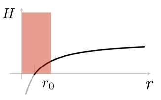
Figure 1: The function $H$ for O$p$-planes with $p<7$ becomes negative at some value $r=r_{0}$ of the radial coordinate. For $3<p<7$, curvature and string coupling become strong already for larger values of $r$, in a region schematically shown in red here.

Instead, one of our main results in this paper is to construct a new class of ten-dimensional de Sitter compactifications of massive IIA. In these new solutions, described in section 3, the O8_- is replaced by an O6_-. As we review in section 2, for such an object, as for any O$p_{-}$-plane with $p<8$, it is well-known that the supergravity solution breaks down in a “hole” region around the source; see Figure 1. In absence of Romans mass, it is known how to resolve this singular behavior in M-theory, where it is replaced by the smooth Atiyah–Hitchin metric [24, 25]; with $F_{0}\neq 0$ however this is not possible.

By modifying an analytic class of AdS solutions [26], we will be able to find numerical de Sitter solutions where the metric takes the form

$$ds^{2}_{10}=e^{2W}ds^{2}_{4}+e^{-2W}(e^{2\lambda_{3}}ds^{2}_{\kappa_{3}}+dz^{2}+e^{2\lambda_{2}}ds^{2}_{S^{2}})~{},$$ (1.1)

where the warp factor $W$ as well as the dilaton and functions $\lambda_{i}$ depend only on the single coordinate $z$, and $ds^{2}_{\kappa_{3}}$ is the metric on an Einstein three-manifold with negative curvature. The $z$ direction parameterizes an interval subject to an orientifold involution. At one side there is an O8₊-plane, on the other side the solution terminates at the boundary of a hole, behaving locally like the O6_- in flat space. There are several AdS solutions where the presence of an O6_- has been argued using this hole behavior, including some with known holographic dual [27, 28].

In section 4, we take a step back from these explicit discussions and analyze in more detail the original solutions of [23] with only O8s. Our discussion here is motivated in part by a complaint [29] about the O-plane singularities in [23]. By using a certain combination of the supergravity equations of motion, [29] claimed that no dS solutions with only O8-plane singularities could exist; they resolved the apparent contradiction with [23] by finding fault with the subleading behavior of the fields as a function of distance from the O8_-.

The argument in [29] assumes the validity of the supergravity equations of motion everywhere, even near the orientifolds where they obviously are invalid. Their apparent aim is to ascertain whether the solution can be trusted in supergravity, before one goes on to consider stringy corrections. Of course as discussed above all de Sitter solutions necessarily involve some correction to the low-energy supergravity approximation. However, such a breakdown does not settle the essential physical question of whether string theory admits de Sitter vacua.

The nature of the solutions of [23], as with all solutions involving orientifolds, is that the supergravity is a valid approximation in one region, while completely breaking down in another. Of course this means that the solutions cannot be completely verified without taking into account the strong-coupling region. However, this issue cannot possibly adjudicated one way or another by using the equations of motion of supergravity.

Nevertheless, in section 4 we discuss the formal problem of the behavior of the supergravity fields and equations in the strong-coupling region of an O8. As one might anticipate, the confusion is one of boundary conditions: [23] and [29] use two slightly different versions, imposing that a certain function have a single or double zero. This comes in turn from two different assumptions on the allowed field fluctuations near O-planes. These issues are in fact independent of the sign of the cosmological constant. There are purely local questions about the correct local description of O8_- singularities. In particular in appendix A we show that certain previously constructed analytic supersymmetric AdS solutions [30] have O8_- singularities with the same boundary behavior as [23].

A priori, without input from a more fundamental theory one cannot determine which, if any of these boundary behaviors is correct. Thus, the status of these O8s is somewhat similar to black brane solutions of supergravity where one requires input from string theory to decide which solutions and singularities are physical. The O6 solutions of section 3 have a similar status. Our analysis of these ensures that they have the correct charge and leading approximation to an orientifold near the boundary of the hole region but leaves the question of whether additional boundary conditions should be imposed presently unanswered.

2 Orientifolds in Supergravity

Since we will have several O$p$-singularities in what follows, we start with a review of their effect in supergravity. We only need in fact O$8$s and O$6$s in this paper, but consider other values below for completeness.

The most common type of O$p$-plane is the so-called O$p_{-}$, which has negative tension and charge. We will mostly focus on this case, commenting only occasionally on O$p_{+}$-planes, which have positive tension and charge, and hence a behavior more similar to a stack of D$p$-branes. In the context of dS solutions discussed in this paper, we will always need at least one O$p_{-}$ to violate the no-go arguments of [3]. We will work in string frame unless otherwise noted.

For general $p$, the O$p_{-}$ solution can be obtained by a modification of the D$p$ solution and reads:

$$ds^{2}=H^{-1/2}ds^{2}_{p+1}+H^{1/2}(dr^{2}+r^{2}ds^{2}_{S^{8-p}})\,,\qquad F_{8-p}=-\frac{4\pi^{7-p}}{v_{8-p}}\text{vol}_{S^{8-p}}\,,\qquad e^{\phi}=g_{s}H^{\frac{3-p}{4}}\,.$$ (2.1)

Here $ds^{2}_{p+1}$ is the space parallel to the O$p$-plane, $v_{d}=2\frac{\pi^{d/2}}{\Gamma(d/2)}$ is the volume of the unit-radius $S^{8-p}$, and $H$ is a harmonic function of the transverse coordinates.

$p=8$.

In this case there is a single transverse coordinate, which we call $x^{9}$; the metric in (2.1) now reads $ds^{2}=H^{-1/2}ds^{2}_{8}+H^{1/2}(dx^{9})^{2}$, with

$$H_{\mathrm{O8}_{-}}=a+\frac{g_{s}}{2\pi}x^{9}\,.$$ (2.2)

For $a>0$ the curvature and string coupling are finite, but at the origin $x^{9}=0$ the string coupling $e^{\phi}=g_{s}a^{-5/4}$ and $R\propto g_{s}^{2}a^{-5/2}$, which may be large if $a$ is small. In particular for $a=0$ they diverge: $e^{\phi}\sim(x^{9})^{-5/4}$, $R\sim(x^{9})^{-5/2}$. At large $x^{9}$ the metric does not reduce to flat space.

An O8₊ is obtained by reversing the sign of the second term in (2.2), so $H_{\mathrm{O8}_{+}}=a-\frac{g_{s}}{2\pi}x^{9}$. Because of the square roots of $H$ in (2.1), the metric now loses meaning beyond a critical distance, $x^{9}\geq 2\pi a/g_{s}$, just like for a stack of D8-branes. This will not be important for our setting, in which the transverse directions are compact. For an O8₊ it is impossible to take $a=0$: it would take the critical distance to zero and make the solution disappear altogether.

$p=7$.

We briefly include this case for completeness, but we will not consider it in this paper. Here

$$H_{\mathrm{O7}_{-}}=\frac{2g_{s}}{\pi}\log\left(\frac{r}{r_{0}}\right)\,.$$ (2.3)

As was the case for the O$8_{-}$, at $r\to\infty$ the metric does not reduce to the flat space metric. For $r<r_{0}$, $H$ becomes negative, and once again the metric becomes imaginary. This unphysical “hole” is resolved in F-theory, where the hole is revealed to contain two mutually non-local $(p,q)$-sevenbranes [36]. The hole also occurs for $p<7$, where a similar resolution is not always known, and we will discuss it at greater length.

For an O7₊, the sign in (2.3) is reversed, and the metric again has a critical distance, as for the O8₊.

$3<p<7$.

The harmonic function is now a power law:

$$H\equiv 1-\left(\frac{r_{0}}{r}\right)^{7-p}\,,\qquad(p<7)\,.$$ (2.4)

The metric becomes imaginary in the “hole”

$$r<r_{0}\propto g_{s}\,;$$ (2.5)

This hole region is a finite distance in the metric and both the curvature and string coupling diverge as one goes towards the “boundary of the hole” $r=r_{0}$: namely

$$R\sim(r-r_{0})^{-5/2}\,,\qquad e^{\phi}\sim(r-r_{0})^{\frac{1}{4}(3-p)}\,.$$ (2.6)

So the solution cannot be trusted already some distance outside the hole. We will return on this issue in section 3.

For O$p_{+}$ in the range $3<p<7$, the sign of the second term in (2.4) is reversed. Now nothing special happens at $r=r_{0}$; as $r\to 0$ the curvature diverges like $R\sim r^{\frac{1}{2}(3-p)}$, while the string coupling goes to zero like $e^{\phi}\sim r^{\frac{1}{4}\frac{p-3}{7-p}}$.

$p=3$.

The harmonic function for an O3_- is still (2.4), but now the string coupling is a constant. The curvature $R$ in fact also vanishes, but the invariant $R_{MN}R^{MN}$ diverges as $\sim(r-r_{0})^{-5}$ as $r\to r_{0}$. So $r=r_{0}$ is still a true singularity.

For the O3₊, the sign in (2.4) is reversed; again $e^{\phi}$ is a constant and $R=0$. Other curvature invariants also remain finite in this case, and it was in fact argued in [37] that the locus at $r\to 0$ is not a singularity, and that one can analytically continue beyond it.

$p<3$.

This case plays no role in four-dimensional compactifications, but let’s review it just the same. At $r=r_{0}$ the curvature again diverges as $(r-r_{0})^{-5/2}$, while the string coupling goes to zero as $e^{\phi}\sim(r-r_{0})^{\frac{1}{4}(3-p)}$. For O$p_{+}$’s in this range, the curvature goes to zero for $r=0$ as $R\sim r^{\frac{1}{2}(3-p)}$, while the string coupling diverges as $e^{\phi}\sim r^{\frac{1}{4}\frac{p-3}{7-p}}$.

3 O8₊–O6_- solutions

In this section we construct a new type of ten-dimensional de Sitter solutions of supergravity, involving O8₊ and O6_- orientifolds. We first present a short review of the ansatz of [23] and then subsequently generalize. In section 3.3 we also show that our ansatz encompasses some analytically known AdS₄ solutions.

3.1 Review of the O8₊–O8_- Ansatz

The simplest class of solutions in [23] are ten-dimensional geometries with a dS₄ factor in spacetime, and two O8-planes. The internal geometry is $S^{1}\times M_{5}$ and only $F_{0}$ flux. The $S^{1}$ is quotiented by an orientifold, so that one can consider an interval $I$ instead.

The metric ansatz was

$$ds^{2}_{10}=e^{2W}ds^{2}_{\mathrm{dS}_{4}}+e^{-2W}\left(dz^{2}+e^{2\lambda}ds^{2}_{M_{5}}\right)\,.$$ (3.1)

$M_{5}$ is a compact Einstein manifold with negative curvature; $z$ is a coordinate on the above-mentioned $S^{1}/\mathbb{Z}_{2}\equiv[0,z_{0}]$. The metric coefficients $W$, $\lambda$, as well as the dilaton $\phi$ are all functions of the coordinate $z$ only.

At the loci $z=0$ and $z=z_{0}$, the metric is singular. The $z=0$ singularity is very mild: the metric is continuous but non-differentiable there. We interpreted this as the backreaction of an O8₊-plane, which has positive tension; in fact we started our analysis by imposing boundary conditions at $z=0$ that correspond to the backreaction of an O8₊. These boundary conditions are not controversial in any way. We then started a numerical evolution, and at $z=z_{0}$ found another singularity. Closer inspection revealed that this matched the behavior of an O8_- at leading order in $|z-z_{0}|$. This led to the claim that we had found a solution with an O8₊ and an O8_-.

Below we describe a new type of solutions, where the O8_- is replaced by an O6_-. We return to a critical analysis of the O8_- solutions and their orientifold boundary conditions in section 4. In particular there we also discuss the arguments of [29].

3.2 Setup

Let us first describe the allowed singularities. We will recognize the O6_- by the behavior at the boundary of its “hole” $r=r_{0}$, discussed in section 2. Adapting that discussion to the $p=6$ case, the local solution reads

$$ds^{2}\sim t^{-1/2}ds^{2}_{\parallel}+t^{1/2}(dt^{2}+ds^{2}_{S^{8-p}})~{},\qquad e^{\phi}\sim t^{-3/4}~{},$$ (3.2)

with $t\equiv r-r_{0}$. Our aim in the following will be to find $\text{dS}_{4}$ solutions where singularities of the type (3.2) are allowed. We will interpret these singularities as boundaries of the holes produced by O6-planes. As we will see, solutions involving singularities (3.2) will in general have free parameters, and a priori we may wonder if more restrictive boundary conditions can or should be imposed to fix them. This is similar to analogous issues that arise for the O8_- solutions which are differed to section 4.

We now look for dS₄ backgrounds of massive type IIA supergravity. We restrict ourselves to a co-homogeneity-one ansatz. For simplicity, we also include an explicit $S^{2}$ factor in the metric, which will be the sphere transverse to the O6-plane. Thus our ansatz for the metric reads

$$ds^{2}_{10}=e^{2W}ds^{2}_{4}+e^{-2W}(e^{2\lambda_{3}}ds^{2}_{\kappa_{3}}+e^{2Q}dz^{2}+e^{2\lambda_{2}}ds^{2}_{S^{2}})~{},$$ (3.3)

with all the functions only depending on the coordinate $z$. The metric $ds^{2}_{\kappa_{3}}$ is an Einstein space with Einstein constant $\kappa_{3}$ and the function $Q$ parametrizes a gauge redundancy.

The most general fluxes compatible with the symmetries of the metric are

$$H=hdz\wedge\text{vol}_{2}~{},\hskip 21.68121ptF_{2}=f_{2}\text{vol}_{2}~{},\hskip 21.68121ptF_{4}=f_{41}\text{vol}_{3}\wedge dz+f_{42}\text{vol}_{4}~{},\hskip 21.68121ptF_{0}\neq 0~{},$$ (3.4)

where a priori $h,f_{2},f_{41}$ and $f_{42}$ are all functions of the coordinate $z$.

3.2.1 Equations of Motion

Away from sources, we can solve the Bianchi identities and equations of motion for the fluxes by setting

$$h=f_{2}^{\prime}/F_{0},\quad f_{42}=\text{cost},\quad f_{41}=\frac{1}{F_{0}}e^{Q-6W-2\lambda_{2}+3\lambda_{3}}(F_{0}c_{1}-f_{42}f_{2}),$$ (3.5)

where $c_{1}$ is an integration constant. The equations for the fluxes are then completely satisfied up to the differential equation

$$f_{2}^{\prime\prime}=e^{2(Q-5W+\phi)}(F_{0}c_{1}f_{42}+(e^{8W}F_{0}^{2}-f_{42}^{2})f_{2})+f_{2}^{\prime}(Q^{\prime}-4W^{\prime}+2\lambda_{2}^{\prime}-3\lambda_{3}^{\prime}+2\phi^{\prime}).$$ (3.6)

This local form of the equation of motion has to be supplemented with boundary conditions for the fluxes, which we are going to discuss in the next section where we focus on a specific choice for the sources.

Turning our attention to the Einstein and dilaton equations of motion, we obtain

$$8\Lambda e^{2q_{0}-4W} = e^{4W-4\lambda_{2}}\left(-\frac{\left(f_{2}^{\prime}\right)^{2}}{F_{0}^{2}}+f_{2}^{2}e^{2q_{0}-2W+2\phi}+F_{0}^{2}e^{2q_{0}-6W+4\lambda_{2}+2\phi}\right)+$$

$$-16\lambda_{2}^{\prime}\phi^{\prime}-24\lambda_{3}^{\prime}\phi^{\prime}+4\left(\lambda_{2}^{\prime}\right){}^{2}+12\left(\lambda_{3}^{\prime}\right)^{2}+24\lambda_{2}^{\prime}\lambda_{3}^{\prime}+$$

$$-6\kappa_{3}e^{2q_{0}-2\lambda_{3}}-4e^{2q_{0}-2\lambda_{2}}+8W^{\prime}\phi^{\prime}-16\left(W^{\prime}\right)^{2}+8\left(\phi^{\prime}\right)^{2}$$ (3.7a)

$$16W^{\prime\prime} = e^{4W-4\lambda_{2}}\left(-\frac{2\left(f_{2}^{\prime}\right)^{2}}{F_{0}^{2}}+6f_{2}^{2}e^{2q_{0}-2W+2\phi}+6F_{0}^{2}e^{2q_{0}-6W+4\lambda_{2}+2\phi}\right)+$$

$$-32\lambda_{2}^{\prime}\phi^{\prime}-48\lambda_{3}^{\prime}\phi^{\prime}+8\left(\lambda_{2}^{\prime}\right){}^{2}+24\left(\lambda_{3}^{\prime}\right){}^{2}+48\lambda_{2}^{\prime}\lambda_{3}^{\prime}+16\left(\phi^{\prime}\right)^{2}+$$

$$-12\kappa_{3}e^{2q_{0}-2\lambda_{3}}-8e^{2q_{0}-2\lambda_{2}}+\frac{\delta_{6}\kappa^{2}\tau_{6}e^{-2\lambda_{2}+q_{0}+W+\phi}}{\pi}+$$

$$+4\delta_{8}\kappa^{2}\tau_{8}e^{q_{0}-W+\phi}-32\lambda_{2}^{\prime}W^{\prime}-48\lambda_{3}^{\prime}W^{\prime}+48W^{\prime}\phi^{\prime}-32\left(W^{\prime}\right)^{2}$$ (3.7b)

$$8\lambda_{2}^{\prime\prime} = e^{4W-4\lambda_{2}}\left(-5\frac{\left(f_{2}^{\prime}\right)^{2}}{F_{0}^{2}}+f_{2}^{2}e^{2q_{0}-2W+2\phi}+5F_{0}^{2}e^{2q_{0}-6W+4\lambda_{2}+2\phi}\right)+$$

$$-24\lambda_{3}^{\prime}\phi^{\prime}-12\left(\lambda_{2}^{\prime}\right){}^{2}+12\left(\lambda_{3}^{\prime}\right)^{2}-6\kappa_{3}e^{2q_{0}-2\lambda_{3}}+4e^{2q_{0}-2\lambda_{2}}+$$

$$+4\delta_{8}\kappa^{2}\tau_{8}e^{q_{0}-W+\phi}+8W^{\prime}\phi^{\prime}-16\left(W^{\prime}\right)^{2}+8\left(\phi^{\prime}\right)^{2}$$ (3.7c)

$$8\lambda_{3}^{\prime\prime} = e^{4W-4\lambda_{2}}\left(-\frac{\left(f_{2}^{\prime}\right)^{2}}{F_{0}^{2}}+5f_{2}^{2}e^{2q_{0}-2W+2\phi}+5F_{0}^{2}e^{2q_{0}-6W+4\lambda_{2}+2\phi}\right)+$$

$$-16\lambda_{2}^{\prime}\phi^{\prime}-8\lambda_{3}^{\prime}\phi^{\prime}+4\left(\lambda_{2}^{\prime}\right){}^{2}-12\left(\lambda_{3}^{\prime}\right){}^{2}+8\lambda_{2}^{\prime}\lambda_{3}^{\prime}+$$

$$+2\kappa_{3}e^{2q_{0}-2\lambda_{3}}-4e^{2q_{0}-2\lambda_{2}}+\frac{\delta_{6}\kappa^{2}\tau_{6}e^{-2\lambda_{2}+q_{0}+W+\phi}}{\pi}+$$

$$+4\delta_{8}\kappa^{2}\tau_{8}e^{q_{0}-W+\phi}+8W^{\prime}\phi^{\prime}-16\left(W^{\prime}\right)^{2}+8\left(\phi^{\prime}\right)^{2}$$ (3.7d)

$$4\phi^{\prime\prime} = e^{4W-4\lambda_{2}}\left(-2\frac{\left(f_{2}^{\prime}\right)^{2}}{F_{0}^{2}}+3f_{2}^{2}e^{2q_{0}-2W+2\phi}+5F_{0}^{2}e^{2q_{0}-6W+4\lambda_{2}+2\phi}\right)+$$

$$-8\lambda_{2}^{\prime}\phi^{\prime}-12\lambda_{3}^{\prime}\phi^{\prime}+\frac{3\delta_{6}\kappa^{2}\tau_{6}e^{-2\lambda_{2}+q_{0}+W+\phi}}{4\pi}+5\delta_{8}\kappa^{2}\tau_{8}e^{q_{0}-W+\phi}+8\left(\phi^{\prime}\right)^{2}$$ (3.7e)

The first equation is a first order equation which will act as a constraint. Each of the other four equations involves a second derivative of a different function, and includes a $\delta$-function that accounts for the back-reaction of the physical sources. Since our 8-dimensional sources are O8₊-planes, which do not suffer from strong-coupling ambiguities, the $\delta_{8}$ terms are well-defined. However, the $\delta_{6}$ terms that appear in the equations of motion are just formal devices since, as we have seen in the flat-space case, for O$p$-planes with $p<7$ their support would be located inside the hole, and hence outside of the physical space-time described by supergravity.

3.2.2 Flux Quantization

From now on, we will focus on solutions with an O8₊ and an O6_-. The orientifold involution is generated by the operators

$$\Omega_{\mathrm{WS}}\sigma_{8}\,,\qquad\Omega_{\mathrm{WS}}(-1)^{\mathrm{F_{\mathrm{L}}}}\sigma_{6}\,.$$ (3.8)

$\Omega_{\mathrm{WS}}$ is the worldsheet parity; $F_{\mathrm{L}}$ is the left-moving fermion number operator; $\sigma_{8}:\,z\mapsto-z$, whose fixed locus is at $z=0$, the O8-plane; and $\sigma_{6}:\,(\theta,\phi)\mapsto(\pi-\theta,-\phi)$ is the antipodal map on the $S^{2}$, whose fixed locus is at the locus where the $S^{2}$ shrinks, the O6-planes. The difference between O$p_{\pm}$ is in general defined via the orientifold action on the Chan–Paton variables, but in cases without D-branes such as this one it can also be defined as a sign appearing for non-orientable maps at the O$p_{+}$, as explained for example in [39, Sec. 6.2]. Early models with O-planes of different signs appearing simultaneously appeared for example in [40, 41, 39].

The $\sigma_{z}$ involution means that the physics in $z<0$ is just a replica of the physics in $z>0$; so, as is often done, we will consider only the latter half. Then, $z$ starts from an O8₊ plane sitting at $z=0$ and ends at the hole of an O6-plane at $z=z_{0}$.

We will restrict our attention to the case

$$F_{4}=0\,.$$ (3.9)

The presence of an O8₊ will make the flux $F_{0}$ jump according to its Bianchi identity:

$$\Delta F_{0}=-\kappa^{2}\tau_{8}\,.$$ (3.10)

Since $F_{0}$ is odd across an O8-plane, we have $\Delta F_{0}=2F_{0}|_{z\rightarrow 0^{+}}$. Combining the two equations we get in our conventions

$$F_{0}|_{z\rightarrow 0^{+}}=\frac{n_{0}^{+}}{2\pi}\,,\qquad n_{0}^{+}=-4\,.$$ (3.11)

The behavior of $F_{2}$ on the O8 plane requires some care. Away from O6/D6 and NS5/ONS5 we have to satisfy the Bianchi identities

$$dF_{2}=F_{0}H\,,\qquad dH=0\,.$$ (3.12)

In particular $H$ does not have to jump. Since on top of an O8₊ plane $F_{0}$ jumps according to (3.10), then $dF_{2}$ has to jump.

The O6 at $z=z_{0}$ is not defined through a $\delta$-function, since the $\delta_{6}$ is outside of the space-time, but through the boundary condition

$$f_{2}(z_{0})=1.$$ (3.13)

This choice fixes the flux quantization for $F_{2}$.

Finally, we have to impose flux quantization for $H$:

$$\int_{M_{3}}H=(2\pi)^{2}N.$$ (3.14)

To do so, we integrate the Bianchi equation on half of the internal space,

$$\int_{\frac{M_{3}}{2}}dF_{2}=\int_{\frac{M_{3}}{2}}F_{0}H,$$ (3.15)

and we use (3.14) and the fact that $H$ as a form is even across the O8₊ to obtain

$$4\pi(f_{2}(z_{0})-f_{2}(0))=F_{0}^{+}\frac{1}{2}(2\pi)^{2}N.$$ (3.16)

By writing $F_{0}\equiv\frac{n_{0}}{2\pi}$ and using (3.13), we get

$$f_{2}(0)=1-\frac{n_{0}^{+}N}{4}$$ (3.17)

where for a simple O8+ (i.e. without D8s on top of it) $n_{0}^{+}=-4$.

Summing up, for a solution of the type O8₊-O6 we have to impose the conditions (3.11), (3.13) and (3.17), which account for the flux quantization of $F_{0}$, $F_{2}$ and $H$.

3.2.3 O8₊ Boundary Conditions and the Cosmological Constant

By integrating the equations of motion across the O8₊plane at $z=0$, we obtain the boundary conditions

$$\lambda_{2}^{\prime}=\lambda_{3}^{\prime}=-\frac{1}{2}F_{0}e^{q_{0}-W+\phi},\qquad W^{\prime}=-\frac{1}{4}F_{0}e^{q_{0}-W+\phi},\qquad\phi^{\prime}=-\frac{5}{4}F_{0}e^{q_{0}-W+\phi},\quad\quad\text{at }z=0.$$ (3.18)

By plugging these conditions into the constraint equation we get

$$\Lambda = \frac{1}{8}f_{2}^{2}e^{-4\lambda_{2}+6W+2\phi}-\frac{3}{4}\kappa_{3}e^{4W-2\lambda_{3}}-\frac{1}{2}e^{4W-2\lambda_{2}}-\frac{(f_{2}^{\prime})^{2}e^{-4\lambda_{2}-2q_{0}+8W}}{8F_{0}^{2}}+$$

$$+ \frac{c_{1}f_{2}f_{42}e^{-4\lambda_{2}-2W+2\phi}}{4F_{0}}-\frac{1}{8}c_{1}^{2}e^{-4\lambda_{2}-2W+2\phi}-\frac{f_{2}^{2}f_{42}^{2}e^{-4\lambda_{2}-2W+2\phi}}{8F_{0}^{2}}-\frac{1}{8}f_{42}^{2}e^{2\phi-6W}$$

$$\text{at }z=0$$

where the second line vanishes for $F_{4}$ = 0. In particular we notice that with $\kappa_{3}$ negative enough we can obtain a positive cosmological constant.

3.3 An Analytic AdS Starting Point

A notable class of already known solutions that fits in our Ansatz (3.3), (3.4), (3.9) can be obtained from the AdS₇ solutions in [27, 42, 43] by replacing simply

$$\mathrm{AdS}_{7}\to\mathrm{AdS}_{4}\times H_{3}\,,$$ (3.20)

where $H_{3}$ is a compact hyperbolic space with the same Einstein constant as AdS₄, $\kappa_{3}=\Lambda$, and doing nothing else. At the level of the equations of motion this replacement has no impact. (At the level of supersymmetry equations it does make a difference; there is a procedure to generate supersymmetric $\mathrm{AdS}_{4}\times H_{3}$ solutions from AdS₇ supersymmetric ones, but it is more complicated and involves also changing the internal metric and fluxes in a certain way [44], in the spirit of [3].)

For the solutions obtained this way, the local form of the metric functions is given by

$$e^{2W}=e^{\lambda_{3}}=\sqrt{2}\pi\sqrt{-\frac{\alpha}{\ddot{\alpha}}}\,,\qquad e^{2\lambda_{2}}=\frac{2\pi^{2}X^{5/2}\alpha^{2}}{X^{5}\dot{\alpha}^{2}-2\alpha\ddot{\alpha}}\,,\qquad q_{0}=2\pi^{2}X^{-5/2}\,,\qquad\Lambda=-\frac{2+X^{5}}{4X^{5/2}}\,;$$ (3.21)

so in particular the metric is given by

$$\frac{1}{\sqrt{2}\pi}ds^{2}_{10}=\sqrt{-\frac{\alpha}{\ddot{\alpha}}}(ds^{{}_{2}}_{\text{AdS}_{4}}+ds^{2}_{H_{3}})+\sqrt{-\frac{\ddot{\alpha}}{\alpha}}X^{-5/2}\left(dz^{2}+\frac{\alpha^{2}}{\dot{\alpha}^{2}-2X^{-5}\alpha\ddot{\alpha}}\right)\,.$$ (3.22)

Reality and positivity of the metric are achieved if

$$\alpha\geq 0\,,\qquad-\ddot{\alpha}>0\,.$$ (3.23)

$F_{2}$ and the dilaton are obtained from

$$e^{\phi}=X^{5/4}\frac{2^{5/4}3^{4}\pi^{5/2}\left(-\frac{\alpha}{\ddot{\alpha}}\right)^{3/4}}{\sqrt{X^{5}\dot{\alpha}^{2}-2\alpha\ddot{\alpha}}},\qquad f_{2}=\frac{\ddot{\alpha}}{23^{4}\pi^{2}}+\frac{F_{0}\pi X^{5}\alpha\dot{\alpha}}{X^{5}\dot{\alpha}^{2}-2a\ddot{\alpha}}\,.$$ (3.24)

(Since we are interested in the case where $F_{0}\neq 0$, we can take $B=\frac{F_{2}}{F_{0}}$, which automatically solves (3.12).) Both values of the constant

$$X=1\,,\qquad X=2^{1/5}$$ (3.25)

lead to a solution of the equations of motion. In AdS₇, the supersymmetric solution is obtained for $X$=1, while the non-supersymmetric one is obtained for $X=2^{1/5}$ [26]. After our replacement (3.20), both cases are non-supersymmetric. However, in what follows we will focus on the $X=2^{1/5}$ case.

The equations of motion force $\alpha$ to be a piece-wise degree 3 polynomial that has to satisfy

$$\dddot{\alpha}=-162\pi^{3}F_{0}\,.$$ (3.26)

If 8-dimensional sources are present, $F_{0}$ changes accordingly to its Bianchi identity, and $\dddot{\alpha}$ jumps. Nevertheless one can impose that the metric and fields are continuous.

Different sources are then chosen by specifying the correct boundary conditions for $\alpha$, which has three free parameters. We highlight the following:

• A D6 is obtained by imposing $\alpha\to 0$.

• The boundary of an O6 hole is obtained with $\ddot{\alpha}\to 0$.

• An O8 requires $\dot{\alpha}\to 0$.

To obtain an O8₊-O6 solution we impose the conditions

$$\dot{\alpha}(0)=0,\qquad\ddot{\alpha}(z_{0})=0,\qquad f_{2}(z_{0})=1,\qquad f_{2}(0)=\frac{k}{2}=1-\frac{n_{0}^{+}N}{4}\quad\,,$$ (3.27)

where both $k$ and $N$ should be integers. The first two conditions in (3.27) come from imposing that at $0$ and $z_{0}$ the solution has the correct local behavior for an O8₊ and for the boundary of an O6_- boundary respectively, as in the list of possibilities above. The third condition fixes the charge of the O6_- (which is $-2$ that of a D6). Finally, the fourth takes care simultaneously of flux quantization for $F_{2}$ at $z=0$, and of flux quantization for $H$, whose flux integral (over the whole space, from $-z_{0}$ to $z_{0}$) is $N$. The two are related by integrating the Bianchi. If we have a simple O8₊ at $z=0$, then $n_{0}^{+}=-4$, and we are only left with the freedom of choosing the integer $N$. Moreover, in this gauge $z_{0}$ depends on $N$ as

$$z_{0}=-\frac{N}{2}+\frac{2}{n_{0}^{+}}=-\frac{N+1}{2},$$ (3.28)

and the requirement that $z_{0}>0$ forces $N<-1$. Explicitly, the solution reads

$$\alpha=\frac{27}{32}\pi^{2}\left(k^{2}(k+12N)+48kz^{2}+64z^{3}\right)\,;$$ (3.29)

recall $k=2(N+1)$.

This solution can be checked using holography: the $a_{\mathrm{Weyl}}$ anomaly can be computed using both field theory and holography as in [45, 43], getting the same result $\frac{16}{7}{2}{15}N^{3}k^{2}$ in the limit where $N\gg 1$ [28].

Curiously, for all AdS₇ solutions with an O6 there is the possibility of analytically continuing past the boundary of the O6 hole. This requires going past the point where $\ddot{\alpha}=0$, to a region where $\ddot{\alpha}>0$, violating (3.23) and making (3.22) imaginary, exactly as for the hole in (2.1), (2.4). The center of this hole is obtained at a point where $\alpha\to 0$, where there is a formal singularity $z=z_{\mathrm{O}}$ similar to the one of a D6 but where some functions have opposite signs. For the solutions (3.29) above, this happens at a point $z_{\mathrm{O}}\sim-N/2$. In general, it is not clear that this procedure of continuing classical supergravity solutions beyond the hole (where they are not valid) has any physical meaning. In our numerical dS₄ solutions below we are not able to completely reproduce this continuation.

3.4 Numerical Solutions

In this section, we show that it is possible to find dS₄ solutions of the type O8-O6, if the O6 is identified by the behavior of the metric and the dilaton near its hole, as in the flat space case (3.2). Imposing these conditions, we are able to explicitly build the numerical solutions. We find a three-parameter family of solutions labeled by the boundary data for the unconstrained metric functions at the boundary of the hole.

We start by building the local solution near an O8₊-plane at $z=0$. By imposing the boundary conditions (3.18) we obtain the expressions

$$e^{-4W} = 1+\frac{F_{0}e^{q_{0}}z}{a_{1}^{3/4}}+\frac{1}{2}e^{2q_{0}}z^{2}\left(-\frac{f_{20}^{2}}{a_{1}^{3/2}a_{2}^{2}}-4\Lambda\right)+O(z^{3})~{},$$

$$e^{-\frac{4}{3}\phi} = a_{1}+\frac{5}{3}\sqrt[4]{a_{1}}F_{0}e^{q_{0}}z+\frac{z^{2}\left(\frac{6a_{1}^{3/2}b^{2}}{F_{0}^{2}}+e^{2q_{0}}(10a_{2}^{2}F_{0}^{2}-9f_{20}^{2})\right)}{18\sqrt{a_{1}}a_{2}^{2}}+O(z^{3})~{},$$

$$e^{-2\lambda_{3}} = 1+\frac{F_{0}e^{q_{0}}z}{a_{1}^{3/4}}+\frac{z^{2}\left(2e^{2q_{0}}\left(a_{2}(a_{2}\Lambda+2)-\frac{2f_{20}^{2}}{a_{1}^{3/2}}\right)+\frac{b^{2}}{F_{0}^{2}}\right)}{6a_{2}^{2}}+O(z^{3})~{},$$ (3.30)

$$e^{2\lambda_{2}} = a_{2}-\frac{a_{2}F_{0}e^{q_{0}}z}{a_{1}^{3/4}}+z^{2}\left(e^{2q_{0}}\left(\frac{a_{2}F_{0}^{2}}{a_{1}^{3/2}}+a_{2}\Lambda+1\right)-\frac{b^{2}}{2a_{2}F_{0}^{2}}\right)+O(z^{3})~{},$$

$$f_{2} = f_{20}+bz+\frac{F_{0}e^{q_{0}}z^{2}(f_{20}F_{0}e^{q_{0}}-a_{1}^{3/4}b)}{2a_{1}^{3/2}}+O(z^{3})~{}.$$

Some comments are in order.

• Since we decided to keep $\Lambda$ and $\kappa_{3}$ as continuous parameters, we fixed the redundancy in the parametrization of the metric by setting $e^{-4W}$ and $e^{-2\lambda_{3}}$ equal to 1 on top of the O8₊.

• $q_{0}$ here is just a gauge redundancy and we can use it to rescale the length of the interval.

• $f_{20}$ and $F_{0}$ are discrete parameters depending on $N$ and $n_{0}$ as in (3.11) and (3.17):

  $$f_{20}=1-\frac{n_{0}^{+}N}{4}~{},\qquad F_{0}=\frac{n_{0}^{+}}{2\pi}~{}.$$ (3.31)

  For a simple O8₊ without D8-branes on top of it we have $n_{0}^{+}=-4$.

• $b$ is not a free parameter. From the first order equation we find:

  $$b=\pm F_{0}e^{q_{0}}\sqrt{\frac{f_{20}^{2}}{a_{1}^{3/2}}-2a_{2}(3a_{2}\kappa_{3}+4a_{2}\Lambda+2)}~{}.$$ (3.32)

  The two roots correspond to the 2 possible choices for the sign of $f_{2}^{\prime}(0)$. We find that only the positive root gives the solutions we are interested in. Moreover, notice that in order to have real solutions the expression inside the square root has to be non-negative. This gives a inequality on the initial parameters of a physically acceptable solution.

To summarize, the local solution near the O8₊-plane depends on four continuous parameters $a_{1},a_{2},\kappa_{3}$ and $\Lambda$ and two discrete ones, $N$ and $n_{0}^{+}$. These parameters have to be chosen such that $b$ defined in (3.32) is real. To hit an O6_- we need to find a point where $f_{2}=1$, requiring one fine-tuning.

We now take an AdS${}_{4}\times H_{3}$ solution at large $N$, i.e. weakly-curved and weakly-coupled, and we slowly increase $\Lambda$ making it positive. Correspondingly, we have to tune the parameters ($\kappa_{3},a_{1},a_{2}$) in order to reach a point $z_{0}$ where, defining $t\equiv|z-z_{0}|$, the functions behave as

$$f_{2}(z_{0})=1,\qquad e^{\lambda_{2}}\sim\text{const},\qquad e^{W}\sim t^{-\frac{1}{4}},\qquad e^{\lambda_{3}}\sim t^{-\frac{1}{2}},\qquad e^{\phi}\sim t^{-\frac{3}{4}}\quad.$$ (3.33)

Near such a point, the metric, the dilaton, and the fluxes have the same local expression as in (3.2). As in that case, the supergravity approximation breaks down near the boundary of hole, since the dilaton starts growing and eventually diverges. Figure 2 shows a typical solution with this behavior.

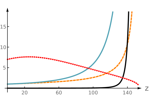
Figure 2: A numerical dS₄ solution with $\Lambda=2.7\times 10^{-3}$ and $\kappa_{3}=-2.1\times 10^{-1}$. It starts from an O8₊-plane (on the left) and ends at the boundary of the hole produced by an O6_--plane (on the right). The functions are $e^{4W}$(turquoise), $e^{4\phi}$(black), $e^{2\lambda_{3}}$(orange, dashed) and $e^{2\lambda_{2}}$(red, dashed). On the right, the functions behave as in equation (3.33).

We have thus succeeded in obtaining dS₄ solutions with an O8₊ at $z=0$ and an O6_- whose boundary lies at $z=z_{0}$. Near this boundary the dilaton and string coupling diverge, but they do in the same way as for the O6 in flat space and for the O6 in the AdS₇ solutions in section 3.3.

As we have mentioned earlier, in this case it is unclear how one should check whether the $\delta$’s in the equations of motion are correctly reproduced, since their support now lies outside the physical space, in the “hole” region where the metric is purely imaginary. Moreover, the integration by parts argument that was in [29] to criticize the O8₊–O8_- solutions of [23] in this case doesn’t apply: if we consider [46, (A.7)], there is no single choice of $c$ that makes both the O8₊ and the O6_- source terms disappear.

Finally, we comment on the physical value of the cosmological constant. At this stage, $\Lambda$ is only a parameter. Its physical value in units of the four dimensional Planck mass is obtained as

$$\Lambda_{\text{phys}}=\frac{\Lambda}{M_{p}^{2}},\qquad\text{with}\quad M_{P}^{2}=\kappa^{2}\text{Vol}_{2}\text{Vol}_{3}\int dze^{Q-4W+2\lambda_{2}+3\lambda_{3}-2\phi}.$$ (3.34)

Performing this integral for the solution in Figure 2 we obtain

$$\Lambda_{\text{phys}}\sim\frac{1}{\kappa^{2}}\text{Vol}_{3}10^{-9}.$$ (3.35)

This small number is expected from the AdS₇ solutions, where at large $N$ the Planck’s mass scales as $N^{5}$ and $\Lambda$ remains constant.

4 A Discussion of the O8₊–O8_- Solutions

In this section we discuss the original O8₊–O8_- de Sitter solutions of [23] in detail. In particular our analysis is focused on the behavior near the O8_-.

In [29], it was claimed that such solutions would be impossible quite generally, based on a certain integration by parts applied to the supergravity equations of motion. They explained the disagreement with [23] by claiming that the $z=z_{0}$ singularity, while displaying the same behavior as an O8_- at leading order in $|z-z_{0}|$, was crucially different from it in subleading behavior. In this section we will investigate this claim.

In appendix A we also exhibit several previously known [30] analytic supersymmetric AdS₄ solutions with O$8_{-}$ planes and the same subleading behavior as our de Sitter solutions.

4.1 The Solutions in Detail

Let us then first look at the equations of motion from the de Sitter solutions of [23] for the functions $W$, $\phi$, $\lambda$ defined in the ansatz (3.1). Since the contentious point is the treatment of O-planes, we include the source terms:

$$W^{\prime\prime}+W^{\prime}(5\lambda-2\phi)^{\prime}-\frac{1}{4}F_{0}^{2}e^{2(\phi-W)}-\Lambda e^{-4W}=\frac{1}{\pi}e^{\phi-W}\sigma\,;$$ (4.1a)

$$(W+2\phi-5\lambda)^{\prime\prime}+W^{\prime}(5\lambda+2\phi)^{\prime}-8(W^{\prime})^{2}-5(\lambda^{\prime})^{2}+\frac{1}{4}F_{0}^{2}e^{2(\phi-W)}=\frac{1}{\pi}e^{\phi-W}\sigma\,;$$ (4.1b)

$$(W-\lambda)^{\prime\prime}+(W-\lambda)^{\prime}(5\lambda-2\phi)^{\prime}+\kappa e^{-2\lambda}+\frac{1}{4}F_{0}^{2}e^{2(\phi-W)}=-\frac{1}{\pi}e^{\phi-W}\sigma\,;$$ (4.1c)

$$4(W^{\prime})^{2}-10(\lambda^{\prime})^{2}-2(\phi^{\prime})^{2}+2\phi^{\prime}(5\lambda-W)^{\prime}+2e^{-4W}\Lambda+\frac{5}{2}\kappa_{5}e^{-2\lambda}-\frac{1}{4}F_{0}^{2}e^{2(\phi-W)}=0\,$$ (4.1d)

where

$$\sigma\equiv\delta(z)-\delta(z-z_{0})\,.$$ (4.2)

is the sum of the O8_± localized contribution.

To focus on the sources, we notice that the second-order equations (4.1a)–(4.1c) are linear combinations of equations of the form

$$e^{W-\phi}\partial_{z}^{2}f_{i}=\pm\frac{1}{\pi}\delta+\ldots\,\qquad(\text{O8}_{\pm})\,.$$ (4.3)

From now on we omit the argument of the $\delta$ when it should be obvious from the context. The $\ldots$ denote terms that are not important near the sources, and

$$f_{i}\equiv\left\{W,\,\frac{1}{5}\phi,\,\frac{1}{2}\lambda\right\}\,.$$ (4.4)

Near the O8₊, the functions are finite; assuming they are also continuous, the treatment of the $\delta$ terms is standard. One can for example take the integral of the sources on a small interval $[-\epsilon,\epsilon]$; in the $\epsilon\to 0$ limit, the only contributions come from the $\delta$ terms and from the discontinuities in the second derivatives. Alternatively, we can directly use the fact that the weak derivative of a discontinuous function $h$ includes a $\delta$ term proportional to the discontinuity; schematically

$$\partial_{z}h=h^{\prime}+(\Delta h)\delta\,.$$ (4.5)

Either way, we obtain

$$e^{W-\phi}f_{i}^{\prime}|_{z\to 0^{+}}=\frac{1}{2\pi}\,\qquad(\text{O8}_{+})\,.$$ (4.6)

The O8_- is more subtle; near its position $z_{0}$, the leading behavior in $z-z_{0}$ of the $f_{i}$ is

$$e^{f_{i}}=c_{i}|z-z_{0}|^{-1/4}+O(|z-z_{0}|^{3/4})\,;$$ (4.7)

so the $f^{\prime}_{i}=\frac{1}{|z-z_{0}|}+{\rm reg}.$, and the $c_{i}$ are such that $e^{W-\phi}=|z-z_{0}|+O(|z-z_{0}|)$.

The logic we just used to obtain (4.6) now does not apply straightforwardly. For example, if we take the integral of (4.3) on $[-\epsilon,\epsilon]$, we have the integral of $e^{W-\phi}\partial_{z}^{2}f_{i}$, which is not a total derivative. If one tries to use (4.5), one is confronted with the derivative of functions $f_{i}$ which are not simply discontinuous but in fact divergent. One could alternatively multiply (4.3) by $e^{\phi-W}$, and then integrate it on $[-\epsilon,\epsilon]$. Now the left-hand side $\partial_{z}^{2}f_{i}$ is a total derivative, but the right-hand side reads

$$e^{\phi-W}\delta\sim\frac{1}{|z-z_{0}|}\delta(z-z_{0})$$ (4.8)

which is a product of distributions, of unclear interpretation.

In fact this formal trouble hides an even deeper problem: since the dilaton and curvature are diverging at the O8_-, the supergravity approximation is breaking down there, and we shouldn’t use the equations of motion (4.1) in the first place. Our numerical solution cannot be trusted there, and trying to understand its formal properties is not physically meaningful. The reason we identified our divergence with that of an O8_- was that its leading-order divergence in $(z-z_{0})$ behaves exactly like an O8_- solution in flat space. That solution also has the problem that supergravity breaks down in its vicinity, but it is believed to be modified in fully-fledged string theory, whatever its equations of motion may be, but to still exist.

More precisely, both the flat-space O8_- and our solution satisfy

$$e^{W-\phi}f_{i}^{\prime}|_{z\to z_{0}^{+}}=-\frac{1}{2\pi}\,\qquad(\text{O8}_{-})\,$$ (4.9)

as one can see from (4.7). This is very similar to (4.9); for an O8_- where the dilaton and curvature remains small ($a\gg 1$, in the language of footnote 10 and (2.2)), this could be motivated by the same arguments that took us to (4.9).

This similarity between our singularity and the flat-space O8_- motivates the hope that our solution also exists in fully-fledged string theory. Notice that the solution has a supergravity “modulus” $c$, generated by the rescaling

$$g_{MN}\to e^{2c}g_{MN}\,,\qquad\phi\to\phi-c\,.$$ (4.10)

This is a symmetry of the supergravity equations of motion, but not of full string theory. We thus expect the solution to exist in string theory only for a particular value of $c$. (We will see later that it is not clear whether $c$ can in fact be considered a field in an effective four-dimensional description.) However, as stated in [23], all this is unproven until one somehow finds a way to evaluate the stringy corrections: there might be no value of $c$ for which the solution works in full string theory.

Meanwhile, [29] examined the same solution by using the supergravity equations of motion even in the region where supergravity breaks down. This should not be done, and that the fate of the solution cannot possibly be decided this way. It is true that we ourselves used supergravity, but we just looked at the leading behavior of the fields in $|z-z_{0}|.$ In particular this allows us to read off the correct charge of the O8_-. However, it is not clear that applying the uncorrected supergravity equations of motion to the subleading behavior as in [29] makes any physical sense. For the rest of this section we will consider this issue further.

4.2 Various Versions of the Boundary Conditions

As we just saw, the solutions in [23] satisfy (4.9). However, (4.9) would seem to suffer from an ambiguity. For example one might want to rewrite it as

$$f_{i}^{\prime}|_{z\to z_{0}^{+}}=-\frac{1}{2\pi}e^{W-\phi}|_{z\to z_{0}^{+}}\,.$$ (4.11)

From (4.7) we now see that both sides have a simple pole; so the equation is of the form

$$\frac{d_{i}^{\mathrm{L}}}{|z-z_{0}|}+e_{i}^{\mathrm{L}}=\frac{d_{i}^{\mathrm{R}}}{|z-z_{0}|}+e_{i}^{\mathrm{R}}\,.$$ (4.12)

Equality of the leading term, $d_{i}^{\mathrm{L}}=d_{i}^{\mathrm{R}}$, is equivalent to (4.9); but if we also impose equality of the subleading coefficient $e_{i}^{\mathrm{L}}=e_{i}^{\mathrm{R}}$ we have a more restrictive boundary condition than (4.9). By multiplying (4.9) by a diverging function, we have made one more coefficient of its Taylor expansion emerge; this new coefficient has effectively created an extra boundary condition. Thus (4.11) is not in fact equivalent to (4.9); we will call them the restrictive and permissive boundary conditions, respectively.

One could be even more perverse and multiply (4.9) by an even more diverging function, such as $e^{2(W-\phi)}$. The two sides of the equation would now be of the form

$$\frac{d_{i}^{\mathrm{L,R}}}{|z-z_{0}|^{2}}+\frac{e_{i}^{\mathrm{L,R}}}{|z-z_{0}|}+f_{i}^{\mathrm{L,R}}\,,$$ (4.13)

thus creating the need to equate even the coefficients $f_{i}^{\mathrm{L,R}}$. While of course this does not appear particularly natural, one does not see any a priori reason to consider this option to be any less valid than (4.9) or (4.11). Clearly we need a better understanding of this ambiguity.

The restrictive boundary condition (4.11) is effectively the one used in [29]; it is not satisfied by the singularity we identified as O8_- in [23], and this is what creates the apparent contradiction between the two papers.

More precisely, [29] applies (4.11) to the difference

$$(f_{1}-f_{2})^{\prime}=W^{\prime}-\frac{1}{5}\phi^{\prime}\,,$$ (4.14)

which from (4.12) we see to be of the form $\frac{\Delta d_{12}}{|z-z_{0}|}+\Delta e_{12}=0$ for some constants $\Delta d_{12}$ and $\Delta e_{12}$. The restrictive (4.11) imposes $(f_{1}-f_{2})^{\prime}=0$, so both $\Delta d_{12}=\Delta e_{12}=0$; the permissive (4.9) imposes $e^{W-\phi}(f_{1}-f_{2})^{\prime}=0$, so only $\Delta d_{12}=0$. Our solution in [23] satisfies $\Delta d_{12}=0$: it cancels the pole in $(f_{1}-f_{2})^{\prime}$, but not the constant.

In other words, [29] can be read as a complaint that in $(f_{1}-f_{2})^{\prime}$ we only made sure that the pole $\frac{\Delta d_{12}}{|z-z_{0}|}$ vanished, and not the constant term $\Delta e_{12}$. Indeed they went further: with an integration by parts, they showed that no solution with only O8-planes exists such that this constant term vanishes. So the issue is really reduced to whether we should use their restrictive boundary conditions (4.11) for $(f_{1}-f_{2})^{\prime}=W^{\prime}-\frac{1}{5}\phi^{\prime}$, or our permissive ones. Let us stress once again, however, that one really should be looking at the full string theory equations of motion.

4.3 Action Variation

We will now see that the difference between permissive and restrictive boundary conditions (4.9), (4.11) can be traced back to how one varies the action: namely, to what space the variations $\delta f_{i}$ are taken to belong. We will illustrate this point by focusing on the dilaton’s equation of motion.

The relevant terms of the action in the string frame are

$$S^{0} =\frac{1}{\kappa^{2}}\int_{M_{10}}d^{10}x\sqrt{-g}\,\left[e^{-2\phi}\left(R+4(\nabla\phi)^{2}\right)-\frac{1}{2}F_{0}^{2}\right]\,,$$ (4.15)

$$S^{\mathrm{DBI}} =-\sum\tau_{i}\int_{\Sigma_{i}}d^{9}xe^{-\phi}\sqrt{-h}\,,$$ (4.16)

where $\Sigma_{i}$ are the sources, and $h_{MN}$ is the metric induced on them by the bulk metric.

Our point of view in this subsection will be that the internal space

$$M_{5}\times[0,z_{0}]\,,$$ (4.17)

whose boundary consists of the loci where the two O8-planes sit. Thus we should be careful to include boundary terms. First of all, the variation of a bulk term in the action can yield a boundary term when we integrate by parts to extract its equations of motion. For example, the dilaton kinetic term in (4.15), when varied with respect to $\phi$, upon integration by parts produces a bulk term that contributes to the equations of motion, but also a boundary term

$$8\int_{\partial M_{10}}d^{9}x\sqrt{-h}\,e^{-2\phi}n^{M}\partial_{M}\phi\,,$$ (4.18)

where $n^{M}$ is the normal vector to $\partial M_{10}$, normalized so that $n^{2}\equiv g^{NM}n_{N}n_{M}=1$. Second, as usual in general relativity, in presence of a boundary the action should also contain the Gibbons–Hawking–York (GHY) boundary term, even prior to variation. Varying the usual Einstein–Hilbert action produces a term containing the normal derivative of the metric variation $n^{M}\partial_{M}\delta g_{NP}$, which would require a restricted variational problem. The GHY term cancels this variation. In the Einstein frame it is equal to the integral of the boundary extrinsic curvature:

$$S^{\mathrm{GHY,E}}=\frac{2}{\kappa^{2}}\int_{\partial M_{10}}d^{9}x\sqrt{-h_{\mathrm{E}}}\,\nabla^{\mathrm{E}}_{M}n^{M}_{\mathrm{E}}\,.$$ (4.19)

In the string frame, a GHY-like term that achieves the same cancellation is

$$S^{\mathrm{GHY}}=\frac{2}{\kappa^{2}}\int_{\partial M_{10}}d^{9}x\sqrt{-h}\,e^{-2\phi}\nabla_{M}n^{M}\,.$$ (4.20)

Notice that (4.20) does not immediately turn into (4.19) upon the usual change of frame $g^{\mathrm{E}}_{MN}\equiv e^{-\phi/2}g_{MN}$. Rather, it does so when one combines it with a further boundary term produced by changing frame. Indeed

$$\int_{M_{10}}d^{10}x\sqrt{-g_{\mathrm{E}}}\,\left(R_{\mathrm{E}}-\frac{1}{2}(\nabla\phi)^{2}-\frac{1}{2}e^{\frac{5}{2}\phi}F_{0}^{2}\right)\equiv S^{0}_{\mathrm{E}}=S^{0}+\frac{9}{2\kappa^{2}}\int_{\partial M_{10}}d^{9}x\sqrt{-h}e^{-2\phi}n^{M}\partial_{M}\phi\,,$$ (4.21)

and

$$S^{\mathrm{GHY,E}} =\frac{2}{\kappa^{2}}\int_{\partial M_{10}}d^{9}x\frac{\sqrt{-h}}{\sqrt{-g}}e^{\frac{1}{4}\phi}\partial_{M}(e^{-\frac{9}{4}\phi}\sqrt{-g}g^{MN}n_{N})=$$

$$=\frac{2}{\kappa^{2}}\int_{\partial M_{10}}d^{9}x\sqrt{-h}\,e^{-2\phi}\left[\frac{1}{\sqrt{-g}}\partial_{M}(\sqrt{-g}g^{MN}n_{N})-\frac{9}{4}\partial_{M}\phi g^{MN}n_{N}\right]$$ (4.22)

$$=\frac{2}{\kappa^{2}}\int_{\partial M_{10}}d^{9}x\sqrt{-h}\,e^{-2\phi}\nabla_{M}n^{M}-\frac{9}{2\kappa^{2}}\int_{\partial M_{10}}d^{9}x\sqrt{-h}\,e^{-2\phi}n^{M}\partial_{M}\phi\,.$$

So $S^{0}+S^{\mathrm{GHY}}=S^{0}_{\mathrm{E}}+S^{\mathrm{GHY,E}}$.

The total string-frame action is then

$$S_{1/2}=S^{0}+\frac{1}{2}S^{\mathrm{DBI}}+S^{\mathrm{GHY}}\,.$$ (4.23)

(The subscript _1/2 reminds us that we are working with half of spacetime; the factor $1/2$ in front of the DBI action is present for the same reason.) Let us vary it with respect to the dilaton. The bulk variation produces (4.1b); but we are now interested in the boundary terms. The boundary contribution of $\delta S_{0}$ is (4.18); $S^{\mathrm{DBI}}$ are already localized on the boundary, and also contribute. In particular notice that $\delta S^{\mathrm{GHY}}$ is non-zero because of the $e^{-2\phi}$ factor, which is absent in the Einstein frame. Evaluating it explicitly in our metric ansatz (3.1) gives

$$\delta_{\phi}S^{\mathrm{GHY}} =-\frac{4}{\kappa^{2}}\int_{\partial M_{10}}d^{9}x\sqrt{-h}\delta\phi e^{-2\phi}\,\nabla^{M}n_{M}=-\frac{4}{\kappa^{2}}\mathrm{Vol}_{\mathrm{dS}_{4}}\mathrm{Vol}_{M_{5}}\delta\phi e^{-2\phi+W}\partial_{z}(e^{-W+5\lambda})$$

$$=-\frac{4}{\kappa^{2}}\mathrm{Vol}_{\mathrm{dS}_{4}}\mathrm{Vol}_{M_{5}}\delta\phi e^{-2\phi+5\lambda}(5\lambda-W)^{\prime}|_{z\to z_{0}^{+}}\,$$ (4.24)

taking into account that $n^{2}=1$. Combining all the contributions we obtain

$$\kappa^{2}\delta_{\phi}S=4\mathrm{Vol}_{\mathrm{dS}_{4}}\mathrm{Vol}_{M_{5}}e^{-W+5\lambda-\phi}\delta\phi\left(e^{W-\phi}(2\phi^{\prime}+W^{\prime}-5\lambda^{\prime})\mp\frac{1}{2\pi}\right)|_{z\to z_{0}^{+}}\,.$$ (4.25)

At the O8₊, (4.25) is a linear combination of the (4.6). At the O8_-, from (4.7) we see that the prefactor $e^{-W+5\lambda-\phi}\sim\frac{1}{|z-z_{0}|}$:

$$\begin{split}0&=\frac{1}{|z-z_{0}|}\delta\phi\left(e^{W-\phi}(2\phi^{\prime}+W^{\prime}-5\lambda^{\prime})+\frac{1}{2\pi}\right)|_{z\to z_{0}^{+}}\\ &=\frac{1}{|z-z_{0}|}\delta\phi\left(d+e|z-z_{0}|+\ldots\right)\end{split}\,\qquad(\text{O8}_{-})\,.$$ (4.26)

These $d$ and $e$ are related to our notation in (4.12). So now the interpretation of (4.26) depends on the boundary condition one imposes on the fluctuation $\delta\phi$; or in other words, to what space $\delta\phi$ belongs. At first sight, a few possibilities might spring to mind:

• $\delta\phi\in L^{2}(M_{10})$. Since $\sqrt{g}$ diverges as $\frac{1}{|z-z_{0}|^{2}}$ on the O8_-, this requires $\delta\phi\to 0$; if it goes like a power law, $\delta\phi\sim|z-z_{0}|^{\alpha}$, then $\alpha>1/2$. Then (4.26) only requires setting the leading order $d=0$. So we are getting a linear combination of the permissive boundary conditions (4.9).

• $\delta\phi$ smooth. In particular its limit for $z\to z_{0}$ can be a non-zero constant; this requires both the leading and subleading order, $d=e=0$. In this case we are getting a linear combination of the restrictive boundary conditions (4.11).

Intuitively, the more permissive we are with our variation space, the more restrictive the boundary conditions, because we are varying in more directions in field space.

The two possibilities we have just seen are just some natural-sounding possibilities; others can be considered. The permissive boundary conditions are obtained more generally for any boundary condition that forces $\delta\phi\to 0$. Making $\delta\phi\sim|z-z_{0}|^{\alpha}$, $\alpha>1$ would impose no boundary conditions at all; at the opposite extreme, leaving $\delta\phi$ completely unconstrained, free to diverge, would impose infinitely many boundary conditions. In section 4.5 we will try to get a more physical picture of what might be reasonable conditions on $\delta\phi$.

We are now going to look at the same issue from a slightly different viewpoint, using delta functions and distributions.

4.4 Delta-Function Sources

We now consider the internal space as

$$M_{5}\times S^{1}\,,$$ (4.27)

where $S^{1}=[0,2z_{0}]$ with the periodic identification $2z_{0}\cong 0$, and the functions are now required to be even under $z\to-z$.

From this point of view, there is no boundary, and no need to include boundary GHY terms; the action is now

$$S=S^{0}+S^{\mathrm{DBI}}$$ (4.28)

with (4.15), (4.16). We can rewrite the localized DBI terms as a bulk term including a delta function, and then vary. This is how we found the equations of motion (4.1), but the discussion so far (and in particular the difference between (4.9) and (4.11)) made it clear that it is crucial to also understand how the variation multiplies it; so let us see this in more detail. We again focus on the dilaton equations of motion:

$$\kappa^{2}\delta_{\phi}S =-4\int_{M_{10}}d^{10}x\sqrt{-g}\delta\phi e^{-2\phi}(-2R-8(\nabla e^{-\phi})^{2})-\sum_{i}\tau_{i}\int_{\Sigma_{i}}d^{9}x\sqrt{-h}\delta\phi e^{-\phi}$$

$$=-4\int dze^{-W+5\lambda-\phi}\delta\phi\left(e^{W-\phi}(W+2\phi-5\lambda)^{\prime\prime}+\ldots+\frac{1}{\pi}\sigma\right)\,.$$ (4.29)

The parenthesis is nothing but the equations of motion (4.1b), and again the $\ldots$ are terms irrelevant for our discussion of what happens near the O8_±. Recalling (4.7), we have obtained that (4.1b) in fact arises as

$$\frac{1}{|z-z_{0}|}\delta\phi\left(e^{W-\phi}(W+2\phi-5\lambda)^{\prime\prime}+\ldots+\frac{1}{\pi}\delta\right)=0\qquad(\text{O8}_{-})\,.$$ (4.30)

This is the delta-function counterpart of (4.26). Once again we see that the conditions we impose on $\delta\phi$ play a crucial role. Mirroring our discussion in the previous subsection:

• $\delta\phi\in L^{2}(M_{10})$. Then $\delta\phi\to 0$; in this case the second derivatives produces a delta term to match the explicit $\delta$ in the parenthesis; the subleading terms in the $|z-z_{0}|$ expansion evaluate to zero when multiplied by the prefactor $\frac{\delta\phi}{|z-z_{0}|}$. Thus in this case we only have a condition on the leading behavior.

• $\delta\phi$ smooth. This in particular allows $\delta\phi$ to go to a constant. Then we have a term $\frac{1}{|z-z_{0}|}\delta(z-z_{0})$, as anticipated in (4.8). This is of unclear interpretation, but if it can be given a meaning, it is likely to require two conditions on $e^{W-\phi}(W+2\phi-5\lambda)^{\prime\prime}$ and thus on the functions: not just a condition on their leading behavior, but on their subleading behavior as well.

So we recover the issue we saw in the previous subsection, although with the disadvantage of having products of distributions. This is expected as General Relativity is a non-linear theory, and only in very particular cases the field equations become linear allowing for a rigorous treatment of the singularities within the framework of usual linear distribution theory. This is the case for the flat-space solutions described in section 2, where the field equations reduce to a Gauss-like equation for the harmonic function $H$ of the form $\Delta H=\tau\delta$. In more general cases, like the present one, the non-linearity of the field equations introduces ill-defined products of distributions.

Given the problems we have just seen with interpreting the $\delta$ terms, we might wonder whether perhaps we are working in the wrong set of variables. Perhaps the issues are created by the fact that the $f_{i}$ are diverging, and it might be wiser to switch to variables that remain finite.

For example we can define

$$H_{i}=e^{-4f_{i}}\,;$$ (4.31)

the metric then reads

$$ds^{2}_{10}=H_{1}^{-1/2}ds^{2}_{dS_{4}}+H_{1}^{1/2}(dz^{2}+H_{3}^{-1}ds^{2}_{M_{5}})\,.$$ (4.32)

The equations of motion are now

$$\Lambda=\frac{F_{0}^{2}\sqrt{\frac{H_{1}}{H_{2}}}}{8H_{1}H_{2}^{2}}-\frac{5H_{3}\kappa}{4H_{1}}-\frac{(H_{1}^{\prime})^{2}}{8H_{1}^{3}}+\frac{25(H_{2}^{\prime})^{2}}{16H_{1}H_{2}^{2}}+\frac{5(H_{3}^{\prime})^{2}}{4H_{1}H_{3}^{2}}+\frac{5H_{1}^{\prime}H_{2}^{\prime}}{16H_{1}^{2}H_{2}}-\frac{25H_{2}^{\prime}H_{3}^{\prime}}{8H_{1}H_{2}H_{3}}$$ (4.33a)

$$\pm\frac{4}{\pi}\sigma=-\frac{H_{2}^{5/4}H_{1}^{\prime\prime}}{H_{1}^{5/4}}-\frac{F_{0}^{2}\sqrt[4]{H_{1}}}{H_{2}^{5/4}}-4H_{1}^{3/4}H_{2}^{5/4}\Lambda+\frac{H_{2}^{5/4}(H_{1}^{\prime})^{2}}{H_{1}^{9/4}}-\frac{5\sqrt[4]{H_{2}}H_{1}^{\prime}H_{2}^{\prime}}{2H_{1}^{5/4}}+\frac{5H_{2}^{5/4}H_{1}^{\prime}H_{3}^{\prime}}{2H_{1}^{5/4}H_{3}}$$ (4.33b)

$$\pm\frac{4}{\pi}\sigma=-\frac{H_{2}^{5/4}H_{3}^{\prime\prime}}{\sqrt[4]{H_{1}}H_{3}}-\frac{F_{0}^{2}\sqrt[4]{H_{1}}}{H_{2}^{5/4}}-\frac{2H_{2}^{5/4}H_{3}\kappa}{\sqrt[4]{H_{1}}}-2H_{1}^{3/4}H_{2}^{5/4}\Lambda+\frac{7H_{2}^{5/4}(H_{3}^{\prime})^{2}}{2\sqrt[4]{H_{1}}H_{3}^{2}}-\frac{5\sqrt[4]{H_{2}}H_{2}^{\prime}H_{3}^{\prime}}{2\sqrt[4]{H_{1}}H_{3}}$$ (4.33c)

$$\pm\frac{4}{\pi}\sigma =-\frac{\sqrt[4]{H_{2}}H_{2}^{\prime\prime}}{\sqrt[4]{H_{1}}}-\frac{4F_{0}^{2}\sqrt[4]{H_{1}}}{5H_{2}^{5/4}}-\frac{2H_{2}^{5/4}H_{3}\kappa}{\sqrt[4]{H_{1}}}-\frac{8}{5}H_{1}^{3/4}H_{2}^{5/4}\Lambda-\frac{H_{2}^{5/4}(H_{1}^{\prime})^{2}}{5H_{1}^{9/4}}+\frac{2H_{2}^{5/4}(H_{3}^{\prime})^{2}}{\sqrt[4]{H_{1}}H_{3}^{2}}$$

$$+\frac{\sqrt[4]{H_{2}}H_{1}^{\prime}H_{2}^{\prime}}{2H_{1}^{5/4}}-\frac{5\sqrt[4]{H_{2}}H_{2}^{\prime}H_{3}^{\prime}}{2\sqrt[4]{H_{1}}H_{3}}+\frac{(H_{2}^{\prime})^{2}}{\sqrt[4]{H_{1}}H_{2}^{3/4}}\,.$$ (4.33d)

Near the O8_-, (4.7) tells us that $H_{i}\sim c_{i}^{-4}|z-z_{0}|$. Looking at (4.33), we see that the coefficients of $H_{i}^{\prime\prime}$ are all constant; taking this into account, near the O8_- now the equations are of the form $\partial_{z}^{2}H_{i}=\delta$ rather than the more confusing (4.3). But notice that this agreement only required the leading behavior in $z-z_{0}$; so from this point of view the permissive boundary conditions seem to be enough to reproduce the delta’s in the equations of motion.

4.5 Finite Masses

We have seen in detail how the problem of the boundary conditions can be traced back to the boundary conditions for the field fluctuations. Let us now look at a possible strategy one might try to use to decide the correct conditions for the field fluctuations.

Namely, one might try to perform a KK reduction on a solution. We work in the point of view where the internal space is $M_{5}\times S^{1}$, as in section 4.4. Unfortunately this is a very convoluted computation, but we can try to look at a small block in the mass matrix; once again we will consider the dilaton fluctuations $\delta\phi$. The second variation of the action reads

$$\delta^{2}_{\phi}S=\frac{8}{\kappa^{2}}\int_{M_{10}}d^{10}x\sqrt{-g}e^{-2\phi}\nabla_{m}\delta\phi\nabla^{m}\delta\phi+\sum_{i}\tau_{i}\int_{\Sigma_{i}}d^{9}x\sqrt{-h}e^{-\phi}\delta\phi^{2}\,.$$ (4.34)

We now expand the dilaton perturbation on not-yet-specified basis of functions in the internal space:

$$\delta\phi=\sum_{k}\varphi_{k}(x)f_{k}(y)\,,$$ (4.35)

where $x$ and $y$ denote external and internal coordinates respectively. Plugging this into (4.34) we get

$$\delta^{2}_{\phi}S=\int_{M_{4}}\sqrt{-g_{4}}d^{4}x\Big{[}g_{4}^{\mu\nu}\partial_{\mu}\varphi_{i}\partial_{\nu}\varphi_{j}\frac{8}{\kappa^{2}}\int_{M_{5}}d^{5}y\int dz\sqrt{g_{5}}e^{-4W+5\lambda-2\phi}f_{i}f_{j}$$ (4.36)

$$+\varphi_{i}\varphi_{j}\int_{M_{5}}d^{5}y\sqrt{g_{5}}\Big{(}e^{-W+5\lambda-\phi}f_{i}f_{j}+\frac{8}{\kappa^{2}}\int dz\Big{(}e^{5\lambda-2\phi}f_{i}^{\prime}f_{j}^{\prime}+e^{3\lambda-2\phi}g_{5}^{ab}\partial_{a}f_{i}\partial_{b}f_{j}\Big{)}\Big{)}\Big{]}\,.$$

Now the $\varphi_{i}$ are interpreted as four-dimensional scalar fields. The first line in (4.36) gives their kinetic terms, while the second line gives their mass matrix. We see that some of the terms might diverge. Let us consider for example the boundary condition where $f$ is taken to be smooth, which as we saw earlier leads to the restrictive boundary conditions. In this case, all the terms containing an integral in $dz$ converge; but the term $e^{-W+5\lambda-\phi}f_{i}f_{j}$, which comes from the localized term in (4.34), goes like $\frac{1}{|z-z_{0}|}f_{i}f_{j}$ and hence diverges for $f_{i}$ smooth. So the restrictive boundary conditions in this case lead to a diverging mass matrix, which is presumably unphysical.

On the other hand, if we take $f_{i}\sim|z-z_{0}|^{\alpha}$ with $\alpha>1/2$, which according to (4.26) leads to the permissive boundary conditions, then this block in the mass matrix is finite.

We hasten to add, however, that this is only a very small piece of the KK reduction. In order to compute the mass matrix, one actually needs to first make sure all the fields with different spins in four dimensions to decouple, and this might change the block of the mass matrix we have computed above. It is possible to imagine that other naively divergent terms appear, and that they combine with the one we have discussed here to give a finite mass. We even saw a possible indication of this in the analogue of (4.36) in the Einstein frame. Even if this happens, however, such a cancellation of infinities seem to depend on the “scheme” one chooses to regularize the infinities, similar to our discussion of the on-shell action in section 4.6.

To summarize: depending on the boundary conditions on the fluctuations, one will obtain a larger or smaller set of fields in four dimensions. The restrictive boundary conditions on the fields correspond to a laxer condition on the fluctuations, which would result in more four-dimensional scalar fields $\varphi_{i}$. The 4d equations of motion for the additional fields obtained in this way would presumably not be obeyed, thus invalidating our solutions from another point of view. However, we found in this subsection that these putative additional $\varphi_{i}$ seem in fact to have an infinite mass matrix.

4.6 On-Shell Action

In the previous subsection we examined our solutions from the point of view of the four-dimensional effective action. We focussed on small fluctuations, interpreting them as scalars in four dimensions. In this section, we will focus instead on the parameter $c$ in (4.10).

If stringy corrections are not considered, $c$ appears to be a modulus of our solutions. As we discussed earlier, (4.10) is only a symmetry of the supergravity equations of motion, and not of those of full string theory; so $c$ will be fixed in the full theory. In other words, there will be an effective potential $V(c)$; the question of existence of our solutions in full string theory is the same as the existence of an extremum of this potential. $V(c)$ will have contributions from all stringy corrections, and for this reason it is difficult to compute. In a way the complaint in [29] amounts to saying that supergravity also gives a contribution to $V(c)$. As we discussed, however, in the strongly-coupled region supergravity is the least important term in the equations of motion, and so its contribution will be completely swamped by more important ones.

However, the spirit of this section has been to examine the formal problem of the existence of the solutions in supergravity. In that spirit, let us try to see how one should interpret $c$. If it can be interpreted as a scalar field in four dimensions, then it would enter the four-dimensional action:

$$S_{4d}=\int\sqrt{-g_{4}}(R_{4}-V(c))\,.$$ (4.37)

However, we quickly see a puzzle. The rescaling (4.10) acts on the four-dimensional metric as $g_{\mu\nu}\to e^{2c}g_{\mu\nu}$. The Ricci scalar $R_{4}\to e^{-2c}R_{4}$. For a shift in $c$ to be a symmetry, we would need the potential to rescale in the same way, $V(c)=V_{0}e^{-2c}$. This does not seem to be compatible with a potential that has a vacuum, unless the constant $V_{0}=0$, i.e. the vacuum is Minkowski.

The resolution of this puzzle is clear given our discussion in section 4.5: $c$ cannot be viewed as a field. Indeed, the infinitesimal counterpart of (4.10) corresponds to fluctuations

$$\delta g_{\mu\nu}=2g_{\mu\nu}\delta c\,,\qquad\delta g_{mn}=2g_{mn}\delta c\,,\qquad\delta\phi=-\delta c\,.$$ (4.38)

Looking at our (4.26) and our discussion there, we see that this would require a boundary condition where the two leading coefficients $d$ and $e$ should be set to zero; this is the restrictive condition (4.11). Similar conclusions can be reached with (4.30). So when $c$ can be considered as a field, our solutions don’t exist; this is consistent with (4.37).

On the other hand, with the boundary conditions (4.9) we have imposed, $\delta c$ is not part of the space of allowed field variations.

What if we try to evaluate (4.37) directly? After all, we should be able to compute its value by integrating on the solution the ten-dimensional $S$ over $M_{6}$, for any value of $c$. (Equivalently, we can integrate $S$ over $M_{10}$; this would diverge because of the volume of de Sitter space, but we can take care of this by analytically continuing to Euclidean signature.)

Perhaps unsurprisingly at this point, the answer is that the Lagrangian density is divergent at the O8_-, and so this on-shell action is ill-defined. The computation is similar to (4.29). The bulk action (4.15) diverges on shell as $\int dz\frac{1}{|z-z_{0}|^{2}}$:

$$\begin{split}\kappa^{2}S^{0}\propto&\int dz\Big{[}2e^{5\lambda-2\phi}\Big{(}(5\lambda-W)^{\prime\prime}\\ &+4(W^{\prime})^{2}-5W^{\prime}\lambda^{\prime}+15(\lambda^{\prime})^{2}-2(\phi^{\prime})^{2}\Big{)}-\frac{1}{2}e^{5\lambda-2W}F_{0}^{2}\Big{]}+\ldots\,.\end{split}$$ (4.39)

The O8_- term is even more puzzling:

$$S^{\mathrm{DBI}}\propto e^{-W+5\lambda-\phi}|_{z=z_{0}}=\int dze^{-W+5\lambda-\phi}\delta(z-z_{0})\,,$$ (4.40)

so it again would involve evaluating $\frac{1}{|z-z_{0}|}\delta(z-z_{0})$, an expression which has plagued our discussion since (4.8).

It is possible to find regularization schemes that make the divergences in (4.39) and (4.40) cancel each other, and leave a finite answer. For example, we can decide to introduce a length cutoff: we can evaluate the integral in (4.39) only up to $z_{0}-\epsilon$, and interpret (4.40) as $e^{-W+5\lambda-\phi}|_{z=z_{0}-\epsilon}$. The divergences in $S^{0}+S^{\mathrm{DBI}}$ now do cancel, and leave a finite result, which one might try to interpret as (4.37). However, this regularization scheme is highly arbitrary. It is equivalent to regularizing $\delta(z-z_{0})$ as $\frac{1}{2}\left(\delta(z-z_{0}+\epsilon)+\delta(z-z_{0}-\epsilon)\right)$. More conventional regularizations for $\delta(z-z_{0})$, where for example one replaces it with a Gaussian of width $\epsilon$, would give different results, or fail to cancel the divergence altogether.

So a direct attempt at computing (4.37) by regularizing $S=S^{0}+S^{\mathrm{DBI}}$ seems to fail, and to give a highly ambiguous result. Once more, supergravity fails to decide by itself how it should be defined at strong coupling.

4.7 Summary

At the risk of repeating ourselves, we summarize here the results of our discussion.

The solutions in [23] were obtained by using the supergravity equations of motion; they displayed a singular behavior that was the same as an O8_- in flat space at leading order in the distance $|z-z_{0}|$ from it. Since the supergravity approximation breaks down near this singularity, however, we could not establish in [23] whether the solution survives in full string theory.

On the other hand, [29] used the supergravity equations of motion to say that the solutions don’t make sense even in supergravity. We think this has no bearing on the issue of whether they exist in string theory, which is the physically meaningful question.

However, in this section we have tried to assess this claim. We have argued that:

• There are several versions of the O8_- boundary conditions. In particular, in [23] we imposed a permissive version, while [29] in their criticism implicitly used a more restrictive version.

• The choice between permissive and restrictive version is in turn related to the choice of what field fluctuations we allow near the O8_-. A laxer condition on the field fluctuations leads to restrictive boundary conditions, and vice versa.

• From a KK point of view, this can also be interpreted as the inclusion of more or fewer scalars in four dimensions.

• A modulus of the solutions in [23], which is expected to be lifted by string corrections, cannot be interpreted as a field in four dimensions because it would correspond to fluctuations which do not vanish on top of the O8_- and thus are not allowed by the permissive boundary conditions.

So one cannot really decide in supergravity alone whether the solutions in [23] make sense. The issue depends on an ambiguity that manifests itself at various levels in the theory, and which has to do with how to interpret the theory near a strongly coupled O8-plane. Ultimately it just signals that supergravity is not well-defined by itself at strong coupling, and needs a UV-completion. This confirms that we need string theory to decide the fate of the solutions in [23]. We do note again, however, that supersymmetric solutions exist in the literature which satisfy the permissive boundary conditions used there; they are reviewed in appendix A.

5 Conclusions

In this paper, we have obtained new dS₄ solutions with an O8₊ and an O6_-, and we have reexamined the validity of our older ones in [23]. For both solutions, the presence of O-planes is inferred by comparison with their flat-space behavior. Since the latter have strong curvature and coupling, stringy corrections come into play, and it is impossible to decide with supergravity alone whether the solutions are valid. It is important to stress that this will be so for any solution with O-planes.

It would be important, then, to develop techniques to decide whether a solution with O-planes will survive in full string theory. In other words, it would be important to understand what conditions one needs to impose near the O-plane singularities. For example, for the O8₊–O6_- solutions of section 3, it is possible — perhaps even likely — that there are some extra physical requirements one needs to impose. We tried to impose a condition based on a formal analytic continuation, but this was only based on analogies and not well justified. For the O8₊–O8_- solutions in section 4, we have examined two possibilities (dubbed “restrictive” and “permissive”), with neither emerging as a clear winner. We clearly need alternative procedures that are better justified physically.

A first possibility is to probe the singularity with D-branes. There are various possible ways to do so. For example, for the massless O6 singularity, a probe D2 gives useful information. The idea here is that the backreaction of a D-brane or O-plane is generated by integrating out open string modes. So by computing the quantum effective theory on a probe D2 we are really computing what the backreaction should be in full string theory. The low-energy effective action of a D2 in an O6_- background is $\mathrm{SU}(2)$ with ${\mathcal{N}}=4$ supersymmetry (in $d=3$). Perturbatively, the metric on its Coulomb moduli space would have a singularity and cease to make sense near the origin; fortunately, instanton corrections modify it and turn it [24, 51] into a smooth hyper-Kähler space called “Atiyah–Hitchin” manifold AH₄ [52]. In string theory, this is interpreted as the statement that the O6 singularity is resolved in M-theory to $\mathbb{R}^{7}\times\mathrm{AH}_{4}$ [24, 25].

Something similar might be attempted for the O6_- in presence of Romans mass $F_{0}$. One step in this direction was done in [53]. Because of the coupling $F_{0}\int\mathrm{CS}(a)$ on a D2 (where $a$ is the worldvolume gauge potential), one expects the effective D2 action to now include a Chern–Simons (CS) term; [53] then computed the Coulomb branch metric on an ${\mathcal{N}}=2$ $\mathrm{SU}(2)$ CS theory, finding a behavior in qualitative agreement with the smooth behavior found in [54] for a certain class of O6 solutions with $F_{0}$. This analysis is incomplete because the Lagrangian in [53] was not fully justified in string theory; adding a CS term to a supersymmetric theory in three dimensions can be done in several different ways, and each of them can potentially lead to different behaviors of the Coulomb branch metric, corresponding probably to the geometry parallel to the O6. (Indeed one expects so, since the O6 behavior in the supersymmetric solutions of section 3.3 have a quite different behavior from those in [54].) Performing this computation carefully might reveal what one should really expect from the quantum O6 singularity.

Another possible logic might be the one in [55]. This regards the backreaction of an object on itself, viewed as an effective field theory. This might not be appropriate for O-planes, which are non-dynamical, although we remark that one of the examples in [55] is the back-reaction of a defect coupled to a bulk scalar and with no localized degrees of freedom.

One might try to compute the tension associated to our singularities without going on top of them. After all, in general relativity we usually don’t compute the mass of a gravitational source by checking the delta in the equations of motion (although for some early attempts in this direction see [56, 57]). Rather, we compute the gravitational field far away from it. Various formalizations of this procedure exists, including the Komar and ADM mass. Unfortunately for us these are not very relevant, since we cannot go far away from the sources, given that the internal space is compact. A more promising alternative is the covariant phase space formalism (for a review see [58]), which in principle reduces the computation to a Gauss-like integral. It would be interesting to develop this further.

Finally, an indirect way of testing singularities is to use holography for AdS solutions that incldue them. For example, the solutions reviewed in appendix A have O8_- singularities with the permissive boundary conditions of [23] and are supersymmetric; finding their CFT duals would presumably settle the issue. Regarding O6_- singularities, there are AdS₇ solutions which include them [27] and which have been tested holographically [28], which we have in fact used as a starting point for our new solutions in section 3. For these one could perhaps obtain stronger checks by going to subleading orders in $N$.

Appendix A AdS₄ $\mathcal{N}=2$ Solutions with Permissive O8_-s

In this section we review some analytic AdS₄ solutions [30] of massive IIA with $\mathcal{N}=2$ supersymmetry. They were found as part of a larger class which also allows fully regular solutions; the ones which are relevant here can be found in [30, Sec. 4.1.4, 4.2.3, 4.2.4]. The solutions have an O8_- with the permissive boundary conditions of [23], and no other source.

The ten-dimensional metric is

$$ds^{2}_{10}=e^{2W}ds^{2}_{\text{AdS}_{4}}+e^{-2W}(e^{2Q}dx^{2}+e^{2\lambda_{1}}D\psi^{2}+ds^{2}_{4})\;,$$ (A.1)

where all the functions only depend on the coordinate $x$. The coordinate $\psi$ parametrizes an $S^{1}$ fibered over the internal space with a connection $\rho$, and $D\psi\equiv d\psi+\rho$. The warping functions are determined in terms of single polynomial $q(x)$ as

$$e^{2W}=L^{2}x\sqrt{1-\frac{4q}{xq^{\prime}}}\,,\qquad e^{2Q}=L^{4}\left(1-\frac{xq^{\prime}}{4q}\right)\,,\qquad e^{2\lambda_{1}}=-L^{4}\frac{xq}{q^{\prime}}\,.$$ (A.2)

The only fluxes present are $F_{0}$ and

$$F_{4}=-F_{0}L^{4}e^{-2A}(A^{\prime}x-1)pdx\wedge D\psi\wedge j+\frac{1}{2}F_{0}(4A^{\prime}x+1)p^{2}j^{2}\,$$ (A.3)

where $p=\frac{\kappa}{6x}L^{4}e^{-2A}(1-x^{3})$. The four-dimensional metric $ds^{2}_{4}$ can be either proportional to a single Kähler–Einstein space or to a product of two Riemann surfaces $\Sigma_{1}$ and $\Sigma_{2}$. In both cases, $j$ is the Kähler form of the metric $ds^{2}_{4}$. In the Kähler–Einstein case, a possible potential $C_{3}$ such that $F_{4}=dC_{3}$ is given by

$$C_{3}=-\kappa F_{0}L^{2}\frac{x}{2}\frac{x(q^{\prime})^{2}+4q(2q^{\prime}-xq^{\prime\prime})}{(xq^{\prime\prime}-3q^{\prime})^{2}}D\psi\wedge j\,.$$ (A.4)

In the first case,

$$ds^{2}_{4}=\kappa L^{4}x\frac{4q-xq^{\prime}}{xq^{\prime\prime}-3q^{\prime}}ds^{2}_{\mathrm{KE}_{4}}\,,\qquad e^{4\phi}=\frac{2^{6}\cdot 3^{4}}{F_{0}^{4}L^{4}}\frac{x^{5}}{q^{\prime}}\frac{\left(xq^{\prime}-4q\right)^{3}}{\left(xq^{\prime\prime}-3q^{\prime}\right)^{4}}\,,$$ (A.5)

where $\kappa$ is the sign of the curvature of the Kähler–Einstein space and the polynomial $q$ is given by

$$q=x^{6}+\frac{\sigma}{2}x^{4}+4x^{3}-\frac{1}{2}\,.$$ (A.6)

In the second case

$$ds^{2}_{4}=\frac{L^{4}}{12}\left(\frac{xq^{\prime}-4q}{x(1-x^{3})}\kappa_{1}ds^{2}_{\Sigma_{1}}-\frac{xq^{\prime}-4q}{x(t-x^{3})}\kappa_{2}ds^{2}_{\Sigma_{2}}\right)\,,\quad e^{4\phi}=\frac{(F_{0}L)^{-4}}{4x^{3}q^{\prime}}\frac{\left(xq^{\prime}-4q\right)^{3}}{\left(x^{6}-(1+t)x^{3}+t\right)^{2}}$$ (A.7)

where $\kappa_{1}$ and $\kappa_{2}$ are the signs of the curvatures of $\Sigma_{1}$ and $\Sigma_{2}$ respectively and the polynomial now depends on two parameters $\sigma$, $t$:

$$q=x^{6}+\frac{\sigma}{2}x^{4}+2(1+t)x^{3}-\frac{t}{2}\;.$$ (A.8)

Depending on the zeros of $q$ and $q^{\prime}$ different endpoints can be obtained. In particular, we are interested in solutions with a regular point and an O8-plane. In order to have a regular point at $x=x_{0}$ we need $q(x_{0})$ to vanish linearly, such that $q^{\prime}(x_{0})\neq 0$. Indeed, near such a point the metric behaves as

$$ds^{2}_{10}\sim ds^{2}_{\text{AdS}_{4}}+\frac{1}{|x-x_{0}|}dx^{2}+|x-x_{0}|D\psi^{2}+ds^{2}_{4}\,,$$ (A.9)

which with the simple change of coordinates $r^{2}\equiv|x-x_{0}|$ is equivalent to

$$ds^{2}_{10}\sim ds^{2}_{\text{AdS}_{4}}+dr^{2}+r^{2}D\psi^{2}+ds^{2}_{4}\,.$$ (A.10)

From the above expression we see that the $S^{1}$ parametrized by $\psi$ shrinks regularly provided $\psi$ has the correct periodicity.

There are several cases where these boundary conditions on $q$ can be met, and we obtain solutions with a single O8_- source:

• In the case with a single Kähler–Einstein space, when the parameter $\sigma\geq-9$, the solution has an O8_- at $x=0$ and caps off regularly at $x=x_{0}>0$.

• For $-1<t<0$, $\sigma<3(-t)^{-1/3}(1+2t)$, $\kappa_{1}=1$, $\kappa_{2}=-1$, the solution caps off regularly at $x=x_{0}<0$ and has an O8_- at $x=0$. An example of solution in this class is given in Figure 3.

• For $t<-1$, $\sigma<-3(2+t)$, $\kappa_{1}=1$, $\kappa_{2}=-1$, the solution has an O8_- at $x=0$ and caps off regularly at $x=x_{0}>0$.

• For $t>0$, $\sigma<-3t^{-1/3}(1+2t)$, $\kappa_{a}=1$, the solution has an O8_- at $x=0$ and caps off regularly at $x=x_{0}>0$.

• Finally the case $\kappa_{2}=0$ has to be treated differently; the equations for $ds^{2}_{4}$, $e^{\phi}$ and $q$ change. Here one can obtain solutions with a single O8_- for $\kappa_{1}>0$.

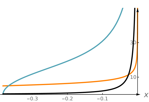
Figure 3: A solution with $t=-\frac{1}{4}$, $\sigma=-4$, $F_{0}=-\frac{4}{2\pi}$ , and $L=8$. The plotted functions are $e^{W}$(orange), $e^{\phi}$(black) and $e^{\lambda_{1}}$(turquoise). On the left ($x_{0}=-0.38$) the $S^{1}$ shrinks regularly, on the right ($x=0$) a diverging-dilaton O8 sits.

On these solutions we can compute the quantity $e^{5W-\phi}$ analytically and we obtain

$$e^{5W-\phi}=\left\{\begin{array}[]{l}F_{0}L^{6}\frac{\left(x^{3}-1\right)^{2}}{3x^{3}+\sigma x+6}\\ \\ F_{0}L^{6}\frac{(t-x^{3})(x^{3}-1)}{3x^{3}+\sigma x+3(t+1)}\end{array}\right.$$ (A.11)

so that in both cases

$$\lim_{x\rightarrow 0}\partial_{x}(5W-\phi)\propto\sigma\neq 0\;.$$ (A.12)

We see that generically this is non-zero, and hence satisfies the permissive boundary conditions (4.9), but not the restrictive ones (4.11).

References

- [1] G. W. Gibbons, “Aspects of Supergravity Theories,”. Lectures at San Feliu de Guixols, Spain, June, 1984.
- [2] B. de Wit, D. J. Smit, and N. D. Hari Dass, “Residual Supersymmetry of Compactified Supergravity,” Nucl. Phys. B283 (1987) 165.
- [3] J. M. Maldacena and C. Núñez, “Supergravity description of field theories on curved manifolds and a no-go theorem,” Int. J. Mod. Phys. A16 (2001) 822–855, hep-th/0007018.
- [4] S. Kachru, R. Kallosh, A. Linde, and S. P. Trivedi, “De Sitter vacua in string theory,” Phys. Rev. D68 (2003) 046005, hep-th/0301240.
- [5] V. Balasubramanian, P. Berglund, J. P. Conlon, and F. Quevedo, “Systematics of Moduli Stabilisation in Calabi–Yau Flux Compactifications,” JHEP 03 (2005) 007, hep-th/0502058.
- [6] E. Silverstein, “Simple de Sitter Solutions,” Phys. Rev. D77 (2008) 106006, 0712.1196.
- [7] C. Caviezel, P. Koerber, S. Körs, D. Lüst, T. Wrase, and M. Zagermann, “On the Cosmology of Type IIA Compactifications on -structure Manifolds,” JHEP 04 (2009) 010, 0812.3551.
- [8] U. H. Danielsson, P. Koerber, and T. Van Riet, “Universal de Sitter solutions at tree-level,” JHEP 05 (2010) 090, 1003.3590.
- [9] X. Dong, B. Horn, E. Silverstein, and G. Torroba, “Micromanaging de Sitter holography,” Class. Quant. Grav. 27 (2010) 245020, 1005.5403.
- [10] J. Blåbäck, U. H. Danielsson, D. Junghans, T. Van Riet, T. Wrase, and M. Zagermann, “The problematic backreaction of SUSY-breaking branes,” JHEP 1108 (2011) 105, 1105.4879.
- [11] I. Bena, M. Graña, and N. Halmagyi, “On the Existence of Meta-stable Vacua in Klebanov–Strassler,” JHEP 09 (2010) 087, 0912.3519.
- [12] T. Banks, “The Top Reasons Not to Believe in the Landscape,” 1208.5715.
- [13] S. Sethi, “Supersymmetry Breaking by Fluxes,” JHEP 10 (2018) 022, 1709.03554.
- [14] U. H. Danielsson and T. Van Riet, “What if string theory has no de Sitter vacua?,” Int. J. Mod. Phys. D27 (2018), no. 12, 1830007, 1804.01120.
- [15] G. Obied, H. Ooguri, L. Spodyneiko, and C. Vafa, “De Sitter Space and the Swampland,” 1806.08362.
- [16] D. Andriot, “On the de Sitter swampland criterion,” Phys. Lett. B785 (2018) 570–573, 1806.10999.
- [17] F. Denef, A. Hebecker, and T. Wrase, “de Sitter swampland conjecture and the Higgs potential,” Phys. Rev. D98 (2018), no. 8, 086004, 1807.06581.
- [18] S. K. Garg and C. Krishnan, “Bounds on Slow Roll and the de Sitter Swampland,” 1807.05193.
- [19] H. Ooguri, E. Palti, G. Shiu, and C. Vafa, “Distance and de Sitter Conjectures on the Swampland,” Phys. Lett. B788 (2019) 180–184, 1810.05506.
- [20] D. Andriot, “Open problems on classical de Sitter solutions,” Fortsch. Phys. 67 (2019), no. 7, 1900026, 1902.10093.
- [21] S. Kachru and S. P. Trivedi, “A comment on effective field theories of flux vacua,” Fortsch. Phys. 67 (2019), no. 1-2, 1800086, 1808.08971.
- [22] S. Das, S. S. Haque, and B. Underwood, “Constraints and horizons for de Sitter with extra dimensions,” Phys. Rev. D100 (2019), no. 4, 046013, 1905.05864.
- [23] C. Córdova, G. B. De Luca, and A. Tomasiello, “Classical de Sitter Solutions of Ten-Dimensional Supergravity,” Phys. Rev. Lett. 122 (2019), no. 9, 091601, 1812.04147.
- [24] N. Seiberg and E. Witten, “Gauge dynamics and compactification to three-dimensions,” in The mathematical beauty of physics: A memorial volume for Claude Itzykson. Proceedings, Conference, Saclay, France, June 5-7, 1996, pp. 333–366. 1996. hep-th/9607163.
- [25] A. Hanany and B. Pioline, “(Anti-)instantons and the Atiyah-Hitchin manifold,” JHEP 0007 (2000) 001, hep-th/0005160.
- [26] A. Passias, A. Rota, and A. Tomasiello, “Universal consistent truncation for 6d/7d gauge/gravity duals,” JHEP 10 (2015) 187, 1506.05462.
- [27] F. Apruzzi, M. Fazzi, D. Rosa, and A. Tomasiello, “All AdS7 solutions of type II supergravity,” JHEP 1404 (2014) 064, 1309.2949.
- [28] F. Apruzzi and M. Fazzi, “AdS7/CFT6 with orientifolds,” JHEP 01 (2018) 124, 1712.03235.
- [29] N. Cribiori and D. Junghans, “No classical (anti-)de Sitter solutions with O8-planes,” Phys. Lett. B793 (2019) 54–58, 1902.08209.
- [30] A. Passias, D. Prins, and A. Tomasiello, “A massive class of AdS4 IIA solutions,” JHEP 10 (2018) 071, 1805.03661.
- [31] A. Brandhuber and Y. Oz, “The D4–D8 brane system and five-dimensional fixed points,” Phys.Lett. B460 (1999) 307–312, hep-th/9905148.
- [32] I. Bah, A. Passias, and A. Tomasiello, “AdS5 compactifications with punctures in massive IIA supergravity,” JHEP 11 (2017) 050, 1704.07389.
- [33] G. Dibitetto, G. Lo Monaco, A. Passias, N. Petri, and A. Tomasiello, “AdS3 solutions with exceptional supersymmetry,” Fortsch. Phys. 66 (2018), no. 10, 1800060, 1807.06602.
- [34] G. Dibitetto and A. Passias, “AdS solutions from D0–F1–D8 intersections,” JHEP 10 (2018) 190, 1807.00555.
- [35] C. Córdova, G. B. De Luca, and A. Tomasiello, “AdS8 Solutions in Type II Supergravity,” 1811.06987.
- [36] A. Sen, “Orientifold limit of F-theory vacua,” Phys. Rev. D55 (1997) 7345–7349, hep-th/9702165.
- [37] G. W. Gibbons, G. T. Horowitz, and P. K. Townsend, “Higher dimensional resolution of dilatonic black hole singularities,” Class. Quant. Grav. 12 (1995) 297–318, hep-th/9410073.
- [38] E. Silverstein, “New de Sitter Solutions,” Plenary Talk at Strings, June 2013.
- [39] E. Witten, “Toroidal compactification without vector structure,” JHEP 02 (1998) 006, hep-th/9712028.
- [40] M. Bianchi, G. Pradisi, and A. Sagnotti, “Toroidal compactification and symmetry breaking in open string theories,” Nucl. Phys. B376 (1992) 365–386.
- [41] C. Angelantonj, M. Bianchi, G. Pradisi, A. Sagnotti, and Y. S. Stanev, “Comments on Gepner models and type I vacua in string theory,” Phys. Lett. B387 (1996) 743–749, hep-th/9607229.
- [42] F. Apruzzi, M. Fazzi, A. Passias, A. Rota, and A. Tomasiello, “Six-Dimensional Superconformal Theories and their Compactifications from Type IIA Supergravity,” Phys. Rev. Lett. 115 (2015), no. 6, 061601, 1502.06616.
- [43] S. Cremonesi and A. Tomasiello, “6d holographic anomaly match as a continuum limit,” JHEP 05 (2016) 031, 1512.02225.
- [44] A. Rota and A. Tomasiello, “AdS compactifications of AdS solutions in type II supergravity,” JHEP 07 (2015) 076, 1502.06622.
- [45] C. Córdova, T. T. Dumitrescu, and K. Intriligator, “Anomalies, Renormalization Group Flows, and the -Theorem in Six-Dimensional Theories,” 1506.03807.
- [46] F. F. Gautason, D. Junghans, and M. Zagermann, “Cosmological Constant, Near Brane Behavior and Singularities,” JHEP 1309 (2013) 123, 1301.5647.
- [47] G. B. De Luca. Work in Progress.
- [48] R. Steinbauer and J. A. Vickers, “The Use of generalised functions and distributions in general relativity,” Class. Quant. Grav. 23 (2006) R91–R114, gr-qc/0603078.
- [49] A. Passias and P. Richmond, “Perturbing AdS: linearised equations and spin-2 spectrum,” JHEP 07 (2018) 058, 1804.09728.
- [50] D. Andriot and D. Tsimpis, “Gravitational waves in warped compactifications,” 1911.01444.
- [51] N. Dorey, V. Khoze, M. P. Mattis, D. Tong, and S. Vandoren, “Instantons, three-dimensional gauge theory, and the Atiyah–Hitchin manifold,” Nucl. Phys. B502 (1997) hep-th/9703228.
- [52] M. Atiyah and N. J. Hitchin, “Low-Energy Scattering of Nonabelian Monopoles,” Phys.Lett. A107 (1985) 21–25.
- [53] F. Saracco, A. Tomasiello, and G. Torroba, “Topological resolution of gauge theory singularities,” Phys.Rev. D88 (2013) 045018, 1305.2929.
- [54] F. Saracco and A. Tomasiello, “Localized O6-plane solutions with Romans mass,” JHEP 1207 (2012) 077, 1201.5378.
- [55] B. Michel, E. Mintun, J. Polchinski, A. Puhm, and P. Saad, “Remarks on brane and antibrane dynamics,” JHEP 09 (2015) 021, 1412.5702.
- [56] H. Balasin and H. Nachbagauer, “The energy-momentum tensor of a black hole, or what curves the Schwarzschild geometry?,” Class. Quant. Grav. 10 (1993) 2271, gr-qc/9305009.
- [57] H. Balasin and H. Nachbagauer, “Distributional energy momentum tensor of the Kerr–Newman space-time family,” Class. Quant. Grav. 11 (1994) 1453–1462, gr-qc/9312028.
- [58] G. Compère and A. Fiorucci, “Advanced Lectures on General Relativity,” Lect. Notes Phys. 952 (2019) 150, 1801.07064.