Three-loop soft function for heavy-to-light quark decays

Abstract

We compute the 1-jettiness soft function for the decay of a heavy quark into a light quark jet plus colorless particles at three-loop order in soft-collinear effective theory. The 1-jettiness measurement fixes the total small light-cone momentum component of the soft radiation with respect to the jet direction. This soft function is a universal ingredient to the factorization of heavy-to-light quark decays in the limit of small 1-jettiness. Our three-loop result is required for resummation at the N³LL^′ level, e.g. near the endpoint in the photon energy spectrum of the $B\to X_{s}\gamma$ decay. It is also a necessary ingredient for future calculations of fully-differential heavy-to-light quark decay rates at N³LO using the $N$-jettiness subtraction method, e.g. for semileptonic top decays. Using our result for the soft anomalous dimension we confirm predictions on the universal infrared structure of QCD scattering amplitudes with a massive external quark at three loops.

1 Introduction

Heavy quark (bottom, top) decays are phenomenologically important Standard Model (SM) processes. A prominent example is the decay $b\to s\gamma$. In the SM it is loop-suppressed and represents a promising window to new physics. In particular, beyond SM interactions due to flavor changing neutral currents could add a measurable effect on the decay rate of $B\to X_{s}\gamma$ on top of the small SM background. In the phenomenologically relevant region of large photon energies the decay rate $\Gamma(B\to X_{s}\gamma)$ factorizes as Korchemsky:1994jb

$$\frac{\mathrm{d}\Gamma}{\mathrm{d}E_{\gamma}}=H(E_{\gamma},m_{b},\mu)\int\!\mathrm{d}\omega\,m_{b}\,J(m_{b}\,\omega,\mu)\,\mathcal{S}(\Delta-\omega,\mu)+{\mathcal{O}}\biggl{(}\frac{\Delta}{m_{b}},\frac{\Lambda_{\mathrm{QCD}}}{m_{b}}\biggr{)}\,,$$ (1)

where $\Delta=m_{b}-2E_{\gamma}$. Within soft-collinear effective theory (SCET) Bauer:2000ew ; Bauer:2000yr ; Bauer:2001ct ; Bauer:2001yt ; Bauer:2002nz ; Beneke:2002ph this factorization theorem was proven in ref. Bauer:2001yt . The hard function $H$ encodes the short distance (electroweak) interaction and its virtual quantum corrections at and beyond the hard scale $m_{b}\sim E_{\gamma}$. Explicit expressions up to two loops can be found in refs. Ligeti:2008ac ; Ali:2007sj . The jet function $J$ describes the collinear radiation in the final state jet initiated by the (massless) $s$ quark and is governed by the virtuality scale $\sqrt{m_{b}\Delta}$. In ref. Bruser:2018rad we computed the massless quark jet function to three-loop order (see also ref. Banerjee:2018ozf ). Finally, $\mathcal{S}$ denotes the $B$-meson shape function Neubert:1993um ; Bigi:1993ex which describes the physics at scales smaller or similar to $\Delta$. For $\Delta\gtrsim\Lambda_{\mathrm{QCD}}$ nonperturbative effects are sizable and one can further factorize $\mathcal{S}$ into a purely perturbative ‘heavy-to-light soft function’ $S_{\mathrm{hl}}$ and a nonperturbative shape function $F$ Ligeti:2008ac :

$$\mathcal{S}(\omega,\mu)=\int\!\mathrm{d}\omega^{\prime}\,S_{\mathrm{hl}}(\omega-\omega^{\prime},\mu)\,F(\omega^{\prime})\,,$$ (2)

with $\int\!\mathrm{d}\omega\,F(\omega)=1$. The soft function $S_{\mathrm{hl}}$ can be expressed as a partonic $b$-quark matrix element, see eq. (6), and was computed to two-loop order in ref. Becher:2005pd . The functions $J$, $S_{\mathrm{hl}}$, and $F$ vanish when their first argument is negative. This entails finite integration ranges in eqs. (1) and (2). The perturbative factorization functions $H$, $J$, and $S_{\mathrm{hl}}$ depend individually on the common renormalization scale $\mu$, while the total decay rate in eq. (1) is $\mu$ independent to the perturbative order one is working at. The renormalization group (RG) evolution of the hard, jet, and, soft functions is therefore not independent, but subject to a consistency relation (which will be relevant later). The combined RG running of the different functions to the common scale $\mu$ eventually resums large logarithms of the ratios between the hard, jet, and soft (matching) scales $\mu_{H}\sim m_{b}$, $\mu_{J}\sim\sqrt{m_{b}\Delta}$, and $\mu_{S}\sim\Delta$.

A factorization theorem analogous to eq. (1) also holds for the decay $B\to X_{u}\ell\bar{\nu}$. In particular the involved jet and shape functions are the same. The nonperturbative function $F$ can thus be obtained from a fit to experimental data for the differential spectrum of one or both decays, see e.g. ref. Bernlochner:2013gla , and then be used for theoretical predictions. For details we refer to ref. Ligeti:2008ac . The current state of the art for such predictions includes resummation at the primed next-to-next-to-leading logarithmic (NNLL^′) level Ligeti:2008ac ; Becher:2006pu , where the NNLL expression Neubert:2004dd is augmented with the next-to-next-to-leading order (NNLO) corrections to the factorization functions at their matching scales, i.e. to $H(\mu_{H}$), $J(\mu_{J})$, $S_{\mathrm{hl}}(\mu_{S})$. Still, the uncertainties from missing higher-order perturbative corrections represent a major contribution to the total error budget Bernlochner:2013gla .

In order to reach N³LL^′ accuracy of the decay rate in eq. (1) the three-loop corrections to the hard, jet, and soft, functions along with their anomalous dimensions are required. Our three-loop calculation of the jet function in ref. Bruser:2018rad represents a first step toward this goal. In the present paper we calculate the soft function $S_{\mathrm{hl}}$ at three loops, while the three-loop hard function is left for future work. We also give explicit expressions for all three-loop (noncusp) anomalous dimensions necessary for N³LL^(′) resummation in eq. (1).

Another possible application of our result is within the context of $N$-jettiness subtractions Boughezal:2015dva ; Gaunt:2015pea . In its simplest version the latter is an infrared (IR) slicing method which uses the observable $N$-jettiness $\mathcal{T}_{N}$ Stewart:2010tn as an auxiliary resolution variable for soft and collinear real emissions. It was employed amongst others to compute the fully-differential decay rate of the semileptonic top decay $t\to W^{+}(l^{+}\nu)b$ at NNLO in QCD Gao:2012ja . In this case the resolution variable is $\mathcal{T}_{1}$ (1-jettiness). For $\mathcal{T}_{1}<\mathcal{T}_{\mathrm{cut}}$ the decay rate is given by a factorization formula analogous to eq. (1), but with $\mathcal{S}=S_{\mathrm{hl}}$, provided that $\mathcal{T}_{\mathrm{cut}}$ is small enough to neglect ${\mathcal{O}}(\mathcal{T}_{\mathrm{cut}}/m_{t})$ power corrections at the desired precision. For $\mathcal{T}_{1}>\mathcal{T}_{\mathrm{cut}}$ there is at least one additional hard parton in the final state. On the other hand quantum corrections to this part of the decay rate are only needed at one order lower in the perturbative expansion. In case of the NNLO $t\to W^{+}(l^{+}\nu)b$ decay the $\mathcal{T}_{1}>\mathcal{T}_{\mathrm{cut}}$ piece can therefore be computed with standard (numerical) NLO technology. The soft function $S_{\mathrm{hl}}$ we calculate in the present paper equals the soft function in the 1-jettiness factorization theorem for any heavy-to-light quark decay. The new three-loop contribution is thus a necessary ingredient for future N³LO calculations of differential decay rates based on the $N$-jettiness method, not only for semileptonic top, but also any other heavy-to-light quark decay.

The outline of this paper is as follows. In sec. 2 we give four (slightly) different definitions of the heavy-to-light soft function $S_{\mathrm{hl}}$ and show their equivalence. We give details on our three-loop calculation based on one of these definitions in sec. 3. In sec. 4 we present our results for the renormalized soft function and its anomalous dimension. We also use the latter to check the universal infrared structure of QCD scattering amplitudes that have a massive quark leg. We briefly summarize our findings in sec. 5.

2 Definitions

The 1-jettiness soft function for heavy-to-light decays is defined by the vacuum matrix element

$$S_{\mathrm{hl}}(\omega):=\frac{1}{N_{c}}\operatorname{tr}\operatorname{\big{\langle}0\big{|}}\operatorname{\overline{T}}\Big{[}\big{(}X_{+}\big{)}^{\!\dagger}\!(0)\,Y_{-}(0)\Big{]}\,\delta(\omega-n\!\cdot\!\hat{p})\,\operatorname{T}\Big{[}\big{(}Y_{-}\big{)}^{\!\dagger}\!(0)\,X_{+}(0)\Big{]}\operatorname{\big{|}0\big{\rangle}}\,,$$ (3)

with the soft momentum operator $\hat{p}^{\mu}$ and the Wilson lines

$$X_{+}(x) =\mathrm{P}\exp\Big{[}ig\!\int_{-\infty}^{0}\!\!\!\mathrm{d}s\;v\!\cdot\!A(x+sv)\Big{]}\,,$$ (4)

$$Y_{-}(x) =\overline{\mathrm{P}}\exp\Big{[}-ig\!\int^{\infty}_{0}\!\!\mathrm{d}s\;n\!\cdot\!A(x+sn)\Big{]}\,,$$ (5)

where $A_{\mu}(x)\equiv A_{\mu}^{a}(x)T^{a}$ is the (ultra)soft SCET_(I) gluon field, $v_{\mu}$ is the heavy quark velocity ($v^{2}=1$), $n_{\mu}$ is the light-like jet direction ($n^{2}=0$) and $\mathrm{P}$ ($\overline{\mathrm{P}}$) denotes (anti-)path ordering of the $A_{\mu}$ including their $SU(N_{c})$ color generators $T^{a}$. The trace in eq. (3) is over color indices, and $\operatorname{T}[\ldots]$ and $\operatorname{\overline{T}}[\ldots]$ represent time- and anti-time-ordered products of the field operators $A_{\mu}^{a}(x)$, respectively. The argument $\omega$ of $S_{\mathrm{hl}}$ can be regarded as the (appropriately normalized) soft contribution to the 1-jettiness observable $\mathcal{T}_{1}$, cf. ref. Stewart:2010tn .

The soft function in eq. (3) equals the perturbative contribution to the shape function in eq. (2):

$$S_{\mathrm{hl}}(\omega)=\big{\langle}b_{v}\big{|}\overline{h}_{v}(0)\,\delta(\omega+in\!\cdot\!D)\,h_{v}(0)\big{|}b_{v}\big{\rangle}\,,$$ (6)

where averaging over color and spin of the external HQET $b$-quark states is understood, the latter are normalized such that $\langle b_{v}|\overline{h}_{v}(0)h_{v}(0)|b_{v}\rangle=1$, $h_{v}$ is the HQET heavy quark field with velocity $v$, and $D^{\mu}=\partial^{\mu}+igA^{\mu}(0)$. This $b$-quark matrix element was calculated to ${\mathcal{O}}(\alpha_{s})$ in refs. Bauer:2003pi ; Bosch:2004th and ${\mathcal{O}}(\alpha_{s}^{2})$ in ref. Becher:2005pd . The equivalence to eq. (3) can be seen as follows:

$$\big{\langle}b_{v}\big{|}\overline{h}_{v}(0)\,\delta(\omega+in\!\cdot\!D)\,h_{v}(0)\big{|}b_{v}\big{\rangle}$$

$$=\big{\langle}b_{v}\big{|}\overline{h}_{v}(0)\,Y_{-}(0)\,\delta(\omega+in\!\cdot\!\partial)\,\big{(}Y_{-}\big{)}^{\!\dagger}\!(0)\,h_{v}(0)\big{|}b_{v}\big{\rangle}$$ (7)

$$=\big{\langle}b_{v}\big{|}\operatorname{\overline{T}}\Big{[}\overline{h}_{v}(0)\,Y_{-}(0)\Big{]}\,\delta(\omega-n\!\cdot\!\hat{p})\,\operatorname{T}\Big{[}\big{(}Y_{-}\big{)}^{\!\dagger}\!(0)\,h_{v}(0)\Big{]}\big{|}b_{v}\big{\rangle}$$ (8)

$$=\big{\langle}b_{v}^{(0)}\big{|}\overline{h}_{v}^{(0)}(0)\operatorname{\overline{T}}\Big{[}\big{(}X_{+}\big{)}^{\!\dagger}\!(0)\,Y_{-}(0)\Big{]}\,\delta(\omega-n\!\cdot\!\hat{p})\,\operatorname{T}\Big{[}\big{(}Y_{-}\big{)}^{\!\dagger}\!(0)\,X_{+}(0)\Big{]}h_{v}^{(0)}(0)\big{|}b_{v}^{(0)}\big{\rangle}$$ (9)

$$=S_{\mathrm{hl}}(\omega)\,.$$ (10)

In eq. (8) we could introduce the $\operatorname{T}$ and $\operatorname{\overline{T}}$ symbols, because the field operators in $Y_{-}$ are already anti-time-ordered by default as a consequence of the anti-path-ordering, and Hermitian conjugation reverses the order. Similarly the $\operatorname{T}$ and $\operatorname{\overline{T}}$ symbols in eqs. (9) and (3) are in fact redundant, but kept for clarity. In eq. (9) we performed the HQET field redefinition

$$h_{v}(x)\to X_{+}(x)\,h_{v}^{(0)}(x)\,,$$ (11)

where the new (sterile) field $h_{v}^{(0)}$ does not interact with soft gluons anymore, see e.g. ref. Bauer:2001yt . Note that given the (anti)-time-ordering the external $b$-quark states should be interpreted as ‘in’ states, $|b_{v}\rangle=|b_{v},\mathrm{in}\rangle$, $\langle b_{v}|=\langle b_{v},\mathrm{in}|$. The LSZ reduction formula relates the asymptotic ‘in’/‘out’ $b$-quark states of the S-matrix element to weighted integrals over interpolating $\overline{h}_{v}(x)$/$h_{v}(x)$ field operators acting on the vacuum at macroscopically large negative/positive times. Performing the field redefinition in eq. (11) one also has to take into account factors of $X_{+}$ from these interpolating fields. For the ‘in’ states this factor is trivial and we can effectively replace Arnesen:2005nk

$$\big{|}b_{v},\mathrm{in}\big{\rangle}_{i}\to\Big{[}\big{(}X_{+}\big{)}^{\!\dagger}\!(t\!=\!-\infty,\vec{x}=0)\Big{]}_{ji}\,\big{|}b_{v}^{(0)},\mathrm{in}\big{\rangle}_{j}=\big{|}b_{v}^{(0)},\mathrm{in}\big{\rangle}_{i}\;,$$ (12)

where $i$, $j$ are color indices in the fundamental representation. Here and in the following we assume the $b$ quark to be at rest, i.e. $v^{\mu}=(1,\vec{0})$ for simplicity. The spatial position $\vec{x}$ of the endpoint of the Wilson line $X_{+}$ in eq. (12) is fixed by the position of the field operator, here $h_{v}(0)$, acting on the asymptotic state, because $\langle 0|h_{v}(x)\overline{h}_{v}(y)|0\rangle\propto\delta^{(3)}(\vec{x}-\vec{y})$. Finally, the sterile HQET quark field operators in eq. (9) annihilate the sterile external quarks and the color averaging implicit in the $b$-quark matrix elements translates to $1/N_{c}$ times the color trace in eq. (3).

For the actual calculation of the soft function it is convenient to express it as the imaginary part (discontinuity) of a ($1\to 1$) ‘forward scattering’ matrix element. Starting from eq. (8) and inserting a complete set of states we have

$$S_{\mathrm{hl}}(\omega)=\sum\!\!\!\!\!\!\!\!\int\limits_{Z}\;\delta(\omega-p_{Z}^{+})\,\Big{|}\big{\langle}Z\big{|}\operatorname{T}\Big{[}\big{(}Y_{-}\big{)}^{\!\dagger}\!(0)\,h_{v}(0)\Big{]}\big{|}b_{v}\big{\rangle}\Big{|}^{2}$$

$$\quad=\mathrm{Im}\bigg{[}\,i\sum\!\!\!\!\!\!\!\!\int\limits_{Z}\,\int_{-\infty}^{\infty}\!\frac{\mathrm{d}s}{2\pi}\,\frac{i}{s+i0}\;\delta\Big{(}\frac{\omega}{2}-\frac{p_{Z}^{+}}{2}-s\Big{)}\,\Big{|}\big{\langle}Z\big{|}\big{(}Y_{-}\big{)}^{\!\dagger}\!(0)\,h_{v}(0)\big{|}b_{v}\big{\rangle}\Big{|}^{2}\;\bigg{]}$$ (13)

$$\quad=\mathrm{Im}\bigg{[}\,i\sum\!\!\!\!\!\!\!\!\int\limits_{Z}\,\int_{-\infty}^{\infty}\!\frac{\mathrm{d}x^{-}}{2\pi}\,e^{\frac{i}{2}\omega x^{-}}\!\!\int_{-\infty}^{\infty}\!\frac{\mathrm{d}s}{2\pi}\,\frac{ie^{-isx^{-}}}{s+i0}$$

$$\qquad\qquad\times\big{\langle}b_{v}\big{|}e^{\frac{i}{2}\hat{p}^{+}x^{-}}\,\overline{h}_{v}(0)\,Y_{-}(0)\,e^{-\frac{i}{2}\hat{p}^{+}x^{-}}\big{|}Z\big{\rangle}\big{\langle}Z\big{|}\big{(}Y_{-}\big{)}^{\!\dagger}\!(0)\,h_{v}(0)\big{|}b_{v}\big{\rangle}\bigg{]}$$ (14)

$$\quad=\mathrm{Im}\bigg{[}\,i\int_{-\infty}^{\infty}\!\frac{\mathrm{d}x^{-}}{2\pi}\,e^{\frac{i}{2}\omega x^{-}}\theta(x^{-})\big{\langle}b_{v}\big{|}\overline{h}_{v}\big{(}x^{-}{\textstyle\frac{n}{2}}\big{)}\,Y_{-}\big{(}x^{-}{\textstyle\frac{n}{2}}\big{)}\,\big{(}Y_{-}\big{)}^{\!\dagger}\!(0)\,h_{v}(0)\big{|}b_{v}\big{\rangle}\bigg{]}$$ (15)

$$\quad=\mathrm{Im}\bigg{[}\,i\int_{0}^{\infty}\!\frac{\mathrm{d}x^{-}}{2\pi}\,e^{\frac{i}{2}\omega x^{-}}\big{\langle}b_{v}\big{|}\operatorname{T}\Big{[}\overline{h}_{v}\big{(}x^{-}{\textstyle\frac{n}{2}}\big{)}\,\mathrm{P}\exp\Big{[}ig\!\int_{0}^{x^{-}\!/2}\!\!\mathrm{d}s\;n\!\cdot\!A(sn)\Big{]}\,h_{v}(0)\Big{]}\big{|}b_{v}\big{\rangle}\bigg{]}\,.$$ (16)

Here we use the usual light-cone (Sudakov) decomposition of four vectors: $a^{\mu}=a^{-}n^{\mu}/2+a^{+}\bar{n}^{\mu}/2+a^{\mu}_{\perp}$ with $n^{2}=\bar{n}^{2}=0$ and $\bar{n}\cdot n=2$. Note that the momentum operator $\hat{p}^{+}$ acting to the left on the external HQET state in eq. (14) vanishes, because the external heavy quarks are onshell and therefore have zero residual (soft) four-momentum. While for space-like distance $x^{2}<0$ the field operators commute, the theta function $\theta(x^{-})$ in eq. (15) implies $t>0$ for time-like distances $x^{2}>0$. After combining the two Wilson lines using their unitarity property the remaining field operators are therefore automatically time-ordered. To make this manifest we explicitly inserted the $\operatorname{T}$ symbol in eq. (16).

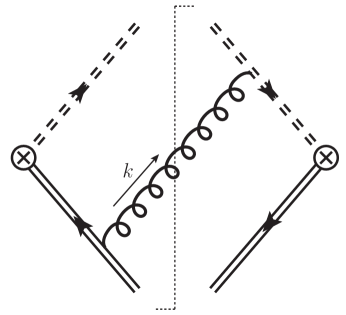
Figure 1: The cut diagram on the left hand side represents one ${\mathcal{O}}(\alpha_{s}$) contribution to $S_{\mathrm{hl}}$ in eq. (3). The phase space integration of the soft gluon (with outgoing momentum $k^{\mu}$) crossing the final state cut is restricted by the measurement function $\delta(\omega-n\!\cdot\!\hat{p})$. The equivalent contribution to the expression in eq. (18) comes from the loop diagram on the right hand side, where the external lightcone momentum $\omega$ is routed through the light-like Wilson line as indicated. Here and in the following dashed double lines represent light-like Wilson lines ($Y$) and solid double lines represent time-like Wilson lines ($X$). The arrows on the Wilson lines indicate the fermion flow of the respective original quarks, which coincides with the direction of the path as well as the time ordering in this case.

We can now again perform the field redefinition in eq. (11). This time, however, the time ordering in eq. (16) implies that $|b_{v}\rangle=|b_{v},\mathrm{in}\rangle$ and $\langle b_{v}|=\langle b_{v},\mathrm{out}|$. In contrast to eq. (12) the field redefinition now induces a non-trivial factor from the interpolating fields generating the ‘out’ state Arnesen:2005nk :

$${\phantom{\rangle}}_{i}\big{\langle}b_{v},\mathrm{out}\big{|}\to{\phantom{\rangle}}_{j}\big{\langle}b_{v}^{(0)},\mathrm{out}\big{|}\Big{[}X_{+}(t\!=\!+\infty,x^{-}\textstyle\frac{\vec{n}}{2})\Big{]}_{ij}={\phantom{\rangle}}_{j}\big{\langle}b_{v}^{(0)},\mathrm{out}\big{|}\Big{[}\big{(}X_{-}\big{)}^{\!\dagger}\!\big{(}x^{-}{\textstyle\frac{n}{2}}\big{)}\,X_{+}\big{(}x^{-}{\textstyle\frac{n}{2}}\big{)}\Big{]}_{ij}\;.$$ (17)

Using $r=x^{-}/2$ as integration variable we thus obtain

$$S_{\mathrm{hl}}(\omega)=\mathrm{Im}\bigg{[}\,\frac{i}{\pi}\,\frac{1}{N_{c}}\operatorname{tr}\int_{0}^{\infty}\!\!\mathrm{d}r\,e^{i\omega r}\operatorname{\big{\langle}0\big{|}}\operatorname{T}\Big{[}\big{(}X_{-}\big{)}^{\!\dagger}\!(rn)\,\mathrm{P}\exp\Big{[}ig\!\int_{0}^{r}\!\!\mathrm{d}s\;n\!\cdot\!A(sn)\Big{]}\,X_{+}(0)\Big{]}\operatorname{\big{|}0\big{\rangle}}\bigg{]}\,.$$ (18)

In this expression the time-like Wilson lines extend from $t=-\infty$ to $t=0$ (incoming) and from $t=r$ to $t=+\infty$ (outgoing), respectively. The light-like Wilson line connects the points $0$ and $rn^{\mu}$. The Wilson line correlator in eq. (18) can be straightforwardly evaluated in terms of (momentum-space) Feynman diagrams using the usual Feynman rules for Wilson lines in QCD. The equivalence of eqs. (3) and (18) is illustrated on the diagrammatic level at one loop in fig. 1. In fig. 2 we show some examples of corresponding three-loop diagrams. At ${\mathcal{O}}(g^{0})$ (tree level) $S_{\mathrm{hl}}$ is, according to eq. (18), proportional to the discontinuity of a single light-like Wilson line propagator with soft light-cone momentum $\omega$:

$$S_{\mathrm{hl}}^{(0)}(\omega)=\mathrm{Im}\bigg{[}\,\frac{i}{\pi}\,\int_{-\infty}^{\infty}\!\!\mathrm{d}r\,e^{i\omega r}\theta(r)\bigg{]}=\mathrm{Im}\bigg{[}\,\frac{i}{\pi}\,\frac{i}{\omega+i0}\,\bigg{]}=\delta(\omega)\,.$$ (19)

To conclude this section we comment on the relation of $S_{\mathrm{hl}}$ to the analogous 1-jettiness soft functions where one or both Wilson lines in eq. (3) are changed from incoming to outgoing or vice versa. In the underlying full QCD processes the external heavy and light quark lines are correspondingly crossed from initial to final state or vice versa. Some of these soft functions are e.g. relevant for $s$- and $t$-channel single top production as well as charm production in deep-inelastic neutrino scattering (‘light-to-heavy DIS’). For state-of-the-art fully-differential NNLO predictions we refer to ref. Liu:2018gxa , refs. Berger:2016oht ; Berger:2017zof , and ref. Berger:2016inr , respectively. The soft function for the light-to-heavy DIS process is for instance simply given by interchanging $X\leftrightarrow Y$ (i.e. $v^{\mu}\leftrightarrow n^{\mu}$ in the Wilson lines) in eq. (3). Up to two loops the soft functions for the crossed processes can be shown to equal $S_{\mathrm{hl}}$ as defined in eq. (3) in analogy to the massless case Kang:2015moa . Unfortunately there is, to the best of our knowledge, no simple argument why this equality should hold at three loops and beyond, not even between heavy-to-light decay and light-to-heavy DIS soft functions. A dedicated three-loop analysis along the lines of ref. Kang:2015moa would require to derive the analytic structure for the relevant two-loop single-emission and one-loop double-emission heavy-light soft currents, which is beyond the scope of this work.

3 Calculation

Figure 2: Sample Feynman diagrams contributing to $S_{\mathrm{hl}}$ at N³LO. Time-like Wilson lines, light-like Wilson lines, gluons, and light fermions are represented by solid double lines, dashed double lines, curly lines, and solid lines, respectively. The direction of the Wilson lines and the prescription for the routing of the external momentum $\omega$ are the same as in the one-loop diagram on the right of fig. 1.

Our three-loop calculation of the soft function $S_{\mathrm{hl}}$ is based on the definition in eq. (18) and performed very much along the lines of our jet function calculation in ref. Bruser:2018rad , to which we refer for more details. We work in general covariant gauge with gauge parameter $\xi$, where $\xi=0$ corresponds to Feynman gauge. Ultraviolet (UV) and (intermediate) IR divergences are regulated with dimensional regularization ($d=4-2\epsilon$).

We use qgraf Nogueira:1991ex to generate all relevant three-loop (propagator-type) Feynman graphs with one internal light-like and two external time-like Wilson lines (one incoming, one outgoing), like the ones in fig. 2. The diagrams are further processed by an in-house Mathematica code which assigns the corresponding Feynman rules and performs the necessary Dirac, Lorentz and color algebra. After that the diagrams are given by linear combinations of scalar Feynman integrals. These integrals can then be mapped onto 16 integral topologies with twelve linearly independent linear and quadratic propagators. The associated 16 integral families contain integrals with integer propagator powers ranging from minus three to plus five. The mapping of Feynman integrals onto the different topologies requires numerous multivariate partial fraction operations on products of linear Wilson line propagators followed by suitable shifts of the loop momenta. In order to automatize the extensive partial fractioning we implemented the algorithm outlined in ref. Pak:2011xt in our code.

Next, we perform the integration-by-parts (IBP) reduction Chetyrkin:1981qh of the integrals in each of the 16 families to a set of master integrals (MIs) using the public program FIRE5 Smirnov:2014hma . We then identify pairs of equal MIs of different families that are related by shifts of their loop momenta. The resulting total set of MIs across the 16 families still turns out to be redundant. We find 14 additional relations involving at least three MIs of different families due to partial fraction identities among their linear propagators. Finally, the three-loop contribution to the matrix element in eq. (18) can be expressed as a linear combination of 45 MIs belonging to nine different integral families. At this point we already notice that the gauge parameter $\xi$ manifestly cancels out in the sum of all diagrams indicating the correctness of our setup. The 45 contributing MIs can be cast into the form

$$G(\vec{a},\vec{b},\vec{c}\,)=\bigl{(}i\pi^{\frac{d}{2}}\bigr{)}^{-3}\!\int\!\!\frac{\mathrm{d}^{d}k_{1}\,\mathrm{d}^{d}k_{2}\,\mathrm{d}^{d}k_{3}}{{\mathcal{D}}_{1}^{a_{1}}{\mathcal{D}}_{2}^{a_{2}}{\mathcal{D}}_{3}^{a_{3}}{\mathcal{D}}_{4}^{a_{4}}{\mathcal{D}}_{5}^{a_{5}}{\mathcal{D}}_{6}^{a_{6}}{\mathcal{D}}_{7}^{b_{1}}{\mathcal{D}}_{8}^{b_{2}}{\mathcal{D}}_{9}^{b_{3}}{\mathcal{D}}_{10}^{b_{4}}{\mathcal{D}}_{11}^{b_{5}}{\mathcal{D}}_{12}^{c_{1}}{\mathcal{D}}_{13}^{c_{2}}{\mathcal{D}}_{14}^{c_{3}}{\mathcal{D}}_{15}^{c_{4}}{\mathcal{D}}_{16}^{c_{5}}}$$ (20)

with the following (linearly-dependent) propagator denominators

$${\mathcal{D}}_{1}=-k_{1}^{2}\,, \!\!{\mathcal{D}}_{2}=-k_{2}^{2}\,, \!\!{\mathcal{D}}_{3}=-k_{3}^{2}\,, \!\!{\mathcal{D}}_{4}=-(k_{1}-k_{2})^{2}\,,$$

$${\mathcal{D}}_{5}=-(k_{2}-k_{3})^{2}\,, \!\!{\mathcal{D}}_{6}=-(k_{3}-k_{1})^{2}\,, \!\!{\mathcal{D}}_{7}=-v\!\cdot\!k_{1}\,, \!\!{\mathcal{D}}_{8}=-v\!\cdot\!k_{2}\,,$$

$${\mathcal{D}}_{9}=-v\!\cdot\!k_{3}\,, \!\!{\mathcal{D}}_{10}=-v\!\cdot\!(k_{1}-k_{3})\,, \!\!{\mathcal{D}}_{11}=-v\!\cdot\!(k_{2}-k_{3})\,, \!\!{\mathcal{D}}_{12}=-n\!\cdot\!k_{1}-\omega\,,$$

$${\mathcal{D}}_{13}=-n\!\cdot\!k_{2}-\omega\,, \!\!{\mathcal{D}}_{14}=-n\!\cdot\!k_{3}-\omega\,, \!\!{\mathcal{D}}_{15}=-n\!\cdot\!(k_{1}-k_{3})-\omega\,, \!\!{\mathcal{D}}_{16}=-n\!\cdot\!(k_{2}-k_{3})-\omega\,,$$ (21)

where the usual (causal) ‘$-i0$’ prescription, i.e. ${\mathcal{D}}_{i}\to{\mathcal{D}}_{i}-i0$, is understood. The nine integral families containing the 45 MIs are defined by their maximal topologies with twelve linearly independent ${\mathcal{D}}_{i}$. These topologies are determined by restricting the propagator powers in eq. (20), for instance by

$$\text{topology 1:}\quad b_{4},b_{5},c_{4},c_{5}=0\,, \text{topology 2:}\quad b_{3},b_{5},c_{4},c_{5}=0\,,$$

$$\text{topology 3:}\quad b_{4},b_{5},c_{3},c_{4}=0\,, \text{topology 4:}\quad b_{3},b_{4},c_{3},c_{4}=0\,,$$

$$\text{topology 5:}\quad b_{2},b_{3},c_{4},c_{5}=0\,, \text{topology 6:}\quad b_{3},b_{4},c_{2},c_{4}=0\,,$$

$$\text{topology 7:}\quad b_{4},b_{5},c_{2},c_{4}=0\,, \text{topology 8:}\quad b_{3},b_{5},c_{3},c_{4}=0\,,$$

$$\text{topology 9:}\quad b_{3},b_{4},c_{1},c_{5}=0\,.$$ (22)

From the scaling properties of the integrand in eq. (20) for general time-like vector $v^{\mu}$ and light-like vector $n^{\mu}$ we conclude

$$G(\vec{a},\vec{b},\vec{c}\,)=\big{(}v^{2}\big{)}^{\frac{3}{2}d-A-B}(n\!\cdot\!v)^{2A+B-3d}(-\omega-i0)^{3d-2A-B-C}I(\vec{a},\vec{b},\vec{c},\epsilon)$$ (23)

with $A=\sum_{i}a_{i}$, $B=\sum_{i}b_{i}$, and $C=\sum_{i}c_{i}$. The dependence on the external kinematics thus totally factors out and we are left to compute the dimensionless function $I(\vec{a},\vec{b},\vec{c},\epsilon)$ as an expansion in $\epsilon$. For the case of heavy-to-light decays calculated in the rest frame of the heavy quark we have $v^{2}=n\!\cdot\!v=1$ by definition. For convenience we set $\omega=-1$ during the calculation of the MIs and restore their $\omega$ dependence later. Twelve MIs are simple enough to be evaluated by direct integrations over the associated Feynman parameters in $d=4-2\epsilon$ dimensions. The results involve hypergeometric and gamma functions and are expanded in $\epsilon$ with the help of the Mathematica package HypExp2 Huber:2007dx .

To solve the remaining 33 MIs we proceed in the same way as for our jet function calculation in ref. Bruser:2018rad . The method was inspired by refs. Panzer:2014gra ; vonManteuffel:2014qoa ; vonManteuffel:2015gxa . The key idea is to express the 33 MIs as a linear combination of quasi-finite integrals and known MIs. Quasi-finite integrals are free of (endpoint) divergences from the integrations in the Feynman parameter representation (at the Euclidean point $\omega=-1$) for some (even) integer dimension. Starting from a given MI in $d=4-2\epsilon$ one can construct a corresponding quasi-finite integral by raising the spacetime dimension by an even number and/or increasing appropriate propagator powers by integer amounts. The former decreases (increases) the degree of IR (UV) divergence, whereas the latter decreases (but not necessarily increases) the degree of UV (IR) divergence. To systematically identify suitable quasi-finite integrals we employ the dedicated algorithm implemented in the public program Reduze2 vonManteuffel:2012np . For our purposes we find 18 integrals that are quasi-finite in $4-2\epsilon$ and 15 integrals that are quasi-finite in $6-2\epsilon$ dimensions. To compute them in the respective dimension we first expand their nonsingular integrands in the Feynman parameter representation to high enough order in $\epsilon$. We then perform the integrations with the help of HyperInt Panzer:2014caa , a powerful computer algebra package for the analytical evaluation of convergent linearly reducible (Feynman) integrals in terms of multiple polylogarithms. The quasi-finite integrals (in their respective dimension) are related to the original MIs (in $d=4-2\epsilon$) by dimensional recurrence Tarasov:1996br ; Lee:2009dh ; Lee:2010wea and IBP reduction. To determine the relevant dimensional recurrence relations between integrals in $d$ and $d+2$ dimensions we use the public code LiteRed Lee:2012cn ; Lee:2013mka . Our choice of the 33 quasi-finite integrals is such that their results together with the 12 already computed MIs uniquely determine the remaining 33 MIs. We successfully verified all analytic expressions for the MIs obtained in this way numerically using the sector decomposition program FIESTA4 Smirnov:2015mct . Finally we insert the results for the 45 MIs in the IBP reduced expression for each three-loop Feynman diagram contributing to $S_{\mathrm{hl}}$ and expand to the required order in $\epsilon$, see below. We also repeated the calculation for the relevant lower-order graphs using the same setup.

4 Results

After computing the relevant Feynman diagrams as described in the previous section we take their imaginary part according to eq. (18) using

$$\mathrm{Im}\bigg{[}(-\omega-i0)^{-1-a\epsilon}\bigg{]} =-\sin(\pi a\epsilon)\,\theta(\omega)\,\omega^{-1-a\epsilon}\,.$$ (24)

Adding the contributions of all diagrams (including the lower-order ones) we obtain the bare soft function

$$S^{\mathrm{bare}}_{\mathrm{hl}}(\omega)={} 1+\frac{\alpha_{s}^{\mathrm{bare}}}{4\pi}\,\theta(\omega)\,\omega^{-1-2\epsilon}\,C_{F}\,K_{F}$$

$$+\bigg{(}\frac{\alpha_{s}^{\mathrm{bare}}}{4\pi}\bigg{)}^{\!2}\theta(\omega)\,\omega^{-1-4\epsilon}\,\bigg{(}C_{F}^{2}\,K_{FF}+C_{F}C_{A}\,K_{FA}+C_{F}n_{f}T_{F}\,K_{Ff}\bigg{)}$$

$$+\bigg{(}\frac{\alpha_{s}^{\mathrm{bare}}}{4\pi}\bigg{)}^{\!3}\theta(\omega)\,\omega^{-1-6\epsilon}\,\bigg{(}C_{F}^{3}\,K_{FFF}+C_{F}^{2}C_{A}\,K_{FFA}+C_{F}C_{A}^{2}\,K_{FAA}$$

$$\qquad+C_{F}^{2}n_{f}T_{F}\,K_{FFf}+C_{F}C_{A}n_{f}T_{F}\,K_{FAf}+C_{F}(n_{f}T_{F})^{2}\,K_{Fff}\bigg{)}+{\mathcal{O}}(\alpha_{s}^{4})$$ (25)

in terms of the bare coupling $\alpha_{s}^{\mathrm{bare}}=Z_{\alpha}\mu^{2\epsilon}\alpha_{s}$ with $n_{f}$ being the number of light (massless) quark flavours. The color constants of the $SU(N_{c})$ gauge group are $C_{A}=N_{c}$, $C_{F}=(N_{c}^{2}-1)/(2N_{c})$, and $T_{F}=1/2$. The coefficients $K_{X}$ of each color structure are given in app. B. For illustration we show in fig. 2 for each of the six three-loop $K_{X}$ coefficients one sample Feynman diagram (arranged in the corresponding order) that contributes to it. Throughout this work we employ the ${\overline{\rm MS}}$ renormalization scheme. The relevant terms of the strong coupling renormalization factor $Z_{\alpha}$ are

$$Z_{\alpha}=1+\frac{\alpha_{s}}{4\pi}\left(-\frac{\beta_{0}}{\epsilon}\right)+\left(\frac{\alpha_{s}}{4\pi}\right)^{2}\left(\frac{\beta_{0}^{2}}{\epsilon^{2}}-\frac{\beta_{1}}{2\epsilon}\right)+{\cal O}\left(\alpha_{s}^{3}\right)$$ (26)

with

$$\beta_{0}=\frac{11}{3}C_{A}-\frac{4}{3}T_{F}n_{f}\,,\qquad\beta_{1}=\frac{34}{3}C_{A}^{2}-\frac{20}{3}C_{A}n_{f}T_{F}-4C_{F}n_{f}T_{F}\,.$$ (27)

For the $\epsilon$ expansion of eq. (25) we employ the distributional identity

$$\mu^{a\epsilon}\,\theta(\omega)\,\omega^{-1-a\epsilon} =-\frac{\delta(\omega)}{a\epsilon}+\sum_{n=0}^{\infty}\frac{(-a\epsilon)^{n}}{n!}\frac{1}{\mu}{\mathcal{L}}_{n}\bigg{(}\frac{\omega}{\mu}\bigg{)}$$ (28)

with the usual plus distributions defined as

$${\mathcal{L}}_{n}(x) =\biggl{[}\frac{\theta(x)\ln^{n}\!x}{x}\biggr{]}_{+}\!\!=\lim_{\epsilon\to 0}\frac{\mathrm{d}}{\mathrm{d}x}\biggl{[}\theta(x-\epsilon)\frac{\ln^{n+1}x}{n+1}\biggr{]}\,.$$ (29)

The bare and renormalized soft functions are related by

$$S_{\mathrm{hl}}^{\mathrm{bare}}(\omega) =Z^{S}(\omega,\mu)\otimes S_{\mathrm{hl}}(\omega,\mu)\,,$$ (30)

where the $\otimes$ symbol denotes a convolution of the type

$$A(\omega)\otimes B(\omega)\equiv\int\!\mathrm{d}\omega^{\prime}\,A^{i}(\omega-\omega^{\prime})\,B(\omega^{\prime})\,.$$ (31)

Convolutions among the plus distributions ${\mathcal{L}}_{n}$ take the form

$${\mathcal{L}}_{m}(\omega)\otimes{\mathcal{L}}_{n}(\omega)=V_{-1}^{mn}\,\delta(\omega)+\sum_{k=0}^{m+n+1}V_{k}^{mn}\,{\mathcal{L}}_{k}(\omega)\,.$$ (32)

A generic expression for $V_{k}^{mn}$ can be found in ref. Ligeti:2008ac .

4.1 Anomalous Dimension

The RGE of our 1-jettiness soft function reads

$$\mu\frac{\mathrm{d}}{\mathrm{d}\mu}S_{\mathrm{hl}}(\omega,\mu) =\Gamma^{S}(\omega,\mu)\otimes S_{\mathrm{hl}}(\omega,\mu)\,,$$ (33)

with the anomalous dimension

$$\Gamma^{S}(\omega,\mu) =-\big{[}Z^{S}(\omega,\mu)\big{]}^{-1}\otimes\mu\frac{\mathrm{d}}{\mathrm{d}\mu}Z^{S}(\omega,\mu)$$ (34)

$$=2\Gamma^{q}_{\mathrm{cusp}}(\alpha_{s})\,\frac{1}{\mu}{\mathcal{L}}_{0}\bigg{(}\frac{\omega}{\mu}\bigg{)}+\gamma^{S}(\alpha_{s})\,\delta(\omega)\,.$$ (35)

For the loop expansion of the anomalous dimensions we adopt the notation

$$\Gamma^{q}_{\mathrm{cusp}}(\alpha_{s}) =\sum_{n=0}^{\infty}\Gamma^{q}_{n}\left(\frac{\alpha_{s}}{4\pi}\right)^{\!n+1}\,,\qquad\gamma^{S}(\alpha_{s})=\sum_{n=0}^{\infty}\gamma^{S}_{n}\left(\frac{\alpha_{s}}{4\pi}\right)^{\!n+1}\,.$$ (36)

With the soft renormalization factor $Z^{S}$ determined from our bare results in eq. (34) we obtain

$$\gamma^{S}_{0}={} 4C_{F}\,,$$ (37)

$$\gamma^{S}_{1}={} C_{F}\bigg{[}C_{A}\bigg{(}36\zeta_{3}-\frac{220}{27}-\frac{\pi^{2}}{9}\bigg{)}-n_{f}T_{F}\bigg{(}\frac{16}{27}+\frac{4\pi^{2}}{9}\bigg{)}\bigg{]}\,,$$ (38)

$$\gamma^{S}_{2}={} C_{F}\bigg{[}C_{A}^{2}\bigg{(}\frac{5428\zeta_{3}}{9}-\frac{64\pi^{2}\zeta_{3}}{9}-264\zeta_{5}-\frac{81215}{729}+\frac{853\pi^{2}}{243}-\frac{44\pi^{4}}{45}\bigg{)}$$ (39)

$$\quad+C_{A}n_{f}T_{F}\bigg{(}-\frac{4432\zeta_{3}}{27}+\frac{4460}{729}-\frac{1388\pi^{2}}{243}+\frac{16\pi^{4}}{15}\bigg{)}$$

$$\quad+C_{F}n_{f}T_{F}\bigg{(}-\frac{32\zeta_{3}}{9}+\frac{1442}{27}-\frac{4\pi^{2}}{3}-\frac{16\pi^{4}}{45}\bigg{)}+(n_{f}T_{F})^{2}\bigg{(}-\frac{448\zeta_{3}}{27}+\frac{6592}{729}+\frac{80\pi^{2}}{81}\bigg{)}\bigg{]}\,,$$

in addition to the known terms of the cusp anomalous dimension given in app. A. The one- and two-loop results in eqs. (37) and (38) agree with those in ref. Becher:2005pd (after adapting to their conventions). In the following we relate the soft anomalous dimension to corresponding collinear and hard anomalous dimensions in SCET factorization in order to verify our results. As we will see $\gamma^{S}_{2}$ can thus also be determined indirectly, i.e. without a dedicated three-loop calculation, using known results. However, to the best of our knowledge, the explicit expression in eq. (39) has not been given in the literature so far.

The anomalous dimension associated with the virtual IR singularities due to strong interactions among onshell partons in a squared QCD scattering amplitude can be understood as the anomalous dimension of a corresponding hard function in SCET. It is therefore intrinsically tied to the UV divergences of soft and collinear operator matrix elements in SCET by RG consistency. The generic all-order structure of the anomalous dimension for QCD amplitudes involving massive quarks was derived in ref. Becher:2009kw . For the heavy-to-light decay with one massless and one massive external quark the it is given by

$$\Gamma_{\mathrm{hl}}=-\Gamma^{q}_{\mathrm{cusp}}(\alpha_{s})\ln\frac{\mu}{2v\cdot p}+\gamma^{q}+\gamma^{Q}\,,$$ (40)

where $p$ is the (outgoing) four-momentum of the massless quark ($p^{2}=0$, $v\cdot p=m_{b}/2$) and $\Gamma^{q}_{\mathrm{cusp}}(\alpha_{s})$ is the light-like cusp anomalous dimension in the fundamental representation of $SU(N_{c})$. The noncusp anomalous dimensions $\gamma^{q}$ and $\gamma^{Q}$ are associated with each massless and massive external quark, respectively. They accordingly contribute to the anomalous dimension of any QCD scattering amplitude with multiple quark legs Becher:2009kw and are in that sense universal. The renormalized SCET hard function $H_{\mathrm{hl}}$ corresponds to the finite part of the respective QCD amplitude squared, i.e. where all IR and UV divergences have been subtracted. We thus have

$$\mu\frac{\mathrm{d}}{\mathrm{d}\mu}H_{\mathrm{hl}}=2\Gamma_{\mathrm{hl}}H_{\mathrm{hl}}\,.$$ (41)

For the QCD amplitude with two external heavy quarks (one outgoing, one incoming, where $p_{i}^{2}=m_{i}^{2}$, $p_{1}\!\cdot p_{2}>0$) the (hard) anomalous dimension reads

$$\Gamma_{\mathrm{hh}}=\Gamma^{Q}_{\mathrm{cusp}}(\beta,\alpha_{s})+2\gamma^{Q}\,.$$ (42)

Here the angle-dependent cusp anomalous dimension $\Gamma^{Q}_{\mathrm{cusp}}(\beta,\alpha_{s})$ with (Minkowskian) cusp angle $\beta=\mathrm{arccosh}(\frac{p_{1}\!\cdot p_{2}}{m_{1}m_{2}})$ is defined such that in the large angle expansion,

$$\Gamma^{Q}_{\mathrm{cusp}}(\beta,\alpha_{s})=\Gamma^{q}_{\mathrm{cusp}}(\alpha_{s})\,\beta+{\mathcal{O}}\biggl{(}\frac{1}{\beta}\biggr{)}\,,$$ (43)

there is no ${\mathcal{O}}(\beta^{0})$ term. As the large angle limit corresponds to the limit where the mass of one or both of the quarks vanishes it is not surprising that the coefficient of the leading term in eq. (43) equals the light-like cusp anomalous dimension Korchemsky:1985xj ; Korchemsky:1991zp .

For completeness and comparison we also recall the corresponding anomalous dimension for a QCD amplitude with two massless quarks ($p_{i}^{2}=0$, $p_{1}\!\cdot p_{2}>0$):

$$\Gamma_{\mathrm{ll}}=-\Gamma^{q}_{\mathrm{cusp}}(\alpha_{s})\ln\frac{\mu^{2}}{2p_{1}\!\cdot p_{2}}+2\gamma^{q}\,.$$ (44)

We stress that $\Gamma^{q}_{\mathrm{cusp}}(\alpha_{s})$ and $\gamma^{q}$ are the same as in eq. (40).

Renormalization group invariance of the decay rate in eq. (1) requires

$$\mu\frac{\mathrm{d}}{\mathrm{d}\mu}\left(H_{\mathrm{hl}}\times S_{\mathrm{hl}}\otimes J_{q}\right)=0\,.$$ (45)

For the noncusp anomalous dimensions this implies

$$2\gamma^{q}+2\gamma^{Q}+\gamma^{S}+\gamma^{J_{q}}=0\,.$$ (46)

The three-loop contribution $\gamma^{q}_{2}$ was obtained from the calculation of the three-loop massless quark form factor Moch:2005id via eq. (44). In ref. Bruser:2018rad we directly computed the massless quark jet function anomalous dimension $\gamma_{2}^{J_{q}}$. It was initially derived indirectly from the RG invariance of the factorized DIS cross section in the threshold region Becher:2006mr using the three-loop results of refs. Moch:2005id ; Moch:2004pa . The heavy quark noncusp anomalous dimension $\gamma^{Q}_{2}$ can be extracted from the three-loop result of $\Gamma_{\mathrm{hh}}$ in ref. Grozin:2015kna using eqs. (42) and (43). In fact it can be read off directly from the (nonlogarithmic) constant in the large-angle expansion of $(-\Gamma_{\mathrm{hh}})$ explicitly performed in appendix B of ref. Hoang:2015vua . We have

$$\gamma^{Q}_{2}={} C_{F}\bigg{[}C_{A}^{2}\bigg{(}-\frac{4}{3}\pi^{2}\zeta_{3}-\frac{740\zeta_{3}}{9}+36\zeta_{5}-\frac{22\pi^{4}}{45}+\frac{304\pi^{2}}{27}-\frac{343}{9}\bigg{)}+C_{F}n_{f}T_{F}\bigg{(}\frac{110}{3}-32\zeta_{3}\bigg{)}$$

$$\quad+C_{A}n_{f}T_{F}\bigg{(}\frac{496\zeta_{3}}{9}-\frac{80\pi^{2}}{27}+\frac{356}{27}\bigg{)}+\frac{32}{27}(n_{f}T_{F})^{2}\bigg{]}\,.$$ (47)

We give the explicit expressions for $\gamma^{q}_{2}$ and $\gamma_{2}^{J_{q}}$ in app. A. We can now solve eq. (46) for $\gamma^{S}_{2}$ and find exact agreement with eq. (39). This serves as a valuable cross check of our three-loop calculation of $S_{\mathrm{hl}}$. At the same time it confirms the prediction Becher:2009kw regarding the two-parton correlation part of the IR singularity structure of QCD scattering amplitudes with massive external quarks according to eqs. (40) and (42).

4.2 Renormalized results

Upon ${\overline{\rm MS}}$ renormalization the coefficients in the loop expansion of the 1-jettiness soft function for heavy-to-light quark decays

$$S_{\mathrm{hl}}(\omega,\mu)=\sum_{m=0}^{\infty}\bigg{(}\frac{\alpha_{s}}{4\pi}\bigg{)}^{\!m}S^{(m)}(\omega,\mu)$$ (48)

take the form

$$S^{(m)}(\omega,\mu)=S^{(m)}_{-1}\delta(\omega)+\sum_{n=0}^{2m-1}S^{(m)}_{n}\frac{1}{\mu}{\mathcal{L}}_{n}\left(\frac{\omega}{\mu}\right)\,.$$ (49)

By iteratively solving the RGE in eq. (33) as an expansion in $\alpha_{s}$ the terms depending on the renormalization scale $\mu$, i.e. the coefficients $S^{(m)}_{n}$ with $n\geq 0$, are completely determined by the lower-order constants $S^{(l<m)}_{-1}$ and anomalous dimension coefficients. To three-loop order we have

$$S^{(1)}_{1}={} -2\Gamma^{q}_{0}\,,$$ (50)

$$S^{(1)}_{0}={} -\gamma_{0}^{S}\,,$$ (51)

$$S^{(2)}_{3}={} 2\big{(}\Gamma^{q}_{0}\big{)}^{2}\,,$$ (52)

$$S^{(2)}_{2}={} \Gamma^{q}_{0}\Big{(}2\beta_{0}+3\gamma_{0}^{S}\Big{)}\,,$$ (53)

$$S^{(2)}_{1}={} -\frac{2\pi^{2}}{3}\big{(}\Gamma^{q}_{0}\big{)}^{2}-2\Gamma^{q}_{1}+\gamma_{0}^{S}\Big{(}\gamma_{0}^{S}+2\beta_{0}\Big{)}-2S^{(1)}_{-1}\Gamma^{q}_{0}\,,$$ (54)

$$S^{(2)}_{0}={} 4\big{(}\Gamma^{q}_{0}\big{)}^{2}\zeta_{3}-\frac{\pi^{2}}{3}\Gamma^{q}_{0}\gamma_{0}^{S}-\gamma_{1}^{S}-S^{(1)}_{-1}\Big{(}2\beta_{0}+\gamma_{0}^{S}\Big{)}\,,$$ (55)

$$S^{(3)}_{5}={} -\big{(}\Gamma^{q}_{0}\big{)}^{3}\,,$$ (56)

$$S^{(3)}_{4}={} -\big{(}\Gamma^{q}_{0}\big{)}^{2}\biggl{(}\frac{5\gamma_{0}^{S}}{2}+\frac{10}{3}\beta_{0}\biggr{)}\,,$$ (57)

$$S^{(3)}_{3}={} \frac{4\pi^{2}}{3}\big{(}\Gamma^{q}_{0}\big{)}^{3}+4\Gamma^{q}_{0}\Gamma^{q}_{1}-\frac{8}{3}\Gamma^{q}_{0}\beta_{0}^{2}-2\Gamma^{q}_{0}\gamma_{0}^{S}\bigg{(}\frac{10}{3}\beta_{0}+\gamma_{0}^{S}\bigg{)}+2S^{(1)}_{-1}\big{(}\Gamma^{q}_{0}\big{)}^{2}\,,$$ (58)

$$S^{(3)}_{2}={} -20\zeta_{3}\big{(}\Gamma^{q}_{0}\big{)}^{3}+2\pi^{2}\big{(}\Gamma^{q}_{0}\big{)}^{2}\Big{(}\beta_{0}+\gamma_{0}^{S}\Big{)}+\Gamma^{q}_{0}\Big{(}2\beta_{1}+3\gamma_{1}^{S}\Big{)}+\Gamma^{q}_{1}\Big{(}4\beta_{0}+3\gamma_{0}^{S}\Big{)}-\frac{1}{2}\big{(}\gamma_{0}^{S}\big{)}^{3}$$

$$-\beta_{0}\gamma_{0}^{S}\Big{(}4\beta_{0}+3\gamma_{0}^{S}\Big{)}+S^{(1)}_{-1}\Gamma^{q}_{0}\Big{(}8\beta_{0}+3\gamma_{0}^{S}\Big{)}\,,$$ (59)

$$S^{(3)}_{1}={} \frac{2\pi^{4}}{45}\big{(}\Gamma^{q}_{0}\big{)}^{3}-8\zeta_{3}\big{(}\Gamma^{q}_{0}\big{)}^{2}\Big{(}2\gamma_{0}^{S}+3\beta_{0}\Big{)}+2\pi^{2}\Gamma^{q}_{0}\gamma_{0}^{S}\bigg{(}\frac{\gamma_{0}^{S}}{3}+\beta_{0}\bigg{)}-\frac{4\pi^{2}}{3}\Gamma^{q}_{0}\Gamma^{q}_{1}-2\Gamma^{q}_{2}+2\beta_{1}\gamma_{0}^{S}$$

$$+2\gamma_{1}^{S}\Bigl{(}\gamma_{0}^{S}+2\beta_{0}\Bigr{)}+S^{(1)}_{-1}\biggl{[}8\beta_{0}^{2}-\frac{2\pi^{2}}{3}\big{(}\Gamma^{q}_{0}\big{)}^{2}-2\Gamma^{q}_{1}+\gamma_{0}^{S}\Big{(}\gamma_{0}^{S}+6\beta_{0}\Big{)}\biggr{]}-2\Gamma^{q}_{0}S^{(2)}_{-1}\,,$$ (60)

$$S^{(3)}_{0}={} \biggl{(}\frac{8}{3}\pi^{2}\zeta_{3}-24\zeta_{5}\biggr{)}\big{(}\Gamma^{q}_{0}\big{)}^{3}+\frac{\pi^{4}}{45}\big{(}\Gamma^{q}_{0}\big{)}^{2}\Big{(}4\beta_{0}+\gamma_{0}^{S}\Big{)}-2\zeta_{3}\Gamma^{q}_{0}\gamma_{0}^{S}\Big{(}2\beta_{0}+\gamma_{0}^{S}\Big{)}+8\zeta_{3}\Gamma^{q}_{0}\Gamma^{q}_{1}-\gamma_{2}^{S}$$

$$-\frac{\pi^{2}}{3}\Big{(}\Gamma^{q}_{1}\gamma_{0}^{S}+\Gamma^{q}_{0}\gamma_{1}^{S}\Big{)}+S^{(1)}_{-1}\biggl{[}4\zeta_{3}\big{(}\Gamma^{q}_{0}\big{)}^{2}-\frac{\pi^{2}}{3}\Gamma^{q}_{0}\big{(}\gamma_{0}^{S}+2\beta_{0}\big{)}-\gamma_{1}^{S}-2\beta_{1}\biggr{]}$$

$$-S^{(2)}_{-1}\Bigl{(}\gamma_{0}^{S}+4\beta_{0}\Bigr{)}\,.$$ (61)

Our explicit calculation of $S_{\mathrm{hl}}(\omega,\mu)$ perfectly reproduces eqs. (50) - (61), which serves as a cross check. In addition it yields the delta function coefficients

$$S^{(1)}_{-1}={} -\frac{\pi^{2}}{6}C_{F}\,,$$

$$S^{(2)}_{-1}={} C_{F}^{2}\biggl{(}32\zeta_{3}-\frac{3\pi^{4}}{40}-\frac{4\pi^{2}}{3}\biggr{)}+C_{A}C_{F}\biggl{(}-\frac{107\zeta_{3}}{9}+\frac{67\pi^{4}}{180}-\frac{427\pi^{2}}{108}-\frac{326}{81}\biggr{)}$$

$$+C_{F}n_{f}T_{F}\biggl{(}-\frac{20\zeta_{3}}{9}+\frac{5\pi^{2}}{27}-\frac{8}{81}\biggr{)}\,,$$ (62)

$$S_{-1}^{(3)}={} C_{F}^{3}\biggl{(}-\frac{1280\zeta_{3}^{2}}{3}+80\pi^{2}\zeta_{3}-\frac{64\zeta_{3}}{3}-768\zeta_{5}+\frac{3097\pi^{6}}{9072}+\frac{26\pi^{4}}{45}\biggr{)}$$

$$+C_{F}^{2}C_{A}\biggl{(}288\zeta_{3}^{2}+\frac{1883\pi^{2}\zeta_{3}}{54}+\frac{1504\zeta_{3}}{27}-\frac{2816\zeta_{5}}{3}-\frac{\pi^{6}}{360}+\frac{11287\pi^{4}}{3240}+\frac{1483\pi^{2}}{243}\biggr{)}$$

$$+C_{F}C_{A}^{2}\Big{(}-\frac{1052\zeta_{3}^{2}}{9}-\frac{136\pi^{2}\zeta_{3}}{3}+\frac{998\zeta_{3}}{243}+\frac{4369\zeta_{5}}{9}-\frac{13387\pi^{6}}{51030}+\frac{6223\pi^{4}}{972}$$

$$\qquad\qquad+\frac{45139\pi^{2}}{8748}-\frac{2662195}{26244}\Big{)}$$

$$+C_{F}^{2}n_{f}T_{F}\biggl{(}-\frac{782}{27}\pi^{2}\zeta_{3}-\frac{3224\zeta_{3}}{81}+\frac{2848\zeta_{5}}{9}-\frac{673\pi^{4}}{810}+\frac{695\pi^{2}}{486}+\frac{11929}{486}\biggr{)}$$

$$+C_{F}C_{A}n_{f}T_{F}\biggl{(}\frac{44\pi^{2}\zeta_{3}}{3}+\frac{464\zeta_{3}}{81}-104\zeta_{5}-\frac{1169\pi^{4}}{1215}+\frac{121\pi^{2}}{2187}+\frac{131659}{6561}\biggr{)}$$

$$+C_{F}(n_{f}T_{F})^{2}\biggl{(}\frac{736\zeta_{3}}{243}-\frac{52\pi^{4}}{1215}+\frac{8\pi^{2}}{243}+\frac{33920}{6561}\biggr{)}\,.$$ (63)

The expression for $S_{-1}^{(3)}$ is new and represents together with the three-loop soft anomalous dimension in eq. (39) the main result of this work.

5 Summary

In this paper we calculated the 1-jettiness ($\mathcal{T}_{1}$) soft function for heavy-to-light quark decays at N³LO. The renormalized result is given in sec. 4.2. The three-loop delta-function coefficient in eq. (63) and the three-loop contribution to the soft noncusp anomalous dimension in eq. (39) represent the genuinely new information at this order. In app. A we also collect all other noncusp anomalous dimensions required for N³LL resummed heavy-to-light decay rates that are differential in either $\mathcal{T}_{1}$ or closely related observables like the photon energy in $B\to X_{s}\gamma$ or the jet invariant mass in $B\to X_{u}\ell\bar{\nu}$. We explicitly checked the relation between hard, soft, and jet anomalous dimensions required by RG consistency. This also confirms the predicted universal structure Becher:2009kw of the IR singularities of QCD amplitudes due to two-parton interactions involving massive external quarks at three loops. That is because we used this prediction to derive the three-loop hard anomalous dimension for heavy-to-light decays from the known three-loop IR singularities of the massive (heavy-heavy) and massless (light-light) quark form factors.

For N³LL^′ accuracy also the three-loop contributions to the hard, jet, and soft functions in the corresponding $\mathcal{T}_{1}$-type factorization theorems for the decay rates are needed. Our new soft function result represents together with the three-loop contribution to the jet function, which we computed in ref. Bruser:2018rad , the two universal (i.e. process-independent) ingredients at this order. As such they also play a crucial role in the calculation of differential N³LO heavy-to-light quark decay rates using the $N$-jettiness IR subtraction (slicing) method, e.g. for $t\to W^{+}(l^{+}\nu)b$. The three-loop calculations of the corresponding process-dependent heavy-to-light hard functions are presumably feasible using state-of-the-art multi-loop technology and may be performed in the not too far future.

Appendix A Hard, collinear, and cusp anomalous dimensions

For completeness we collect here the explicit expressions for all anomalous dimensions other than $\gamma^{S}$ in eqs. (37) - (39) relevant for the heavy-to-light quark decay up to three-loop order. The convention for the loop expansion of the listed anomalous dimensions is analogous to eq. (36).

The one-, two-, and three-loop coefficients of the cusp anomalous dimensions are Korchemsky:1987wg ; Moch:2004pa

$$\Gamma^{q}_{0}={} 4C_{F}\,,$$ (64)

$$\Gamma^{q}_{1}={} 4C_{F}\bigg{[}\biggl{(}\frac{67}{9}-\frac{\pi^{2}}{3}\biggr{)}\,C_{A}-\frac{20}{9}\,n_{f}T_{F}\bigg{]}\,,$$ (65)

$$\Gamma^{q}_{2}={} 4C_{F}\bigg{[}\biggl{(}\frac{245}{6}-\frac{134\pi^{2}}{27}+\frac{11\pi^{4}}{45}+\frac{22\zeta_{3}}{3}\biggr{)}C_{A}^{2}+\biggl{(}-\frac{418}{27}+\frac{40\pi^{2}}{27}-\frac{56\zeta_{3}}{3}\biggr{)}C_{A}n_{f}T_{F}$$

$$\quad+\biggl{(}-\frac{55}{3}+16\zeta_{3}\biggr{)}C_{F}n_{f}T_{F}-\frac{16}{27}\,(n_{f}T_{F})^{2}\bigg{]}\,.$$ (66)

The four-loop coefficient $\Gamma^{q}_{3}$ (necessary for N³LL resummation) is known completely numerically Moch:2018wjh ; Moch:2017uml , while analytic expressions are at present available for all fermionic contributions Grozin:2018vdn ; Bruser:2019auj ; Henn:2019rmi ; Lee:2019zop .

The hard noncusp anomalous dimension associated with massless external partons appearing in eq. (40) is given up to three loops by Idilbi:2006dg ; Becher:2006mr

$$\gamma_{0}^{q}={} -3C_{F}\,,$$ (67)

$$\gamma_{1}^{q}={} C_{F}\bigg{[}C_{A}\biggl{(}26\zeta_{3}-\frac{961}{54}-\frac{11\pi^{2}}{6}\biggr{)}+C_{F}\biggl{(}-24\zeta_{3}-\frac{3}{2}+2\pi^{2}\biggr{)}+n_{f}T_{F}\biggl{(}\frac{130}{27}+\frac{2\pi^{2}}{3}\biggr{)}\bigg{]}\,,$$ (68)

$$\gamma_{2}^{q}={} C_{F}\bigg{[}C_{A}^{2}\biggl{(}\frac{3526\zeta_{3}}{9}-\frac{44\pi^{2}\zeta_{3}}{9}-136\zeta_{5}-\frac{139345}{2916}-\frac{7163\pi^{2}}{486}-\frac{83\pi^{4}}{90}\biggr{)}$$

$$\quad+C_{A}C_{F}\biggl{(}-\frac{844\zeta_{3}}{3}-\frac{8\pi^{2}\zeta_{3}}{3}-120\zeta_{5}-\frac{151}{4}+\frac{205\pi^{2}}{9}+\frac{247\pi^{4}}{135}\biggr{)}$$

$$\quad+C_{F}^{2}\biggl{(}-68\zeta_{3}+\frac{16\pi^{2}\zeta_{3}}{3}+240\zeta_{5}-\frac{29}{2}-3\pi^{2}-\frac{8\pi^{4}}{5}\biggr{)}$$

$$\quad+C_{A}n_{f}T_{F}\biggl{(}-\frac{1928\zeta_{3}}{27}-\frac{17318}{729}+\frac{2594\pi^{2}}{243}+\frac{22\pi^{4}}{45}\biggr{)}$$

$$\quad+C_{F}n_{f}T_{F}\biggl{(}\frac{512\zeta_{3}}{9}+\frac{2953}{27}-\frac{26\pi^{2}}{9}-\frac{28\pi^{4}}{27}\biggr{)}$$

$$\quad+(n_{f}T_{F})^{2}\biggl{(}-\frac{32\zeta_{3}}{27}+\frac{9668}{729}-\frac{40\pi^{2}}{27}\biggr{)}\bigg{]}\,.$$ (69)

The hard noncusp anomalous dimension associated with the massive external quarks in eqs. (40) and (42) has the coefficients

$$\gamma_{0}^{Q}={} -2C_{F}\,,$$ (70)

$$\gamma_{1}^{Q}={} C_{F}\bigg{[}C_{A}\biggl{(}\frac{2\pi^{2}}{3}-\frac{98}{9}-4\zeta_{3}\biggr{)}+n_{f}T_{F}\frac{40}{9}\bigg{]}\,,$$ (71)

$$\gamma_{2}^{Q}={} C_{F}\bigg{[}C_{A}^{2}\biggl{(}-\frac{4}{3}\pi^{2}\zeta_{3}-\frac{740\zeta_{3}}{9}+36\zeta_{5}-\frac{22\pi^{4}}{45}+\frac{304\pi^{2}}{27}-\frac{343}{9}\biggr{)}+C_{F}n_{f}T_{F}\biggl{(}\frac{110}{3}-32\zeta_{3}\biggr{)}$$

$$\quad+C_{A}n_{f}T_{F}\biggl{(}\frac{496\zeta_{3}}{9}-\frac{80\pi^{2}}{27}+\frac{356}{27}\biggr{)}+\frac{32}{27}(n_{f}T_{F})^{2}\bigg{]}\,.$$ (72)

The one- and two-loop terms in eqs. (70) and (71) can be found in ref. Becher:2009kw . The three-loop contribution is copied for completeness from eq. (47).

The known terms of the noncusp quark jet function anomalous dimension are Neubert:2004dd ; Becher:2006mr

$$\gamma_{0}^{J_{q}}={} 6C_{F}\,,$$ (73)

$$\gamma_{1}^{J_{q}}={} C_{F}\bigg{[}C_{A}\biggl{(}-80\zeta_{3}+\frac{1769}{27}+\frac{22\pi^{2}}{9}\biggr{)}+C_{F}\biggl{(}48\zeta_{3}+3-4\pi^{2}\biggr{)}+n_{f}T_{F}\biggl{(}-\frac{484}{27}-\frac{8\pi^{2}}{9}\biggr{)}\bigg{]}\,,$$ (74)

$$\gamma_{2}^{J_{q}}={} C_{F}\bigg{[}C_{A}^{2}\biggl{(}-\frac{11000\zeta_{3}}{9}+\frac{176\pi^{2}\zeta_{3}}{9}+464\zeta_{5}+\frac{412907}{1458}+\frac{838\pi^{2}}{243}+\frac{19\pi^{4}}{5}\biggr{)}\$$

$$\quad+C_{A}C_{F}\biggl{(}\frac{1688\zeta_{3}}{3}+\frac{16\pi^{2}\zeta_{3}}{3}+240\zeta_{5}+\frac{151}{2}-\frac{410\pi^{2}}{9}-\frac{494\pi^{4}}{135}\biggr{)}$$

$$\quad+C_{F}^{2}\biggl{(}136\zeta_{3}-\frac{32\pi^{2}\zeta_{3}}{3}-480\zeta_{5}+29+6\pi^{2}+\frac{16\pi^{4}}{5}\biggr{)}$$

$$\quad+C_{A}n_{f}T_{F}\biggl{(}\frac{5312\zeta_{3}}{27}+\frac{10952}{729}-\frac{2360\pi^{2}}{243}-\frac{92\pi^{4}}{45}\biggr{)}$$

$$\quad+C_{F}n_{f}T_{F}\biggl{(}-\frac{416\zeta_{3}}{9}-\frac{9328}{27}+\frac{64\pi^{2}}{9}+\frac{328\pi^{4}}{135}\biggr{)}$$

$$\quad+(n_{f}T_{F})^{2}\biggl{(}\frac{512\zeta_{3}}{27}-\frac{27656}{729}+\frac{160\pi^{2}}{81}\biggr{)}\bigg{]}\,.$$ (75)

Appendix B Bare data

Here we present our expressions for the coefficients of the different color structures in the bare soft function, eq. (25). We show the results as an expansion in $\epsilon=(4-d)/2$ to the order required for the calculation of the renormalized three-loop soft function using eqs. (26), (28), and (30):

$$K_{F}={} \frac{4}{\epsilon}-4+\frac{\pi^{2}\epsilon}{3}+\Bigg{(}-\frac{4\zeta_{3}}{3}-\frac{\pi^{2}}{3}\Bigg{)}\epsilon^{2}+\Bigg{(}\frac{4\zeta_{3}}{3}+\frac{\pi^{4}}{40}\Bigg{)}\epsilon^{3}+\left(-\frac{1}{9}\pi^{2}\zeta_{3}-\frac{4\zeta_{5}}{5}-\frac{\pi^{4}}{40}\right)\epsilon^{4}$$

$$+\left(\frac{2\zeta_{3}^{2}}{9}+\frac{\pi^{2}\zeta_{3}}{9}+\frac{4\zeta_{5}}{5}+\frac{61\pi^{6}}{30240}\right)\epsilon^{5}+{\mathcal{O}}(\epsilon^{6})\,,$$ (76)

$$K_{FF}={} -\frac{8}{\epsilon^{3}}+\frac{16}{\epsilon^{2}}+\frac{4\pi^{2}-8}{\epsilon}+\left(\frac{400\zeta_{3}}{3}-8\pi^{2}\right)+\left(-\frac{800\zeta_{3}}{3}+\frac{59\pi^{4}}{15}+4\pi^{2}\right)\epsilon$$

$$+\left[\left(\frac{400}{3}-\frac{200\pi^{2}}{3}\right)\zeta_{3}+\frac{7696\zeta_{5}}{5}-\frac{118\pi^{4}}{15}\right]\epsilon^{2}$$

$$+\left(-\frac{10000\zeta_{3}^{2}}{9}+\frac{400\pi^{2}\zeta_{3}}{3}-\frac{15392\zeta_{5}}{5}+\frac{6229\pi^{6}}{1890}+\frac{59\pi^{4}}{15}\right)\epsilon^{3}+{\mathcal{O}}(\epsilon^{4})\,,$$ (77)

$$K_{FA}={} \frac{22}{3\epsilon^{2}}+\frac{1}{\epsilon}\left(\frac{2}{9}-\frac{2\pi^{2}}{3}\right)+\left(-36\zeta_{3}+\frac{23\pi^{2}}{9}+\frac{220}{27}\right)+\Bigg{(}\frac{340\zeta_{3}}{9}-\frac{67\pi^{4}}{45}+\frac{361\pi^{2}}{27}$$

$$\quad+\frac{1304}{81}\Bigg{)}\epsilon+\left[\left(\frac{404}{27}+\frac{334\pi^{2}}{9}\right)\zeta_{3}-492\zeta_{5}+\frac{337\pi^{4}}{108}-\frac{4210\pi^{2}}{81}+\frac{7792}{243}\right]\epsilon^{2}$$

$$+\Bigg{[}352\zeta_{3}^{2}+\left(-\frac{23816}{81}-\frac{2158\pi^{2}}{27}\right)\zeta_{3}+\frac{13396\zeta_{5}}{15}-\frac{6149\pi^{6}}{3780}+\frac{10807\pi^{4}}{1620}$$

$$\quad+\frac{36940\pi^{2}}{243}+\frac{46688}{729}\Bigg{]}\epsilon^{3}+{\mathcal{O}}(\epsilon^{4})\,,$$ (78)

$$K_{Ff}={} -\frac{8}{3\epsilon^{2}}+\frac{8}{9\epsilon}+\left(\frac{16}{27}-\frac{4\pi^{2}}{9}\right)+\left(\frac{112\zeta_{3}}{9}+\frac{4\pi^{2}}{27}+\frac{32}{81}\right)\epsilon$$

$$+\left(-\frac{112\zeta_{3}}{27}-\frac{7\pi^{4}}{135}+\frac{8\pi^{2}}{81}+\frac{64}{243}\right)\epsilon^{2}$$

$$+\left[\left(\frac{56\pi^{2}}{27}-\frac{224}{81}\right)\zeta_{3}+\frac{496\zeta_{5}}{15}+\frac{7\pi^{4}}{405}+\frac{16\pi^{2}}{243}+\frac{128}{729}\right]\epsilon^{3}+{\mathcal{O}}(\epsilon^{4})\,,$$ (79)

$$K_{FFF}={} \frac{8}{\epsilon^{5}}-\frac{24}{\epsilon^{4}}+\frac{24-14\pi^{2}}{\epsilon^{3}}+\frac{-520\zeta_{3}+42\pi^{2}-8}{\epsilon^{2}}+\frac{1}{\epsilon}\left(1560\zeta_{3}-\frac{185\pi^{4}}{12}-42\pi^{2}\right)$$

$$+\Bigg{[}\left(910\pi^{2}-1560\right)\zeta_{3}-\frac{61464\zeta_{5}}{5}+\frac{185\pi^{4}}{4}+14\pi^{2}\Bigg{]}+\Bigg{[}16900\zeta_{3}^{2}$$

$$\quad+\left(520-2730\pi^{2}\right)\zeta_{3}+\frac{184392\zeta_{5}}{5}-\frac{367153\pi^{6}}{15120}-\frac{185\pi^{4}}{4}\Bigg{]}\epsilon+{\mathcal{O}}(\epsilon^{2})\,,$$ (80)

$$K_{FFA}={} -\frac{22}{\epsilon^{4}}+\frac{1}{\epsilon^{3}}\left(\frac{64}{3}+2\pi^{2}\right)+\frac{1}{\epsilon^{2}}\left(108\zeta_{3}+\frac{107\pi^{2}}{6}-\frac{214}{9}\right)+\frac{1}{\epsilon}\Bigg{(}842\zeta_{3}$$

$$\quad+\frac{59\pi^{4}}{30}-\frac{532\pi^{2}}{9}-\frac{644}{27}\Bigg{)}+\Bigg{[}\left(-\frac{2888}{3}-343\pi^{2}\right)\zeta_{3}+\frac{31381\pi^{4}}{720}$$

$$\quad+1476\zeta_{5}+\frac{12191\pi^{2}}{54}-\frac{3880}{81}\Bigg{]}\!+\!\Bigg{[}-6276\zeta_{3}^{2}+\left(\frac{18686}{9}-\frac{1405\pi^{2}}{6}\right)\zeta_{3}$$

$$\quad+\frac{127086\zeta_{5}}{5}-\frac{24313\pi^{6}}{5040}-\frac{1897\pi^{4}}{135}-\frac{47155\pi^{2}}{81}-\frac{23312}{243}\Bigg{]}\epsilon+{\mathcal{O}}(\epsilon^{2})\,,$$ (81)

$$K_{FAA}={} \frac{484}{27\epsilon^{3}}+\frac{1}{\epsilon^{2}}\left(\frac{2152}{81}-\frac{88\pi^{2}}{27}\right)+\frac{1}{\epsilon}\left(-\frac{2288\zeta_{3}}{9}+\frac{44\pi^{4}}{135}+\frac{619\pi^{2}}{81}+\frac{7414}{81}\right)$$

$$+\Bigg{[}\left(\frac{64\pi^{2}}{9}-\frac{1204}{9}\right)\zeta_{3}+264\zeta_{5}-\frac{77\pi^{4}}{5}+\frac{39530\pi^{2}}{243}+\frac{210311}{729}\Bigg{]}$$

$$+\Bigg{[}\frac{2104\zeta_{3}^{2}}{3}+\left(\frac{5144}{81}+\frac{6122\pi^{2}}{9}\right)\zeta_{3}-\frac{24974\zeta_{5}}{3}+\frac{13387\pi^{6}}{8505}-\frac{16517\pi^{4}}{3240}$$

$$\quad-\frac{886981\pi^{2}}{1458}+\frac{4205011}{4374}\Bigg{]}\epsilon+{\mathcal{O}}(\epsilon^{2})\,,$$ (82)

$$K_{FFf}={} \frac{8}{\epsilon^{4}}-\frac{32}{3\epsilon^{3}}+\frac{1}{\epsilon^{2}}\left(-\frac{16}{9}-\frac{26\pi^{2}}{3}\right)+\frac{1}{\epsilon}\left(-\frac{1208\zeta_{3}}{3}+\frac{104\pi^{2}}{9}-\frac{428}{27}\right)$$

$$\quad+\left(\frac{5120\zeta_{3}}{9}-\frac{635\pi^{4}}{36}-\frac{44\pi^{2}}{27}-\frac{4294}{81}\right)+\Bigg{[}\left(\frac{16}{27}+\frac{1394\pi^{2}}{3}\right)\zeta_{3}$$

$$\quad-\frac{160552\zeta_{5}}{15}+\frac{3247\pi^{4}}{135}-\frac{385\pi^{2}}{81}-\frac{35723}{243}\Bigg{]}\epsilon+{\mathcal{O}}(\epsilon^{2})\,,$$ (83)

$$K_{FAf}={} -\frac{352}{27\epsilon^{3}}+\frac{1}{\epsilon^{2}}\left(\frac{32\pi^{2}}{27}-\frac{1096}{81}\right)+\frac{1}{\epsilon}\Bigg{(}\frac{640\zeta_{3}}{9}-\frac{392\pi^{2}}{81}-\frac{2000}{81}\Bigg{)}+\Bigg{(}\frac{2992\zeta_{3}}{27}$$

$$\quad+\frac{44\pi^{4}}{9}-\frac{14398\pi^{2}}{243}-\frac{48236}{729}\Bigg{)}+\Bigg{[}\left(-\frac{2360}{27}-\frac{2128\pi^{2}}{9}\right)\zeta_{3}+2592\zeta_{5}$$

$$\quad-\frac{2651\pi^{4}}{405}+\frac{154540\pi^{2}}{729}-\frac{537494}{2187}\Bigg{]}\epsilon+{\mathcal{O}}(\epsilon^{2})\,,$$ (84)

$$K_{Fff}={} \frac{64}{27\epsilon^{3}}+\frac{64}{81\epsilon^{2}}+\frac{16\left(\pi^{2}-4\right)}{27\epsilon}+\left(-\frac{704\zeta_{3}}{27}+\frac{16\pi^{2}}{81}-\frac{7744}{729}\right)$$

$$+\left(-\frac{704\zeta_{3}}{81}+\frac{134\pi^{4}}{405}-\frac{16\pi^{2}}{27}-\frac{70144}{2187}\right)\epsilon+{\mathcal{O}}(\epsilon^{2})\,.$$ (85)

References

• (1) G. P. Korchemsky and G. F. Sterman, Infrared factorization in inclusive B meson decays, Phys. Lett. B340 (1994) 96–108, [hep-ph/9407344].
• (2) C. W. Bauer, S. Fleming, and M. E. Luke, Summing Sudakov logarithms in $B\to X_{s}\gamma$ in effective field theory, Phys. Rev. D 63 (2000) 014006, [hep-ph/0005275].
• (3) C. W. Bauer, S. Fleming, D. Pirjol, and I. W. Stewart, An Effective field theory for collinear and soft gluons: Heavy to light decays, Phys. Rev. D 63 (2001) 114020, [hep-ph/0011336].
• (4) C. W. Bauer and I. W. Stewart, Invariant operators in collinear effective theory, Phys. Lett. B 516 (2001) 134–142, [hep-ph/0107001].
• (5) C. W. Bauer, D. Pirjol, and I. W. Stewart, Soft collinear factorization in effective field theory, Phys. Rev. D 65 (2002) 054022, [hep-ph/0109045].
• (6) C. W. Bauer, S. Fleming, D. Pirjol, I. Z. Rothstein, and I. W. Stewart, Hard scattering factorization from effective field theory, Phys. Rev. D 66 (2002) 014017, [hep-ph/0202088].
• (7) M. Beneke, A. Chapovsky, M. Diehl, and T. Feldmann, Soft collinear effective theory and heavy to light currents beyond leading power, Nucl. Phys. B643 (2002) 431–476, [hep-ph/0206152].
• (8) Z. Ligeti, I. W. Stewart, and F. J. Tackmann, Treating the b quark distribution function with reliable uncertainties, Phys. Rev. D78 (2008) 114014, [arXiv:0807.1926].
• (9) A. Ali, B. D. Pecjak, and C. Greub, $B\to$ V $\gamma$ Decays at NNLO in SCET, Eur. Phys. J. C55 (2008) 577–595, [arXiv:0709.4422].
• (10) R. Brüser, Z. L. Liu, and M. Stahlhofen, Three-Loop Quark Jet Function, Phys. Rev. Lett. 121 (2018), no. 7 072003, [arXiv:1804.09722].
• (11) P. Banerjee, P. K. Dhani, and V. Ravindran, Gluon jet function at three loops in QCD, Phys. Rev. D98 (2018), no. 9 094016, [arXiv:1805.02637].
• (12) M. Neubert, Analysis of the photon spectrum in inclusive B —> X(s) gamma decays, Phys. Rev. D49 (1994) 4623–4633, [hep-ph/9312311].
• (13) I. I. Y. Bigi, M. A. Shifman, N. G. Uraltsev, and A. I. Vainshtein, On the motion of heavy quarks inside hadrons: Universal distributions and inclusive decays, Int. J. Mod. Phys. A9 (1994) 2467–2504, [hep-ph/9312359].
• (14) T. Becher and M. Neubert, Toward a NNLO calculation of the anti-B —> X(s) gamma decay rate with a cut on photon energy: I. Two-loop result for the soft function, Phys. Lett. B633 (2006) 739–747, [hep-ph/0512208].
• (15) SIMBA Collaboration, F. U. Bernlochner, H. Lacker, Z. Ligeti, I. W. Stewart, F. J. Tackmann, and K. Tackmann, A model independent determination of the $B\to X_{s}\gamma$ decay rate, arXiv:1303.0958. [PoSICHEP2012,370(2013)].
• (16) T. Becher and M. Neubert, Analysis of Br(anti-B —> X(s gamma)) at NNLO with a cut on photon energy, Phys. Rev. Lett. 98 (2007) 022003, [hep-ph/0610067].
• (17) M. Neubert, Renormalization-group improved calculation of the B —> X(s) gamma branching ratio, Eur. Phys. J. C40 (2005) 165–186, [hep-ph/0408179].
• (18) L. G. Almeida, S. D. Ellis, C. Lee, G. Sterman, I. Sung, and J. R. Walsh, Comparing and counting logs in direct and effective methods of QCD resummation, JHEP 04 (2014) 174, [arXiv:1401.4460].
• (19) R. Boughezal, C. Focke, X. Liu, and F. Petriello, $W$-boson production in association with a jet at next-to-next-to-leading order in perturbative QCD, Phys. Rev. Lett. 115 (2015), no. 6 062002, [arXiv:1504.02131].
• (20) J. Gaunt, M. Stahlhofen, F. J. Tackmann, and J. R. Walsh, N-jettiness Subtractions for NNLO QCD Calculations, JHEP 09 (2015) 058, [arXiv:1505.04794].
• (21) I. W. Stewart, F. J. Tackmann, and W. J. Waalewijn, N-Jettiness: An Inclusive Event Shape to Veto Jets, Phys. Rev. Lett. 105 (2010) 092002, [arXiv:1004.2489].
• (22) J. Gao, C. S. Li, and H. X. Zhu, Top Quark Decay at Next-to-Next-to Leading Order in QCD, Phys. Rev. Lett. 110 (2013), no. 4 042001, [arXiv:1210.2808].
• (23) C. W. Bauer and A. V. Manohar, Shape function effects in B —> X(s) gamma and B —> X(u) l anti-nu decays, Phys. Rev. D70 (2004) 034024, [hep-ph/0312109].
• (24) S. W. Bosch, B. O. Lange, M. Neubert, and G. Paz, Factorization and shape function effects in inclusive B meson decays, Nucl. Phys. B699 (2004) 335–386, [hep-ph/0402094].
• (25) C. M. Arnesen, J. Kundu, and I. W. Stewart, Constraint equations for heavy-to-light currents in SCET, Phys. Rev. D72 (2005) 114002, [hep-ph/0508214].
• (26) Z. L. Liu and J. Gao, s -channel single top quark production and decay at next-to-next-to-leading-order in QCD, Phys. Rev. D98 (2018), no. 7 071501, [arXiv:1807.03835].
• (27) E. L. Berger, J. Gao, C. P. Yuan, and H. X. Zhu, NNLO QCD Corrections to t-channel Single Top-Quark Production and Decay, Phys. Rev. D94 (2016), no. 7 071501, [arXiv:1606.08463].
• (28) E. L. Berger, J. Gao, and H. X. Zhu, Differential Distributions for t-channel Single Top-Quark Production and Decay at Next-to-Next-to-Leading Order in QCD, JHEP 11 (2017) 158, [arXiv:1708.09405].
• (29) E. L. Berger, J. Gao, C. S. Li, Z. L. Liu, and H. X. Zhu, Charm-Quark Production in Deep-Inelastic Neutrino Scattering at Next-to-Next-to-Leading Order in QCD, Phys. Rev. Lett. 116 (2016), no. 21 212002, [arXiv:1601.05430].
• (30) D. Kang, O. Z. Labun, and C. Lee, Equality of hemisphere soft functions for $e^{+}e^{-}$, DIS and $pp$ collisions at $\mathcal{O}(\alpha_{s}^{2})$, Phys. Lett. B748 (2015) 45–54, [arXiv:1504.04006].
• (31) I. Moult and H. X. Zhu, Simplicity from Recoil: The Three-Loop Soft Function and Factorization for the Energy-Energy Correlation, JHEP 08 (2018) 160, [arXiv:1801.02627].
• (32) P. Nogueira, Automatic Feynman graph generation, J. Comput. Phys. 105 (1993) 279–289.
• (33) A. Pak, The Toolbox of modern multi-loop calculations: novel analytic and semi-analytic techniques, J. Phys. Conf. Ser. 368 (2012) 012049, [arXiv:1111.0868].
• (34) K. G. Chetyrkin and F. V. Tkachov, Integration by Parts: The Algorithm to Calculate beta Functions in 4 Loops, Nucl. Phys. B192 (1981) 159–204.
• (35) A. V. Smirnov, FIRE5: a C++ implementation of Feynman Integral REduction, Comput. Phys. Commun. 189 (2015) 182–191, [arXiv:1408.2372].
• (36) T. Huber and D. Maitre, HypExp 2, Expanding Hypergeometric Functions about Half-Integer Parameters, Comput. Phys. Commun. 178 (2008) 755–776, [arXiv:0708.2443].
• (37) E. Panzer, On hyperlogarithms and Feynman integrals with divergences and many scales, JHEP 03 (2014) 071, [arXiv:1401.4361].
• (38) A. von Manteuffel, E. Panzer, and R. M. Schabinger, A quasi-finite basis for multi-loop Feynman integrals, JHEP 02 (2015) 120, [arXiv:1411.7392].
• (39) A. von Manteuffel, E. Panzer, and R. M. Schabinger, On the Computation of Form Factors in Massless QCD with Finite Master Integrals, Phys. Rev. D93 (2016), no. 12 125014, [arXiv:1510.06758].
• (40) A. von Manteuffel and C. Studerus, Reduze 2 - Distributed Feynman Integral Reduction, arXiv:1201.4330.
• (41) E. Panzer, Algorithms for the symbolic integration of hyperlogarithms with applications to Feynman integrals, Comput. Phys. Commun. 188 (2015) 148–166, [arXiv:1403.3385].
• (42) O. V. Tarasov, Connection between Feynman integrals having different values of the space-time dimension, Phys. Rev. D54 (1996) 6479–6490, [hep-th/9606018].
• (43) R. N. Lee, Space-time dimensionality D as complex variable: Calculating loop integrals using dimensional recurrence relation and analytical properties with respect to D, Nucl. Phys. B830 (2010) 474–492, [arXiv:0911.0252].
• (44) R. N. Lee, Calculating multiloop integrals using dimensional recurrence relation and $D$-analyticity, Nucl. Phys. Proc. Suppl. 205-206 (2010) 135–140, [arXiv:1007.2256].
• (45) R. N. Lee, Presenting LiteRed: a tool for the Loop InTEgrals REDuction, arXiv:1212.2685.
• (46) R. N. Lee, LiteRed 1.4: a powerful tool for reduction of multiloop integrals, J. Phys. Conf. Ser. 523 (2014) 012059, [arXiv:1310.1145].
• (47) A. V. Smirnov, FIESTA4: Optimized Feynman integral calculations with GPU support, Comput. Phys. Commun. 204 (2016) 189–199, [arXiv:1511.03614].
• (48) T. Becher and M. Neubert, Infrared singularities of QCD amplitudes with massive partons, Phys. Rev. D79 (2009) 125004, [arXiv:0904.1021]. [Erratum: Phys. Rev.D80,109901(2009)].
• (49) G. P. Korchemsky and A. V. Radyushkin, Infrared factorization, Wilson lines and the heavy quark limit, Phys. Lett. B279 (1992) 359–366, [hep-ph/9203222].
• (50) A. Grozin, J. M. Henn, G. P. Korchemsky, and P. Marquard, The three-loop cusp anomalous dimension in QCD and its supersymmetric extensions, JHEP 01 (2016) 140, [arXiv:1510.07803].
• (51) G. P. Korchemsky and A. V. Radyushkin, Loop Space Formalism and Renormalization Group for the Infrared Asymptotics of QCD, Phys. Lett. B171 (1986) 459–467.
• (52) S. Moch, J. A. M. Vermaseren, and A. Vogt, The Quark form-factor at higher orders, JHEP 08 (2005) 049, [hep-ph/0507039].
• (53) T. Becher, M. Neubert, and B. D. Pecjak, Factorization and Momentum-Space Resummation in Deep-Inelastic Scattering, JHEP 01 (2007) 076, [hep-ph/0607228].
• (54) S. Moch, J. A. M. Vermaseren, and A. Vogt, The Three loop splitting functions in QCD: The Nonsinglet case, Nucl. Phys. B688 (2004) 101–134, [hep-ph/0403192].
• (55) A. H. Hoang, A. Pathak, P. Pietrulewicz, and I. W. Stewart, Hard Matching for Boosted Tops at Two Loops, JHEP 12 (2015) 059, [arXiv:1508.04137].
• (56) G. Korchemsky and A. Radyushkin, Renormalization of the Wilson Loops Beyond the Leading Order, Nucl. Phys. B283 (1987) 342–364.
• (57) S. Moch, B. Ruijl, T. Ueda, J. A. M. Vermaseren, and A. Vogt, On quartic colour factors in splitting functions and the gluon cusp anomalous dimension, Phys. Lett. B782 (2018) 627–632, [arXiv:1805.09638].
• (58) S. Moch, B. Ruijl, T. Ueda, J. A. M. Vermaseren, and A. Vogt, Four-Loop Non-Singlet Splitting Functions in the Planar Limit and Beyond, JHEP 10 (2017) 041, [arXiv:1707.08315].
• (59) A. Grozin, Four-loop cusp anomalous dimension in QED, JHEP 06 (2018) 073, [arXiv:1805.05050]. [Addendum: JHEP01,134(2019)].
• (60) R. Brüser, A. Grozin, J. M. Henn, and M. Stahlhofen, Matter dependence of the four-loop QCD cusp anomalous dimension: from small angles to all angles, JHEP 05 (2019) 186, [arXiv:1902.05076].
• (61) J. M. Henn, T. Peraro, M. Stahlhofen, and P. Wasser, Matter dependence of the four-loop cusp anomalous dimension, Phys. Rev. Lett. 122 (2019), no. 20 201602, [arXiv:1901.03693].
• (62) R. N. Lee, A. V. Smirnov, V. A. Smirnov, and M. Steinhauser, Four-loop quark form factor with quartic fundamental colour factor, JHEP 02 (2019) 172, [arXiv:1901.02898].
• (63) A. Idilbi, X.-d. Ji, and F. Yuan, Resummation of threshold logarithms in effective field theory for DIS, Drell-Yan and Higgs production, Nucl. Phys. B753 (2006) 42–68, [hep-ph/0605068].