Abstract

In this paper we investigate the model of the anti-de Sitter gravity coupled to a Maxwell field and a free, complex scalar field, and construct a fully back-reacted holographic model of superconductor with excited states. With the fixed charge $q$, there exist a series of excited states of holographic superconductor with the corresponding critical chemical potentials. The condensates as functions of the temperature for the two operators ${\mathcal{O}}_{1}$ and ${\mathcal{O}}_{2}$ of excited states are also studied. For the optical conductivity in the excited states, we find that there exist the additional peaks in the imaginary and real parts of the conductivity. Moreover, the number of peaks corresponding to $n$-th excited state is equal to $n$.

1 Introduction

In the past ten years, the anti-de Sitter/conformal field theory (AdS/CFT) correspondence [1, 2, 3] has been used to study the strongly correlated systems in condensed matter physics, and received a great deal of attention. In the remarkable papers [4, 5, 6], with the $U(1)$ symmetry breaking in a four-dimensional Schwarzschild-AdS black hole background, the condensate of a scalar field could be interpreted as the holographic realization of superconductor condensate. When replacing the scalar field with other matter fields, one could obtain the holographic models for various kinds of superconductors. For example, by introducing a $U(1)$ gauge field coupled to a symmetric, traceless second-rank tensor field in the bulk spacetime, the holographic realization of d-wave supeconductor was obtained in [7, 8, 9]. With the breaking of $SU(2)$ gauge symmetry, the holographic model of p-wave superconductor was also studied in [10]. In addition, two alternative holographic models of p-wave superconductor could been realized from the condensates of a two-form field [11] and a complex, massive vector field with $U(1)$ charge [12, 13], respectively. Considering the weak-link barrier between two superconductor materials [14], the holographic model of Josephson junction was studied in [15, 16, 17, 18, 19, 20, 21, 22, 23, 24, 25, 26, 27]. A top-down construction of holographic superconductor from superstring theory was discussed in [28], and a similar construction using an M-theory truncation was proposed in [29, 30]. For reviews of holographic superconductors, see [31, 32, 33, 34].

Recently, the authors in [35] constructed the novel solutions of holographic superconductor, in which excited states of a scalar field were explored in the probe limit. In contrast to the ground state of holographic superconductors, the excited states could have some nodes along the radial coordinator, in which the value of the scalar field could change its sign. Moreover, there exist a series of excited states of holographic superconductor with the corresponding critical chemical potentials. It is interesting to mention that the conductivity in the excited states of holographic superconductors has an additional pole in imaginary part and a delta function in real part arising at the low temperature inside the gap. Similar behaviours for conductivities were found in the holographic model of s-wave superconductor with mass $m^{2}=-9/4$ [40] and the type II Goldstone bosons [37]. These behaviors indicate the emergence of new bound states, which embodies the existence of excited states.

Away from the large charge limit, the backreaction of the matter fields on the bulk metric needs to be considered [6]. In the present paper, we study a holographic s-wave superconductor model with full back-reaction, focusing on the excited states of scalar field. After numerically solving the coupled equations, condensate of scalar field and the optical conductivity will be studied.

The paper is organized as follows. In Sec. 2, we review the gravity dual model of a holographic superconductor with backreaction. We explore the relations between the critical chemical potential and the charge, and study the characteristics of the condensate and conductivity of the excited states with backreaction in Sec. 3. The conclusions and discussions are given in the last section.

2 Review of holographic superconductors

In this section, we review the model of a Maxwell field and a charged complex scalar field coupled to Einstein gravity with a negative cosmological constant $\Lambda$ in the four-dimensional spacetime [6]. The bulk action reads

$$\mathcal{S}=\frac{1}{16\pi G}\int\mathrm{d}^{4}x\sqrt{-g}\left[R+\frac{6}{\ell^{2}}-\frac{1}{4}F^{\mu\nu}F_{\mu\nu}-(\mathcal{D}_{\mu}\psi)(\mathcal{D}^{\mu}\psi)^{*}-m^{2}\psi\psi^{*}\right],$$ (2.1)

where $F_{\mu\nu}=\partial_{\mu}A_{\nu}-\partial_{\nu}A_{\mu}$ is the field strength of the $U(1)$ gauge field, and $\mathcal{D}_{\mu}=\nabla_{\mu}-iqA_{\mu}$ is the gauge covariant derivative with respect to $A_{\mu}$. The constant $\ell$ is the AdS length scale, $m$ and $q$ are the mass and charge of the complex scalar field $\psi$, respectively. Due to the existence of the Maxwell and complex scalar fields, the strength of the backreaction of the matter fields on the spacetime metric could be tuned by the charge $q$. The backreaction on the gravity will decrease when $q$ increases, and the large $q$ limit ($q\rightarrow\infty$) corresponds to the probe limit (non-backreaction) of the matter fields. In this paper beyond the probe limit, we will numerically solve the full set of equations with finite charge $q$. The equations of the scalar and Maxwell fields can be derived from the action (2.1):

$$(\nabla_{\mu}-iqA_{\mu})(\nabla^{\mu}-iqA^{\mu})\psi-m^{2}\psi = 0,$$ (2.2)

$$\nabla_{\mu}F^{\mu\nu}-iq[\psi^{\ast}(\nabla^{\nu}-iqA^{\nu})\psi-\psi(\nabla^{\nu}+iqA^{\nu})\psi^{\ast}] = 0,$$ (2.3)

and variation of the action with respect to the metric leads to the Einstein equations

$$R_{\mu\nu}-\frac{g_{\mu\nu}R}{2}-\frac{3g_{\mu\nu}}{\ell^{2}}=T_{\mu\nu},$$ (2.4)

with the stress-energy tensor of the scalar and Maxwell fields given by

$$T_{\mu\nu}=\frac{1}{2}F_{\mu\lambda}F_{\nu}{}^{\lambda}-\frac{g_{\mu\nu}}{8}F^{\lambda\delta}F_{\lambda\delta}+\frac{g_{\mu\nu}}{\ell^{2}}\psi\psi^{*}\displaystyle{-\frac{g_{\mu\nu}}{2}(\mathcal{D}_{\lambda}\psi)(\mathcal{D}^{\lambda}\psi)^{*}+(\mathcal{D}_{(\mu}\psi)(\mathcal{D}_{\nu)}\psi)^{*}}.$$ (2.5)

For simplicity, we shall work with units in which $\ell=1$. When the charged scalar field $\psi=0$, the solution of Einstein equations (2.4) is the well-known Reissner-Nordström-AdS (RN-AdS) black hole. This solution with a planar symmetric horizon can be written as follows

$$ds^{2}=-f(r)dt^{2}+\frac{dr^{2}}{f(r)}+r^{2}(dx^{2}+dy^{2}),$$ (2.6)

and the gauge field is given by

$$A=A_{t}dt=\mu_{0}(1-\frac{1}{r})dt,$$ (2.7)

where $f(r)=r^{2}-\frac{1}{r}\left(1+\frac{\mu_{0}^{2}}{4}\right)+\frac{\mu_{0}^{2}}{4r^{2}}$, and $\mu_{0}$ is the chemical potential for $U(1)$ charge. Thus, the event horizon of the black hole is located at $r=1$ and the boundary of the asymptotical AdS spacetime is at $r\rightarrow 0$. The Hawking temperature is given by

$$T_{RN}=\frac{(12-\mu_{0}^{2})}{16\pi},$$ (2.8)

which can be regarded as the temperature of the holographic superconductors. Thus, the solution of a RN-AdS black hole could exist only for $\mu_{0}\leq\mu_{ext}=\sqrt{12}$, which describes the extremal RN-AdS black hole with zero temperature.

It is well known that there exists a critical temperature $T_{c}$, below which the black hole has a scalar hair that breaks the $U(1)$ gauge symmetry spontaneously. As for $T>T_{c}$, the black hole with a scalar hair degrades into RN-AdS black hole. In order to build a holographic model of holographic superconductors, one could introduce the following ansatz of metric:

$$ds^{2}=-g(r)e^{-\chi(r)}dt^{2}+\frac{dr^{2}}{g(r)}+r^{2}\left(dx^{2}+dy^{2}\right)\,,$$ (2.9)

and matter fields with

$$A=\phi(r)dt,\;\;\;\;\;\psi=\psi_{n}(r),\;\;\;n=0,1,2,\cdots\;.$$ (2.10)

Subscript $n$ is the principal quantum number of the scalar field, and $n=0$ is regarded as the ground state and $n\geq 1$ as the excited states.

With the above ansatzs (2.9) and (2.10), the independent equations of motion can be deduced as follows

$$\psi_{n}^{\prime\prime}+\left(\frac{g^{\prime}}{g}-{\chi^{\prime}\over 2}+\frac{2}{r}\right)\psi_{n}^{\prime}+\frac{{q}^{2}\phi^{2}e^{\chi}}{g^{2}}\psi_{n}-\frac{m^{2}\psi_{n}}{g}=0\,,$$ (2.11)

$$\phi^{\prime\prime}+\left({\chi^{\prime}\over 2}+\frac{2}{r}\right)\phi^{\prime}-\frac{2{q}^{2}\psi_{n}^{2}}{g}\phi=0\,,$$ (2.12)

$$\chi^{\prime}+r\psi_{n}^{\prime 2}+{r{q}^{2}\phi^{2}\psi_{n}^{2}e^{\chi}\over g^{2}}=0\,,$$ (2.13)

$$\frac{1}{2}\psi_{n}^{\prime 2}+\frac{\phi^{\prime 2}e^{\chi}}{4g}+\frac{g^{\prime}}{gr}+\frac{1}{r^{2}}-\frac{3}{g}+\frac{m^{2}\psi_{n}^{2}}{2g}+\frac{{q}^{2}\psi_{n}^{2}\phi^{2}e^{\chi}}{2g^{2}}=0\,.$$ (2.14)

To obtain the numerical solutions for the four functions $\psi_{n}$, $\phi$, $g$ and $\chi$, one must set suitable boundary conditions imposed at the event horizon $r=1$:

$$g=0,\;\;\;\;\;\phi=0.$$ (2.15)

In addition, at the asymptotic boundary $r\rightarrow\infty$, the asymptotic behaviors of the four functions take the following forms

$$\psi_{n} = \frac{\psi_{n}^{(1)}}{r^{\Delta_{-}}}+\frac{\psi_{n}^{(2)}}{r^{\Delta_{+}}}+\cdots\,,\,\,\,\,\,\,\phi=\mu-\frac{\rho}{r}+\cdots\,,$$

$$g = r^{2}+\cdots\,,\,\,\,\,\,\,\chi=0+\cdots\,,$$ (2.16)

with

$$\Delta_{\pm}=\frac{3\pm\sqrt{9+4m^{2}}}{2},$$ (2.17)

where $\psi^{(i)}(i=1,2)$ are the corresponding expectation values of the dual scalar operators $\mathcal{O}_{i}$. According to AdS/CFT dictionary, the parameters $\rho$ and $\mu$ are the charge density and chemical potential in the dual conformal field theory, respectively. In the four-dimensional spacetime, the values of mass $m$ need to satisfy the Breitenlohner-Freedman (BF) bound ($m^{2}\geq-9/4$) [38]. To simplify, we will set $m^{2}=-2$ in this paper.

3 Numerical results

In order to numerically solve the above coupled equations (2.11)-(2.14), we introduce a new radial variable $z=1/r$ which maps the semi-infinite region $[1,\infty)$ to the finite region $[1,0]$. Thus the event horizon and the asymptotic boundary could be fixed at $z=1$ and $z=0$, respectively. We focus on pseudospectral methods based on the Chebyshev expansion, and the number of grid points ranges between $60$ to $300$ in the integration region $0\leq z\leq 1$. The iterative process has been performed by using the Newton-Raphson method, and the relative error for the numerical solutions in our paper is estimated to be below $10^{-5}$.

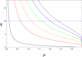
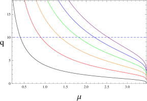
Figure 1: The charge $q$ as a function of the critical chemical potential $\mu$ for the operators ${\mathcal{O}}_{1}$ (left) and ${\mathcal{O}}_{2}$ (right). The curves from bottom to top correspond to the cases from the ground to fifth excited states. A typical blue dashed horizonal line with $q=10$ is shown to how to obtain the critical chemical potential of different excited states.

With the fixed charge $q$, there exists a critical value of the chemical potential $\mu$, below which the RN-AdS black hole solution is stable and the scalar field vanishes. Above this value, the charge static solution becomes unstable, the scalar condensate could form and lead to the spontaneously breaking of $U(1)$ gauge symmetry. Before solving the full dynamic equations of motion including Einstein equations numerically, we would adapt the same method as in [39], and find the critical value of $\mu$ with the fixed charge $q$. It is convenient to solve the time-independent scalar field equation at a RN-AdS black hole background with different values of chemical potential:

$$(\nabla_{\mu}\nabla^{\mu}-m^{2})\psi=q^{2}\,A_{\mu}A^{\mu}\,\psi\,,$$ (3.18)

with the mass $m^{2}=-2$. The above equation could be recognized as an eigenvalue problem with the eigenfunction $\psi$ and eigenvalue $q^{2}$. In a RN-AdS black hole with the fixed chemical potential background, we could obtain a series of eigenvalues of charge $q$. The smallest eigenvalue, that is, zero-mode of eigenvalue, corresponds to the ground state, while larger modes of eigenvalues correspond to excited states.

In Fig. 1, we show the charge $q$ as a function of the critical chemical potential $\mu$ for the operators ${\mathcal{O}}_{1}$ and ${\mathcal{O}}_{2}$ in the left and right panels, respectively. There are six curves on both plots denoting six different kinds of solutions from the ground to fifth excited states. In right panel, a typical blue dashed horizonal line with $q=10$ indicates the critical chemical potential $\mu_{c}=$ 0.41 (ground state), $0.90$ (1st-excited), $1.38$ (2nd-excited) and $1.82$ (3rd-excited), $2.20$ (4th-excited), $2.53$ (5th-excited) for the operator ${\mathcal{O}}_{2}$, respectively, which corresponds to the values of $q=10$ shown in Table 1. For each curve, the charge $q$ decreases with the increasing chemical potential $\mu$. We see that for the fixed amplitude $\mu$, the charge $q$ of excited state is larger than the ground state.

	$0$	$1$	$2$	$3$	$4$	$5$
$6$	0.67	1.46	2.15	2.67	3.04	3.26
$10$	0.41	0.90	1.38	1.82	2.20	2.53
$14$	0.29	0.65	1.00	1.34	1.66	1.96

Table 1: The critical chemical potential $\mu_{c}$ for the operator ${\mathcal{O}}_{2}$ from the ground to fifth excited states with the charges $q=6,10,14$, respectively.

In Table 1, we present the results of the critical chemical potential $\mu_{c}$ for the operator ${\mathcal{O}}_{2}$ from the ground to fifth excited states with the charges $q=6,10,14$, respectively. It is obvious that an excited state has a higher critical chemical potential than the ground state, which means the excited state has a higher critical charge density $\rho_{c}$. Due that the critical temperature is proportional to $\rho^{-1/2}_{c}$ in four-dimensional spacetime, the excited state has a lower critical temperature than the ground state , which is similar to the behavior in the probe limit [35].

3.1 Condensates

According to AdS/CFT duality, the expectation value of the condensate operator $\mathcal{O}_{i}$ could be connected to the scalar field $\psi^{(i)}$:

$$\langle{\mathcal{O}}_{i}\rangle=\sqrt{2}\psi^{(i)}\,,\quad i=1,2.$$ (3.19)

The values of condensates as functions of the temperature for the two operators ${\mathcal{O}}_{1}$ and ${\mathcal{O}}_{2}$ of excited states with the charge $q=6$ are shown in the left and right panels of Fig. 2, respectively. In both plots, the black, red and blue lines correspond to the ground state, first and second states, respectively. In the left panel, the condensate of the ground state for the operator $\mathcal{O}_{1}$ starts to curve upwards as ones approach low temperatures and appears similar to that of the probe limit. However, the condensate of excited states appears to converge as $T\rightarrow 0$, and there exists the constant condensate near zero temperature. Moreover, in contrast to the behavior of condensate for the operator $\mathcal{O}_{1}$ in probe limit [35], we find the condensate of the first-excited state is also smaller than that of the ground state in the left panel, however, it is interesting that the second-excited and higher excited states have larger condensate than the first excited state, which is different from the probe limit case. To clarify this issue, we plot an extra orange curve corresponding to the third excited state. In the right panel, the condensate of the excited states for the operator $\mathcal{O}_{2}$ appears to converge as the temperature $T\rightarrow 0$, and the condensate of each excited state is larger than the ground state, which appears similar to that of the probe limit.

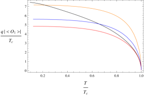
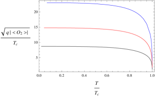
Figure 2: The values of condensates as functions of the temperature for the two operators ${\mathcal{O}}_{1}$ (left) and ${\mathcal{O}}_{2}$ (right) of excited states with the fixed charge $q=6$. In both plots, the black, red and blue lines denote the ground state, first and second states, respectively. In the left panel, the orange line denotes third excited state.

3.2 Conductivity

In this subsection we study the optical conductivity of the excited states of holographic superconductors with backreaction. According to the holographic duality, we can calculate electromagnetic fluctuations in the bulk geometry. Considering a time dependence perturbation of $\delta A=A_{x}(r)e^{-i\omega t}dx$, the linearized equation of the Maxwell equation is given as

$$A_{x}^{\prime\prime}+\left[\frac{g^{\prime}}{g}-\frac{\chi^{\prime}}{2}\right]A_{x}^{\prime}+\left[\left(\frac{\omega^{2}}{g^{2}}-\frac{\phi^{\prime 2}}{g}\right)e^{\chi}-\frac{2{q}^{2}\psi_{n}^{2}}{g}\right]A_{x}=0\,.$$ (3.20)

When implementing ingoing wave boundary conditions at the horizon, we could obtain the asymptotic behaviour of the gauge field $A_{x}$ at the boundary:

$$A_{x}=A_{x}^{(0)}+\frac{A_{x}^{(1)}}{r}+\cdots.$$ (3.21)

With the AdS/CFT correspondence and Ohm’s law, the conductivity can be computed by the following formula

$$\sigma(\omega)=-\frac{iA_{x}^{(1)}}{\omega A_{x}^{(0)}}\,.$$ (3.22)

In Eq. (3.20), the scalar field $\psi_{0}$ corresponds to the ground state, and the conductivity of the ground state has been studied in [6].

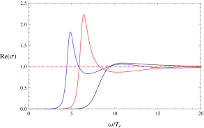
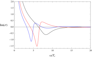
Figure 3: The real and imaginary parts of optical conductivity as functions of the frequency at the temperature $T/T_{c}\simeq 0.2$. In both plots, the black, red and blue lines denote the ground state, first and second states, respectively.

In Fig. 3, we present the AC conductivity as a function of the frequency $\omega$ at the low temperature $T/T_{c}\simeq 0.2$ for the operator ${\mathcal{O}}_{2}$ from the ground state to second excited state. The real and imaginary parts of conductivity are plotted in the left and right panels, respectively. In both plots, the black, red and blue lines correspond to the ground state, first and second states, respectively. From the imaginary part in the right panel, we could see the optical conductivity of excited states also develops a gap at certain frequency which can be identified as the minimum of the imaginary part of the optical conductivity [40]. Moreover, the gaps of excited states are located inside the gap of the ground state. It is interesting to note that there exists an additional peak in the imaginary part of the conductivity for the first excited state, and two additional peaks in $\text{Im}[\sigma]$ of the second excited state. Similar behaviours also appear in the real part of the conductivity. In the left panel of Fig. 3, there also exist additional peaks in the excited states. Moreover, the number of peaks corresponding to $n$-th excited state is equal to $n$. Recent work in [35] shows that in the probe limite case, there exists an additional pole in $\text{Im}[\sigma]$ and a delta function in $\text{Re}[\sigma]$ arising at low temperature inside the gap. In contrast to the probe limit case, we find that due to the introduction of backreaction, the pole and delta function can be broaden into the peaks with finite width.

4 Discussion

In this paper, we numerically solved the full dynamic equations of motion including Einstein equations, and constructed the holographic model of excited states of holographic superconductors with backreaction. When the temperature drops below the critical temperature, the condensate of holographic superconductor begins to appear, which could be regarded as the ground state solution. Further decreasing the temperature to another critical temperature, a new branch of solution with a node in radial direction begins to develop, which is the first excited state solution. As the temperature continues to decrease to lower values, we could obtain a series of excited states of holographic superconductor with corresponding critical temperatures, which is similar to the probe limit case. We also studied the optical conductivity in the excited states of holographic superconductors with backreaction. In contrast to the conductivity of the excited states in the probe limit case, it is very interesting to note that due to the introduction of backreaction, the pole and delta function in optical conductivity at the probe limit case can be transformed into the peaks with finite values at the backreaction case. Moreover, the number of peaks corresponding to $n$-th excited state is equal to $n$.

There are some interesting extensions of our work which we plan to investigate in future projects. First, in order to break the translational symmetry which means the momentum of charge carriers could be dissipated, the authors in [39] introduced a gravitational background lattice to the holographic model. It would be very interesting to study the optical conductivity of the excited states of holographic superconductor with holographic lattices. The second extension of our study is to explore the properties of holographic superconductors with backreaction using the semi-analytical techniques [41]. Finally, we are planning to investigate the excited states of the p-wave holographic superconductor with backreaction and study the excited vector condensates and optical conductivity in future work.

Acknowledgements

We would like to thank Jie Yang and Li Zhao for helpful discussion. Parts of computations were performed on the shared memory system at institute of computational physics and complex systems in Lanzhou university. This work was supported by the National Natural Science Foundation of China (Grants No. 11875151, No. 11522541 and No. 11704166).

References

- [1] J. M. Maldacena, “The Large N limit of superconformal field theories and supergravity,” Int. J. Theor. Phys. 38, 1113 (1999) [Adv. Theor. Math. Phys. 2, 231 (1998)] doi:10.1023/A:1026654312961, 10.4310/ATMP.1998.v2.n2.a1 [hep-th/9711200].
- [2] E. Witten, “Anti-de Sitter space and holography,” Adv. Theor. Math. Phys. 2, 253 (1998) doi:10.4310/ATMP.1998.v2.n2.a2 [hep-th/9802150].
- [3] O. Aharony, S. S. Gubser, J. M. Maldacena, H. Ooguri and Y. Oz, “Large N field theories, string theory and gravity,” Phys. Rept. 323, 183 (2000) doi:10.1016/S0370-1573(99)00083-6 [hep-th/9905111].
- [4] S. S. Gubser, “Breaking an Abelian gauge symmetry near a black hole horizon,” Phys. Rev. D 78, 065034 (2008) [arXiv:0801.2977 [hep-th]].
- [5] S. A. Hartnoll, C. P. Herzog and G. T. Horowitz, “Building a holographic superconductor,” Phys. Rev. Lett. 101, 031601 (2008) [arXiv:0803.3295 [hep-th]].
- [6] S. A. Hartnoll, C. P. Herzog and G. T. Horowitz, “Holographic superconductors,” JHEP 0812, 015 (2008) [arXiv:0810.1563 [hep-th]].
- [7] J. W. Chen, Y. J. Kao, D. Maity, W. Y. Wen and C. P. Yeh, “Towards A Holographic Model of D-Wave Superconductors,” Phys. Rev. D 81, 106008 (2010) [arXiv:1003.2991 [hep-th]].
- [8] F. Benini, C. P. Herzog, R. Rahman and A. Yarom, “Gauge gravity duality for d-wave superconductors: prospects and challenges,” JHEP 1011, 137 (2010) [arXiv:1007.1981 [hep-th]].
- [9] K. -Y. Kim and M. Taylor, “Holographic d-wave superconductors,” JHEP 1308, 112 (2013) [arXiv:1304.6729 [hep-th]].
- [10] S. S. Gubser and S. S. Pufu, “The Gravity dual of a p-wave superconductor,” JHEP 0811, 033 (2008) [arXiv:0805.2960 [hep-th]].
- [11] F. Aprile, D. Rodriguez-Gomez and J. G. Russo, “p-wave Holographic Superconductors and five-dimensional gauged Supergravity,” JHEP 1101, 056 (2011) doi:10.1007/JHEP01(2011)056 [arXiv:1011.2172 [hep-th]].
- [12] R. G. Cai, S. He, L. Li and L. F. Li, “A Holographic Study on Vector Condensate Induced by a Magnetic Field,” JHEP 1312, 036 (2013) doi:10.1007/JHEP12(2013)036 [arXiv:1309.2098 [hep-th]].
- [13] R. G. Cai, L. Li and L. F. Li, “A Holographic P-wave Superconductor Model,” JHEP 1401, 032 (2014) doi:10.1007/JHEP01(2014)032 [arXiv:1309.4877 [hep-th]].
- [14] B. D. Josephson, “Possible new effects in superconductive tunnelling,” Phys. Lett. 1, 251 (1962).
- [15] G. T. Horowitz, J. E. Santos and B. Way, “A holographic Josephson junction,” Phys. Rev. Lett. 106, 221601 (2011) [arXiv:1101.3326 [hep-th]].
- [16] Y. Q. Wang, Y. X. Liu and Z. H. Zhao, “Holographic Josephson junction in 3+1 dimensions,” [arXiv:1104.4303 [hep-th]].
- [17] M. Siani, “On inhomogeneous holographic superconductors,” [arXiv:1104.4463 [hep-th]].
- [18] E. Kiritsis and V. Niarchos, “Josephson junctions and AdS/CFT networks,” JHEP 1107, 112 (2011) [Erratum-ibid. 1110, 095 (2011)] [arXiv:1105.6100 [hep-th]].
- [19] Y. Q. Wang, Y. X. Liu and Z. H. Zhao, “Holographic p-wave Josephson junction,” [arXiv:1109.4426 [hep-th]].
- [20] Y. Q. Wang, Y. X. Liu, R. G. Cai, S. Takeuchi and H. Q. Zhang, “Holographic SIS Josephson junction,” JHEP 1209, 058 (2012) [arXiv:1205.4406 [hep-th]].
- [21] R. G. Cai, Y. Q. Wang and H. Q. Zhang, “A holographic model of SQUID,” JHEP 1401, 039 (2014) [arXiv:1308.5088 [hep-th]].
- [22] S. Takeuchi, “Holographic Superconducting Quantum Interference Device,” Int. J. Mod. Phys. A 30, no. 09, 1550040 (2015) [arXiv:1309.5641 [hep-th]].
- [23] H. F. Li, L. Li, Y. Q. Wang and H. Q. Zhang, “Non-relativistic Josephson Junction from Holography,” JHEP 1412, 099 (2014) [arXiv:1410.5578 [hep-th]].
- [24] S. Liu and Y. Q. Wang, “Holographic model of hybrid and coexisting s-wave and p-wave Josephson junction,” Eur. Phys. J. C 75, no. 10, 493 (2015) doi:10.1140/epjc/s10052-015-3692-2 [arXiv:1504.06918 [hep-th]].
- [25] Y. P. Hu, H. F. Li, H. B. Zeng and H. Q. Zhang, “Holographic Josephson Junction from Massive Gravity,” Phys. Rev. D 93, no. 10, 104009 (2016) doi:10.1103/PhysRevD.93.104009 [arXiv:1512.07035 [hep-th]].
- [26] Y. Q. Wang and S. Liu, “Holographic s-wave and p-wave Josephson junction with backreaction,” JHEP 1611, 127 (2016) doi:10.1007/JHEP11(2016)127 [arXiv:1608.06364 [hep-th]].
- [27] B. Kiczek, M. Rogatko and K. I. Wysokinski, “DC SQUID as a sensitive detector of dark matter,” arXiv:1904.00653 [hep-th].
- [28] S. S. Gubser, C. P. Herzog, S. S. Pufu and T. Tesileanu, “Superconductors from Superstrings,” Phys. Rev. Lett. 103, 141601 (2009) doi:10.1103/PhysRevLett.103.141601 [arXiv:0907.3510 [hep-th]].
- [29] J. P. Gauntlett, J. Sonner and T. Wiseman, “Holographic superconductivity in M-Theory,” Phys. Rev. Lett. 103, 151601 (2009) doi:10.1103/PhysRevLett.103.151601 [arXiv:0907.3796 [hep-th]].
- [30] J. P. Gauntlett, J. Sonner and T. Wiseman, “Quantum Criticality and Holographic Superconductors in M-theory,” JHEP 1002, 060 (2010) doi:10.1007/JHEP02(2010)060 [arXiv:0912.0512 [hep-th]].
- [31] S. A. Hartnoll, “Lectures on holographic methods for condensed matter physics,” Class. Quant. Grav. 26, 224002 (2009) [arXiv:0903.3246 [hep-th]].
- [32] C. P. Herzog, “Lectures on holographic superfluidity and superconductivity,” J. Phys. A 42, 343001 (2009) [arXiv:0904.1975 [hep-th]].
- [33] G. T. Horowitz, “Introduction to holographic superconductors,” Lect. Notes Phys. 828, 313 (2011) [arXiv:1002.1722 [hep-th]].
- [34] R. G. Cai, L. Li, L. F. Li and R. Q. Yang, “Introduction to Holographic Superconductor Models,” Sci. China Phys. Mech. Astron. 58, no. 6, 060401 (2015) [arXiv:1502.00437 [hep-th]].
- [35] Y. Q. Wang, T. T. Hu, Y. X. Liu, J. Yang and L. Zhao, “Excited states of holographic superconductors,” arXiv:1910.07734 [hep-th].
- [36] G. T. Horowitz and M. M. Roberts, “Holographic Superconductors with Various Condensates,” Phys. Rev. D 78, 126008 (2008) doi:10.1103/PhysRevD.78.126008 [arXiv:0810.1077 [hep-th]].
- [37] I. Amado, D. Arean, A. Jimenez-Alba, K. Landsteiner, L. Melgar and I. S. Landea, “Holographic Type II Goldstone bosons,” JHEP 1307, 108 (2013) doi:10.1007/JHEP07(2013)108 [arXiv:1302.5641 [hep-th]].
- [38] P. Breitenlohner and D. Z. Freedman, “Positive energy in anti-De Sitter backgrounds and gauged extended supergravity,” Phys. Lett. B 115, 197 (1982).
- [39] G. T. Horowitz and J. E. Santos, “General Relativity and the Cuprates,” JHEP 1306, 087 (2013) doi:10.1007/JHEP06(2013)087 [arXiv:1302.6586 [hep-th]].
- [40] G. T. Horowitz and M. M. Roberts, “Holographic Superconductors with Various Condensates,” Phys. Rev. D 78, 126008 (2008) doi:10.1103/PhysRevD.78.126008 [arXiv:0810.1077 [hep-th]].
- [41] G. Siopsis and J. Therrien, “Analytic Calculation of Properties of Holographic Superconductors,” JHEP 1005, 013 (2010) doi:10.1007/JHEP05(2010)013 [arXiv:1003.4275 [hep-th]].