Real-Time Reinforcement Learning

Abstract

Markov Decision Processes (MDPs), the mathematical framework underlying most algorithms in Reinforcement Learning (RL), are often used in a way that wrongfully assumes that the state of an agent’s environment does not change during action selection. As RL systems based on MDPs begin to find application in real-world, safety-critical situations, this mismatch between the assumptions underlying classical MDPs and the reality of real-time computation may lead to undesirable outcomes. In this paper, we introduce a new framework, in which states and actions evolve simultaneously and show how it is related to the classical MDP formulation. We analyze existing algorithms under the new real-time formulation and show why they are suboptimal when used in real time. We then use those insights to create a new algorithm Real-Time Actor-Critic (RTAC) that outperforms the existing state-of-the-art continuous control algorithm Soft Actor-Critic both in real-time and non-real-time settings. Code and videos can be found at github.com/rmst/rtrl.

Reinforcement Learning, has led to great successes in games (tesauro1994td; mnih2015human; silver2017mastering) and is starting to be applied successfully to real-world robotic control (schulman2015trust; hwangbo2019learning).

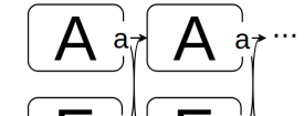
Figure 1: Turn-based interaction

Figure 2: Real-time interaction

The theoretical underpinning for most methods in Reinforcement Learning is the Markov Decision Process (MDP) framework (bellman1957markovian). While it is well suited to describe turn-based decision problems such as board games, this framework is ill suited for real-time applications in which the environment’s state continues to evolve while the agent selects an action (travnik). Nevertheless, this framework has been used for real-time problems using what are essentially tricks, e.g. pausing a simulated environment during action selection or ensuring that the time required for action selection is negligible (hwangbo2017control).

Instead of relying on such tricks, we propose an augmented decision-making framework - Real-Time Reinforcement Learning (RTRL) - in which the agent is allowed exactly one timestep to select an action. RTRL is conceptually simple and opens up new algorithmic possibilities because of its special structure.

We leverage RTRL to create Real-Time Actor-Critic (RTAC), a new actor-critic algorithm, better suited for real-time interaction, that is based on Soft Actor-Critic (haarnoja2018soft). We then show experimentally that RTAC outperforms SAC in both real-time and non-real-time settings.

1 Background

In Reinforcement Learning the world is split up into agent and environment. The agent is represented by a policy – a state-conditioned action distribution, while the environment is represented by a Markov Decision Process (Def. 1). Traditionally, the agent-environment interaction has been governed by the MDP framework. Here, however, we strictly use MDPs to represent the environment. The agent-environment interaction is instead described by different types of Markov Reward Processes (MRP), with the $T\!B\!M\!R\!P$ (Def. 2) behaving like the traditional interaction scheme.

Definition 1.

A Markov Decision Process (MDP) is characterized by a tuple with

(1) state space $S$,    (2) action space $A$,    (3) initial state distribution $\mu:S\to\mathbb{R}$,
(4) transition distribution $p:S\times S\times A\to\mathbb{R}$,    (5) reward function $r:S\times A\to\mathbb{R}$.

An agent-environment system can be condensed into a Markov Reward Process $(S,\mu,\kappa,\bar{r})$ consisting of a Markov process $(S,\mu,\kappa)$ and a state-reward function $\bar{r}$. The Markov process induces a sequence of states $(s_{t})_{t\in\mathbb{N}}$ and, together with $\bar{r}$, a sequence of rewards $(r_{t})_{t\in\mathbb{N}}=(\bar{r}(s_{t}))_{t\in\mathbb{N}}$.

As usual, the objective is to find a policy that maximizes the expected sum of rewards. In practice, rewards can be discounted and augmented to guarantee convergence, reduce variance and encourage exploration. However, when evaluating the performance of an agent, we will always use the undiscounted sum of rewards.

1.1 Turn-Based Reinforcement Learning

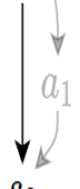
Figure 3: $T\!B\!M\!R\!P$

Usually considered part of the standard Reinforcement Learning framework is the turn-based scheme in which agent and environment interact. We call this interaction scheme Turn-Based Markov Reward Process.

Definition 2.

A Turn-Based Markov Reward Process $(S,\mu,\kappa,\bar{r})=T\!B\!M\!R\!P(E,\pi)$ combines a Markov Decision Process $E=(S,A,\mu,p,r)$ with a policy $\pi$, such that

$$\kappa(s_{t+1}|s_{t})=\int_{A}p(s_{t+1}|s_{t},a)\pi(a|s_{t})\ da\quad\text{and}\quad\bar{r}(s_{t})=\int_{A}r(s_{t},a)\pi(a|s_{t})\ da.\$$ (1)

We say the interaction is turn-based, because the environment pauses while the agent selects an action and the agent pauses until it receives a new observation from the environment. This is illustrated in Figure 2. An action selected in a certain state is paired up again with that same state to induce the next. The state does not change during the action selection process.

2 Real-Time Reinforcement Learning

Figure 4: $R\!T\!M\!R\!P$

In contrast to the conventional, turn-based interaction scheme, we propose an alternative, real-time interaction framework in which states and actions evolve simultaneously. Here, agent and environment step in unison to produce new state-action pairs $\boldsymbol{{x}}_{t+1}=({\hbox{\pagecolor{gray!17}$\displaystyle\ s_{t+1},a_{t+1}\ $}})$ from old state-action pairs $\boldsymbol{{x}}_{t}=({\hbox{\pagecolor{gray!17}$\displaystyle\ s_{t},a_{t}\ $}})$ as illustrated in Figures 2 and 4.

Definition 3.

A Real-Time Markov Reward Process $(\boldsymbol{{X}},\boldsymbol{{\mu}},\boldsymbol{{\kappa}},\bar{\boldsymbol{{r}}})=R\!T\!M\!R\!P(E,\boldsymbol{{\pi}})$ combines a Markov Decision Process $E=(S,A,\mu,p,r)$ with a policy $\pi$, such that

$$\boldsymbol{{\kappa}}({\hbox{\pagecolor{gray!17}$\displaystyle\ s_{t+1},a_{t+1}\ $}}|{\hbox{\pagecolor{gray!17}$\displaystyle\ s_{t},a_{t}\ $}})=p(s_{t+1}|s_{t},a_{t})\ \boldsymbol{{\pi}}(a_{t+1}|s_{t},a_{t})\quad\text{and}\quad\bar{\boldsymbol{{r}}}({\hbox{\pagecolor{gray!17}$\displaystyle\ s_{t},a_{t}\ $}})=r(s_{t},a_{t}).$$ (2)

The system state space is $\boldsymbol{{X}}=S\times A$. The initial action $a_{0}$ can be set to some fixed value, i.e. $\boldsymbol{{\mu}}({\hbox{\pagecolor{gray!17}$\displaystyle\ s_{0},a_{0}\ $}})=\mu(s_{0})\ \delta(a_{0}-c)$.

Note that we introduced a new policy $\boldsymbol{{\pi}}$ that takes state-action pairs instead of just states. That is because the system state $\boldsymbol{{x}}={\hbox{\pagecolor{gray!17}$\displaystyle\ (s,a)\ $}}$ is now a state-action pair and $s$ alone is not a sufficient statistic of the future of the stochastic process anymore.

2.1 The real-time framework is made for back-to-back action selection

In the real-time framework, the agent has exactly one timestep to select an action. If an agent takes longer that its policy would have to be broken up into stages that take less than one timestep to evaluate. On the other hand, if an agent takes less than one timestep to select an action, the real-time framework will delay applying the action until the next observation is made. The optimal case is when an agent, immediately upon finishing selecting an action, observes the next state and starts computing the next action. This continuous, back-to-back action selection is ideal in that it allows the agent to update its actions the quickest and no delay is introduced through the real-time framework.

To achieve back-to-back action selection, it might be necessary to match timestep size to the policy evaluation time. With current algorithms, reducing timestep size might lead to worse performance. Recently, however, progress has been made towards timestep agnostic methods (tallec2019making). We believe back-to-back action selection is an achievable goal and we demonstrate here that the real-time framework is effective even if we are not able to tune timestep size (Section LABEL:SectionExperiments).

2.2 Real-time interaction can be expressed within the turn-based framework

It is possible to express real-time interaction within the standard, turn-based framework, which allows us to reconnect the real-time framework to the vast body of work in RL. Specifically, we are trying to find an augmented environment $R\!T\!M\!D\!P(E)$ that behaves the same with turn-based interaction as would $E$ with real-time interaction.

In the real-time framework the agent communicates its action to the environment via the state. However, in the traditional, turn-based framework, only the environment can directly influence the state. We therefore need to deterministically "pass through" the action to the next state by augmenting the transition function. The $R\!T\!M\!D\!P$ has two types of actions, (1) the actions $\boldsymbol{{a}}_{t}$ emitted by the policy and (2) the action component $a_{t}$ of the state $\boldsymbol{{x}}_{t}=({\hbox{\pagecolor{gray!17}$\displaystyle\ s_{t},a_{t}\ $}})$, where $a_{t}=\boldsymbol{{a}}_{t-1}$ with probability one.

Definition 4.

A Real-Time Markov Decision Process $(\boldsymbol{{X}},A,\boldsymbol{{\mu}},\boldsymbol{{p}},\boldsymbol{{r}})=R\!T\!M\!D\!P(E)$ augments another Markov Decision Process $E=(S,A,\mu,p,r)$, such that

(1) state space $\boldsymbol{{X}}=S\times A$,   (2) action space is $A$,
(3) initial state distribution $\boldsymbol{{\mu}}(\boldsymbol{{x}}_{0})=\boldsymbol{{\mu}}({\hbox{\pagecolor{gray!17}$\displaystyle\ s_{0},a_{0}\ $}})=\mu(s_{0})\ \delta(a_{0}-c)$,
(4) transition distribution $\boldsymbol{{p}}(\boldsymbol{{x}}_{t+1}|\boldsymbol{{x}}_{t},\boldsymbol{{a}}_{t})=\boldsymbol{{p}}({\hbox{\pagecolor{gray!17}$\displaystyle\ s_{t+1},a_{t+1}\ $}}|{\hbox{\pagecolor{gray!17}$\displaystyle\ s_{t},a_{t}\ $}},\boldsymbol{{a}}_{t})=p(s_{t+1}|s_{t},a_{t})\ \delta(a_{t+1}-\boldsymbol{{a}}_{t})$
(5) reward function $\boldsymbol{{r}}(\boldsymbol{{x}}_{t},{\color[rgb]{.5,.5,.5}\boldsymbol{{a}}_{t}})=\boldsymbol{{r}}({\hbox{\pagecolor{gray!17}$\displaystyle\ s_{t},a_{t}\ $}},{\color[rgb]{.5,.5,.5}\boldsymbol{{a}}_{t}})=r(s_{t},a_{t})$.

(tap to see code)

Theorem 1.

​​ A policy $\boldsymbol{{\pi}}:A\times\boldsymbol{{X}}\to\mathbb{R}$ interacting with $R\!T\!M\!D\!P(E)$ in the conventional, turn-based manner gives rise to the same Markov Reward Process as $\boldsymbol{{\pi}}$ interacting with $E$ in real-time, i.e.

$$R\!T\!M\!R\!P(E,\boldsymbol{{\pi}})=T\!B\!M\!R\!P(R\!T\!M\!D\!P(E),\boldsymbol{{\pi}}).$$ (3)

Interestingly, the RTMDP is equivalent to a 1-step constant delay MDP (Walsh2008LearningAP). However, we believe the different intuitions behind both of them warrant the different names: The constant delay MDP is trying to model external action and observation delays whereas the RTMDP is modelling the time it takes to select an action. The connection makes sense, though: In a framework where the action selection is assumed to be instantaneous, we can apply a delay to account for the fact that the action selection was not instantaneous after all.

2.3 Turn-based interaction can be expressed within the real-time framework

It is also possible to define an augmentation $T\!B\!M\!D\!P(E)$ that allows us to express turn-based environments (e.g. Chess, Go) within the real-time framework (Def. LABEL:def:TBMDP in the Appendix). By assigning separate timesteps to agent and environment, we can allow the agent to act while the environment pauses. More specifically, we add a binary variable $b$ to the state to keep track of whether it is the environment’s or the agent’s turn. While $b$ inverts at every timestep, the underlying environment only advances every other timestep.

Theorem 2.

A policy $\boldsymbol{{\pi}}(\boldsymbol{{a}}|{s,b,a})=\pi(\boldsymbol{{a}}|s)$ interacting with $T\!B\!M\!D\!P(E)$ in real time, gives rise to a Markov Reward Process that contains (Def. LABEL:def:MRP-contains) the MRP resulting from $\pi$ interacting with $E$ in the conventional, turn-based manner, i.e.

$$T\!B\!M\!R\!P(E,\pi)\propto R\!T\!M\!R\!P(T\!B\!M\!D\!P(E),\boldsymbol{{\pi}})$$ (4)

As a result, not only can we use conventional algorithms in the real-time framework but we can use algorithms built on the real-time framework for all turn-based problems.

3 Reinforcement Learning in Real-Time Markov Decision Processes

Having established the RTMDP as a compatibility layer between conventional RL and RTRL, we can now look how existing theory changes when moving from an environment $E$ to $R\!T\!M\!D\!P(E)$.

Since most RL methods assume that the environment’s dynamics are completely unknown, they will not be able to make use of the fact that we precisely know part of the dynamics of RTMDP. Specifically they will have to learn from data, the effects of the "feed-through" mechanism which could lead to much slower learning and worse performance when applied to an environment $R\!T\!M\!D\!P(E)$ instead of $E$. This could especially hurt the performance of off-policy algorithms which have been among the most successful RL methods to date (mnih2015human; haarnoja2018soft). Most off-policy methods make use of the action-value function.

Definition 5.

The action value function $q_{E}^{\pi}$ for an environment $E=(S,A,\mu,p,r)$ and a policy $\pi$ can be recursively defined as

$$q_{E}^{\pi}(s_{t},a_{t})=r(s_{t},a_{t})+\mathbb{E}_{s_{t+1}\sim p(\cdot|s_{t},a_{t})}[\mathbb{E}_{a_{t+1}\sim\pi(\cdot|s_{t+1})}[q_{E}^{\pi}(s_{t+1},a_{t+1})]]$$ (5)

When this identity is used to train an action-value estimator, the transition $s_{t},a_{t},s_{t+1}$ can be sampled from a replay memory containing off-policy experience while the next action $a_{t+1}$ is sampled from the policy $\pi$.

Lemma 1.

In a Real-Time Markov Decision Process for the action-value function we have

$$q_{\text{{RTMDP(E)}}}^{\boldsymbol{{\pi}}}({\hbox{\pagecolor{gray!17}$\displaystyle\ s_{t},a_{t}\ $}},\boldsymbol{{a}}_{t})=r(s_{t},a_{t})+\mathbb{E}_{s_{t+1}\sim p(\cdot|s_{t},a_{t})}[\mathbb{E}_{\boldsymbol{{a}}_{t+1}\sim\boldsymbol{{\pi}}(\cdot|{\hbox{\pagecolor{gray!17}$\displaystyle\ s_{t+1},\boldsymbol{{a}}_{t}\ $}})}[q_{\text{{RTMDP(E)}}}^{\boldsymbol{{\pi}}}({\hbox{\pagecolor{gray!17}$\displaystyle\ s_{t+1},\boldsymbol{{a}}_{t}\ $}},\boldsymbol{{a}}_{t+1})]]$$ (6)

Note that the action $\boldsymbol{{a}}_{t}$ does not affect the reward nor the next state. The only thing that $\boldsymbol{{a}}_{t}$ does affect is $a_{t+1}$ which, in turn, only in the next timestep will affect $r(s_{t+1},a_{t+1})$ and $s_{t+2}$. To learn the effect of an action on $E$ (specifically the future rewards), we now have to perform two updates where previously we only had to perform one. We will investigate experimentally the effect of this on the off-policy Soft Actor-Critic algorithm (haarnoja2018soft) in Section LABEL:SacStruggles.

3.1 Learning the state-value function off-policy

The state-value function can usually not be used in the same way as the action-value function for off-policy learning.

Definition 6.

The state-value function $v_{E}^{\pi}$ for an environment $E=(S,A,\mu,p,r)$ and a policy $\pi$ is

$$v_{E}^{\pi}(s_{t})=\mathbb{E}_{a_{t}\sim\pi(\cdot|s_{t})}[r(s_{t},a_{t})+\mathbb{E}_{s_{t+1}\sim p(\cdot|s_{t},a_{t})}[v_{E}^{\pi}(s_{t+1})]]$$ (7)

The definition shows that the expectation over the action is taken before the expectation over the next state. When using this identity to train a state-value estimator, we cannot simply change the action distribution to allow for off-policy learning since we have no way of resampling the next state.

Lemma 2.

In a Real-Time Markov Decision Process for the state-value function we have

$$v_{\text{{RTMDP(E)}}}^{\boldsymbol{{\pi}}}({\hbox{\pagecolor{gray!17}$\displaystyle\ s_{t},a_{t}\ $}})=r(s_{t},a_{t})+\mathbb{E}_{s_{t+1}\sim p(\cdot|s_{t},a_{t})}[\mathbb{E}_{\boldsymbol{{a}}_{t}\sim\boldsymbol{{\pi}}(\cdot|{\hbox{\pagecolor{gray!17}$\displaystyle\ s_{t},a_{t}\ $}})}[v_{\text{{RTMDP(E)}}}^{\boldsymbol{{\pi}}}({\hbox{\pagecolor{gray!17}$\displaystyle\ s_{t+1},\boldsymbol{{a}}_{t}\ $}})]].$$ (8)

Here, $s_{t},a_{t},s_{t+1}$ is always a valid transition no matter what action $\boldsymbol{{a}}_{t}$ is selected. Therefore, when using the real-time framework, we can use the value function for off-policy learning. Since Equation 8 is the same as Equation 5 (except for the policy inputs), we can use the state-value function where previously the action-value function was used without having to learn the dynamics of the $R\!T\!M\!D\!P$ from data since they have already been applied to Equation 8.

3.2 Partial simulation

The off-policy learning procedure described in the previous section can be applied more generally. Whenever parts of the agent-environment system are known and (temporarily) independent of the remaining system, they can be used to generate synthetic experience. More precisely, transitions