Spectral modeling of type II supernovae

There are now hundreds of publicly available supernova spectral time series. Radiative transfer modeling of this data gives insights into the physical properties of these explosions such as the composition, the density structure, or the intrinsic luminosity—this is invaluable for understanding the supernova progenitors, the explosion mechanism, or for constraining the supernova distance.

However, a detailed parameter study of the available data has been out of reach due to the high dimensionality of the problem coupled with the still significant computational expense. We tackle this issue through the use of machine-learning emulators, which are algorithms for high-dimensional interpolation. These use a pre-calculated training dataset to mimic the output of a complex code but with run times orders of magnitude shorter. We present the application of such an emulator to synthetic type II supernova spectra generated with the tardis radiative transfer code. The results show that with a relatively small training set of 780 spectra we can generate emulated spectra with interpolation uncertainties of less than one percent. We demonstrate the utility of this method by automatic spectral fitting of two well-known type IIP supernovae; as an exemplary application, we determine the supernova distances from the spectral fits using the tailored-expanding-photosphere method. We compare our results to previous studies and find good agreement. This suggests that emulation of tardis spectra can likely be used to perform automatic and detailed analysis of many transient classes putting the analysis of large data repositories within reach.

1 Introduction

In recent years, improvements in instrumentation as well as the supply of targets have led to a tremendous increase in the volume of spectral data gathered for astrophysical transients of all kinds. At the same time, public databases such as the WISeREP archive (Yaron & Gal-Yam 2012) or the Open Supernova Catalog (Guillochon et al. 2017) have made access to this data easier than ever before; WISeREP alone provides 35484 spectra for 10809 transients.

In contrast, our tools for analyzing these large spectral datasets have lagged behind. We can distinguish between two sets of approaches for dealing with such numbers of spectra. The first, most prevalent, approach is to break the spectra down to a few easily-measurable diagnostic properties (e.g., line absorption velocities, equivalent widths), which are then studied for correlations (e.g., Gutiérrez et al. 2017, among many). The second approach is to use the spectra as input for machine learning techniques; exemplary applications include spectroscopic classification (e.g., Yip et al. 2004) or the detection of sub-classes, for example, of type Ia supernovae (Sasdelli et al. 2016). These approaches provide information about the specific measured quantities but do not provide a whole picture of the transient. Radiative transfer models have the power to infer underlying physical properties such as the composition and structure of the ejecta; we constrain these quantities by adjusting parametrized models of the emitting objects such that the simulated and observed spectra match. This provides, for example, information about the progenitor systems of the explosion for many kinds of transients (e.g., Hachinger et al. 2012 for SN Ic, Barna et al. 2017 for SN Iax). The main obstacle is the high cost of radiative transfer simulations; depending on the complexity of the underlying code, the time needed to calculate a single synthetic spectrum ranges between minutes and days. This is exacerbated by high-dimensional parameter spaces; we usually aim to determine a combination of various abundances, the density profile, photospheric temperatures and velocities (e.g., Dessart & Hillier 2006, Baron et al. 2007). It is prohibitively expensive to explore this parameter space automatically with radiative transfer models, as needed to identify the parameters that best reproduce the observed spectrum; instead, the current standard method is to optimize the agreement by hand, relying heavily on the expertise of the modeler (e.g., Stehle et al. 2005, Magee et al. 2017). This turns each spectroscopic analysis into an extremely time-consuming process that can only be done for very few objects. For example, only for three type IIP supernova has a full spectral time series been modeled in non-LTE in the last 15 years: SN 1999em (Baron et al. 2004, Dessart & Hillier 2006), SN 2005cs (Baron et al. 2007, Dessart et al. 2008) and SN 2006bp (Dessart et al. 2008).

One way to overcome the large computational expense of radiative transfer models in spectral fitting is to devise a fast algorithm that mimics the code. A very simple implementation of such an algorithm is interpolation in a pre-computed Cartesian grid. High-dimensional problems, such as supernovae, however, require the use of more complex algorithms known as emulators. In essence, the emulator learns the mapping from the simulation input to the output from a set of examples; the simulator, in this context, is treated as a black box. Emulators are used extensively, for example in engineering, but have, as of yet, not found widespread application in astrophysics. Some of the sparse use cases have been, the prediction of the nonlinear matter power spectrum (Heitmann et al. 2009), stellar spectra (Czekala et al. 2014), and type Ia supernova spectra (Lietzau 2017).

In this paper, we apply emulation to perform automated quantitative spectroscopic analysis of type II supernovae. We use Gaussian-process interpolation in the PCA space to reproduce the output of our radiative transfer code, a modified version of the Monte Carlo code Tardis (Vogl et al. 2019). With the emulator, we reduce the time for the calculation of a synthetic spectrum from hours to milliseconds; this, in turn, makes it possible to fit spectra using conventional optimization methods or to explore the parameter space with a sampler.

We showcase the emulator by inferring distances to type IIP supernovae using the tailored-expanding-photosphere method (tailored EPM; Dessart & Hillier 2006, Dessart et al. 2008). This method uses spectroscopic analysis of type IIP supernovae to obtain distances with small uncertainties, for example, for cosmological studies. A cosmological application requires a large number of uniformly studied supernovae, which will be made possible by the use of emulators. Such an endeavor will provide an independent, physics-based probe of the cosmic expansion history.

Sect. 2 provides a short introduction to supernova models and their use for parameter inference. Sect. 3 describes the library of synthetic spectra that forms the basis of our machine learning approach. Sect. 4 is dedicated to the presentation of the spectral emulator: the machine learning techniques, the training process, and the prediction step. In Sect. 5, we assess the predictive performance by comparing emulated and simulated spectra for a set of independent test models. We continue with the application of the emulator to the modeling of spectra of SN 1999em and SN 2005cs in Sect. 7. We show the application of measuring distances using the tailored EPM in Sect. 7.3. Sect. 8 summarizes the results and gives an outlook on the next steps.

2 Parametrized supernova models with Tardis

We use simple parametrized models of the supernova ejecta to make inferences about the supernova properties. In defining these models, we assume the ejecta to be spherically symmetric and in homologous expansion. This allows us to discretize the spectrum formation region into a set of shells that are specified by their composition, density, and expansion velocity. It is often useful to simplify the model specification further, for example, by assuming an analytic form for the density profile (e.g., a power law) or by assuming uniform abundances—this reduces the number of parameters considerably.

Since we do not simulate the creation of the radiation field self-consistently, we treat the radiation field at the inner boundary as a model parameter. Specifically, we assume a blackbody characterized by a temperature $T_{\mathrm{inner}}$; this is well motivated for type II supernovae (SNe II) since the continuum opacity from hydrogen leads to a full thermalization of the radiation field at high optical depths.

To assess if the thus defined parametrized model is consistent with the observations, we simulate the radiation transport through the discretized ejecta; then, we compare the synthetic and observed spectra. In Tardis (Kerzendorf & Sim 2014), we use a Monte Carlo approach based on the indivisible energy packet scheme of Lucy (1999a, b, 2002, 2003) to this end. The version used in this paper (Vogl et al. 2019) simulates the effects of bound-bound, bound-free, free-free, as well as collisional interactions on the radiation field; it accounts for NLTE effects in the excitation and ionization of hydrogen and calculates the thermal structure of the envelope from the balance of heating and cooling processes.

3 Creation of a SN II spectral training set

As a first step towards the spectral emulator, we need to calculate a set of synthetic SNe II spectra, which will serve as the training data. We have selected photospheric velocity $v_{\mathrm{ph}}$, photospheric temperature $T_{\mathrm{ph}}$, metallicity $Z$, time of explosion $t_{\mathrm{exp}}$ and steepness of the density profile $n=-\mathop{}\!\mathrm{d}{\ln{\rho}}/\mathop{}\!\mathrm{d}{\ln{r}}$ as the parameters of our model grid. The latter provides a simple parameterization of the density profile, which, as demonstrated, for example, by Chevalier (1976), Blinnikov et al. (2000) or Dessart & Hillier (2006), describes the outer density distribution with sufficient accuracy.

Most of the spectral evolution of photospheric phase SNe II, as well as the differences between individual objects, can be explained by variations in the expansion velocity, the temperature as well as the density profile. As such, the parameters usually considered in quantitative spectroscopic analyses, such as those of Dessart & Hillier (2006) or Dessart et al. (2008) are $v_{\mathrm{ph}}$, $T_{\mathrm{ph}}$ and $n$. In addition to these essential parameters, we include the metallicity $Z$. Observed SNe II show a wide range of metallicities (see e.g., Anderson et al. 2016, Taddia et al. 2016) and the associated changes to the spectrum are significant, in particular in the blue. For the purpose of inferring accurate distances, it is also important to allow for variations in the time of explosion $t_{\mathrm{exp}}$. While the effects on the shape of the spectral energy distribution (SED) are small, $t_{\mathrm{exp}}$ affects the absolute value of the flux through the modulation of the photospheric density (for any given density profile) and therefore the amount of continuum flux dilution (see e.g., Eastman et al. 1996). Other potentially relevant parameters are the abundances of CNO process elements, which have been investigated, for example, by Baron et al. (2007), as well as the H/He abundance ratio as studied, for example, by Dessart & Hillier (2006). For the first demonstration of our method, we refrain from varying these parameters and instead adopt CNO-cycle equilibrium values for the relevant abundances from Prantzos et al. (1986) as in Dessart & Hillier (2005, 2006).

Table 1 lists the ranges of parameters $v_{\mathrm{ph}}$, $T_{\mathrm{ph}}$, $Z$, $t_{\mathrm{exp}}$, and $n$ covered by our model grid. We have chosen the parameter space such that it allows for the modeling of a large variety of SNe II between roughly one and three weeks after explosion.

In practice, we cannot directly specify $T_{\mathrm{ph}}$ and $v_{\mathrm{ph}}$ since both are emergent and not input properties of the simulation; instead, we use the inner boundary temperature $T_{\mathrm{inner}}$, that is to say, the temperature of the injected blackbody radiation, and a simple analytic estimate for the photospheric velocity $v_{\mathrm{ph}}^{*}$. We set up a five-dimensional latin hypercube design (Stein 1987) in these parameters, which is optimized to fill the space nearly uniformly. In the next step, we perform radiative transfer calculations for the resulting set of 780 models and obtain synthetic spectra as well as the real values of $T_{\mathrm{ph}}$ and $v_{\mathrm{ph}}$. Fig. 1 shows pairwise projections for the completed set of parameters $v_{\mathrm{ph}}$, $T_{\mathrm{ph}}$, $Z$, $t_{\mathrm{exp}}$, and $n$. The grid of models displays a slight distortion in the $v_{\mathrm{ph}}$-$T_{\mathrm{ph}}$ plane as a result of our use of $v_{\mathrm{ph}}^{*}$ and $T_{\mathrm{inner}}$ as proxies for these quantities.

A common approach in machine learning is to generate a test set in addition to the training set to assess the predictive accuracy. We compute 225 models (in addition to the 780 training models). The parameters for these models are sampled uniformly from the same range of $v_{\mathrm{ph}}^{*}$, $T_{\mathrm{inner}}$, $Z$, $t_{\mathrm{exp}}$, and $n$ as covered by the training data. We include the properties of the test data in Fig. 1 to facilitate the comparison between the sets of models.

One of the challenges in the setup of the model grid is deciding how large the training set of models really needs to be. Ideally, the number of training models should be large enough to guarantee that the interpolation uncertainty in the spectra is not the dominant contribution to the error in the inferred parameters; at the same time, the training size should be kept as small as possible for reasons of computational expediency. In practice, the best possible trade-off is difficult to identify since the conversion from the interpolation errors in the spectra to errors in the parameters is nontrivial. To be on the safe side, however, one can aim to have the interpolation uncertainty significantly smaller than the systematic mismatch between model and observation; for the parameter space we consider, this is indeed the case for the training set we have used (see Sect. 5).

Table 1: Parameter range covered by the spectral library.

	$v_{\mathrm{ph}}$ [km/s]	$T_{\mathrm{ph}}\,$[K]	$Z\,[Z_{\odot}]$	$t_{\mathrm{exp}}\,$[days]	n
min	3700	6300	0.1	6.5	6
max	10500	10000	3.0	22.0	16

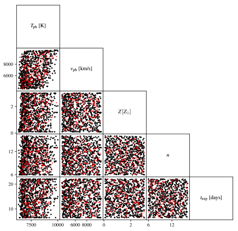
Figure 1: Scatterplot matrix of the parameters of the training data (black) and test data (red) of the spectral emulator.

4 Spectral emulator

We use the synthetic spectra from the previous section to create two separate emulators: one for spectra and one for absolute magnitudes. We set up these emulators in two steps. First, we preprocess the training data and synthesize absolute magnitudes; this is followed by dimensionality reduction of the preprocessed spectra through PCA decomposition. Second, we train Gaussian processes to interpolate the spectra within the PCA space and to predict absolute magnitudes.

4.1 Preprocessing and dimensionality reduction

The synthetic spectra have a range of values that varies widely both with wavelength and between models. In addition, they contain non-negligible Monte Carlo noise. For the successful application of machine learning techniques, it is crucial to preprocess the noisy, unscaled data to standardize it and to remove unwanted sources of variations. We start by smoothing the spectra with a fifth-order Savitzky-Golay filter (Savitzky & Golay 1964) to reduce the effect of Monte Carlo noise. Savitzky-Golay filtering performs well in preserving the shape of spectral features, even weak ones, which makes it a popular choice for denoising astrophysical spectra (see e.g., Hügelmeyer et al. 2007, Poznanski et al. 2010, Sasdelli et al. 2014). Next, we approximately correct for the variations in the position of spectral features between models by Doppler shifting each spectrum by the photospheric velocity $v_{\mathrm{ph}}$. This roughly maps the absorption minimum of a spectral feature to the same wavelength for all models. Since we do not assume a distance for fitting an observed spectrum (see Sect. 7), we can standardize the spectral library further by discarding the information about the luminosity. Specifically, we normalize the shifted synthetic spectra to have unit flux at $6000\text{\,}\AA$; this provides a good standardization of the continuum flux levels between models since no strong line features form at this position. Finally, we apply a linear transformation to the fluxes in each wavelength bin such that in each bin the values for the full spectral library span a range from -0.5 to 0.5 (see appendix A). For each preprocessing step, we restrict the considered wavelength range to the minimum range needed to model the observations in Sect. 7. In practice, this corresponds to a wavelength window from roughly $3200\text{\,}\AA 9500\text{\,}\AA$. In contrast, we only smooth the test spectra but do not preprocess them further: we will compare them to the emulated spectra in the same fashion one would do for observational data.

In the final step, we reduce the dimensionality of our spectral library. Each preprocessed spectrum consists of a few thousand wavelength bins, a number which by far exceeds that of the physical parameters used in its creation. To obtain a less correlated, more compact representation of our data, we use Principal Component Analysis (PCA). PCA has been applied successfully to observed spectra of a wide range of astrophysical objects, including QSOs (e.g., Francis et al. 1992), stars (e.g., Bailer-Jones et al. 1998), galaxies (e.g., Connolly et al. 1995) and supernovae (e.g., Sasdelli et al. 2014, Williamson et al. 2019). The basic idea is to find an orthogonal basis for the data that is a linear transformation of the original but where the axes are aligned with the directions of maximal variance. Since by construction each successive principal component explains less of the variance in the data, we can reduce the dimensionality of our dataset by truncating the basis; instead of using the full set of $N_{\mathrm{L}}$ principal component eigenvectors, where $N_{\mathrm{L}}$ is the number of spectra in the spectral library, we use only the first $N<N_{\mathrm{L}}$ components. We select the dimensionality $N$ of the truncated basis through cross-validation on the training sample since our main goal is the accurate prediction of synthetic spectra. The cross-validation performance increases, at first, as more principal components are included but at some point levels off when the additional components stop to contain meaningful information; it is at this point that we truncate the PCA basis. For the spectral emulator presented in this paper, this approach leads us to use $N=80$ principal components, which explain 99.97% of the total variance; this is a significant reduction compared to the original $\approx 1500$ wavelength bins. If necessary, the number of principal components can be reduced even further with only minor losses in accuracy. By projecting each preprocessed spectrum $\hat{f}_{k}$ onto the basis vectors $\xi_{i}$ of the thus truncated basis, we obtain a compact representation of the input data in terms of a set of $N$ principal component weights $\{w_{ik}\}$. From these principal component weights, we can lossily reconstruct every input spectrum as a linear combination of the principal components $\xi_{i}$ and the mean spectrum $\xi_{\mu}=\sum_{k}^{N_{L}}\hat{f}_{k}/N_{\mathrm{L}}$:

$$\hat{f}_{k}\approx\xi_{\mu}+\sum_{i=1}^{N}w_{ik}\xi_{i}$$ (1)

For the selected number of principal components, the mean fractional reconstruction error for this procedure is 0.26 %.

In addition to the spectral preprocessing and the dimensionality reduction, we synthesize Johnson-Cousins B,V, I magnitudes from the unprocessed synthetic spectra. These serve as training data for a separate emulator that predicts absolute photometric magnitudes for a set of model parameters $v_{\mathrm{ph}}$, $T_{\mathrm{ph}}$, $Z$, $t_{\mathrm{exp}}$, and $n$. This allows us, in Sect. 7, to convert the inferred parameters from the spectral fitting into a distance estimate based on the observed photometry.

4.2 Gaussian process interpolation

Spectra

To predict a spectrum for a new set of input parameters $\theta=(v_{\mathrm{ph}},T_{\mathrm{ph}},Z,n,t_{\mathrm{exp}})$, we have to interpolate between the principal component weights $\{w_{ik}\}$, which form the compressed version of our spectral library. We choose to model the weights $w_{i}$ for each principal component $\xi_{i}$ independently since, by construction, the weights for the different components are at least linearly uncorrelated. As in Czekala et al. (2014), we use Gaussian processes (e.g., Rasmussen 2006) for the interpolation. Gaussian processes (GPs) are a powerful, probabilistic tool for regression analysis, which are steadily gaining in popularity in the astrophysical community (see, e.g., Rajpaul et al. 2015, Foreman-Mackey et al. 2017). As a non-parametric method, GPs offer increased flexibility for modeling complicated signals compared to more conventional approaches such as linear or polynomial regression.

Fundamentally speaking, GPs provide a generalization of the Gaussian probability distribution from finite-dimensional random variables to functions. Following this analogy, each GP is characterized by a mean- and a covariance function. The covariance function $k$ controls the covariance between the distribution of random function values at any two points $\theta,\theta^{{}^{\prime}}$ in the parameter space. As such, it determines the properties of the functions that can be drawn from the GP including, for example, their smoothness, periodicity and so forth. In the context of regression analysis, the choice of the covariance function sets the prior distribution of functions that we expect to see in the data. A particularly important class of covariance functions are the so-called stationary covariance functions, which do not depend on the positions $\theta,\theta^{{}^{\prime}}$ in the input space but only on their distance $r=||\theta-\theta^{{}^{\prime}}||$. The most commonly used members of this class include the squared exponential, the Matérn and the rational quadratic covariance function (see, e.g., Rasmussen 2006, Murphy 2013). The type of covariance function is a hyperparamter of the machine-learning approach and can, similar to the preprocessing steps, be set based on the cross-validation performance. After some experimentation, we have adopted covariance functions from the Matérn family:

$$k_{\mathrm{Matern}}(r)=\sigma_{f}^{2}\frac{2^{1-\nu}}{\Gamma(\nu)}\left(\sqrt{2\nu}r\right)^{\nu}K_{\nu}\left(\sqrt{2\nu}r\right)$$ (2)

Here, $\sigma_{f}^{2}$ denotes the signal variance, $\nu$ is a parameter that regulates the smoothness of the GP, $\Gamma$ is the gamma function, and $K_{\nu}$ is the modified Bessel function of the second kind. Since we do not expect the weights, which encode our MC synthetic spectra, to be noise free, we include an additive contribution of homoscedastic white noise in the covariance function

$$k(r)=k_{\mathrm{Matern}}(r)+\sigma_{n}^{2}\,\delta(r).$$ (3)

Here, $\sigma_{n}^{2}$ is the noise variance and $\delta$ the Dirac delta function. We complete the description of the covariance function by defining the distance as

$$r^{2}(\theta,\theta^{{}^{\prime}})=(\theta-\theta^{{}^{\prime}})^{\mathrm{T}}M\,(\theta-\theta^{{}^{\prime}}),$$ (4)

where $M$ can be any positive semidefinite matrix. For reasons of simplicity, we only consider diagonal matrices of the following type

$$M=\begin{bmatrix}\frac{1}{{l_{v_{\mathrm{ph}}}}^{2}}{}&&&\\ &\frac{1}{{l_{T_{\mathrm{ph}}}}^{2}}&&\\ &&\ddots&\\ &&&\frac{1}{{l_{t_{\mathrm{exp}}}}^{2}}\end{bmatrix}$$ (5)

in this paper. For this choice of metric, each dimension of the input space $(v_{\mathrm{ph}},T_{\mathrm{ph}},Z,n,t_{\mathrm{exp}})$ has its own characteristic length-scale $(l_{v_{\mathrm{ph}}},\dots,l_{t_{\mathrm{exp}}})$ for variations in the function values.

Finally, to make predictions, we have to move from the prior distribution of functions to a posterior distribution of functions that agree with the training data. Mathematically speaking, this is achieved by conditioning the zero-mean prior GP on the observed values. The conditional GP has a non-zero mean function $w_{i}(\theta)$ that is determined by the values $w_{ik}$ of the training data and the covariances $k_{i}(\theta,\theta_{k})$ between the location $\theta$ and the training locations $\theta_{k}$. The relevant expressions for the predictive mean and variance can be found in standard textbooks such as Rasmussen (2006, their Algorithm 2.1). Given a set of hyperparameters $(\sigma_{n}^{2},\sigma_{f}^{2},l_{v_{\mathrm{ph}}},\dots,l_{t_{\mathrm{exp}}},\nu)$, these equations yield the interpolated values for the principal component weight as well as an estimate of the interpolation uncertainty. The parameter $\nu$ regulating the smoothness properties of the process is difficult to constrain through the data; after some experimentation, we have adopted $\nu=3/2$, corresponding to functions that are once mean-square differentiable. We set the rest of the hyperparameters by numerically maximizing the marginal likelihood of the training data under the GP model. We repeat this process $N$ times since we model the weights $w_{i}$ for each principal component $\xi_{i}$ independently.

Eq. 1 allows us to predict ‘preprocessed’ spectra $\hat{f}(\theta)$ using the trained GPs. To arrive at a spectrum that we can compare to observations, we have to reverse some of the preprocessing steps used to standardize the input spectra for PCA in Sect. 4.1. This involves inverting the linear transformation applied to map the fluxes in each bin to the range $[-0.5,0.5]$, as well as blue-shifting the spectrum by the photospheric velocity $v_{\mathrm{ph}}$.

Absolute magnitudes

In Sect. 4.1, we removed the luminosity information from the synthetic spectra to standardize them further for PCA. We train additional GPs for the prediction of the absolute magnitudes, which we need for our distance inferences in Sect. 7.

As part of the data preprocessing, we have synthesized Johnson-Cousins S={B,V,I} magnitudes $M_{S}$ from the unprocessed synthetic spectra. Before we use these as training data for the GPs, we remove the variation in the magnitudes introduced by differences in the physical sizes of the supernova models. Specifically, we transform from absolute magnitudes to magnitudes at the position of the photosphere

$$m_{S}^{\mathrm{ph}}=M_{S}+5\log\frac{R_{\mathrm{ph}}}{$10\text{\,}\mathrm{p}\mathrm{c}$},$$ (6)

where $R_{\mathrm{ph}}=v_{\mathrm{ph}}t_{\mathrm{exp}}$. We model each bandpass with a GP with a Matérn covariance function (see, Eq. 2) that has a smoothness parameter $\nu=5/2$. The hyperparameters $(\sigma_{n}^{2},\sigma_{f}^{2},l_{v_{\mathrm{ph}}},\dots,l_{t_{\mathrm{exp}}})$ for the individual bandpasses are set in the same fashion as for the spectral emulator. Finally, to predict absolute magnitudes for a new set of input parameters $\theta=(v_{\mathrm{ph}},T_{\mathrm{ph}},Z,n,t_{\mathrm{exp}})$, we evaluate the trained GP and subtract $5\log(R_{\mathrm{ph}}/$10\text{\,}\mathrm{p}\mathrm{c}$)$.

5 Evaluation of the emulator performance

To allow the reliable inference of parameters from supernova spectra, it is crucial that the emulator reproduces the output of our simulation code tardis to high precision. We assess the predictive performance of our method by comparing the predicted spectra and absolute magnitudes to a set of independently collected test data. Our strategy for the calculation of the 225 test models is described in detail in Sect. 3 and the associated preprocessing procedure in Sect. 4.1.

Spectra

In Fig. 2, we compare simulated and emulated spectra for a subset of the test models; the selected subset approximately spans the range of deviations encountered in the full test data. We have scaled the emulated spectra back to physical units for the comparison of spectral shapes. Despite covering a wide variety of spectral appearances, including, for example, SEDs with very broad or very narrow features, with or without line blanketing, the agreement is overall excellent. In addition, in most cases, the deviations are within the 95% confidence interval of the emulator prediction with areas of larger residuals corresponding to regions with increased emulation uncertainties.

In order to quantify the test performance, we need to define a quality metric that expresses the mismatch between two spectra in a single number. We use the mean fractional error

$$\mathrm{MFE}=\frac{1}{N_{\lambda}}\sum_{i=1}^{N_{\lambda}}\frac{|f_{\lambda,i}^{\mathrm{emu}}-f_{\lambda,i}^{\mathrm{test}}|}{f_{\lambda,i}^{\mathrm{test}}},$$ (7)

where $f_{\lambda,i}^{\mathrm{test}}$ and $f_{\lambda,i}^{\mathrm{emu}}$ are the test and emulated spectra respectively, and $N_{\lambda}$ is the number of wavelength bins. By using the MFE instead of, for example, the mean squared error, we give approximately the same weight to the red (low flux) and blue (high flux) parts of the spectrum. We summarize the test performance in the top left panel of Fig. 2, which shows a histogram of the MFEs for the entire test sample. The median MFE is 0.64 %, confirming the excellent agreement found by visual inspection. For 95 percent of the test spectra the deviation is less than 1.2 %; for the remaining 5 percent maximum differences of around 2 % are possible. To assess how the emulator performance varies within the parameter space, we have modified the scatterplot matrix of the test parameters to include the color-coded MFE (see Fig. 3). The figure demonstrates that a significant fraction of the cases with appreciable mismatches can be traced back to models near the edge of the training parameter space (or even outside of it). We also notice a slight decrease in performance towards lower velocities, temperatures, and higher metallicities. This trend is to be expected since the complexity of the SED increases in these directions of the parameter space. For example, in the case of velocity, we move from a few blended features to a forest of individual metal lines; each of these lines evolves individually, in a nonlinear fashion making it difficult to model the spectral evolution based on a PCA decomposition.

Absolute magnitudes

For the purpose of measuring accurate distances, it is crucial that we can accurately predict the luminosity for any combination of input parameters. We assess the accuracy of our approach by comparing the synthetic photometry of the test models to the absolute magnitudes predicted by the emulator. As shown in Fig. 4, the median difference between the predicted and true magnitudes is less than 0.0012 mag; this confirms that the emulator provides an unbiased estimate of the true model luminosity. The accuracy of the predictions decreases from the redder to the bluer bandpasses but is nevertheless excellent in all cases; the slight decrease can be easily explained by the different amounts of line blanketing in each filter. In all filters, 68 % of the models show differences of less than 0.007 mag corresponding to errors in the model flux of less than 0.7 %. For 95 % of the models, the errors are less than 0.02 mag yielding maximum flux errors of around 1.8 %. Thus, in virtually all cases, the accuracy of the emulator is much higher than the uncertainties in most real photometric data. Finally, in Fig. 5, we demonstrate that, as in the case of spectra, the emulator provides sensible estimates for the predictive uncertainties.

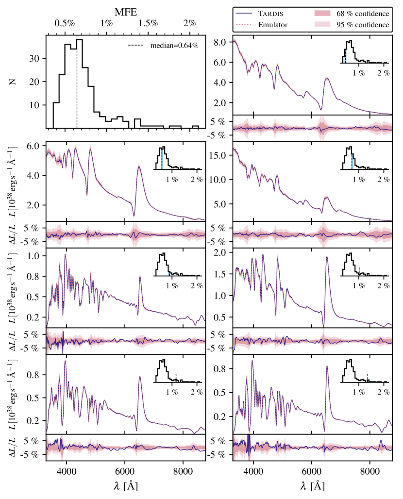
Figure 2: Evaluation of the emulator performance. The test performance is summarized in the top left panel, which shows a histogram of the test errors; specifically, the MFE (see Eq. 7) is displayed. The other panels provide a direct comparison between emulated and simulated spectra for a subset of the test data. Each panel contains a histogram of the test errors, in which the position of the current model is highlighted. To highlight the subtle differences between the predicted and true spectra, the fractional difference $\Delta L/L$ is shown in the lower section of each panel (solid blue line). In both sections, the shaded regions indicate the $68\%$ and $95\%$ confidence intervals for the prediction of the emulator.

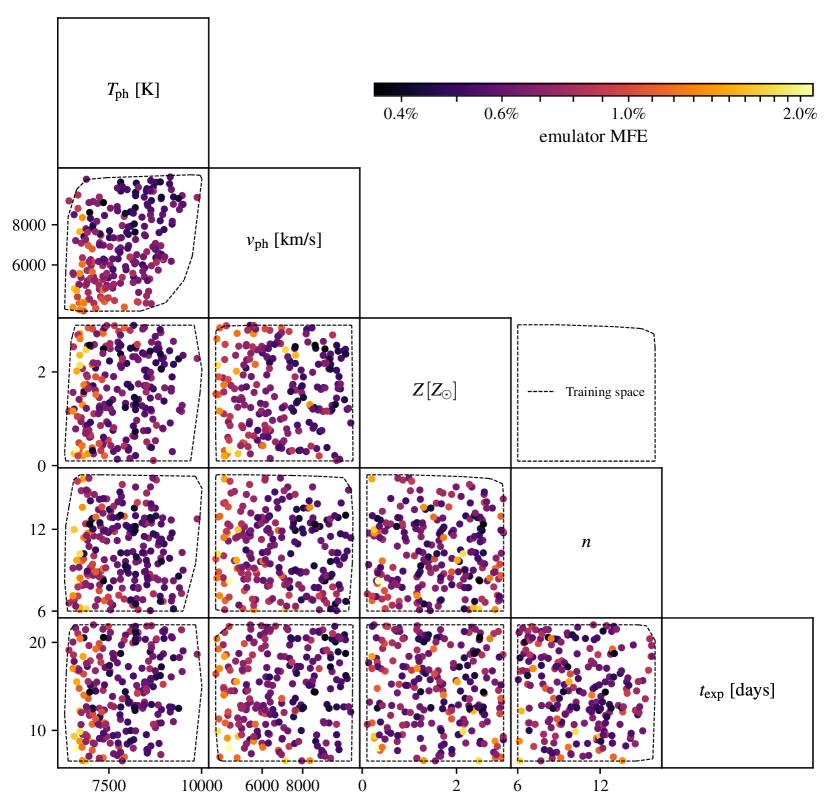
Figure 3: Test errors for the spectral emulator as a function of the input parameters. We show the color-coded MFE (see Eq. 7) between emulated and simulated spectra for all two dimensional projections of the test parameters. The region enclosed by the dashed black line indicates the parameter space covered by the training data.

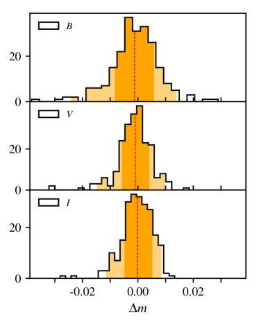
Figure 4: Differences $\Delta m$ between predicted and true magnitudes for the B, V and I bandpasses. The median of each distribution is marked with a dashed red line. We indicate the central 68% and 95% intervals in orange and light orange respectively.

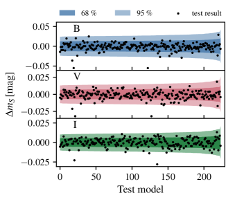
Figure 5: Comparison of the predicted uncertainties to the actual differences, $\Delta m$, between predicted and true magnitudes. For each bandpass (B, V and I), we show the 68% and 95% confidence interval for the predicted magnitudes as well as their actual deviations from the magnitudes of the test models (denoted ‘test result’).

6 Learning behavior of the emulator

In this section, we address questions about the number of models needed for a desired accuracy, the adequacy of the adopted methods, and how the emulator compares to the standard approach of picking the best-fitting model from the grid.

We start by creating a learning curve for the spectral emulator as shown in Fig. 6. The learning curve shows the accuracy of the emulator as a function of the number of models used for training, for both the test and the training sample. We keep the number of principal components fixed, thus starting with a minimum training size of 80. In the investigated regime, the mean error on the training set is almost constant at around 0.5 %. At least part of this error can plausibly be attributed to the MC noise inherent to the models. From the small training errors, we conclude that our model does not suffer from high bias, that is to say, the model is flexible enough to provide a satisfactory fit to the training data. The mean test error decreases steadily from its initial value of 1.7 % as the number of training instances is increased and quickly drops below 1 %. Finally, for the maximum training size, a test score of 0.7 % is reached. At this point, the difference between training and test score is small but non-negligible. The gap between the scores will be reduced even further as more training instances are added since the test score is still decreasing (albeit at a slower rate). We conclude that our model generalizes well and does not overfit the training data.

Finally, we compare the emulator to the often used approach of simply picking the best fitting model from the grid. In Fig. 7, we show the test scores for both approaches as a function of the number of training instances; the plot highlights the massive reduction in the number of models that are needed to achieve a given precision. The emulator with the minimum considered training size of 80 outperforms the method of picking the nearest model even when the full set of 780 spectra is used. To get a rough estimate of how many models would be needed to match the final accuracy of 0.7 % of the emulator, we linearly extrapolate the learning curve in log-linear space; this yields on the order of 15000 spectra. This is a conservative lower limit for the number of needed models since it generously assumes a constant learning rate.

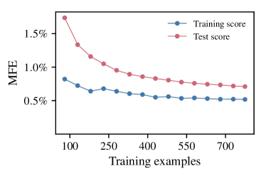
Figure 6: Learning curve for the spectral emulator. The error on the training sample as well as the test sample is shown as a function of the number of models used in the training. The quoted errors are the mean of the individual errors, which, in turn, are the MFE for each spectrum. For each training size, we select five different realizations at random and average the resulting errors.

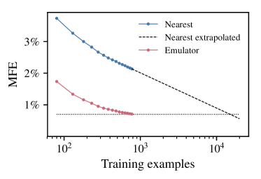
Figure 7: Learning behavior of the emulator as a function of the number of spectra used in the training in comparison to the more naive approach of picking the closest spectrum.

7 Modeling observations

With the spectral emulator, we can fit SN II spectral time series in an automated fashion. For a first demonstration, we select SN 1999em and SN 2005cs as our test objects. SN 1999em is considered by many to be the prototype of a type II supernova, whereas SN 2005cs is a more peculiar, subluminous object. Both are among the best-observed type II supernovae, with extensive datasets including photometry and spectroscopy at UV, optical and infrared wavelengths (Leonard et al. 2001, 2002, Hamuy et al. 2001, Dessart & Hillier 2006, Pastorello et al. 2006, 2009, Tsvetkov et al. 2006, Bufano et al. 2009). Both SNe have been studied with detailed NLTE radiative transfer models using Cmfgen (Dessart & Hillier 2006, Dessart et al. 2008) and Phoenix (Baron et al. 2004, 2007). We will compare the results of our automated fits to these analyses, which have been conducted carefully by hand. In our comparison, we focus on the studies of Dessart & Hillier (2006) and Dessart et al. (2008), which model more epochs and have published the relevant inferred parameters, namely $T_{\mathrm{ph}},v_{\mathrm{ph}}$ and $n$. In the final step, we infer distances to the supernovae from our fits using the tailored-expanding-photosphere method.

7.1 Likelihood for parameter inference

We use a standard multi-dimensional Gaussian likelihood function for parameter inference. In this case, the log-likelihood of an observed spectrum $f_{\lambda}^{\mathrm{obs}}$ with $N_{\mathrm{pix}}$ spectral bins is given by

$$\ln{p(f_{\lambda}^{\mathrm{obs}}|\theta_{\mathrm{SN}},E(B-V))}=-\frac{1}{2}\left(\mathrm{R}^{\mathrm{T}}\mathrm{C}^{-1}\mathrm{R}+\ln\det\mathrm{C}+N_{\mathrm{pix}}\ln 2\pi\right)$$ (8)

where

$$R=f_{\lambda}^{\mathrm{obs}}-f_{\lambda}(\theta_{\mathrm{SN}},E(B-V))$$ (9)

are the residuals with respect to the emulated, reddened spectrum $f_{\lambda}$ and $C$ is the pixel-by-pixel covariance matrix (e.g., Czekala et al. 2014). As before, $\theta_{\mathrm{SN}}=(v_{\mathrm{ph}},T_{\mathrm{ph}},Z,n,t_{\mathrm{exp}})$ are the parameters of our SN model and $E(B-V)$ is the color excess. The residuals have pixel-to-pixel correlations mostly due to imperfections in the model calculations (see Czekala et al. 2014). For example, a slight error in the ionization balance of a given element will lead to features in the synthetic spectrum that are either systematically too weak or too strong, producing highly correlated residuals in these regions. If these correlations are not accounted for in the covariance matrix $C$, the uncertainties of the inferred parameters will be severely underestimated (Czekala et al. 2014). We find typical uncertainties for the photospheric temperature of the order of a few Kelvin if we only include the interpolation uncertainty and the photon count noise; thus, without a good statistical model for the correlated residuals, the inferred uncertainties are essentially meaningless. For the purpose of a first demonstration, we resort to a simple maximum likelihood approach with homoscedastic white noise, that is to say, a diagonal, constant covariance matrix. Our rationale for using homoscedastic white noise instead of a combination of the heteroscedastic photon noise and the interpolation uncertainties is that the systematic mismatches between model and observation are the dominant error component in most regions; ignoring it means that we assign highly variable and essentially meaningless weights to different parts of the spectrum.

7.2 Fitting observed spectra

We want to compare our framework for parameter inference to the quantitative spectroscopic analyses of Dessart & Hillier (2006) and Dessart et al. (2008)—detailed NLTE studies conducted carefully by hand by experts. To allow an unbiased comparison of the inferred parameters, we copy key assumptions of their study. First, we adopt solar metallicities for the non-CNO processed elements. Second, we use the same elapsed times since explosion as utilized in the calculation of their spectral models; this is particularly important for the comparison of photospheric temperatures, which are sensitive to this parameter. Third, we adopt a color excess of $E(B-V)=0.1$ towards SN 1999em and a color excess of $E(B-V)=0.04$ towards SN 2005s in concordance with Dessart & Hillier (2006) and Dessart et al. (2008). We redden the emulated spectra by this color excess according to the Cardelli, Clayton, & Mathis (1989) law with $R_{V}=3.1$. Finally, we blueshift the observed spectra by the peculiar velocities of their host galaxies, which we assume to be $770\text{\,}\mathrm{km}\text{\,}{\mathrm{s}}^{-1}$ (Leonard et al. 2002, Dessart & Hillier 2006) for SN 1999em and $466\text{\,}\mathrm{km}\text{\,}{\mathrm{s}}^{-1}$ (Dessart et al. 2008) for SN 2005s. A log of the spectra used as well as relevant model parameters such as the time since explosion utilized in the calculation of the spectral models can be found in footnote 17.

Table 2: Log of modeled spectra for (a) SN 1999em, and (b) SN 2005cs.

JD (+$2\,451\,474.04$)	Date	Source	${t_{\mathrm{exp}}}$
17.9	9 Nov.	H01	9.67
22.9	14 Nov.	H01	11.21
27.9	19 Nov.	H01	22.00

(a) SN 1999em

JD (+$2\,453\,549$)	Date	Source	${t_{\mathrm{exp}}}$
12.25	9 Jul.	D08	14.67
13.5	10 Jul.	F14	16.12
14.5	11 Jul.	P06	15.33
17.0	14 Jul.	P06	16.11
19.4	16 Jul.	P200	19.40

(b) SN 2005cs

SN 1999em

We model three epochs of SN 1999em, covering a time span between roughly two to four weeks after explosion. In Fig. 8, we show the maximum likelihood emulated spectra in comparison to the observations, highlighting the good agreement between the two. For each spectral epoch, a table with the inferred maximum likelihood parameters as well as the literature values from Dessart & Hillier (2006) is attached to the plot. Despite using vastly different methods for calculating synthetic spectra and for adjusting them to match the observations, we find good agreement in the inferred parameters, with maximum differences of only $285\,$K in photospheric temperature, $351\,$km/s in photospheric velocity and $0.8$ in the steepness of the density profile. We visualize this in Fig. 11, which plots our values for $v_{\mathrm{ph}}$ and $T_{\mathrm{ph}}$ against those of Dessart & Hillier (2006). Whereas our best fit parameters for $T_{\mathrm{ph}}$ and $v_{\mathrm{ph}}$ fall below or above those of Dessart & Hillier (2006) depending on the epoch, we find systematically higher values for the power law density index $n$. To investigate this, we examine the influence of the steepness of the density profile on the emergent spectra in Fig. 9 using the epoch of the 9th of November as an example. From this, it becomes clear that in the discussed regime of values (density indexes between 10 and 11) the changes in the emergent spectra are small. We see that only strong lines such as H$\alpha$, which form over a wide range of velocities, are affected at all and even those only slightly.

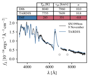
(a) November 9

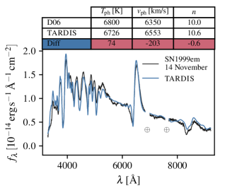
(b) November 14

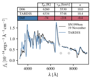
(c) November 19

Figure 8: Spectroscopic analysis of SN 1999em. The three subfigures show comparisons between observed (black) and best-fit emulated spectra (blue); the best-fit has been determined through a maximum likelihood approach as outlined in Sect. 7.2. Each spectral comparison is combined with a table of the inferred parameters, the literature values from Dessart & Hillier (2006) (D06) and the difference between the two. Since the observations have not been corrected for telluric absorption, we exclude the regions of strongest absorption from the fit (marked $\oplus$).

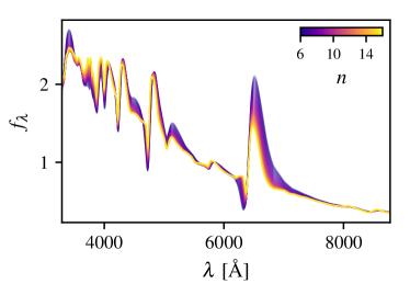
Figure 9: Variation of the spectral shape with the steepness of the density profile $n$. We plot specific flux $f_{\lambda}$ in arbitrary units for a sequence of emulated spectra where only the power law density index $n$ is modified between spectra; the remaining parameters have been chosen to provide a good fit to SN 1999em for the 9th of November (see Fig. 8 a). We color code the plotted spectra by the power law density index $n$.

SN 2005cs

We analyze five closely-spaced spectral observations of SN 2005cs, between roughly two to three weeks after explosion. For the first four epochs, there are spectral models from Dessart et al. (2008) at comparable epochs, allowing a comparison of the inferred parameters. The last epoch on the 16th of July is used only for our measurement of the distance to the supernova in Sect. 7.3. As for SN 1999em, we show the maximum likelihood emulated spectra combined with tables of the inferred and literature parameters in Fig. 10. Again, we find good agreement in the inferred parameters with only few exceptions.

For the photospheric velocity, the epoch of the 14th of July stands out, which shows a deviation of $569\,$km/s. In particular, the increase in velocity compared to the previous epoch is puzzling. It can be understood in the following way: as discussed in Dessart & Hillier (2006, §3.3.3), spectral fits yield differences on the $10\text{\,}\mathrm{\char 37\relax}$ level in the photospheric velocity depending on which set of lines the fit is optimized on. For the two epochs, our automated fits likely attribute varying weights to certain features, thus giving rise to the inconsistent velocity estimates; for example, on the 11th the Ca infrared triplet absorption is not fit well, forming at too low velocities, whereas on the 14th the absorption minimum is matched much better.

Regarding photospheric temperature, the earliest epoch has the largest deviation, which is $767\,$K. We do not know for certain what causes this significant difference. Nevertheless, it is striking that the epoch with the largest deviation in temperature also has the smallest wavelength coverage. We show a full comparison of measured temperatures and velocities in Fig. 11.

Similar to the case of SN 1999em, our maximum likelihood fits favor slightly steeper density profiles than those proposed by Dessart et al. (2008); instead of $n=10$, we find values between 10.9 and 12.4. As outlined in the previous section, these variations in the density profile only induce very moderate changes in the emergent spectrum and should not be overinterpreted. This applies, in particular, to the increase of the best-fit value for $n$ in the last two epochs; this is likely not due to a physical effect but an artifact of our current method of using different density profiles for each epoch and our maximum likelihood approach. This will be alleviated by fitting the entire spectral time series at the same time.

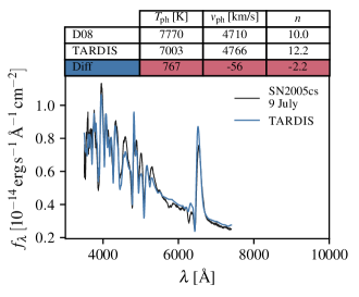
(a) July 9

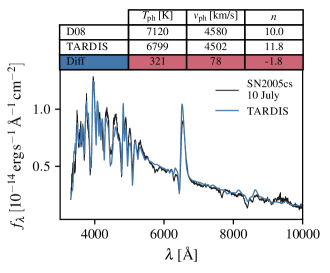
(b) 10 July

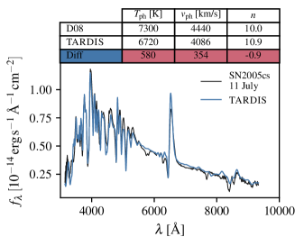
(c) 11 July

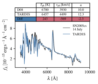
(d) July 14

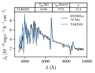
(e) July 16

Figure 10: Spectroscopic analysis of SN 2005cs. See Fig. 8 for a description of the layout. Here, values for the parameter comparison are taken from Dessart et al. (2008) (D08). In (e), we only show the inferred parameters since this epoch has not been modeled in Dessart et al. (2008).

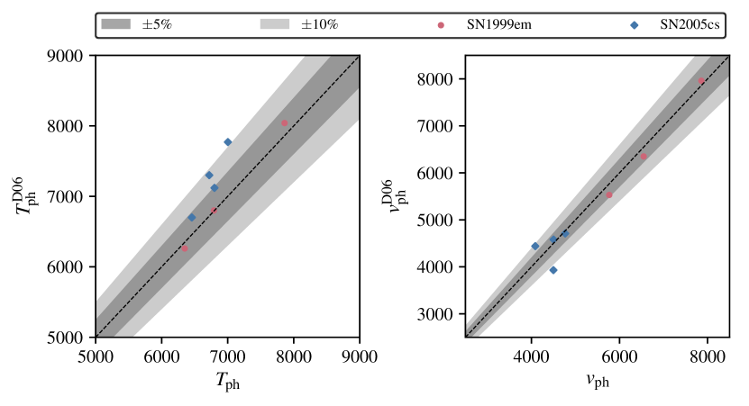
Figure 11: Comparison of the photospheric temperatures $T_{\mathrm{ph}}$ and velocities $v_{\mathrm{ph}}$ inferred from our automated spectral fits to those of Dessart & Hillier (2006) and Dessart et al. (2008): $T_{\mathrm{ph}}^{\mathrm{D06}}$ and $v_{\mathrm{ph}}^{\mathrm{D06}}$. The dashed black line indicates perfect agreement between the measurements, whereas the grey shaded regions denote deviations of 5 % and 10 % respectively.

7.3 Distance measurements

In the past, the need to optimize the fit quality by hand and eye combined with the high cost of radiative transfer calculations have made distance measurements from SN II spectral models (e.g., Baron et al. 2004, Dessart & Hillier 2006) a very labor-intensive process. Automated fits based on spectral emulation revise this picture completely.

We use a variant of the tailored EPM (Dessart & Hillier 2006, Dessart et al. 2008) to constrain the distance $D$ to the supernovae. As a first step, we measure the photospheric angular diameter $\Theta=R_{\mathrm{ph}}/D=v_{\mathrm{ph}}t_{\mathrm{exp}}/D$ for each epoch. We compare the apparent magnitudes $m_{S}$ of our best fit model

$$m_{S}=M_{S}(\theta^{*})-5\log(\Theta)+A_{S}$$ (10)

to the observed photometry ${m_{S}}^{\mathrm{obs}}$ for different values of $\Theta$. Here, $A_{S}$ is the broadband dust extinction for the bandpass S={B,V,I} and $M_{S}(\theta^{*})$ is the predicted absolute magnitude for the best fit parameters $\theta^{*}$. We adopt the photospheric angular diameter $\Theta^{*}$ that minimizes the squared difference between observed and model magnitudes:

$$\Theta^{*}=\underset{\Theta}{\operatorname{arg\,min}}\sum_{S}\left(m_{S}-{m_{S}}^{\mathrm{obs}}\right)^{2}$$ (11)

Our approach to tailored EPM is technically identical to Dessart & Hillier (2006) and Dessart et al. (2008) but avoids the detour of parametrizing the model magnitudes by a blackbody color temperature and a dilution factor.

Finally, we determine the time of explosion and the distance through a Bayesian linear fit to the time evolution of the ratio of the photospheric angular diameter $\Theta$ and the photospheric velocity $v_{\mathrm{ph}}$. To be more specific, we obtain the time of explosion from the intercept with the time axis and the distance from the inverse of the slope. In our analysis, we assume that the uncertainties are Gaussian and that they have standard deviations of 10 % of the measured values as in Dessart & Hillier (2006) and Dessart et al. (2008). We use a half-Cauchy prior for the slope of the regression curves, corresponding to a uniform distribution for the angle between the straight lines and the time axis. We adopt informative priors for the time of explosion, which we will discuss in the context of the individual supernovae below.

Our sources of photometry are Leonard et al. (2002) for SN 1999em (as listed in Table 1 of Dessart & Hillier 2006) and Pastorello et al. (2009) for SN 2005cs. If there is no coincident photometric observation for a given spectral epoch, we linearly interpolate the magnitudes from the nearest epochs. We list all magnitudes used in our tailored EPM analysis in footnote 21.

Table 3: Interpolated BVI photometry for the epochs of spectral observations.

JD (+$2\,451\,474.04$)	Date	B	V	I
17.9	9 Nov.	14.02	13.84	13.48
22.9	14 Nov.	14.25	13.81	13.44
27.9	19 Nov.	14.47	13.86	13.40

(a) SN 1999em

JD (+$2\,453\,549$)	Date	B	V	I
12.25	9 Jul.	14.75	14.59	14.30
13.5	10 Jul.	14.83	14.60	14.26
14.5	11 Jul.	14.92	14.58	14.25
17.0	14 Jul.	15.09	14.67	14.25
19.4	16 Jul.	15.26	14.70	14.28

(b) SN 2005cs

SN 1999em

For a first demonstration of the emulator, we adopt an informative Gaussian prior for the time of explosion based on the tailored EPM analysis of Dessart & Hillier (2006), which finds $t_{0}$ = JD 2 451 474.04$\pm 1.0$. While the time of explosion for SN 1999em is not well constrained through the photometry, many objects have limits that are as tight or tighter than the adopted prior for $t_{0}$; this applies, for example, to SN 2005cs as we will discuss in the next section.

With the prior for $t_{0}$ defined, we apply the tailored EPM as outlined above. We summarize the inputs as well as the results of our analysis in Fig. 13. In the figure, we combine a table of the ratios of photospheric angular diameter and velocity $\Theta/v_{\mathrm{ph}}$, a visualization of the Bayesian linear regression, and a corner plot of the inferred distance and time of explosion. We find a distance of ${11.4}^{+1.0}_{-0.9}\,$Mpc, which is in excellent agreement with the Cepheid distance to the host galaxy of ${11.7}\pm 1\,$Mpc (Leonard et al. 2003). It is important to keep in mind that the quoted uncertainties are solely statistical and depend both on the adopted prior for $t_{0}$ and the assumed uncertainties for $\Theta/v_{\mathrm{ph}}$. Finally, we point out that the regression is only weakly informative on the time of explosion, that is to say, the posterior distribution for $t_{0}$ is only modified slightly compared to the prior.

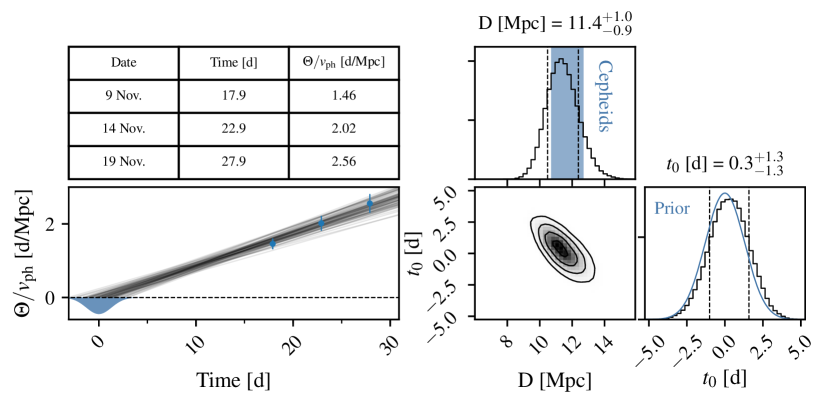
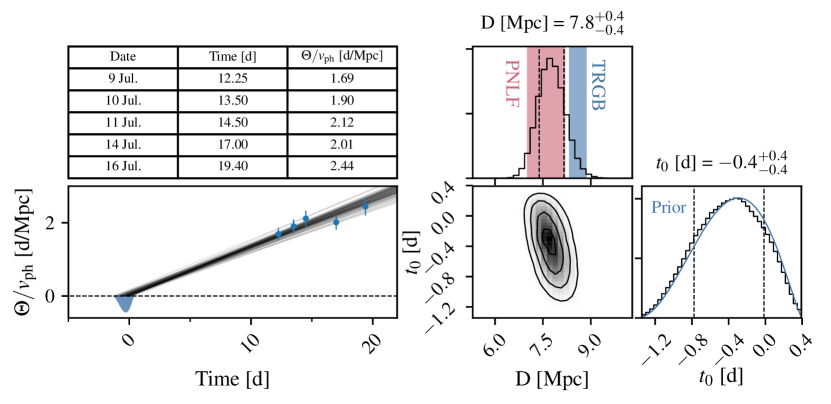
Figure 12: Tailored EPM for SN 1999em. The lower left panel shows the evolution of the ratio of the photospheric angular diameter $\Theta$ and the photospheric velocity $v_{\mathrm{ph}}$ with time (blue circles). Here, we measure the time with respect to JD $2\,451\,474.04$. We tabulate the plotted values in the upper left panel. Finally, we perform a Bayesian linear fit to this data. Our prior for the time of explosion is indicated by the blue shaded region. From the posterior distribution, we show 100 randomly sampled regression curves for illustrative purposes. The right half of the figure features a corner plot of the inferred parameters. Our distance measurement is in excellent agreement with the Cepheid distance of Leonard et al. (2003), which is indicated by the blue shaded region.

Figure 13: Tailored EPM for SN 2005cs. For a description of the figure layout see Fig. 13. The time zero point is at JD $2\,453\,549.0$. Within the statistical uncertainties, the inferred distance agrees with the measurement of Ciardullo et al. (2002) using the planetary nebula luminosity function (PNLF), as well as that of McQuinn et al. (2016) based on the tip of the red giant branch (TRGB).

SN 2005cs

As opposed to SN 1999em, the time of explosion for SN 2005cs is constrained tightly by photometric observations. Based on the non-detection at JD = $2\,453\,548.43$ and the detection at JD = $2\,453\,549.41$, Pastorello et al. (2009) identify JD = $2\,453\,549.0\pm 0.5$ as the time of shock breakout. In our prior for $t_{0}$, we make small changes to this result to incorporate two basic arguments. First, the prior probability that the first detection is coincident with the explosion should be zero. Secondly, the probability that the explosion occurred before the last non-detection should be non-negligible due to the limited depth of the image. Based on these considerations, we construct the Beta prior shown in Fig. 13. Our prior peaks shortly after the last non-detection and has a width that is compatible with the quoted uncertainties of Pastorello et al. (2009). We derive the distance to the supernova as illustrated in Fig. 13 and obtain a value of ${7.8}^{+0.4}_{-0.4}\,$Mpc.

In contrast to SN 1999em, the distance to SN 2005cs is not constrained through Cepheids. NED lists 50 individual distance measurements spanning a range of values between $2.45\,$Mpc and $12.2\,$Mpc with a median distance of $7.935\,$Mpc. Based on spectral modeling of SN 2005cs, Dessart et al. (2008) find a distance of $8.9\pm 0.5\,$Mpc using tailored EPM in the BVI bandpasses and Baron et al. (2007) ${7.9}^{+0.7}_{-0.6}\,$Mpc with the SEAM method. Independent state-of-the-art measurements come from Ciardullo et al. (2002), who derive a distance of $7.6\pm 0.6\,$Mpc using the planetary nebula luminosity function (PNLF), and McQuinn et al. (2016), who infer a value of $8.58\pm 0.10\,$Mpc from the tip-of-the-red-giant-branch method.

Overall, the agreement between our measurement and the results above is satisfactory given the uncertainties of the individual methods. The 15% deviation to the tailored EPM distance of Dessart et al. (2008), however, warrants investigation. We find that roughly half of the discrepancy arises from differences in the time of explosion. From the evolution of the ratio of photospheric angular diameter and velocity, Dessart et al. (2008) obtain an explosion epoch that is earlier than ours by about a day. They explain the difference between their estimate and those based on non-detections (specifically, Pastorello et al. 2006, in their paper) with a short time delay between the beginning of the expansion and the optical brightening. After adjusting the time of explosion, the remaining deviation is around 7 % and thus within the expected range.

8 Conclusions and outlook

In this paper, we demonstrate the use of spectral emulation to predict the SN II spectra and magnitudes generated by tardis (Kerzendorf & Sim 2014, Vogl et al. 2019).

The key ingredient of our approach is the creation of a low-dimensional space for the interpolation of synthetic spectra through the combination of appropriate data preprocessing and dimensionality reduction by PCA. In this space, we train Gaussian processes to predict preprocessed, dimensionality-reduced spectra for new sets of input parameters. In the final step, we reverse the preprocessing procedure to obtain a spectrum that can be compared to observations. This method emulates the output of our radiative transfer code to high precision; we demonstrate this by comparing emulated and simulated spectra for a large number of test models. On average, the emulator prediction deviates from the simulation by around 0.64 % (as measured by the MFE)—this is much smaller than both observational and model uncertainties. Not only are the interpolation uncertainties small but we can also estimate them sensibly through our use of Gaussian processes; this will allow us, in the future, to propagate these errors into the uncertainties of the inferred parameters.

We complement the spectral emulator with an emulator for absolute magnitudes; we have discarded the luminosity information in the spectral emulator to standardize the spectra and to obtain better predictive performance. The training data are Johnson-Cousins B,V, I magnitudes that have been synthesized from the unprocessed training spectra. We remove variations in the luminosity that result from differences in the physical sizes of the supernova models by transforming the magnitudes to the position of the photosphere; then, we interpolate the transformed magnitudes using Gaussian processes. This allows us to predict absolute magnitudes with an average precision of better than 0.01 mag, which is significantly smaller than typical observational uncertainties.

The emulator is not only accurate, but also orders of magnitude faster ($\approx 10\,$ms) than our simulator Tardis ($\approx 100000\,$s)—this makes it possible to fit spectra automatically. We demonstrate this by performing maximum likelihood parameter estimation for spectral time series of SN 1999em and SN 2005cs. The inferred parameters of the supernovae show good agreement with those of Dessart & Hillier (2006) and Dessart et al. (2008), who studied these objects using the Cmfgen code. Similarly, the distances that we infer from our fits are consistent with the best available measurements from the literature.

As a next step, we will develop a more detailed likelihood to infer accurate uncertainties for a complete parameter estimate. The emulator and an advanced likelihood will then allow the use of type IIP supernova for accurate cosmological distance determinations.

Appendix A Min-max normalization

Min-max normalization scales each feature (here, the fluxes in a bin) individually such that it spans the range [Min, Max] for the training data. The min-max normalized flux $f_{\lambda,ij}^{\mathrm{norm}}$ for spectrum $i$ in bin $j$ is given by

$$f_{\lambda,ij}^{\mathrm{norm}}=\frac{f_{\lambda,ij}-\underset{i}{\operatorname{min}}f_{\lambda,ij}}{\underset{i}{\operatorname{max}}f_{\lambda,ij}-\underset{i}{\operatorname{min}}f_{\lambda,ij}}\left(\mathrm{Max}-\mathrm{Min}\right)+\mathrm{Min}.$$ (12)

This linear transformation can be easily reversed in the prediction step of the emulator.