Black Hole Coagulation: Modeling Hierarchical Mergers in Black Hole Populations

Abstract

Data from the LIGO and Virgo detectors has confirmed that stellar-mass black holes can merge within a Hubble time, leaving behind massive remnant black holes. In some astrophysical environments such as globular clusters and AGN disks, it may be possible for these remnants to take part in further compact-object mergers, producing a population of hierarchically formed black holes. In this work, we present a parameterized framework for describing the population of binary black hole mergers, while self-consistently accounting for hierarchical mergers. The framework casts black holes as particles in a box which can collide based on an effective cross-section, but allows inputs from more detailed astrophysical simulations. Our approach is relevant to any population which is comprised of second or higher generation black holes, such as primordial black holes or dense cluster environments. We describe some possible inputs to this generic model and their effects on the black hole merger populations, and use the model to perform Bayesian inference on the catalog of black holes from LIGO and Virgo’s first two observing runs. We find that models with a high rate of hierarchical mergers are disfavored, consistent with previous population analyses. Future gravitational-wave events will further constrain the inputs to this generic hierarchical merger model, enabling a deeper look into the formation environments of binary black holes.

April 1, 2020

1 Introduction

The Advanced Laser Interferometer Gravitational Wave Observatory (LIGO)  (The LIGO Scientific Collaboration, 2015) and Virgo (Accadia & et al, 2012) detectors have and will continue to discover gravitational waves (GW) from coalescing binary black holes (BBHs) and neutron stars. So far, several tens of binary black hole detection candidates have been reported in O3, LIGO’s current observing run, and several hundreds more detections are expected over the next five years (The LIGO Scientific Collaboration and the Virgo Collaboration, 2016a, b). As the cosmic census these surveys provide grows more comprehensive, these observations will discriminate between formation scenarios of compact-object binaries. (Mandel & O’Shaughnessy, 2010; Rodriguez et al., 2016; Breivik et al., 2016; Nishizawa et al., 2016). A few formation scenarios invoke “hierarchical” growth of binary black holes in which some black holes are themselves products of previous mergers. These hierarchical mergers could occur in globular clusters (Portegies Zwart & McMillan, 2002; Gültekin et al., 2006), AGN disks (see,e.g. McKernan et al., 2012; Bartos et al., 2017; Yang et al., 2019; McKernan et al., 2019), or nuclear star clusters (Antonini & Rasio, 2016). Alternatively, the hierarchical merger components could have been produced in the early universe due to primordial density fluctuations forming primordial black holes (Clesse & García-Bellido, 2015, 2017; Belotsky et al., 2019). Notably, hierarchical growth produces distinctive signatures in the mass and spin distribution (Fishbach et al., 2017; Yang et al., 2019; Gerosa & Berti, 2017; McKernan et al., 2019; Kimball et al., 2019), the most generic of which is a population of spinning black holes. For some realizations of these models’ parameters, several groups have made predictions about the black hole mass and spin distribution (Rodriguez et al., 2016; McKernan et al., 2019; Belczynski et al., 2017). Additional investigations have assessed whether existing observations are compatible with these models, focusing on the individual event GW170729 (Chatziioannou et al., 2019; Yang et al., 2019; Kimball et al., 2019).

In this work, we introduce a generic, parameterized framework that accounts for binary black holes which form through hierarchical mergers. The method treats black holes as particles in a box which undergo collisions based on an effective cross section. This framework can incorporate a wide range of submodels and prescriptions, enabling one to create models that are purely phenomenological or instead heavily based on detailed astrophysical investigations and simulations. We provide a concrete implementation of our framework, including astrophysically realistic initial conditions. Using existing gravitational wave observations, we perform Bayesian inference on our parameterized model.

Our paper is organized as follows. In §2, we describe our framework for hierarchical mergers and some parameterizations within the framework, illustrating them with simple examples. We also describe our fiducial initial conditions for binary black hole populations. In §3, we show how to constrain this parameterized model through comparison with gravitational wave observations from LIGO and Virgo’s first and second observing runs. In §4, we discuss the results of our parameter inference on the LIGO-Virgo data, the overall efficacy of our framework, and possible extensions to the parameterizations explored herein. Finally, we summarize the results of our investigation in §5.

2 Parameterized hierarchical formation of binary black holes

2.1 General framework

We employ a flexible method for self-consistently generating mass and spin distributions for binary black holes which include a subpopulation of hierarchical mergers. Rather than model the complex dynamics of individual stellar environments, we build a parameterized phenomenological model which describes the aggregate properties of merging binaries in the local universe, using volume-averaged coupling coefficients. Our framework incorporates three generic physical processes. First, black holes coagulate when pairs of compact objects merge into single compact objects which may remain in the population. Second, we allow for depletion, where some compact objects leave dense environments and no longer have an opportunity to merge with other objects. Finally, we allow for augmentation, where some process introduces new compact objects to the hierarchical interacting environment (e.g., BHs from stellar collapse or AGN disk dynamics).

Following similar investigations (Christian et al., 2018; Lissauer, 1993), we model these effects with a Monte Carlo procedure, designed to approximate a continuous-time coagulation equation (Smoluchowski, 1916), which has the qualitative form

$$\partial_{t}f(x;t) =\frac{1}{2}\int dx^{\prime}dx^{\prime\prime}f(x^{\prime};t)f(x^{\prime\prime};t)\Gamma(x^{\prime},x^{\prime\prime};t)\delta(x_{\mathrm{rem}}(x^{\prime\prime},x^{\prime})-x)-\int dx^{\prime}f(x;t)f(x^{\prime};t)\Gamma(x,x^{\prime};t)$$ (1)

$$+r(x;t)-d(x;t)$$

where here $x$ denotes black hole parameters, $f(x;t)$ denotes the BH parameter distribution function at time $t$, $\Gamma(x,x^{\prime};t)$ denotes a volume-averaged interaction rate (i.e. coagulation), and $r(x;t)$ and $d(x;t)$ are the augmentation and depletion rates of black holes with parameters $x$ at time $t$. The first integral describes the accumulation of black holes with parameters $x$ due to mergers of pairs of black holes with parameters $x^{\prime},x^{\prime\prime}$. The delta function enforces that the final parameters $x$ are produced by a merger of BHs with parameters $x^{\prime},x^{\prime\prime}$. The function $x_{\rm rem}(x,x^{\prime})$ computes the remnant parameters from merger component parameters $x$ and $x^{\prime}$ . The second integral accounts for the decrease of black holes with parameters $x$ due to mergers with other black holes with parameters $x^{\prime}$, and its integrand $f(x;t)f(x^{\prime};t)\Gamma(x,x^{\prime};t)$ is equivalent to the merger rate as a function of parameters. In the absence of augmentation or depletion, the total number of black holes $\int fdx$ decreases as $-1/2\int dxdx^{\prime}\Gamma(x,x^{\prime};t)f(x;t)f(x^{\prime};t)$, as each merger reduces the total number of black holes by one. (The factor of $1/2$ is a statistical factor to avoid overcounting.)

Given an initial condition $f(x,t_{0})$, an interaction rate $\Gamma(x,x^{\prime};t)$, a map between merger components and remnants $x_{\rm rem}(x,x^{\prime})$, and prescriptions for augmentation and depletion, the solution $f(x;t)$ can in principle be computed. This approach is highly modular and can incorporate complex dynamical physics via the coagulation, augmentation, and depletion functions. Additionally, existing black hole population models can be extended to include hierarchical merger effects in our framework. With this framework in hand, we first describe our method for computing these hierarchical merger distributions and then turn to astrophysically motivated choices for these functions and their application to GW data.

2.2 Monte Carlo Implementation

To solve Equation 1, we perform an iterative procedure on a sample of black holes. First, a “natal” black hole sample is chosen, i.e. samples from $f(x,t_{0})$. Then at each step, a set fraction $w$ of the black holes are merged based on the coagulation coupling, and the final mass, spin, and kick velocity are computed for the merger remnants. The kick velocities of these remnant black holes determine whether they are reintroduced to the overall sample of black holes or if they are removed due to leaving the environment. Meanwhile, new black holes formed from non-hierarchical processes can be added to the sample. The fraction that are merged at each iteration is a proxy for the timescale on which these mergers can occur. If the fraction is small, few mergers will occur at each iteration, but the mergers that do occur will have the opportunity to merge again in the next iteration, allowing more unequal-generation mergers. This approximates continuous coagulation. If on the other hand the fraction is order unity, most of the black holes will merge during each time step. In the latter scenario, the black holes in the sample will typically be of the same generation at each time step, as if some process delayed their re-entrance to the population immediately after coagulation. Here we fix this fraction $w$ to 5%, as a large timestep which still reasonably approximates continuous evolution; we expand on the fraction size in Appendix B and note that future work could allow this to be a free parameter. We summarize our full Monte Carlo procedure below:

1. Sample $N$ black holes from the natal population. Each BH has a mass and spin parameter. Call this sample $S$.

2. Pair $wN$ black holes randomly from $S$, weighted by the coagulation coupling prescription, where $w$ is the fraction of BHs that merge at each iteration.

3. Compute the final mass, spin, and kick velocity for the black hole pairs to create a new sample of post-merger black holes called $S^{\prime}$ and remove any black holes that were paired from $S$.

4. Remove black holes from $S^{\prime}$ based on their kick velocities using a model for black hole depletion.

5. Sample more black holes based on the augmentation prescription and call this sample $S^{\prime\prime}$.

6. Set $S=S\cup S^{\prime}\cup S^{\prime\prime}$.

7. Repeat steps 2-6 until the maximum number of desired iterations is reached.

2.3 Model Prescriptions and Parameterizations

In this section, we describe our inputs to Equation 1, which we have chosen to be simple, computationally efficient, and astrophysically motivated. Notably, the choices we make here all assume an isotropic interaction environment, with randomly oriented spins, which which may not be well-suited to some environments such as AGN disks. However, we emphasize that alternative effects can be readily incorporated into this framework if desired. To limit the scope of our investigations, augmentation is not considered in this work, but future studies could include it.

2.3.1 Coagulation

For simplicity, we assume the volume- and time-averaged interaction rate $\Gamma$ depends only on binary masses $(m,m^{\prime})$, with a parametric form

$$\Gamma_{m,m^{\prime}}\propto\left(\frac{(m+m^{\prime})}{M_{\rm ref}}\right)^{a}\left(\frac{\eta}{\eta_{\mathrm{ref}}}\right)^{b}$$ (2)

(This single interaction term is designed to capture the average effect of interactions throughout the volume, on the long timescales over which the BH mass distribution evolves appreciably through hierarchical mergers.) We include the total binary mass dependence $\left(\frac{(m+m^{\prime})}{M_{\rm ref}}\right)^{a}$ for two reasons. Firstly, bigger black holes have larger “cross-sectional areas” with which they can interact with other objects. In the limiting case of spheres in a gas with radii $r$, one would expect $\Gamma(r,r^{\prime})\propto(r+r^{\prime})^{2}$. To account for the complex dynamics of interacting black holes, we do not fix the power to 2 and instead let it vary, and since a black hole’s Schwarzchild radius is directly proportional to its mass, we replace radii with masses. The second effect this term accounts for is dynamical friction, which brings more massive black holes to dense centers of clusters where they can merge. The second term $\left(\frac{\eta}{\eta_{\mathrm{ref}}}\right)^{b}$ depends on the symmetric mass ratio $\eta$ to account for a possible preference for mergers to choose more equal or unequal masses (see e.g.  Fishbach & Holz, 2019). In globular clusters for example, mass segregation may favor equal-mass mergers over unequal mass (Sollima, 2008; Park et al., 2017; Rodriguez et al., 2019).

Although we assume that the black hole spins do not influence the interaction rate, we do keep track of the spin magnitudes of the black holes and calculate final black hole spins from initial component parameters. We use fits to numerical relativity simulations from Tichy & Marronetti (2008) for $x_{\rm rem}(x,x^{\prime})$, the final mass and spin of a remnant black hole given the masses and spins of the individual components. To further simplify our calculations, we assume the hierarchical environment is isotropic, so only spin magnitudes $\chi$ need to be tracked since spin orientations are random. As such, we can simply write $x=(m,\chi)$ in this prescription.

2.3.2 Depletion

Remnant black holes experience recoil kicks which may eject the remnant from the environment and prevent it from merging again with another object. Here we consider two cases: 1. No depletion and 2. cluster depletion. In the first case, we assume no black holes leave the environment; in the second, we use the “$V_{459}$” fits to numerical relativity simulations from Zlochower & Lousto (2015) for recoil velocities with a prescription for the distribution of cluster escape velocities to calculate the depletion rate. We parameterize the depletion based on the magnitude of the recoil velocity $v_{\rm kick}$, and ignore the recoil direction, although future studies could incorporate the recoil direction to account for anisotropy in the merger environment. For cluster depletion, we assume that black holes are in star clusters with a variety of density profiles and hence a variety of central escape velocities. We write the escape probability as:

$$p( {\rm escape}|v_{\rm kick},\mu_{M},\sigma_{M},\mu_{r_{0}},\sigma_{r_{0}})$$ (3)

$$\propto\int\int d\log{M}d\log{r_{0}}\Theta\left[\frac{1}{2}v_{\rm kick}^{2}-\frac{GM}{r_{0}}\right]$$

$$\times\exp\left(-\left(\frac{\log M-\log\mu_{M}}{\sigma_{M}}\right)^{2}-\left(\frac{\log r_{0}-\log\mu_{r_{0}}}{\sigma_{r_{0}}}\right)^{2}\right)$$

The Heavyside function enforces that remnants with kick velocities larger than the cluster escape velocity are ejected. The cluster escape potential is given by a Plummer model and the black holes are always assumed to be at the center of clusters. The last line of terms describes the distribution of cluster masses $M$ and effective radii $r_{0}$ in the Plummer model. We take these cluster masses and radii to be log-normally distributed and parameterized by $\mu_{M}$, $\sigma_{M}$, $\mu_{r_{0}}$, and $\sigma_{r_{0}}$, but emphasize that other choices could be made for all of these depletion prescriptions.

2.3.3 Natal Populations

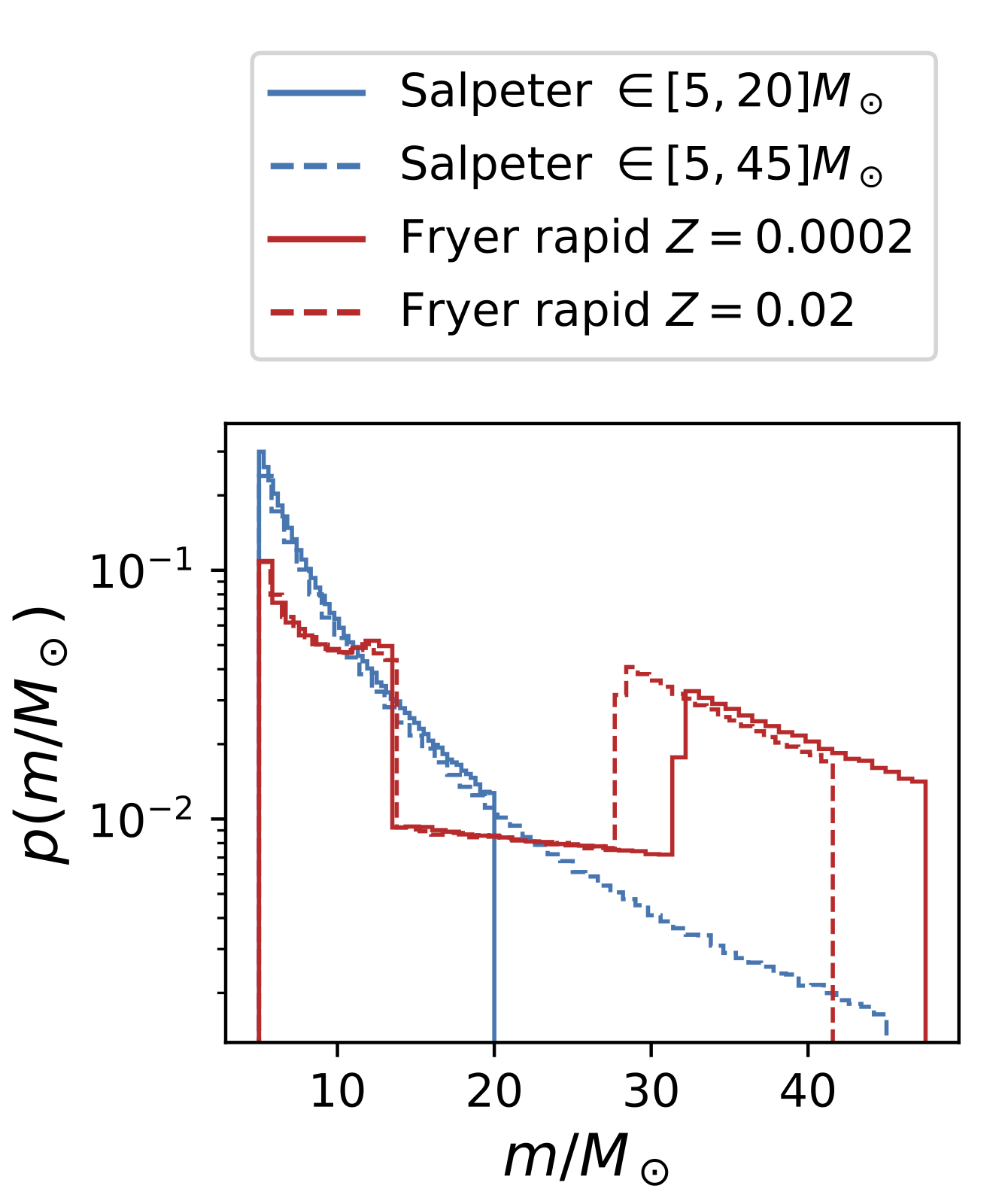
Figure 1: Four different scenarios for initial black hole mass distributions. Blue curves denote a Salpeter-like powerlaw, with the solid (dashed) line corresponding to an upper mass cutoff of $20M_{\odot}$ ($45M_{\odot}$). Red curves denote the Fryer rapid model, with the solid (dashed) line corresponding to a metallicity $0.0002$ ($0.02$).

The final ingredient we need to specify in our model is the initial distribution of masses and spins $f(x;t_{0})$. We hereafter refer to this as the “natal” distribution, and take it to be the distribution of black hole parameters formed at black hole birth. A variety of choices could be made, but here we restrict ourselves to two cases. The first case is a simple power-law mass function in component masses with lower and upper mass cutoffs

$$p(m)\propto\begin{dcases*}m^{-\alpha},&if $m_{\mathrm{min}}\leq m\leq m_{\mathrm{max}}$\\ 0,&otherwise.\end{dcases*}$$ (4)

In all cases we use the fiducial value $m_{\mathrm{min}}=5\,M_{\odot}$ for the sake of simplicity. For the other parameters, we either fix them to fiducial values of $\alpha=2.35$ (from a Salpeter IMF) and $m_{\mathrm{max}}=20\,M_{\odot}$ (from early stellar evolution modeling), or we allow the data to tune them, assuming uniform priors. The blue curves in Figure 1 show two examples of black hole natal mass distributions with the Salpeter prescription. The fiducial Salpeter mass distribution for black holes is a basic model which assumes that the fraction of mass retained from stellar birth to black hole formation, $m/m_{\mathrm{ZAMS}}$, is constant across all masses. This is unlikely to be true in reality, as the processes undergone by a star depend strongly on its mass. To take things a step further in complexity, we still assume the mass distribution follows a power law, but with an index $\alpha$ which differs from the IMF’s value. This is still fairly un-realistic, as the black hole natal mass spectrum is not expected to be this simple, but this at least lets the data determine the general trend of the spectrum.

Our second model has a better footing in physical principles, but loses some flexibility. We assume a pure Salpeter IMF for the ZAMS masses, in the range $[5,\infty)\,M_{\odot}$, and evolve them to black holes using the Fryer et al. (2012) Rapid model. (Our calculations implicitly adopt the same wind mass loss model as employed in that study.) This introduces an additional hidden variable, the stellar metallicity $Z_{\mathrm{metal}}$ for each progenitor star. The red and green curves in the bottom panel of Figure 1 show our inferred progenitor distributions, for two choices of $Z$. In principle, this should be a random variable, obeying some distribution which may correlate with the IMF. For simplicity, however, and motivated by the approximate similarity between these two distributions, we fix this to a constant $Z_{\mathrm{metal}}^{*}$, assumed to be the same for every progenitor.

Now we turn to to the black hole natal spins. Black hole natal spins remain a matter of considerable observational and theoretical debate. Motivated by LIGO’s observations and recent modeling (Fuller & Ma, 2019; Belczynski et al., 2017; Farr et al., 2018; The LIGO Scientific Collaboration & the Virgo Collaboration, 2018), we adopt a simple fiducial choice: all BHs in our original population have small characteristic spin magnitudes, drawn from a Beta distribution with ${\rm mean}(\chi)=0.047$ and ${\rm Var}(\chi)=0.002$. We also assume that the spin directions in the natal population are randomly oriented, but again we emphasize that other choices could be made.

2.3.4 Merger Rates

As described in §2.2, our Monte-Carlo procedure works with a finite set of black holes. We take these black holes to be a proxy for the entire population and assume that the overall merger rate of black holes is simply a scaled population of those generated in our Monte Carlo simulations. We also stipulate that the merger rate density is constant in co-moving volume. Future studies could certainly incorporate more detailed effects, but here we opt for simplicity. In the following section, we show normalized distributions of the masses and spins of black holes, but in §3 we present inference results that allow the merger rate density to be inferred by the data.

2.4 Characterizing the parameters

To elucidate the effect of each of the parameters described in the previous section, we take the reader through a sequence of examples. The examples we present here are primarily for illustration and do not necessarily represent parameters that describe the observed population of black-hole mergers to date. Note that the histograms and kernel density estimate curves shown here are not explicitly used in our analysis; they are simply representations of the samples from our Monte-Carlo procedure.

2.4.1 Time Evolution

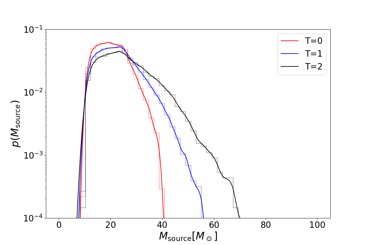
Figure 2: The total mass distribution of binary black hole mergers at three successive time steps evolving from a Salpeter natal distribution ($\alpha=2.35$) with coupling parameters $a=2$ and $b=0$. The smooth curves overlaid on the histograms are kernel density estimates of the Monte-Carlo samples and are shown purely to guide the eye.

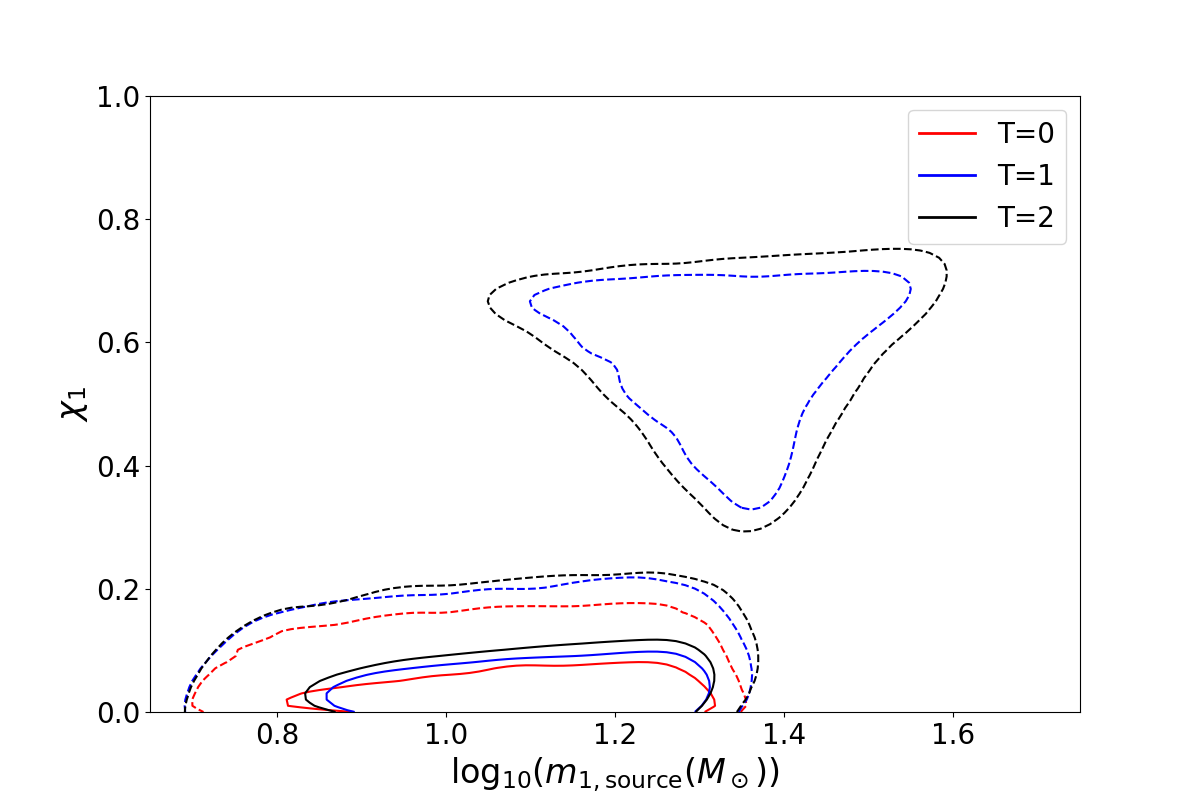
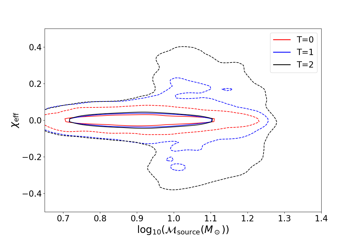
Figure 3: Joint mass-spin distributions for three successive time steps. Top: The spin amplitudes of the more massive merger component versus their masses. Bottom: The effective spin parameter $\chi_{\rm eff}$ versus the binary chirp mass. The contours represent 90% and 99.9% contour intervals for mergers at time steps $T=0$ (red), $T=1$ (blue), and $T=2$ (black).

As hierarchical mergers occur, a secondary population of high mass, high spin black holes begins to form alongside the natal population. In our Monte Carlo procedure, this time evolution of the population is reduced to individual time steps, as described in §2.2. Figure 2 illustrates how the population changes with each time step. Starting with a Salpeter IMF with $m_{\rm max}=20M_{\odot}$ and Beta-distribution spin magnitudes as the natal population (which we take as our fiducial natal population) we evolve the population forward for three iterations, allowing 5% of the black holes to merge at each step and setting the coupling strength to $a=2$ and $b=0$. The red, blue, and black lines show the distributions of the total masses of mergers for time steps 0, 1, and 2, respectively.

Since the remnant black holes inherit angular momentum from their parents and from their orbit, hierarchical mergers also produce strong evolution of BH spins (Fishbach et al., 2017; Gerosa & Berti, 2017). With successive mergers, the total mass distribution tends towards higher masses, and an island of high-mass, high-spin black holes begins to grow. Figure 3 shows 90% and 99.9% confidence intervals for the joint-mass spin distributions at $T=[0,1,2]$. Notably, hierarchical mergers of comparable-mass binaries introduce a characteristic peak near $\chi\simeq 0.7$, which is why the top panel of Figure 3 shows a surplus of black holes near that spin magnitude. Generically, hierarchical mergers should produce a similar subpopulation of high-mass, high-spin black holes, since general relativity predicts that a post-merger remnant black hole is always more massive than either of its pre-merger components and its final spin is away from zero. The $\chi_{\rm eff}$ versus chirp mass distribution in the lower panel shows that while $\chi_{1}$ tends to be large for the hierarchically produced mergers, the $\chi_{\rm eff}$ distribution is smoothed out around 0, since the black hole spin directions are isotropically distributed.

2.4.2 Coupling Strength

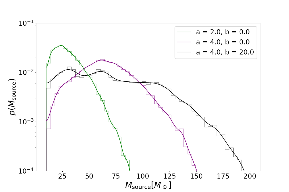
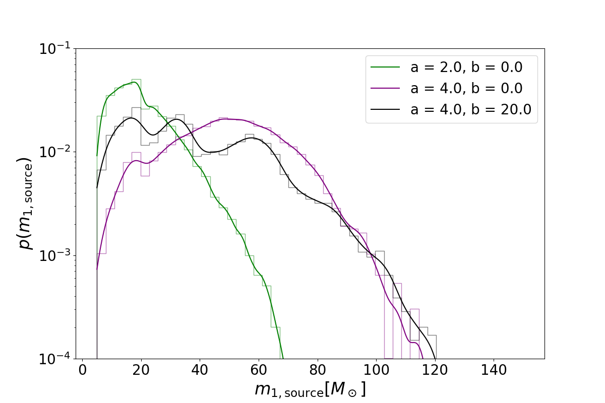
Figure 4: Mass distributions for different coupling parameters after four time steps. Top: The total mass distribution of mergers for $a=2,b=0$ (green), $a=4,b=0$ (purple), and $a=4,b=20$ (black). Bottom: The distribution of masses of the more massive merger components. The distributions are evolved from the fiducial Salpeter distribution.

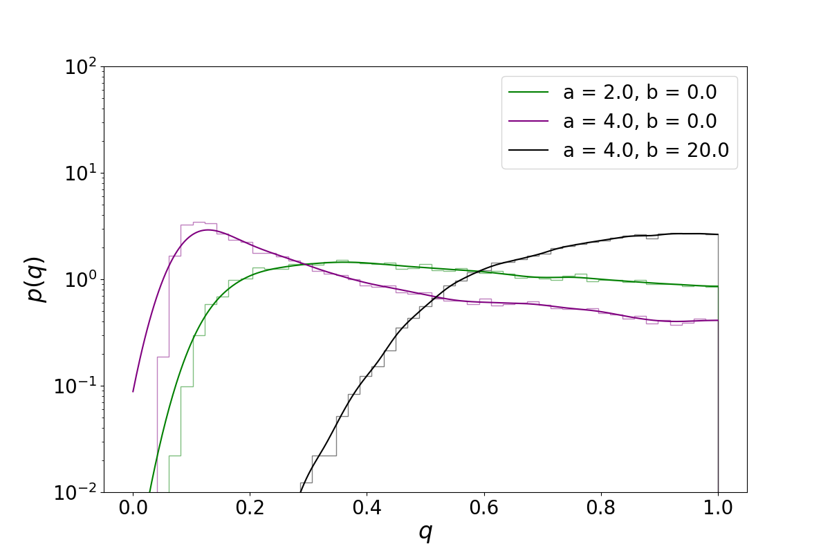
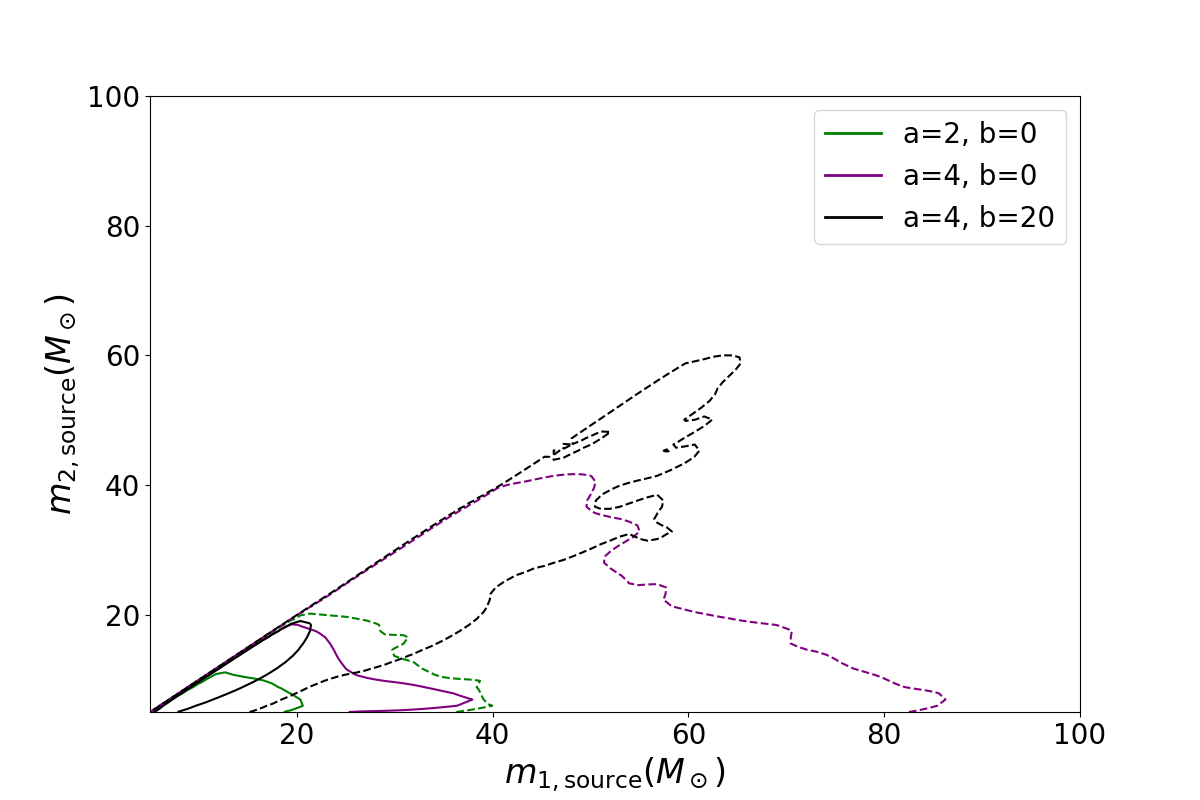
Figure 5: The distribution of mass ratios $q=m_{2}/m_{1}$ (top) and component masses (bottom) after four time steps for $a=2,b=0$ (green), $a=4,b=0$ (purple), and $a=4,b=20$ (black), evolved from our fiducial Salpeter distribution.

The overall mass and spin distributions are sensitive to the average coupling strength of black holes. Figure 4 shows the total mass distribution (top panel) and the primary mass distribution (bottom panel) after four time steps for different values of $a$ and $b$. Increasing the total mass coupling parameter $a$ drives the most massive mergers to occur, causing the total mass distribution to quickly expand to higher masses, while increasing the symmetric mass-ratio coupling $b$ simply forces most mergers to be of equal mass components. Cranking up $a$ and $b$ simultaneously gives particularly interesting behavior. In those cases, the heaviest black holes take place in mergers, and the products of those mergers are likely to merge again, which can create multiple distinct peaks in the mass distributions. As a result, in the Salpeter natal distribution example, our procedure produces a characteristic “smoothed staircase” mass distribution, with “steps” in the mass distribution appearing at multiples of the primordial maximum mass $m_{\mathrm{max},0}$. At very high mass, these “step” features become smoothed out.

The mass ratio and spin distributions also have characteristic features. When $a$ is large but $b$ is small, a population of highly unequal mass mergers can be produced, as seen in the purple curves of Figure 5. A near-flat mass ratio distribution (shown in green) is found for $a=2$ and $b=0$ in this case, because the natal mass distribution power law slope ($\alpha=2.35$) is nearly matched to the total mass coupling, so the dearth of higher mass black holes is exactly counteracted by their higher likelihood of participating in mergers. As $b$ is increased, the distribution begins to favor equal-mass mergers, as shown in the black curve.

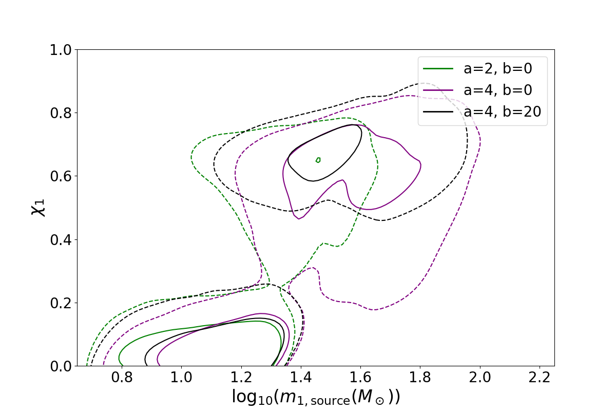
Figure 6: Contours of the joint $m_{1}$–$\chi_{1}$ distribution after four time steps for $a=2,b=0$ (green), $a=4,b=0$ (purple), and $a=4,b=20$ (black), evolved from the fiducial Salpeter distribution.

Figure 6 shows contours of the joint primary mass and $\chi_{1}$ distribution for different coupling strengths after four timesteps. While a high-mass, high-spin subpopulation is present in all the cases considered here, they are notably affected by the coupling strength parameters. When $b$ is large, the subpopulation is more concentrated at $\chi_{1}\sim 0.7$, because the mergers tend to be equal mass and therefore have a similar final remnant spin.

2.4.3 Depletion

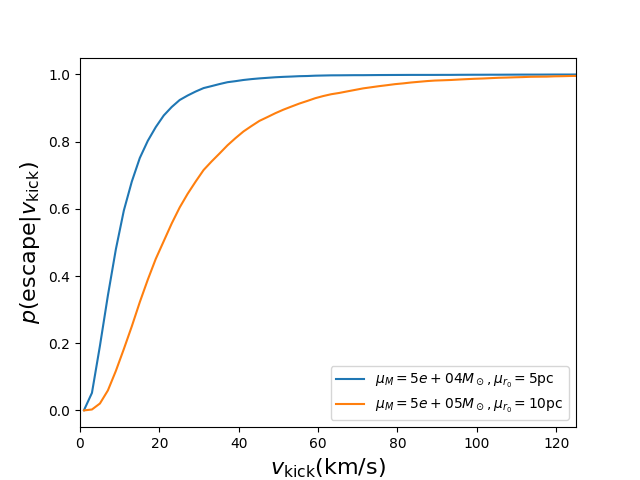
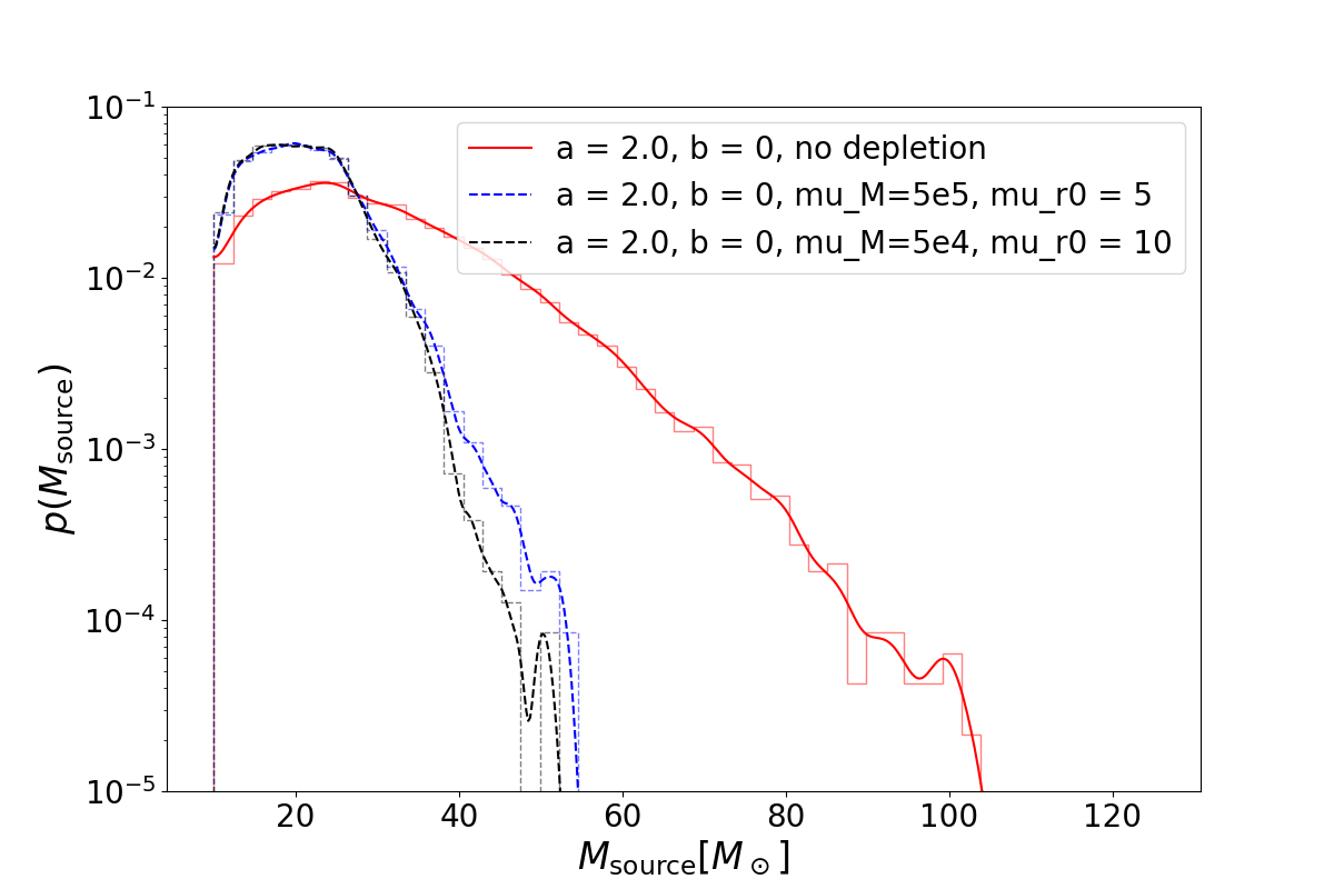
Figure 7: Escape probabilities and the total mass distribution of mergers for different depletion prescriptions. Top: The escape probability as a function of the kick velocity for “light” (blue curve, $\mu_{M}=5\times 10^{4}M_{\odot}$, $\mu_{r_{0}}=10$ pc, $\sigma_{M}=\sigma_{r_{0}}=1$) and “heavy” clusters (orange curve, $\mu_{M}=5\times 10^{5}M_{\odot}$, $\mu_{r_{0}}=5$ pc, $\sigma_{M}=\sigma_{r_{0}}=1$). Bottom: The total mass distribution for no depletion (red), “light” cluster depletion (black), and “heavy” cluster depletion (blue). The coupling parameters are set to $a=2,b=0$.

The most widely-proposed hierarchical scenario involves hierarchical formation in globular clusters. Merging black holes will be very frequently ejected from these low-binding energy environments, strongly suppressing the prospects for hierarchical mergers through multiple generations (Rodriguez et al., 2019; Gerosa & Berti, 2019; Favata et al., 2004; Merritt et al., 2004). To illustrate how depletion impacts the observed merger distributions, we incorporate the cluster depletion model from §2.3.2 into a hierarchical merger population. Figure 7 plots three total mass distributions, one without depletion effects, one with “light” clusters ($\mu_{M}=5\times 10^{4}M_{\odot}$, $\mu_{r_{0}}=10$pc, $\sigma_{M}=\sigma_{r_{0}}=1$), and one with “heavy” clusters ($\mu_{M}=5\times 10^{5}M_{\odot}$, $\mu_{r_{0}}=5$ pc, $\sigma_{M}=\sigma_{r_{0}}=1$). These hierarchical distributions are evolved forward four time steps from a fiducial natal distribution under these three depletion prescriptions and with $a=2,b=0$. This figure shows that as the confining potentials become shallower, remnant black holes are kicked from the environment so that hierarchical mergers are strongly suppressed, as known from previous work.

2.4.4 Natal Distributions

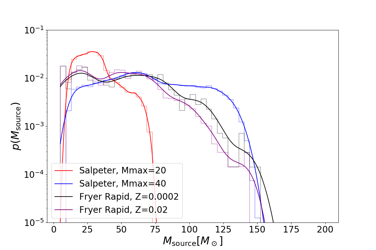
Figure 8: Total mass distributions after three time steps for different natal mass distributions. The coupling strength parameters are $a=4,b=20$.

As we have seen in the previous examples, the hierarchical distributions produced in our framework contain imprints of the natal populations. Figure 8 plots three hierarchical merger total-mass distributions after three time steps assuming the strong coupling parameters $a=4,b=20$. Unsurprisingly, the natal distributions with support at higher masses quickly evolve to have high-mass mergers. Additionally, the more complex structure in the Fryer natal mass distributions is imprinted in the evolved hierarchical distributions, while the Salpeter-based mass distributions are more smoothed out. In sum, the natal distribution is crucially important to the evolution of the mass distribution when hierarchical mergers can take place.

3 Constraining hierarchical formation with gravitational wave observations

We use an updated version of the PopModels population inference code (Wysocki et al., 2019) to compare our hierarchical formation model to real GW observations from GWTC-1 (The LIGO Scientific Collaboration & the Virgo Collaboration, 2019). For each collection of observations ${\cal D}$, this code evaluates the inhomogeneous Poisson likelihood

$$\mathcal{L}(\mathcal{R},\Lambda)\propto e^{-\mu(\mathcal{R},\Lambda)}\prod_{n=1}^{N}\int\mathrm{d}\lambda\,\ell_{n}(\lambda)\,\mathcal{R}\,p(\lambda\mid\Lambda),$$ (5)

where $\ell_{n}(\lambda)=p(d_{n}|\lambda)$ is the likelihood of data $d_{n}$ given binary parameters $\lambda$, $\mu(\mathcal{R},\Lambda)$ is the expected number of detections, $\mathcal{R}$ is the merger rate, and $\Lambda$ refers to any relevant model parameters: all parameters needed to characterize our hierarchical evolution equations, along with the choice of metallicity and initial conditions. Unlike Wysocki et al. (2019), we evaluate the integrals $\int d\lambda\ell_{n}(\lambda)p(\lambda|\Lambda)$ by using Monte Carlo integration via samples drawn from our hierarchical model $p(\lambda|\Lambda)$, combined with an analytic likelihood $\ell_{n}(\lambda)$.

Table 1: Hierarchical Merger Models Fit to O1/O2 Data

Model	Description
Model 1	Natal population: power-law in component mass • $m_{\rm min}=5M_{\odot}$ • $\alpha\in[-3,5]$, uniform • $m_{\rm max}\in[15,50]$, uniform • $\mathbb{E}[\chi]=0.047$ • ${\rm Var}[\chi]=0.002$ Coagulation parameters: • $a\in[1,6]$, uniform • $b\in[1,100]$, log uniform • $T\in[0,9]$, uniform • $w=0.05$
Model 2	Same as Model 1, except $T\in[0,5]$ and • Beta distribution natal spins – $\mathbb{E}[\chi]\in[0,1]$, uniform – ${\rm Var}[\chi]\in[0.25]$, uniform • Depletion – $\mu_{M}=5\times 10^{5}M_{\odot}$ – $\mu_{r_{0}}=5$ pc – $\sigma_{M}=\sigma_{r_{0}}=1$
Model 3	Same as Model 2 except • $\mu_{M}\in[10^{5},10^{10}]M_{\odot}$, uniform • $\mu_{r_{0}}\in[5,5^{5}]$ pc, uniform
Model 4	Mixture of Model 2 and Model A of The LIGO Scientific Collaboration & the Virgo Collaboration (2018)
Model 5	Same as Model 1 except • Fryer rapid SN natal population • Mixture with Model A of The LIGO Scientific Collaboration & the Virgo Collaboration (2018) • $T=2$

We perform inference with four models, which are described in Table 1. The right hand side describes prescriptions for fixed values and priors in each model. The posterior distributions on our inference parameters are shown in Figures 9, 10, and 11. Model 1 is our most basic phenomenological model, with a power-law-in-component-mass, zero spin natal distribution. The number of iterations and mass coupling parameters are inferred from the data. The blue curves in the right panel of Figure 9 show that the data have a slight preference for $a\sim 2$ and a strong preference for large $b$ values around $b\sim 30$. The overall rate density of mergers in our hierarchical model $\mathcal{R}_{\mathrm{h}}$ shown in the left panel, is consistent with the rates inferred in The LIGO Scientific Collaboration & the Virgo Collaboration (2018). Additionally, the natal distribution power law index and maximum mass are constrained to similar values to those found in The LIGO Scientific Collaboration & the Virgo Collaboration (2018), as seen in the blue curves of Figure 10. Given that our hierarchical model reduces to a non-hierarchical model in the low-timestep limit and the data favors fewer time steps, it is not surprising that our natal population parameters match the overall population parameters in The LIGO Scientific Collaboration & the Virgo Collaboration (2018). The inference on the number of time steps is shown in Figure 9 in terms of the variable $N_{\rm gen}=T+1$, which is the highest allowed generation of black holes in the population.

The most widely-proposed hierarchical scenario, however, involves hierarchical formation in globular clusters. Merging black holes will be very frequently ejected from these low-binding energy environments, strongly suppressing the prospects for hierarchical merger (Rodriguez et al., 2019; Gerosa & Berti, 2019). Model 2 adds a depletion prescription to Model 1 with fixed cluster mass and radius distribution parameters. In this case, similar coupling and natal distribution parameters to Model 1 are inferred, which is shown in orange in Figures 9 and 10. Notably there is a slight preference for higher total mass couplings $a$ for Model 2 compared to Model 1, because the depletion effects strongly suppress hierarchical mergers and therefore higher masses from the natal population are favored. The strong depletion in this case also results in no preference on the number of time steps.

We then allow the cluster mass and radius distribution parameters to vary in Model 3. The results of inferring cluster sizes are shown in Figure 11. Interestingly, the cluster radii and masses are pushed to large values, far greater than those of real star clusters. This is partially an artifact of the parameterization chosen here. The gravitational potential in the Plummer profile is sensitive only to the ratio of cluster mass to cluster radius, so if we consider the ratios of $\mu_{M}$ to $\mu_{r_{0}}$, the inferred values are roughly similar in gravitational potential to the fixed values used in Model 2. In other words, the data prefer somewhat shallow potentials wherein hierarchical mergers are suppressed. A future parameterization may instead opt for a distribution of gravitational potentials rather than cluster parameters.

Next we consider two mixture models. In the first (Model 4), we fit a mixture of our Model 2 with Model A from The LIGO Scientific Collaboration & the Virgo Collaboration (2018). Then in Model 5 we create a mixture of Model A and our hierarchical model applied to the the Fryer rapid SN natal population with no depletion and exactly 3 timesteps of evolution. In these mixture analyses, we simultaneously fit the parameters of Model A (power-law index, maximum mass cutoff, overall rate) and the parameters of the hierarchical model. Figure 10 shows the distributions of population parameters for the “field” (Model A) and “hierarchical” mixtures. The mixtures complicate the picture significantly. Model 4 (shown in red) in particular has little discerning power on its underlying population parameters due to the additional model freedom. Model 5 (purple) on the other hand, for which the natal distribution and number of time steps are fixed, shows some interesting behavior. In particular, the “field” (i.e. Model A) component parameters are driven to a near flat distribution in component masses with a slightly lower mass cutoff than for the other models considered inferences. Meanwhile, the coagulation parameters $a$ and $b$ are pushed to lower values. These shifts in the inferred parameters are likely due to fixing the number of timesteps to 3 with no depletion. Fixing the number of timesteps to 3 favors the existence of some hierarchical mergers which tend to be higher mass. To counteract the build up of too many high-mass black holes compared to the data, the mass distribution of the field population is cut off at a lower $m_{\rm max}$ and the coagulation mass coupling is decreased. Also, the inferred metallicity $Z_{\mathrm{m}}$ of the natal population also slightly favors higher values, which pushes the natal mass distribution to lower masses, alleviating some of the unwarranted build-up of high mass black holes. Lastly, the contribution of the hierarchical population is subdominant to the field population, as seen in Figure 11.

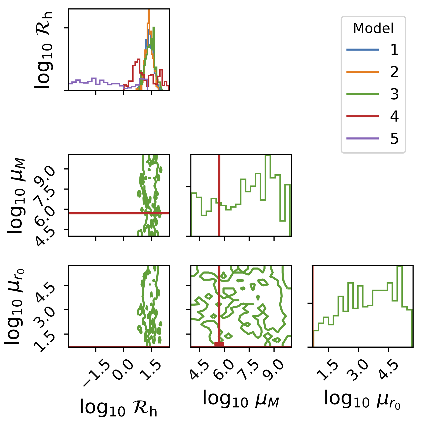
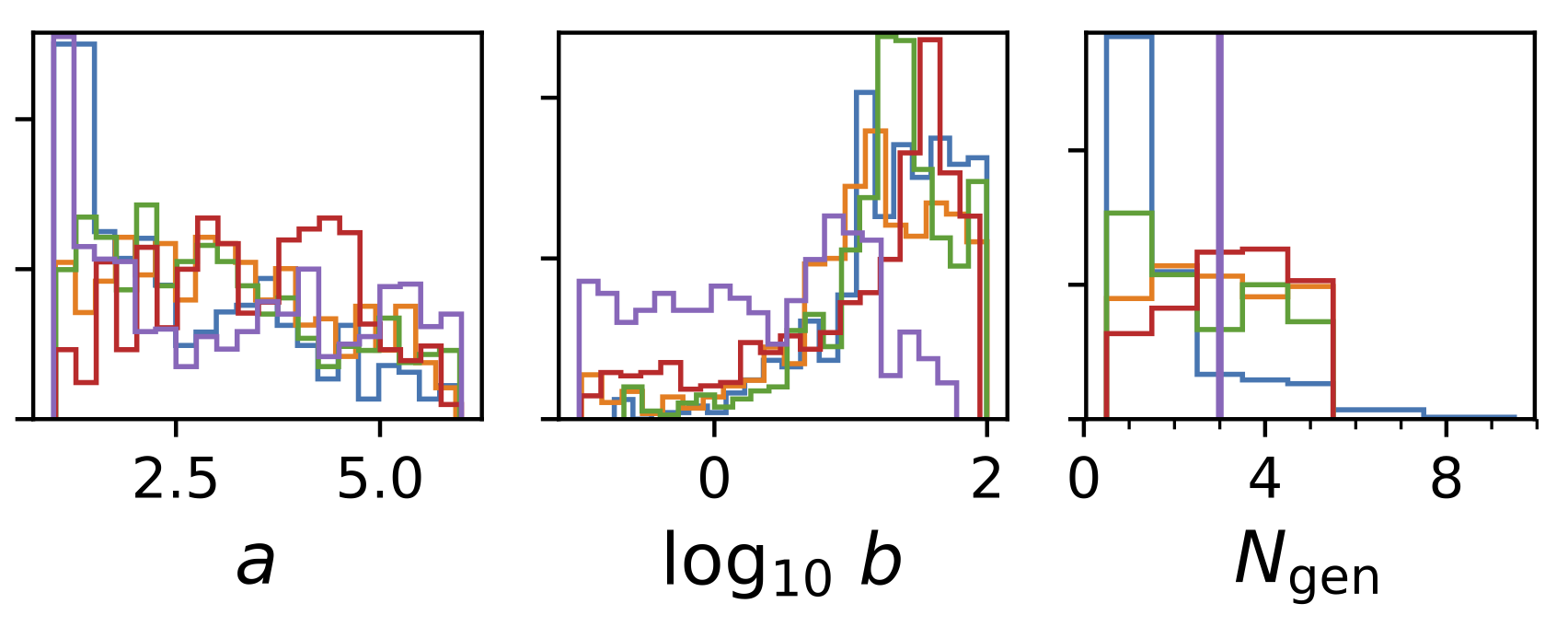
Figure 9: Inferred hierarchical parameters with depletion effects, for the 5 models listed in Table 1. Top: Hierarchical merger rates and cluster parameters for hierarchical mergers with depletion effects considered. Note that the fiducial model, based on globular clusters vastly underestimates the inferred cluster scales. Bottom: Merger cross section indices for $\Gamma\propto M^{a}\,\eta^{b}$, for different models both with and without depletion. Note that the only significant difference comes from using the Fryer natal population.

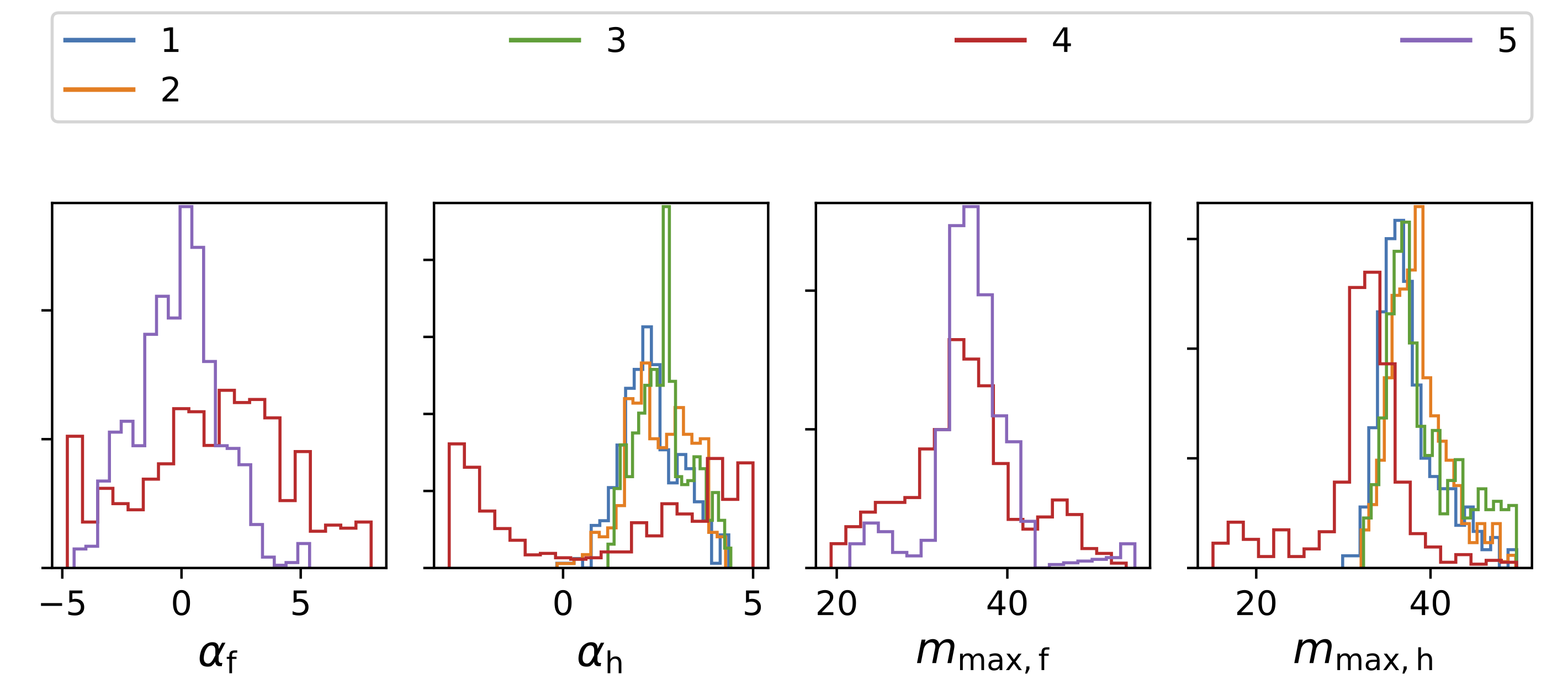
Figure 10: Impact of depletion on powerlaw parameters. Field and hierarchical components are denoted with $\mathrm{f}$ and $\mathrm{h}$ subscripts, respectively.

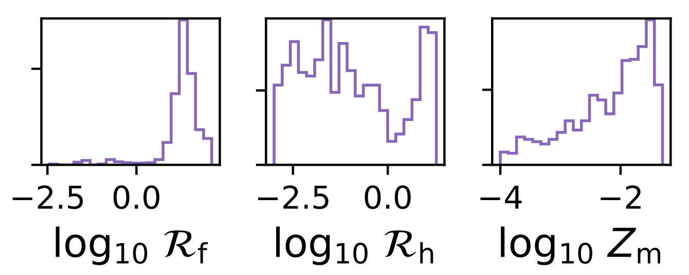
Figure 11: Inferred rates and metallicities for model 5. We infer merger rates for both the hierarchical component ${\cal R}_{\mathrm{h}}$ and the non-hierarchical component ${\cal R}_{\mathrm{f}}$.

4 Discussion

A hierarchical formation scenario provides an efficient way to produce binaries which would otherwise be challenging to generate: high masses, exceptional mass ratios, and characteristically high spins. The identification of binaries with characteristically extreme properties could provide a clear indication of hierarchical formation. In this section we explore our posterior predictive constraints on these scenarios, within the framework of the constrained fiducial model described above. We also discuss further extensions of the models presented here and the overall effectiveness of this framework.

4.1 Posterior Predictive Distributions

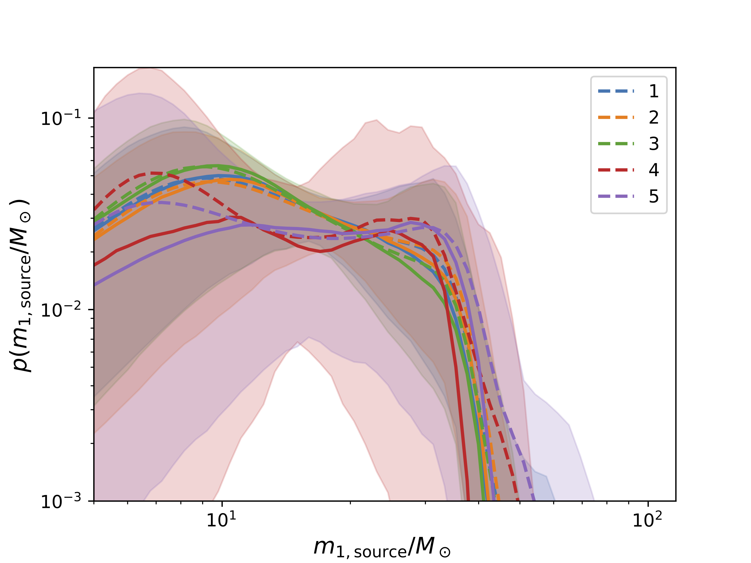
Figure 12: Inferred $m_{1,\mathrm{source}}$ distributions for Models 1-5. Shown are the median (solid line), posterior predictive (dashed line), and 90% credible intervals (shaded region).

Figure 12 shows our inferred posterior mass distribution, both intrinsic and detection-weighted, which resemble the conclusions in The LIGO Scientific Collaboration & the Virgo Collaboration (2018). Specifically, we infer a mass distribution for the more massive component in merging black holes ($m_{1}$) that is approximately a power law between $10M_{\odot}$ and $30M_{\odot}$, followed by a rapid decrease at higher mass. Notably, this figure shows characteristic decay and “echo” features at about $30M_{\odot}$, inherited by our formation model; these features could be probed by future observations and used to better constrain hierarchical formation.

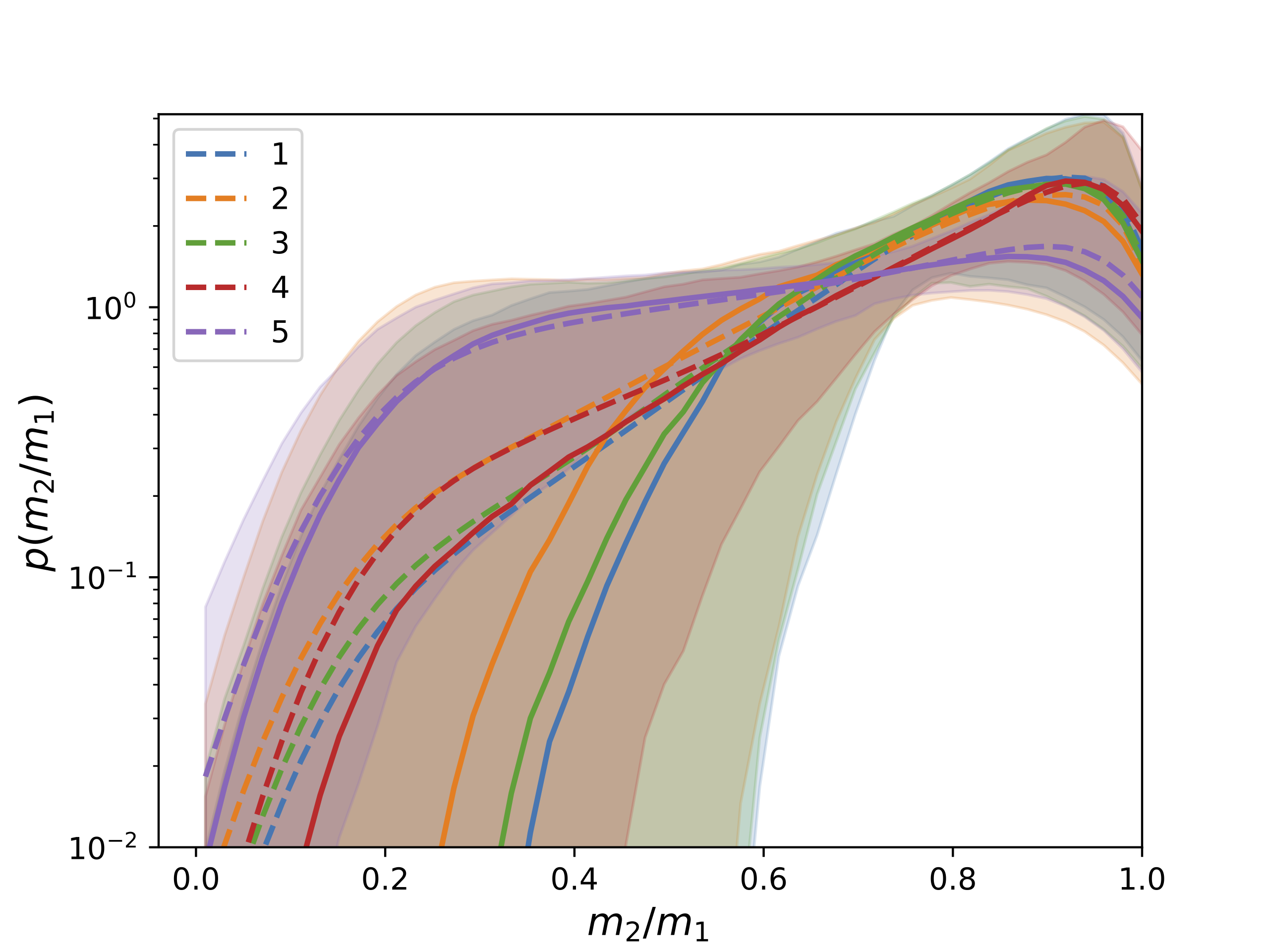
Figure 13: Inferred $m_{2}/m_{1}$ distributions for Models 1-5. Shown are the median (solid line), posterior predictive (dashed line), and 90% credible intervals (shaded region).

Figure 13 shows our inferred mass ratio distribution. Because GWTC-1 does not include a significant component of asymmetric binaries, our posterior necessarily strongly favors hierarchical models which preferentially produce binaries with $q\simeq 1$. Constraints on binary mass ratios will very strongly constrain prospects for hierarchical formation, particularly insofar as some hierarchical scenarios produce significant numbers of highly asymmetric mergers (Yang et al., 2019).

4.2 Possible Extensions

In this article, we have shown a few possible model choices and prescriptions, but as we have emphasized, many other choices could be made. For example, our parameterizations of the coagulation coupling and cluster depletion are essentially phenomenological, but future work could incorporate the results of N-body simulations which evolve clusters of stars and black holes as well as incorporate observational constraints on star clusters.

Our current parameterization also assumes that there is no evolution of the rate or mass and spin distributions with redshift. Given the evolution of the cosmic star formation rate, it is likely that the rate of black hole mergers is increasing between $z=0$ to $z\sim 1$, and analysis of available gravitational wave data has already lent weak support to that hypothesis (Fishbach et al., 2017; The LIGO Scientific Collaboration & the Virgo Collaboration, 2018). Additionally, properties of the environments in which black holes merge (such as the distribution of cluster potentials) could have changed over cosmic time, leading to observable differences in the mass and spin distributions between low and high redshifts.

Another possible extension to our model would be to consider more complex mixtures of populations. We briefly considered a “field” plus “cluster” mixture population here, but if mergers are occurring in AGN disks, globular clusters, in the field, and from a primordial population, more mixture components would need to be added. More gravitational-wave data will be needed before embarking on such investigations, as the number of parameters of such a complex mixture will proliferate.

Lastly, we note that this work has not considered neutron stars. After this work reached maturity, we became aware of a similar investigation targeting hierarchical formation of neutron stars (Gupta et al., 2019). Nevertheless, our framework could neatly incorporate neutron stars by substituting in a neutron-star natal distribution and a model for neutron-star merger remnant masses, spins, and kick velocities. The main new addition in a hierarchical population based on NS mergers would be the need to incorporate an equation of state.

4.3 Efficacy of this Hierarchical-Merger Population Framework

Our phenomenologically-parameterized framework provides an efficient way to characterize the contribution of hierarchical mergers to a compact binary population, and to interpret BH mass measurements as constraints on this sub-population. We can use GW measurements to infer the natal mass and spin distribution, as well as evolution parameters. Of course, our model cannot completely disambiguate these two features without other observational or physical input. As a trivial example, any set of GW observations can be explained by a non-hierarchical population and a suitably-overfit natal mass and spin distribution. If, however, physical constraints limit the flexibility of the natal BH binary distribution to populate parts of parameter space, then the presence of merging BHs in those distinctive regions provides evidence for hierarchical formation. In such a scenario, our framework enables us to provide first constraints on a hierarchical merger interpretation.

In this work, motivated by LIGO’s observations in GWTC-1, we have emphasized formation scenarios with strong effective coupling, to produce a binary black hole population which favors comparable-mass mergers. We expect that more theoretically-motivated choices for these interaction exponents will favor a wider range of mass ratios. As noted in previous work (McKernan et al., 2019), high mass ratio binaries could be a distinctive signature of certain hierarchical growth scenarios. The presence or absence of high mass or high-mass ratio binaries strongly constrains our model parameters and the overall hierarchical merger rate.

Another characteristic feature of some hierarchical merger scenarios is a “smoothed staircase” or multi-modal pattern in the mass distributions. In the simplest case where the natal population is just composed of black holes with mass $M_{\rm natal}$, “harmonics” of the natal mass should appear in the black hole mass spectrum at multiples $M_{\rm natal}$. If the natal distribution is sufficiently complex, such harmonics may be blended out, but as shown in 2, there are intermediate cases where smoothed out harmonics or “staircases” are still noticeable.

Conversely, many mass and spin distributions cannot be naturally produced from hierarchical evolution. If hierarchical formation is proposed to explain a subpopulation of high-spin or high-mass or high-mass ratio binaries, then the relative merger rate of this feature is often bounded above. For example, we would need sufficient numbers of low-mass BHs to explain a population of high-mass, high-spin BHs entirely through hierarchical formation.

Once an observed population is fit with a realization of a hierarchical population, our Monte Carlo method enables computation of some interesting quantities. In principle, each Monte Carlo sample has an associated “family tree” which tracks successive mergers that the black hole had previously undergone. Thus one can evaluate the probability that a given black hole was hierarchically formed and underwent $n$ previous mergers. Alternatively, upper limits can be set on the rate of hierarchical mergers if none are suspected in the GW sample.

5 Conclusions

Observing hierarchically formed black holes is an exciting prospect for gravitational-wave detectors. We have presented here a self-consistent framework for generating black-hole merger populations that includes hierarchical formation. This framework evolves arbitrary natal black hole populations, enabling any existing black hole distributions to be extended to include hierarchical mergers. With the cases we explore here, our fits suggest that scenarios with many hierarchical mergers are disfavored.

In this work, we simulated coagulation and depletion effects while assuming the binary black hole population is not continuously repopulated from another reservoir of black holes. We will explore self-consistent repopulation in later work. We also perform simplified averaging, not allowing for a distribution of initial conditions like metallicity or for trends versus redshift. Our scheme ignores higher order correlations and multi-body effects, thus averaging everything into an effective cross section which is constant. Our approximation is reasonable in the limit of weak hierarchical reprocessing dominated by a low-mass seed population; we defer more sophisticated averaging to future work. Additionally, we adopt a simple dependence of $\Gamma$ on total mass, allowing it to increase without bound according to a single power law as the binary mass increases. More detailed investigations will produce more complex dependence of $\Gamma$ on mass. The results of our inference on GWTC-1 with partially constrained versions of our model framework show consistency with The LIGO Scientific Collaboration & the Virgo Collaboration (2018), but more detections are required to make more definitive statements about whether hierarchical formation of black holes is at work. Our fits to GWTC-1 hint that hierarchical merger scenarios are not required to fit the population, but are also not ruled out by the population. However, the conclusions drawn herein are subject to the simplifying assumptions made for this preliminary analysis. Incorporation of more astrophysically motivated inputs to the framework will be necessary to put the tightest constraints on the formation environments and scenarios. With the wealth of black hole merger detections we expect to see in the coming years, the prospects for uncovering hierarchically formed black holes are promising, and the framework we have presented herein is well-suited for such investigations.

The general purpose hierarchical population code will be released for public use in the near future.

Appendix A Semianalytic approach to hierarchical mergers

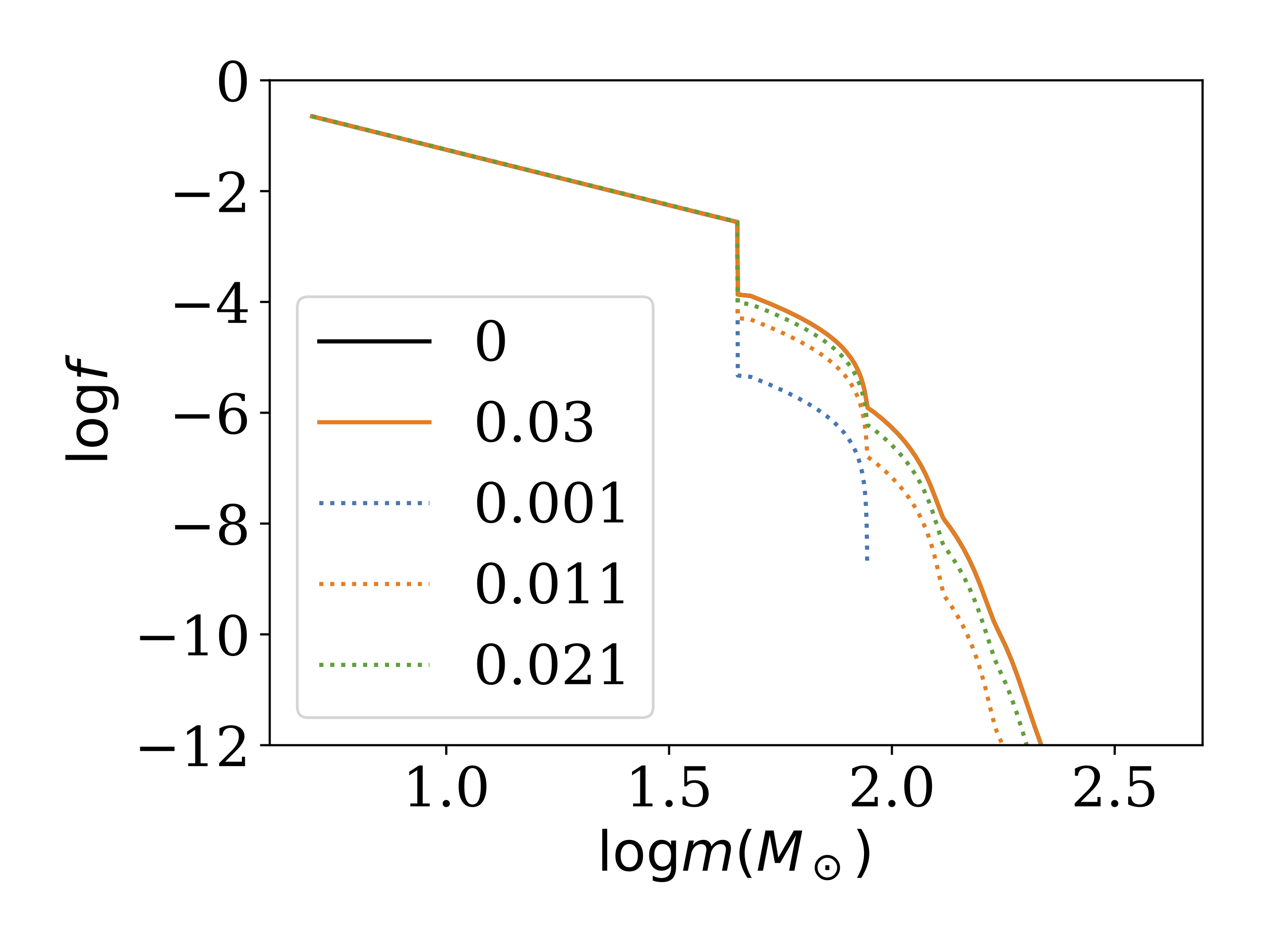
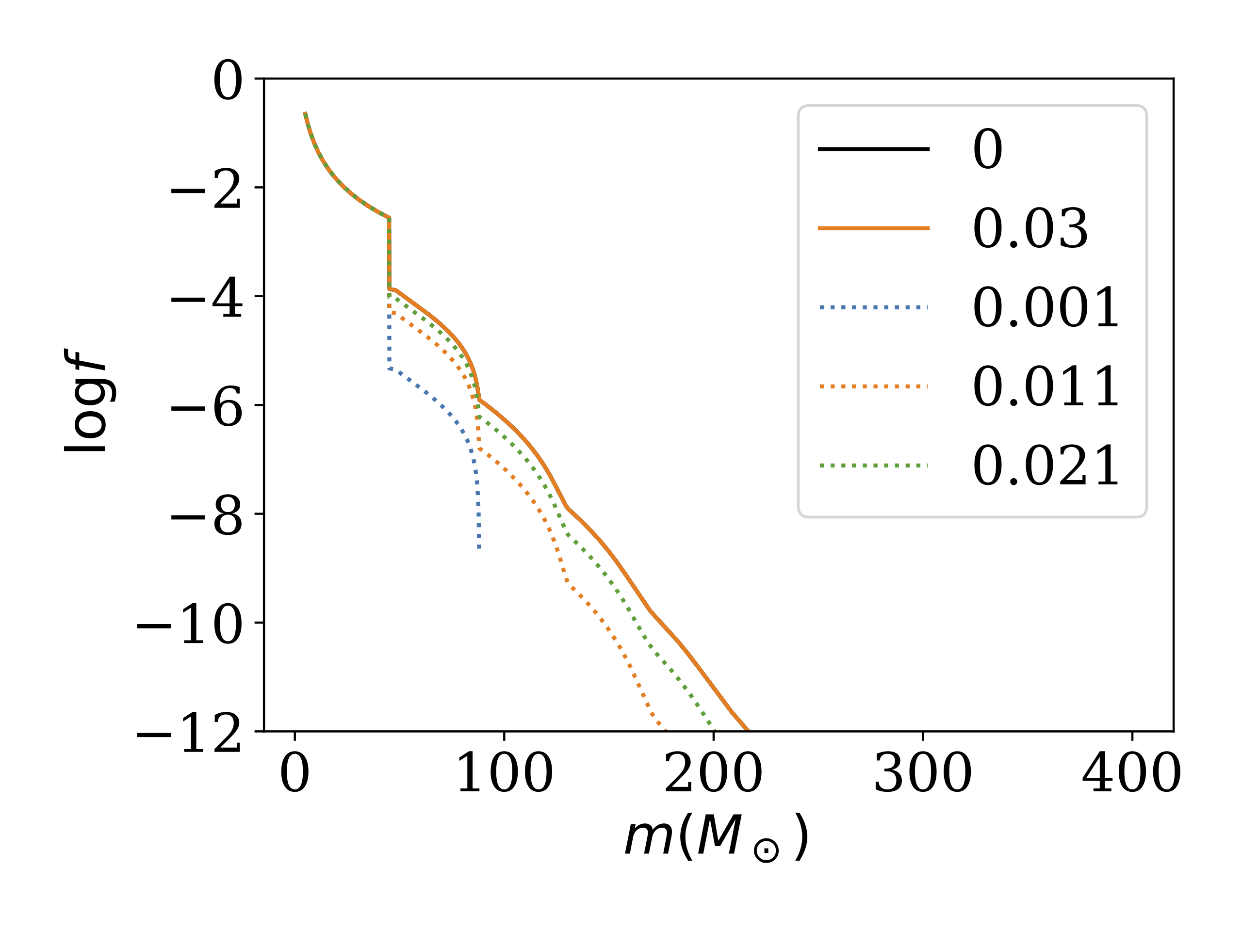
Figure 14: Synthetic mass distribution as a function of $x$ due to hierarchical mergers with $a=2,b=0$ and no depletion, starting with a truncated power law distribution at $x=0$. Colors and legend denote different choices for $x$. Bottom panel uses a log-linear scale to highlight exponential decay at large mass.

In the text, we consistently employ a concrete Monte Carlo implementation of hierarchical mergers. This powerful method allows us to efficiently incorporate the best merger physics, but uses discrete generations. In this appendix, for pedagogical purposes we provide a toy model implementation of a true continuous-time coagulation equation. In this approach, we consider only the evolution of binary mass, assuming no mass is lost during mergers; we neglect spins and depletion. After these simplifications, our model is essentially analytically tractable, and can be understood by both perturbation theory and direct numerical simulation. In this appendix, we present a few supplementary illustrations of these hierarchical calculations, to further illuminate our model’s behavior at very high mass and in the absence of depletion.

As our first example, to illustrate the parameters $\zeta$ and $a$, Figure 14 shows the results of evolving Eqs 1 starting with an initial power law mass distribution through different ranges of interaction parameter $\zeta\ll 1$, for two choices of $a$ and for $b=0$. The dotted curves show the results of a direct numerical time integration; the solid curves show our Monte Carlo procedure; and different colors indicate different choices for $x$ and $a$ respectively.

This example first shows how the parameter $\zeta$ controls the effective number of generations at the reference parameters, absorbing factors present in the overall interaction time $T$ and in the interaction cross section $\Gamma$. As expected based on perturbative arguments, higher-order generations increase in significance in proportion to $x^{g}$ for $g$ the number of generations. At very high mass, the hierarchical mass distribution approaches an exponentially decaying function of $m$, which increases exponentially with $x^{2}$.

Second, this example shows how the coagulation equation successively reprocesses each generation, potentially with different interaction scales. In this example and generally in the usual case that $a,b>0$, binaries with smaller masses or more asymmetric mass ratios by construction interact even less frequently. Conversely, within our framework high mass binaries rapidly undergo multiple generations of mergers. As a result, in this power law example, our procedure produces a characteristic “smoothed staircase” mass distribution, with “steps” in the mass distribution appearing at multiples of the primordial maximum mass $m_{max,0}$. At very high mass, these “step” features become smoothed out.

Third, this example shows the importance of the interaction cross section: because we adopt $b=0$ (no preference to any mass ratio) and because low-mass BHs are dramatically more prevalent than high-mass binaries, the overall merger rate $f(x)f(x^{\prime})\Gamma_{x,x^{\prime}}$ for binaries with one massive component $x$ is overwhelmingly dominated mergers where $x^{\prime}$ is drawn from this scenario’s ubiquitous low-mass black holes. As a result of these frequent minor mergers, features in the mass spectrum proportional to the primordial maximum mass are rapidly smoothed out, both in $x$ and as we go to higher multiples of the maximum mass, except for the first feature.

In sum, our coalgulation model naturally “builds up” self-consistent hierarchical populations, producing mass distributions which can (but need not) possess clear features reflecting the number of generations and any sharp cutoffs present in the seed distribution.

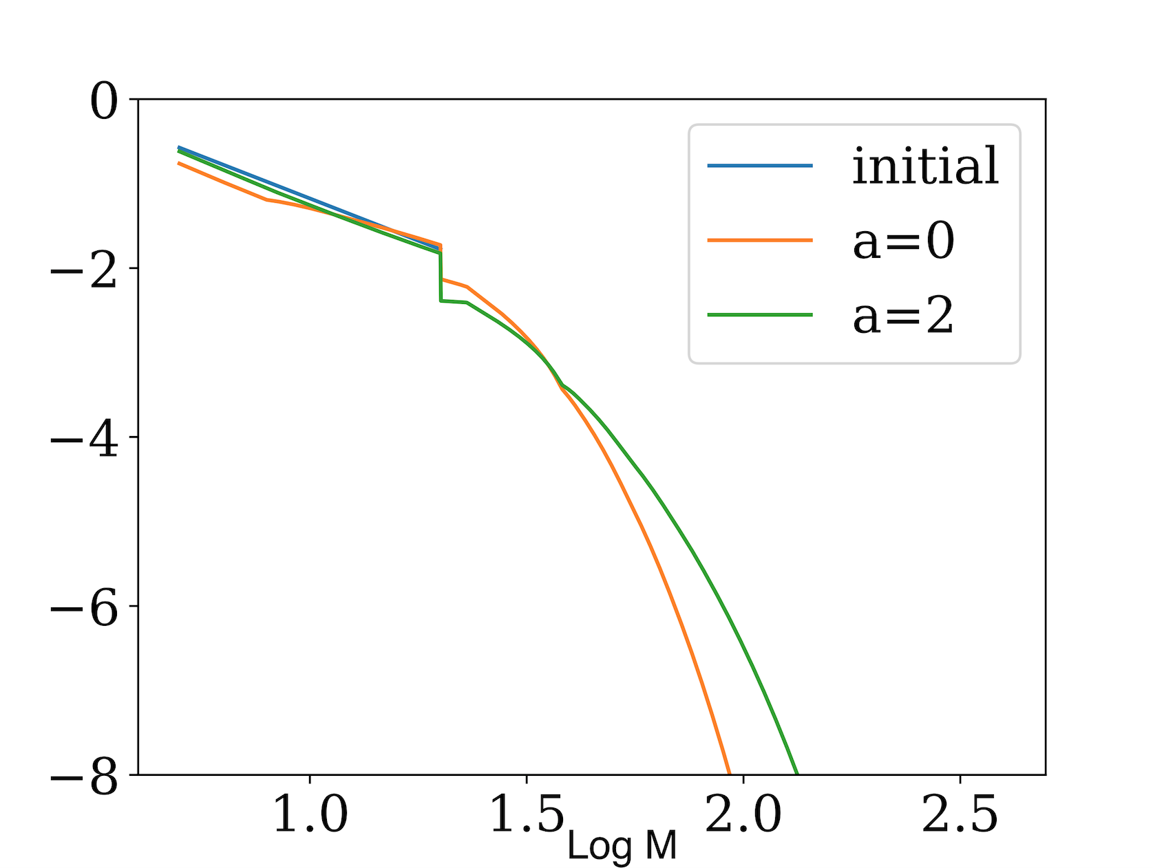
Figure 15: Illustration of the evolving mass distribution: logarithm of the mass spectrum versus mass.

As our second example, we consider how features of the high-mass mass distribution are inherited from the low-mass mass spectrum., using a broad, featureless power law distribution initially $f(m)\propto m^{-\alpha}$ at low mass. For simplicity and unlike the example used above, we consider interactions with $b\gg 1$, insuring that almost all mergers occur between comparable-mass binaries.

Qualitatively speaking, coagulation requires the formation rate of BHs with mass $2m$ must be $\Gamma f(m)^{2}\propto m^{a-2\alpha}$, a slope which can be shallower or steep than the low-mass slope $(-\alpha)$ depending on the sign of $a-\alpha$. Evidently, as corroborated by Figure 15, larger $a$ favors higher-mass black holes and a more extended tail in the mass distribution. As in the previous example, at very high masses the distribution decays exponentially, with a coefficient that depends on $a$.

Appendix B Changing the merging fraction

Rather than use a continuous-time coagulation equation, which implicitly allows BH remnants to participate in subsequent hierarchical mergers immediately, we employ discrete timesteps with a specific fraction $w$ of BHs that participate in mergers at each iteration. As $w\rightarrow 0$, our algorithm converges to continuous coagulation, because the population changes slowly over many iterations, ensuring that $\Delta f(x,t)/\Delta t$ is small at each step and that post-merger remnant black holes are immediately available to merge again. As $w$ increases, our iterative process increasingly differs from continuous evolution. In effect, $w$ encodes a “recycling delay time,” i.e. the time for a post-merger remnant black hole to be re-integrated into the population. We emphasize that while larger $w$ loses fidelity to the continuous coagulation equation, high $w$ can still model a real compact object population. For example, it is conceivable that all natal black holes merged at an early time (i.e. $w$=1), and then all participate in second generation mergers at later times.

As a concrete example, we apply our algorithm to our fiducial power-law natal population using different $w$ values while holding constant the total number of mergers. In other words, we ensure $wT$ is a constant, where $T$ is the number of iterations of our Monte Carlo method. The coupling constants $a$ and $b$ are set to 0. Figure 16 shows the total mass distribution of mergers after $T=2,4,8,16$ iterations with $w=0.08,0.04,0.02,0.01$, respectively. At lower masses, the distributions roughly agree, but only the small $w$ cases have tails extending to higher masses, since those cases are closer to continuous coagulation wherein there is no recycling delay time and post-merger remnants are free to re-merge immediately.

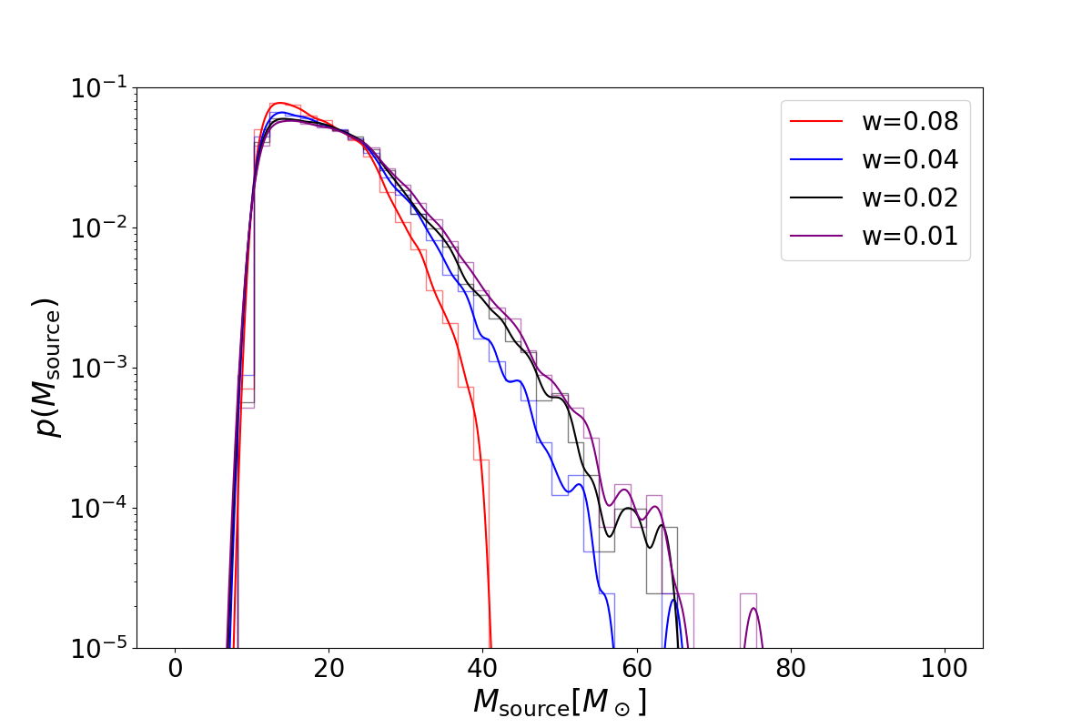
Figure 16: The total mass distribution for different fractions of mergers per time step. The number of time steps $T$ is varied such that the total number of mergers is constant. Specifically, $T=2,4,8,16$ for $w=0.08,0.04,0.02,0.01$, respectively.

References

- Accadia & et al (2012) Accadia, T., & et al. 2012, Journal of Instrumentation, 7, P03012. http://iopscience.iop.org/1748-0221/7/03/P03012
- Antonini & Rasio (2016) Antonini, F., & Rasio, F. A. 2016, ApJ, 831, 187, doi: 10.3847/0004-637X/831/2/187
- Bartos et al. (2017) Bartos, I., Kocsis, B., Haiman, Z., & Márka, S. 2017, ApJ, 835, 165, doi: 10.3847/1538-4357/835/2/165
- Belczynski et al. (2017) Belczynski, K., Klencki, J., Meynet, G., et al. 2017, Submitted to Astron.& Astrophysics (arXiv:1706.07053). http://xxx.lanl.gov/abs/arXiv:1706.07053
- Belotsky et al. (2019) Belotsky, K. M., Dokuchaev, V. I., Eroshenko, Y. N., et al. 2019, European Physical Journal C, 79, 246, doi: 10.1140/epjc/s10052-019-6741-4
- Breivik et al. (2016) Breivik, K., Rodriguez, C. L., Larson, S. L., Kalogera, V., & Rasio, F. A. 2016, ApJ, 830, L18, doi: 10.3847/2041-8205/830/1/L18
- Chatziioannou et al. (2019) Chatziioannou, K., Cotesta, R., Ghonge, S., et al. 2019, Submitted to PRD, available as arxiv:1903.06742; see also https://dcc.ligo.org/LIGO-T1900096/public
- Christian et al. (2018) Christian, P., Mocz, P., & Loeb, A. 2018, ApJ, 858, L8, doi: 10.3847/2041-8213/aabf88
- Clesse & García-Bellido (2015) Clesse, S., & García-Bellido, J. 2015, Phys. Rev. D, 92, 023524, doi: 10.1103/PhysRevD.92.023524
- Clesse & García-Bellido (2017) —. 2017, Physics of the Dark Universe, 15, 142, doi: 10.1016/j.dark.2016.10.002
- Collete (2013) Collete, A. 2013, Python and HDF5 (O’Reilly)
- Farr et al. (2018) Farr, B., Holz, D. E., & Farr, W. M. 2018, ApJ, 854, L9, doi: 10.3847/2041-8213/aaaa64
- Favata et al. (2004) Favata, M., Hughes, S. A., & Holz, D. E. 2004, ApJ, 607, L5, doi: 10.1086/421552
- Fishbach & Holz (2019) Fishbach, M., & Holz, D. E. 2019, arXiv e-prints, arXiv:1905.12669. https://arxiv.org/abs/1905.12669
- Fishbach et al. (2017) Fishbach, M., Holz, D. E., & Farr, B. 2017, ApJ, 840, L24, doi: 10.3847/2041-8213/aa7045
- Fryer et al. (2012) Fryer, C. L., Belczynski, K., Wiktorowicz, G., et al. 2012, ApJ, 749, 91, doi: 10.1088/0004-637X/749/1/91
- Fuller & Ma (2019) Fuller, J., & Ma, L. 2019, ApJ, 881, L1, doi: 10.3847/2041-8213/ab339b
- Gerosa & Berti (2017) Gerosa, D., & Berti, E. 2017, Phys. Rev. D, 95, 124046, doi: 10.1103/PhysRevD.95.124046
- Gerosa & Berti (2019) —. 2019, Phys. Rev. D, 100, 041301, doi: 10.1103/PhysRevD.100.041301
- Gültekin et al. (2006) Gültekin, K., Miller, M. C., & Hamilton, D. P. 2006, ApJ, 640, 156, doi: 10.1086/499917
- Gupta et al. (2019) Gupta, A., Gerosa, D., Arun, K. G., Berti, E., & Sathyaprakash, B. S. 2019, arXiv e-prints, arXiv:1909.05804. https://arxiv.org/abs/1909.05804
- Hunter (2007) Hunter, J. D. 2007, Computing in Science & Engineering, 9, 90, doi: 10.1109/MCSE.2007.55
- Jones et al. (2001–) Jones, E., Oliphant, T., Peterson, P., et al. 2001–, Available at http://www.scipy.org/. http://www.scipy.org/
- Kimball et al. (2019) Kimball, C., Berry, C. P., & Kalogera, V. 2019, arXiv e-prints. https://arxiv.org/abs/1903.07813
- Lissauer (1993) Lissauer, J. J. 1993, Annual Review of Astronomy and Astrophysics, 31, 129, doi: 10.1146/annurev.aa.31.090193.001021
- Mandel & O’Shaughnessy (2010) Mandel, I., & O’Shaughnessy, R. 2010, Classical and Quantum Gravity, 27, 114007, doi: 10.1088/0264-9381/27/11/114007
- McKernan et al. (2012) McKernan, B., Ford, K. E. S., Lyra, W., & Perets, H. B. 2012, MNRAS, 425, 460, doi: 10.1111/j.1365-2966.2012.21486.x
- McKernan et al. (2019) McKernan, B., Ford, K. E. S., O’Shaughnessy, R., & Wysocki, D. 2019, Submitted to MNRAS, arXiv:1907.04356. https://arxiv.org/abs/1907.04356
- Merritt et al. (2004) Merritt, D., Milosavljević, M., Favata, M., Hughes, S. A., & Holz, D. E. 2004, ApJ, 607, L9, doi: 10.1086/421551
- Nishizawa et al. (2016) Nishizawa, A., Berti, E., Klein, A., & Sesana, A. 2016, Phys. Rev. D, 94, 064020, doi: 10.1103/PhysRevD.94.064020
- Park et al. (2017) Park, D., Kim, C., Lee, H. M., Bae, Y.-B., & Belczynski, K. 2017, MNRAS, 469, 4665, doi: 10.1093/mnras/stx1015
- Portegies Zwart & McMillan (2002) Portegies Zwart, S. F., & McMillan, S. L. W. 2002, ApJ, 576, 899, doi: 10.1086/341798
- Rodriguez et al. (2019) Rodriguez, C. L., Zevin, M., Amaro-Seoane, P., et al. 2019, Phys. Rev. D, 100, 043027, doi: 10.1103/PhysRevD.100.043027
- Rodriguez et al. (2016) Rodriguez, C. L., Zevin, M., Pankow, C., Kalogera, V., & Rasio, F. A. 2016, ApJ, 832, L2, doi: 10.3847/2041-8205/832/1/L2
- Smoluchowski (1916) Smoluchowski, M. V. 1916, Zeitschrift fur Physik, 17, 557
- Sollima (2008) Sollima, A. 2008, MNRAS, 388, 307, doi: 10.1111/j.1365-2966.2008.13387.x
- The LIGO Scientific Collaboration (2015) The LIGO Scientific Collaboration. 2015, CQG, 32, 074001, doi: 10.1088/0264-9381/32/7/074001
- The LIGO Scientific Collaboration & the Virgo Collaboration (2018) The LIGO Scientific Collaboration, & the Virgo Collaboration. 2018, arXiv e-prints, arXiv:1811.12940. https://arxiv.org/abs/1811.12940
- The LIGO Scientific Collaboration & the Virgo Collaboration (2019) —. 2019, Physical Review X, 9, 031040, doi: 10.1103/PhysRevX.9.031040
- The LIGO Scientific Collaboration and the Virgo Collaboration (2016a) The LIGO Scientific Collaboration and the Virgo Collaboration. 2016a, ApJ, 833, 1. https://arxiv.org/abs/1602.03842
- The LIGO Scientific Collaboration and the Virgo Collaboration (2016b) —. 2016b, PRX, 6, 041015, doi: 10.1103/PhysRevX.6.041015
- Tichy & Marronetti (2008) Tichy, W., & Marronetti, P. 2008, Phys. Rev. D, 78, 081501, doi: 10.1103/PhysRevD.78.081501
- Wysocki et al. (2019) Wysocki, D., Lange, J., & O’Shaughnessy, R. 2019, Phys. Rev. D, 100, 3012. https://arxiv.org/abs/1805.06442
- Yang et al. (2019) Yang, Y., Bartos, I., Gayathri, V., et al. 2019, arXiv e-prints, arXiv:1906.09281. https://arxiv.org/abs/1906.09281
- Zlochower & Lousto (2015) Zlochower, Y., & Lousto, C. O. 2015, Phys. Rev. D, 92, 024022, doi: 10.1103/PhysRevD.92.024022