Pairing correlations and eigenvalues of two-body density matrix in atomic nuclei

Abstract

The quantum phases of superconductivity and superfluidity are characterised mathematically by the Yang concept of Off-Diagonal Long Range Order (ODLRO), related to the existence of a large eigenvalue of the density matrix. We analyse how the Yang criterion applies for various Hamiltonians commonly employed to describe superfluid-type correlations in atomic nuclei. For like-particle pairing Hamiltonians the behaviour of the largest eigenvalue of two-body density matrix shows a clear evidence for a transition between a normal to a paired phase. However, this is not the case for the isoscalar proton-neutron pairing interactions acting in self-conjugate nuclei.

Keywords: Pairing in nuclei, density matrix, Yang criterion.

I Introduction

In infinite many-body systems the long-range correlations associated with superconductivity and superfluidity are connected to the properties of the eigenvalues of density matrices. More specifically, according to the criterion proposed by Penrose and Onsager penrose ; penrose_onsager , a system of interacting bosons is in the Bose-Einstein (B.E.) condensation phase whenever the reduced one-body density matrix has one large eigenvalue of the order of $N$, where $N$ is the particle number. The largest eigenvalue is associated with the number of “condensed” bosons and the corresponding eigenfunction represents the ”wave function of the condensate”. This criterion generalizes the common definition of B.E. condensation of non-interacting boson gases, in which the bosons are condensed in the lowest single-particle level. The criterion of Penrose and Onsager was later on extended by C. N. Yang yang to more general many-body systems. In particular, the phenomena of superconductivity and superfluidity in fermionic systems are characterized by the existence of a large eigenvalue of the reduced two-body density matrix. In this case, the largest eigenvalue is related to the “condensed” Cooper pairs. In spatially extended systems the existence of a large eigenvalue in the reduced density matrix implies, in coordinate representation, the existence of off-diagonal long-range order (ODLRO) yang . The concept of ODLRO is of fundamental importance because it characterizes in what sense the superfluidity and superconductivity are similar phenomena. In particular, as shown by C. N. Yang, the ODLRO gives rise to the quantized magnetic flux and predicts its required value for the classical superconductors.

In atomic nuclei the long range correlations of superfluid type are commonly treated in the framework of BCS theory bcs . BCS-like models are able to describe in a simple way many fundamental properties of nuclei, such as moment of inertia, odd-even mass differences, excitation spectra, pair transfer reactions, etc. bohr_mottelson . However, since BCS is a theory designed for infinite systems, it has a limited validity when applied to finite quantum systems such as atomic nuclei. Mathematically, this can be seen from the fact that the BCS ansatz is an exact solution of the standard pairing Hamiltonian only in the thermodynamical limit, which is quite far from the properties of atomic nuclei (e.g., see richardson ). Phenomenologically, the most evident drawback of BCS, when applied to nuclei, is its prediction of a type II phase transition from the normal to the superfluid phase, which is not expected to appear in finite size systems. To avoid these drawbacks, the pairing problem is usually treated in particle-number conserving approaches, such as particle-number projected BCS (PBCS) bayman ; pbcs or shell model-like models. However, going beyond BCS comes with one difficulty: how to identify in the structure of the wave functions the presence of pairing correlations of superfluid type. One possible way is to use the Yang criterion based on the eigenvalues of reduced two-body density matrix. How this criterion works in nuclei is not well documented. To our knowledge, the only application of Yang criterion to nuclei, which provides details on the spectral decomposition of the density matrix, is in relation to finite-temperature shell model calculations langanke . The scope of this paper is to analyse the properties of the eigenvalues of two-body density matrix for the ground state (i.e. at zero temperature) of various pairing Hamiltonians, commonly used to describe pairing in nuclei, and to assess the ability of Yang criterion for identifying the onset of pairing correlations in finite systems. In the first part of the paper we shall discuss, from the perspective of Yang criterion, the case of like-particle pairing and then we shall focus on the proton-neutron pairing correlations in self-conjugate nuclei, which is presently one of the most debated issues in nuclear structure frauendorf ; sagawa .

II Density matrix and pairing: general formalism

II.1 Density matrix in coordinate representation

For the sake of completeness, we start by presenting how the two-body density matrix is usually employed to describe pairing correlations in fermionic systems leggett . The reduced two-body density for a system of N fermions is given by the expression

$$\rho^{(2)}(r_{1},r_{2};r^{\prime}_{1},r^{\prime}_{2})=\langle\Phi^{(N)}_{0}|\hat{\Psi}^{+}(r_{1})\hat{\Psi}^{+}(r_{2})\hat{\Psi}(r^{\prime}_{2})\hat{\Psi}(r^{\prime}_{1})|\Phi^{(N)}_{0}\rangle,$$ (1)

where $|\Phi^{(N)}_{0}\rangle$ is the ground state of system, $\hat{\Psi}^{+}(r)$ is the fermonic creation operator while $r={\vec{r},\sigma}$ denotes the spatial and spin variables.

The two-body density can be diagonalized and expressed in terms of its eigenvalues and eigenvectors as

$$\rho^{(2)}(r_{1},r_{2};r^{\prime}_{1},r^{\prime}_{2})=\sum_{n}\lambda_{n}\phi^{*}_{n}(r_{1},r_{2})\phi_{n}(r^{\prime}_{1},r^{\prime}_{2}),$$ (2)

where the functions $\phi_{n}(r_{1},r_{2})$ are mutually orthogonal and normalized. The definition of the reduced two-body density imposes the following constraint on the eigenvalues

$$\sum_{n}\lambda_{n}=N(N-1),$$ (3)

where N is the number of particles.

Eq. (3) is by itself compatible with the occurrence of one or more eigenvalues of the order of $N^{2}$. However, due to the Fermi statistics, the largest possible eigenvalue turns out to be of the order of N. More precisely, as shown by Yang yang , for a system of N fermions distributed on M single-particle states the maximum possible value for the eigenvalues is

$$\lambda_{max}=\frac{N(M-N+2)}{M}.$$ (4)

According to the Yang criterion, a Fermi system is in a Cooper pairing phase if among the eigenvalues of $\rho^{(2)}$ there is one eigenvalue of the order of N and the others are of the order of unity. If there is more than one eigenvalue of the order of N, then the condensate is called “fragmented”. What really means “of the order of N” in the case of finite systems such as atomic nuclei is one of the question that will be addressed in this study.

With the largest eigenvalue $\lambda_{0}$ and the corresponding eigenvector $\phi_{0}(r_{1},r_{2})$ one defines the order parameter or the “wave function of the condensate”

$$F(r_{1},r_{2})=\sqrt{\lambda_{0}}\phi_{0}(r_{1},r_{2}).$$ (5)

By integrating $|F|^{2}$ over the space variables and performing the sum over the spin projections one gets the so-called number of condensed pairs. Since the function $\phi_{0}(r_{1},r_{2})$ is normalized, the number of condensed pairs is actually equal to $\lambda_{0}$.

When one eigenvalue is much larger than the others, the two-body density has special localisation properties. This can be seen by considering in Eq. (2) the limit of large separation between $(\vec{r}_{1}+\vec{r}_{2})/2$ and $(\vec{r^{\prime}}_{1}+\vec{r^{\prime}}_{s})/2$ and keeping finite values for $|\vec{r}_{1}-\vec{r}_{2}|$ and $|\vec{r^{\prime}}_{1}-\vec{r^{\prime}}_{2}|$. In this limit, from the r.h.s of Eq. (2) is surviving only the term corresponding to the largest eigenvalue because the contribution of the other eigenvalues is expected to vanish due to the destructive interference leggett . Therefore, in this limit, which can be fulfilled if the system is extended, the two-body density reduces to

$$\rho^{(2)}(r_{1},r_{2};r^{\prime}_{1},r^{\prime}_{2})=F^{*}(r_{1},r_{2})F(r^{\prime}_{1},r^{\prime}_{2}).$$ (6)

This equation implies that in the presence of a large eigenvalue, as in the Cooper pairing phase, the off-diagonal matrix elements of the density matrix in the coordinate representation remain finite for large distance between the center of mass of the two sets of variables . This is the concept of off-diagonal long -range order (ODLRO) introduced by Yang yang . Since for extended systems the existence of the largest eigenvalue is equivalent to the existence of ODLRO, the latter signals the Cooper pairing phase.

For the $s$-wave pairing the relevant correlations are the ones between the fermions with spin-up and spin-down, i.e., for $\sigma_{1}=-\sigma_{2}=1/2$. The corresponding order parameter (5) is commonly written as $F(\vec{R},\vec{r};\sigma_{1}=-\sigma_{2}=1/2)$, where $\vec{R}=(\vec{r}_{1}+\vec{r}_{2})/2$ and $\vec{r}=\vec{r}_{1}-\vec{r}_{2}$ are the center of mass and relative coordinates, respectively. In particular, the function $F(\vec{R},\vec{r}=0)$ is proportional to the Ginzburg-Landau order parameter ginzburg_landau . In the BCS-like approximation the function $F$ is the so-called pairing tensor in the coordinate space and it is defined by $F^{BCS}(r_{1},r_{2})=\langle BCS|\hat{\Psi}(r_{1})\hat{\Psi}(r_{2})|BCS\rangle$. In finite systems such as atomic nuclei the spacial properties of $F(\vec{R},\vec{r})$ are rather complex because they are influenced not only by the pairing interaction but also by the finite size of the system (e.g., see Refs ns_kappa0 ; ns_kappa ).

II.2 Density matrix in the configuration representation

The two-body density matrix in coordinate representation can be reformulated in terms of the matrix elements of two-body density in configuration representation. This can be achieved by expanding in Eq.(1) the particle operators in a single-particle basis. Hence, using the expansion $\hat{\Psi}^{+}(r)=\sum_{i}\varphi^{*}_{i}(r)\hat{c}^{+}_{i}$ the reduced two-body density can be written as

$$\rho^{(2)}(r_{1},r_{2};r^{\prime}_{1},r^{\prime}_{2})=\sum_{i_{1},i_{2},i^{\prime}_{1},i^{\prime}_{2}}\varphi^{*}_{i_{1}}(r_{1})\varphi^{*}_{i_{2}}(r_{2})\varphi_{i^{\prime}_{1}}(r^{\prime}_{1})\varphi_{i^{\prime}_{2}}(r^{\prime}_{2})\rho^{(2)}_{i_{1},i_{2};i^{\prime}_{1},i^{\prime}_{2}},$$ (7)

where

$$\rho^{(2)}_{i_{1},i_{2};i^{\prime}_{1},i^{\prime}_{2}}=\langle\Phi^{(N)}_{0}|\hat{c}^{+}_{i_{1}}\hat{c}^{+}_{i_{2}}\hat{c}_{i^{\prime}_{2}}\hat{c}_{i^{\prime}_{1}}|\Phi^{(N)}_{0}\rangle$$ (8)

are the matrix elements of the reduced two-body density in the configuration representation.

The eigenvalues and the eigenvectors of this matrix are defined by

$$\sum_{i^{\prime}_{1},i^{\prime}_{2}}\rho^{(2)}_{i_{1},i_{2};i^{\prime}_{1},i^{\prime}_{2}}f^{(n)}_{i^{\prime}_{1},i^{\prime}_{2}}=\lambda_{n}f^{(n)}_{i_{1},i_{2}}.$$ (9)

With these eigenvalues and eigenvectors one can then write the spectral decomposition of the density matrix in the configuration representation as

$$\rho^{(2)}_{i_{1},i_{2};i^{\prime}_{1},i^{\prime}_{2}}=\sum_{n}\lambda_{n}f^{(n)*}_{i_{1},i_{2}}f^{((n)}_{i^{\prime}_{1},i^{\prime}_{2}}$$ (10)

This decomposition is analogous of the decomposition (2) in the coordinate representation. The relation between them is obtained by replacing (10) into Eq.(7). One thus see that

$$\phi_{n}(r_{1},r_{2})\equiv\sum_{i_{1},i_{2}}f^{(n)}_{i_{1},i_{2}}\varphi_{i_{1}}(r_{1})\varphi_{i_{2}}(r_{2}).$$ (11)

The mutual orthogonality and the normalization of the functions $\phi_{n}$ is assured by the orthogonality and the normalization of the single-particle basis states $\varphi_{i}$ and by the properties of the eigenvectors $f^{(n)}_{i_{1},i_{2}}$. As a consequence, in the expansions (2) and (9) the eigenvalues are the same, as expected.

II.3 Density matrix and two-particle transfer

From Eq. (10) it can be seen that the eigenvalues of the density matrix can be written as

$$\lambda_{n}=\langle\Phi^{(N)}_{0}|\tilde{P}^{+}_{n}\tilde{P}_{n}|\Phi^{(N)}_{0}\rangle$$ (12)

where

$$\tilde{P}^{+}_{n}=\sum_{i_{1},i_{2}}f^{*(n)}_{i_{1},i_{2}}\hat{c}^{+}_{i_{1}}\hat{c}^{+}_{i_{2}}$$ (13)

is a collective pair operator built with the amplitudes $f^{(n)}_{i_{1},i_{2}}$ corresponding to the eigenvalue $\lambda_{n}$. Making use of the completeness of the eigenfunctions for the system with $(N-1)$, i.e.,

$$\hat{1}=\sum_{\nu}|\Phi^{(N-1)}_{\nu}\rangle\langle\Phi^{(N-1)}_{\nu}|$$ (14)

the Eq. (12) can be written as

$$\lambda_{n}=\sum_{\nu}|\langle\Phi^{(N-1)}_{\nu}|\tilde{P}_{n}|\Phi^{(N)}_{0}\rangle|^{2}.$$ (15)

According to the expression above, the eigenvalue $\lambda_{n}$ is the two particles transfer intensity associated with $\tilde{P}_{n}$. This is defined as the sum of the squares of the transfer amplitudes between the ground state of the system with N pairs and all the possible eigenstates of the system with (N-1) pairs which can be reached via the collective pair operator $\tilde{P}_{n}$. It can be proved that the collective operators $\tilde{P}^{+}_{n}$ are the ones which, among all possible pair operators, maximize the transfer intensity defined above.

From the relation (15) one sees that the maximum transfer intensity is associated with the collective pair operator $\tilde{P}^{+}_{0}$ built with the amplitudes $f^{(0)}_{i_{1},i_{2}}$ of the maximum eigenvalue $\lambda_{0}$. This pair operator has the highest collectivity because the amplitudes $f^{(0)}_{i_{1},i_{2}}$ are expected to act coherently (i.e. to have the same sign) when the system has long-range correlations, as in the case of BCS-like pairing phase.

The eigenvalues of the density matrix can also be related to the two-particle transfer amplitudes associated with the non-collective pair operators. Indeed, by taking into account that the sum of the eigenvalues is equal to the trace of the two-body density matrix and using the completeness relation (14) one gets:

$$\sum_{n}\lambda_{n}=\sum_{\nu}\sum_{i_{1},i_{2}}|\langle\Phi^{(N-1)}_{\nu}|\hat{c}_{i_{1}}\hat{c}_{i_{2}}|\Phi^{(N)}_{0}\rangle|^{2}.$$ (16)

Summarizing, the largest eigenvalue $\lambda_{0}$ of the two-body density matrix corresponds to the maximum transfer intensity between the ground state of the system with N pairs and all the states of the system with N-1 pairs. This maximum transfer intensity is generated by the most coherent pair transfer operator built with the eigenfunctions of the two-body density matrix. We have also seen that the sum of the eigenvalues $\lambda_{n}$ can be related to the two particle transfer amplitudes associated with the non-collective pair operators. These amplitudes are the ones associated with the physical two-particle transfer process.

III Eigenvalues of density matrix for like-particle pairing interactions

When the pairing is among like-particle, such as electrons in superconducting grains and neutrons or protons in atomic nuclei, of special interest is the density matrix corresponding to time-reversed states, defined by

$$\rho^{(2)}_{i,i^{\prime}}=\langle\Phi^{(N)}_{0}|\hat{c}^{+}_{i}\hat{c}^{+}_{\bar{i}}\hat{c}_{\bar{i^{\prime}}}\hat{c}_{i^{\prime}}|\Phi^{(N)}_{0}\rangle,$$ (17)

where $\bar{i}$ denotes the time-reversed of the state $i$. For spherically-symmetric states, labeled by the standard quantum numbers $i=\{n,l,j;m\}\equiv\{a;m\}$, one usually defines the density matrix corresponding to J=0 pairs

$$\rho^{(2)}_{a,a^{\prime}}=\langle\Phi^{(N)}_{0}|P^{+}_{a}P_{a^{\prime}}|\Phi^{(N)}_{0}\rangle,$$ (18)

where

$$P^{+}_{a}=\frac{1}{\sqrt{2}}[(\hat{c}^{+}_{a}\hat{c}^{+}_{a}]^{J=0}.$$ (19)

The pairing correlations among like-particle fermions are commonly described by the Hamiltonian

$$H=\sum_{i}\epsilon_{i}N_{i}-\frac{1}{2}\sum_{a,b}V(a,b)\sqrt{(2j_{a}+1)(2j_{b}+1)}P^{+}_{a}P_{b}.$$ (20)

In the first term, $\epsilon_{i}$ and $N_{i}$ are the energy and the particle number operator relative to the single-particle state $i$, respectively. The pairing interaction is expressed in terms of the pair operators introduced above. In the following we will analyze the eigenvalues of the two-body density matrix corresponding to the ground state of the Hamiltonian (20) calculated for various single-particle states and pairing interactions.

We start by considering the SU(2) seniority model, i.e. a system of N fermions sitting on a single level with angular momentum $j$ and energy $\epsilon_{j}=0$ and interacting through a constant strength pairing interaction, $V(a,b)=g$. In this case the Hamiltonian (20) can be solved exactly, the ground state for even $N$ being simply proportional to $(P^{+}_{j})^{N/2}|0\rangle$, and the corresponding two-body density matrix is

$$\rho^{(2)}_{sen}=N(M-N)/2M+N/M,$$ (21)

where $M=2j+1$ is the degeneracy of the level. The last term in the equation above represents the mean field contribution to the density matrix. This can be seen from the fact that this term survives when the level is completely filled, i.e., $M=N$, when there are no genuine pairing correlations. Since in the seniority model the particles are subject to the maximum pairing correlations, the expression (21) is equal to the maximum eigenvalue (4) of the density matrix, apart from a factor $1/2$. This factor comes from the fact that in the density matrix (18) it is used a factor $1/\sqrt{2}$ in front of the pair operator (19).

We discuss now the two-body density matrix in the BCS approximation. Its general expression is

$$\rho^{(2)}_{a,a^{\prime}}=\langle BCS|P^{+}_{a}P_{a^{\prime}}|BCS\rangle>=\hat{\kappa}_{a}\hat{\kappa}_{a^{\prime}}+\delta(a,a^{\prime})v_{a}^{4}.$$ (22)

In the equation above $\hat{\kappa}_{a}=\sqrt{(2j_{a}+1)/2}\kappa_{a}$, where $\kappa_{a}=u_{a}v_{a}$ is the diagonal part of the pairing tensor, $v_{a}^{2}$ is the occupation probability of the state $a$ of angular momentum $j_{a}$ and $u_{a}^{2}=1-v_{a}^{2}$.

The last term in (22) is the mean field contribution. Without this term the two-body density reduces to

$$\tilde{\rho}^{(2)}_{a,a^{\prime}}=\hat{\kappa}_{a}\hat{\kappa_{a^{\prime}}}$$ (23)

It can be easily shown that $\tilde{\rho}^{(2)}$ has only one non-zero eigenvalue equal to

$$\tilde{\lambda}_{0}=\frac{1}{2}\sum_{a}(2j_{a}+1)u^{2}_{a}v^{2}_{a}.$$ (24)

The quantity $\tilde{\lambda}_{0}$, without the factor $1/2$ in front, is sometimes called the “number of condensed pairs”. As expected, in the limit of vanishing pairing correlations, when $v^{2}_{a}$ are equal to one or zero, $\tilde{\lambda}_{0}=0$.

In the case of N particles distributed over the M degenerate states of a single-j orbit, when $v^{2}=N/M$, the two-body density matrix in the BCS approximation becomes

$$\rho^{(2)}_{BCS}=N(M-N)/2M+N^{2}/M^{2}.$$ (25)

The first term corresponds to $\tilde{\lambda}_{0}$ while the last term is the mean field contribution. In the mean field limit, i.e. N=M, the two-body density is equal to 1, as in the case of the exact expression (21).

We shall now analyze the properties of two-body density matrix for two non-trivial pairing Hamiltonians, comparing the results obtained in various approximations. First we discuss a system formed by 12 particles distributed over 12 doubly degenerate levels with equidistant energies and interacting among them with a state-independent interaction. This system is described by the Hamiltonian (20) by taking $\epsilon_{i}=id$, with $i=1,2,..12$ and $d$ being the distance between the levels, $j_{i}=1/2$ and $V(a,b)=g$. This Hamiltonian gives a schematic description of axially deformed nuclei and also of superconducting metalic grains schechter ; delft .

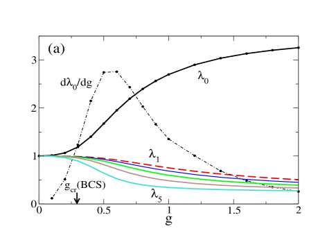
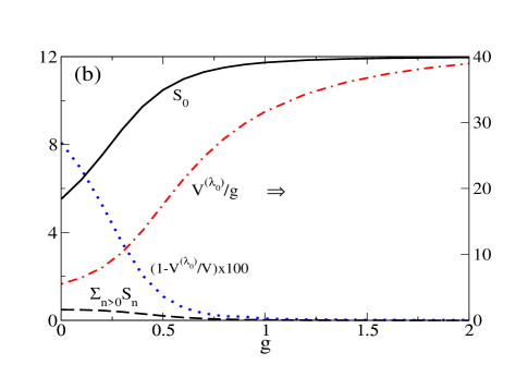
Figure 1: Exact results for a system of 12 particles moving in 12 doubly degenerate levels. (a) The largest 6 eigenvalues of the two-body density matrix as a function of the pairing strength; for the largest eigenvalue $\lambda_{0}$ it is also shown its derivative to the pairing strength. (b) Various quantities (see text) related to the contribution of the largest eigenvalue to the average of the pairing interaction.

For the system described above the eigenvalues of the two-body density matrix can be calculated exactly by solving the Richardson equations richardson . In Fig. 1a are shown, as a function of pairing strength, the largest 6 eigenvalues of the density matrix (18). In the non-interacting limit, i.e. $g=0$, these eigenvalues are equal to 1 and correspond to the 6 occupied levels. When the strength of the pairing interaction is switched on, one eigenvalue becomes greater than 1 while the others smaller than 1. It is also observed that, at variance with the infinite systems, the second largest eigenvalue $\lambda_{1}$ is not too much different from the largest eigenvalue $\lambda_{0}$.

The dependence of $\lambda_{0}$ on the pairing strength indicates how the system evolves from a normal Hartree-Fock (HF)- like state to a paired phase. In order to better visualize the evolution of the largest eigenvalue with $g$, in Fig. 1a we display its derivative with respect to the strength. One can observe that the system evolves quite fast to a paired phase, the fastest variation taking place for $g>g_{cr}$, where $g_{cr}$ is the critical value of the strength in the BCS approximation. It is interesting to notice that $d\lambda_{0}/dg$ is quite similar in shape to the invariant correlation entropy, which is another way of analyzing the evolution of a system toward a paired phase volya .

With the two-body density matrix one can evaluate the expectation value of any two-body operator. Of special interest is the expectation value of the two-body interaction in the ground state of the system

$$V\equiv\langle\Phi_{0}|\hat{V}|\Phi_{0}\rangle=\sum_{ik}V_{ik}\rho_{ik},$$ (26)

which can be written as

$$V=\sum_{n}\lambda_{n}\sum_{ik}V_{ik}f^{(n)}_{i}f^{(n)}_{k}\equiv\sum_{n}V^{(\lambda_{n})}.$$ (27)

In the case of a state independent pairing interaction, when $V_{ik}=g\sqrt{(2j_{i}+1)(2j_{k}+1)}$, one gets

$$V=g\sum_{n}\lambda_{n}(\sum_{i}\sqrt{2j_{i}+1}f^{(n)}_{i})^{2}.$$ (28)

For the system analyzed here all the states have j=1/2 and therefore for each eigenvalue $\lambda_{n}$ the important quantity is $S_{n}=(\sum_{i}f^{(n)}_{i})^{2}$. In Fig. 1b it is shown the quantity $V^{(\lambda_{0})}/g=\lambda_{0}S_{0}$, which represents the contribution of the largest eigenvalue to the average of the pairing interaction in units of the pairing strength, and the quantity $(1-V^{(\lambda_{0})}/V)\times 100$. From the latter one can notice that the main contribution to $V$ comes from the largest eigenvalue, in spite of the fact that the other eigenvalues are also quite large, especially in the weak coupling regime. This is due to the fact that the components $f^{(n)}_{i}$ relative to $\lambda_{n}$ act coherently only for the largest eigenvalue. More precisely, all the components $f^{(0)}_{i}$ turn out to have the same sign, which is not the case for the eigenfunctions corresponding to the other eigenvectors. Due to this fact, the quantity $S_{0}$ is much larger than $S_{n>0}$. This can be seen in Fig. 1b where it is plotted $S_{0}$ and $\sum_{0<n\leq 5}S_{n}$.

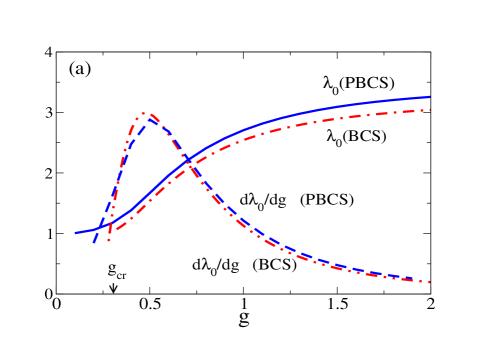
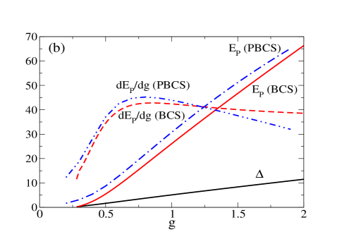
Figure 2: BCS and PBCS results for a system of 12 particles moving in 12 doubly degenerate levels. (a) The largest eigenvalue of the two-body density matrix and its derivative to the pairing strength. (b) The pairing energies and their derivatives to the pairing strength. $\Delta$ is the BCS pairing gap.

In Fig. 2a is shown, for the same system, the largest eigenvalue calculated in the BCS approximation. In BCS there is a phase transition from the normal phase to the BCS pairing phase at $g=g_{cr}$. Then, for $g>g_{cr}$ the largest eigenvalue is increasing rather fast, in a similar manner as for the exact solution. In particular, $d\lambda_{0}/dg$ is reaching the maximum value in the same region of the strength as in the case of the exact solution.

In Fig. 2a are also shown the results obtained in the particle-number projected BCS (PBCS) approximation bayman ; pbcs . Within PBCS the ground state of the system is described by the ansatz

$$|PBCS\rangle=(\Gamma^{+})^{N/2}|0\rangle,$$ (29)

where $\Gamma^{+}=\sum_{i}x_{i}a^{+}_{i}a^{+}_{\bar{i}}$ is the collective Cooper pair. The variational parameters $x_{i}$ are determined from the minimization of the average of the Hamiltonian in the PBCS state, calculated with the method of recurrence relations sandulescu_errea . Since the PBCS is built by applying the same pair operator on $|0\rangle$, the PBCS state is usually called a pair condensate. When the pairing correlations are vanishing, the PBCS state becomes a HF-like state. Comparing Fig. 2a with Fig. 1a one can observe that the PBCS results follow closely the exact results in all the coupling regimes, from weak to strong coupling. One can also notice that, as in the case of the exact solution, the PBCS results evolve smoothly across the region $g=g_{cr}$ where BCS predicts a phase transition.

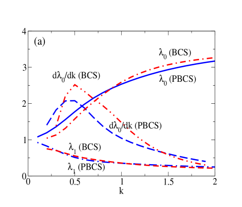
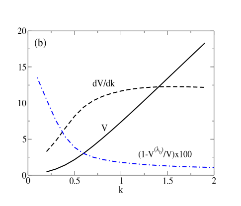
Figure 3: BCS and PBCS results for ¹¹⁰Sn. (a) The largest ( $\lambda_{0}$) and the second largest ( $\lambda_{1}$) eigenvalues of two-body density matrix as a function of the scaling factor $k$. (b) The average of the pairing force, $V$, its derivative to $k$ and the quantity $(1-V^{(\lambda_{0})}/V)\times 100$ calculated in the BCS approximation.

In Fig. 2b are shown the BCS and PBCS results for the pairing energies and their derivatives to the pairing strength. The pairing energy is defined as the average of the pairing interaction from which it is subtracted the self-energy contribution. One observes that the pairing energies have a fast increase in the same region as for the largest eigenvalue, supporting the association of the latter to the evolution towards a paired phase. In Fig. 2d it is also shown the dependence of the BCS pairing gap on the pairing strength. At variance with the largest eigenvalue and the pairing energy, this quantity has a rather constant increase with the pairing strength.

In what follows we discuss the properties of the two-body density matrix taking as example a realistic system, i.e. the nucleus ¹¹⁰Sn. To describe the pairing correlations in this nucleus we use as input for the Hamiltonian (1) the single-particle energies and the two-body pairing matrix elements from Ref. volya . In order to study how the strength of the interaction affects the eigenvalues of two-body density matrix, the pairing matrix elements are scaled by a factor $k$ around the optimal physical value (corresponding to $k$=1). The results for the largest and the second largest eigenvalues provided by BCS and PBCS approximations are displayed in Fig. 3a. The largest eigenvalue has its fastest increase below k=1 and above the region where BCS has a nontrivial solution. As in the picket fence model discussed above, the largest eigenvalue and its derivative provided by PBCS evolve smoothly across the region where the BCS solution sets in. This smooth behaviour of the largest eigenvalue is in keeping with the fact that in finite system there is a gradual change of the structure of the ground state, from a HF-like state to a paired state, in contrast with the sudden phase transition predicted by BCS.

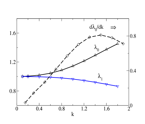
Figure 4: The exact results for the largest and the second largest eigenvalues of two-body density matrix for ²⁴O . The calculations are done with the matrix elements ( $J=0,T=1$) of the USDB interaction which are scaled by the factor $k$.

In Fig. 3b it is shown the average of the pairing force, $V$, and the quantity $(1-V^{(\lambda_{0})}/V)\times 100$. As in the case of Fig. 2b, one can observe that: (i) $V$ and the largest eigenvalue $\lambda_{0}$ have the fastest increase in the same region of the pairing strength; (ii) the largest contribution to $V$ is coming from the largest eigenvalue.

In order to illustrate what happens in systems in which the like-particle pairing correlations are weak, in Fig. 4 are shown the largest two eigenvalues for ²⁴O. The results corresponds to the exact diagonalisation performed for a pairing force extracted from the (J=0,T=1) part of the realistic USDB interaction usd which is scaled by a factor $k$. From Fig. 4 one can observe that at $k=1$ the ratio between the largest and the second largest eigenvalue are much smaller than in the case of ¹¹⁰Sn. In addition, the derivative of the largest eigenvalue indicates that in ²⁴O the transition region to the paired phase is extended beyond $k=1$. Apart from these differences, related to the intensity of pairing correlations, these results shows the same pattern as in the systems analysed above.

IV Eigenvalues of density matrix for proton-neutron pairing interactions

In atomic nuclei one can have pairing correlations not only between like-particles but also between protons and neutrons. These correlations are expected to be the most relevant ones in nuclei with the same number of neutrons and protons since for these nuclei the overlap between the neutron and proton wave functions is maximum. In these nuclei one commonly considers two types of proton-neutron (pn) pairs, i.e. those with angular momentum $J=0$ and isospin $T=1$ and those with $J=1$ and $T=0$ frauendorf ; sagawa . These pairs are called isovector and isoscalar pn pairs, respectively.

The most general spherically symmetric isovector plus isoscalar pairing Hamiltonian reads as

$$H=\sum_{i}\epsilon_{i}N_{i} +\sum_{i,k}V^{01}(i,k)[\mathcal{A}^{+01}(i,i)\mathcal{\widetilde{A}}^{01}(k,k)]^{(0,0)}$$ (30)

$$+\sum_{i\leq i^{\prime},k\leq k^{\prime}}V^{10}(ii^{\prime};kk^{\prime})[\mathcal{A}^{+10}(i,i^{\prime})\mathcal{\widetilde{A}}^{10}(k,k^{\prime})]^{(0,0)}$$

and it refers to a system of protons and neutrons distributed over a set of orbitals $i=\{n_{i},l_{i},j_{i}\}$, where the standard notation for spherical single-particle states has been adopted. In this expression, $\epsilon_{i}$ and $N_{i}$ are the energy and the total particle number operator relative to the orbital $i$, respectively. Pair creation operators are defined as

$$\mathcal{A}^{+JT}_{J_{z},T_{z}}(i,i^{\prime})=\frac{1}{\sqrt{(1+\delta(i,i^{\prime}))}}[a^{+}_{i}a^{+}_{i^{\prime}}]^{J,T}_{J_{z},T_{z}},$$ (31)

with $J,T$ being the angular momentum and isospin of the pair and $J_{z},T_{z}$ their relative projections. For the pair annihilation operators we have adopted the standard definition ${\widetilde{A}}^{JT}_{J_{z},T_{z}}(i,i^{\prime})=(-1)^{J-J_{z}+T-T_{z}}{A}^{JT}_{-J_{z},-T_{z}}(i,i^{\prime})$. The second and the third terms of Eq. (30) describe the isovector and the isoscalar pairing interactions, respectively. The Coulomb interaction between the protons has been neglected.

The Hamiltonian (30) is commonly used to investigate in $N=Z$ nuclei the presence of correlations of superfluid type associated with isovector and isoscalar proton-neutron pairs (goodman_adv ; goodman_prc ; gerzelis . The issue we study here is whether for these pairs the density matrix has properties similar to those observed for the like-particle pairing. In order to perform this study we construct the two-body density matrix in term of pairs of arbitrary $(J,T)$ defined by

$$\rho^{(2)}_{JT}(ii^{\prime},kk^{\prime})=\sqrt{2J+1}\sqrt{2T+1}\langle\Phi^{(N)}_{0}|[\mathcal{A}^{+JT}(i,i^{\prime})\mathcal{\widetilde{A}}^{+JT}(k,k^{\prime})]^{J=0,T=0}|\Phi^{(N)}_{0}\rangle$$ (32)

with $i\leq i^{\prime}$ and $k\leq k^{\prime}$. Of interest for this study are the density matrices for $(J=0,T=1)$ and $(J=1,T=0)$.

As an illustration, we present in the following the results for the $N=Z$ nucleus ³²S. As input for the Hamiltonian (30) we have used the single-particle energies and the matrix elements for $(J=0,T=1)$ and $(J=1,T=0)$ extracted from the interaction USDB usd . The density matrix has been calculated in correspondence with the exact eigenstates of the Hamiltonian (30).

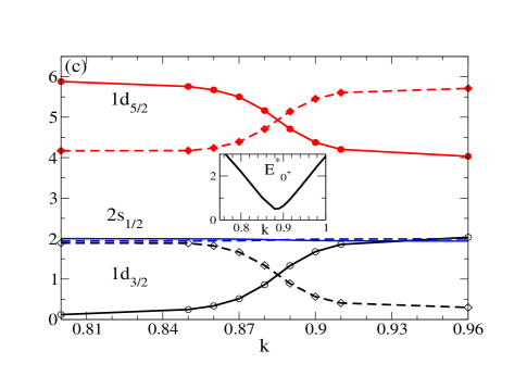
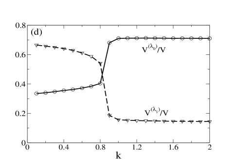
Figure 5: (a) The largest and the second largest eigenvalues of the two-body density matrix for the isovector pairing interaction scaled by the factor $k$. (b) The same as in (a) but for the isoscalar pairing interaction. (c) The occupancy of the single-particle states of the $sd$ valence shell in the case of a pure $T=0,J=1$ force. The insets in (b) and (c) show the excitation energy of the first excited state $0^{+}$. (d) The ratios $V^{(\lambda_{0})}/V$ and $V^{(\lambda_{1})}/V$ for the isoscalar interaction. All results corresponds to ³²S.

We begin by analysing the eigenvalues of the two-body density matrix in the case of an isovector interaction only. The strength of the interaction has been varied by multiplying all the $(J=0,T=1)$ USDB matrix elements by a scaling factor $k$. The dependence of the largest two eigenvalues of the density matrix on the scaling factor $k$ is shown in Fig. 5a. In the density matrix (32) are added together the contribution of the proton-neutron, neutron-neutron and proton-proton pairs which, due to the isospin invariance of the interaction, are equal to each other. As a consequence, one observes that in the non-interacting limit the eigenvalues of the density matrix for $(J=0,T=1)$ are equal to 3. Fig. 5a shows that, with increasing the interaction, the two largest eigenvalues behave as in the case of the nucleus ²⁴O (Fig. 4), which has the same number of neutrons as ³²S. Thus, as expected from the isospin invariance, the properties of the density matrix for the isovector proton-neutron pairing are similar to those observed in the previous section in the case of the neutron-neutron pairing.

As a next step we analyse the results for the isoscalar interaction only, i.e. when from the USDB interaction we retain only the matrix elements with $(J=1,T=0)$. The results for the largest two eigenvalues of the density matrix, as a function of the scaling factor $k$, are shown in Fig. 5b. As in the case of isovector pairing one can see that in the non-interacting case the eigenvalues are equal to 3. This is due to the fact that in the density matrix for $(J=1,T=0)$ we are summing the three equal contributions of the pairs with $J_{z}=\{-1,0,1\}$. From Fig. 5b one can observe that up to $k\approx 0.8$ the largest two eigenvalues change little compared to the non-interacting value. Then, between $k\approx 0.8$ and $k\approx 1.0$ the largest eigenvalue increases suddenly while the second largest decreases. Afterwards, for $k>1$, the two eigenvalues change slowly with increasing the interaction strength. Interestingly, in the region where the eigenvalues have a sudden change there is a fast decrease of the energy of the first excited $0^{+}$ state. As seen in the inset of Fig. 5b, for $k\approx 0.88$ the energy of the excited state comes very close to the ground state energy, indicating a level crossing. This crossing is also reflected in the interchange between the occupancies of the spin-orbit partners $1d_{5/2}$ and $1d_{3/2}$ which is illustrated in Fig. 5c.

In Fig. 5d we show the quantities $V^{(\lambda_{0})}$ and $V^{(\lambda_{1})}$ relative to $V$. We can see that the contribution of the largest eigenvalue to the average interaction is much smaller than for the like-particle pairing. This is due to the fact that the amplitudes $f^{(0)}_{i}$ have mixed signs, so they do not add coherently in $V^{(\lambda_{0})}$. This is also the case for the other eigenvectors. Surprisingly, below $k\approx 0.8$ the contribution of the largest eigenvalue is in fact much smaller than the contribution of the second largest eigenvalue. Since in this region the two eigenvalues are very close to each other, this means that the contribution arising from the $f^{(1)}_{i}$’s is larger than that from the $f^{(0)}_{i}$’s. In Fig. 5d one can also notice that above $k\approx 0.8$ the two ratios depends very weakly on the pairing strength. This is another indication that the sudden increase of the largest eigenvalue of the density matrix with the strength of the isoscalar interaction is not related to a transition towards a paired phase.

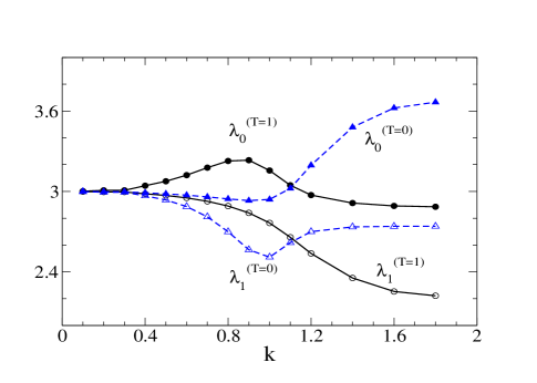
Figure 6: The largest two eigenvalues of the two-body density matrix for T=0 and T=1 pairs obtained with the isovector plus the isoscalar pairing interactions scaled by the factor $k$. The results correspond to ³²S.

In what follows we analyse the eigenvalues of the density matrix when the Hamiltonian (30) contains both the isovector and the isoscalar components. As in the calculations presented above, for the two interactions we have considered the matrix elements with $(J=0,T=1)$ and $(J=1,T=0)$ extracted from the USDB interaction. Thus the relative strength of the interaction in the two channels is fixed by the realistic USDB force. The calculations for the density matrix are done by scaling both interactions with the same factor $k$. The results for the largest and the second largest eigenvalues of the density matrix, corresponding to the exact ground state, are shown in Fig. 6. One observes that for $J=0$ the largest eigenvalue slowly increases up to around $k=0.8$ and then, for $k>0.9$, it decreases towards the non-interacting value. This decrease is not seen in the case of pure isovector interaction shown in Fig. 5a, which means that this is an effect caused by the isoscalar pairing interaction . On the other hand, as seen in Fig. 6, the largest eigenvalue for $J=1$ has a shape rather similar to the case of the pure isoscalar interaction. At a closer inspection one can notice, however, that the presence of the isovector force has some effects on the behavior of the largest eigenvalue with $J=1$. One can indeed see that this slowly decreases for $k<1$, which is not so for the pure isoscalar force. As it will be shown below, this decrease becomes significantly large in the presence of the other multipoles of the two-body interaction.

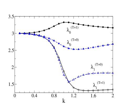
Figure 7: The largest two eigenvalues of the two-body density matrix for T=0 and T=1 pairs obtained with the USD interaction scaled by the factor $k$. The results corresponds to the exact ground state of ³²S.

Finally we analyse the eigenvalues of the two-body density matrix for the $J=0$ and $J=1$ pairs in the case of the full shell model Hamiltonian

$$H=\sum_{i}\epsilon_{i}N_{i}+\sum_{i\leq i^{\prime},k\leq k^{\prime},J,T}V^{JT}(ii^{\prime};kk^{\prime})\sqrt{2J+1}\sqrt{2T+1}[\mathcal{A}^{+JT}(i,i^{\prime})\mathcal{\widetilde{A}}^{JT}(k,k^{\prime})]^{(0,0)},$$ (33)

where the sum over $J,T$ includes all possible pairs. The question of interest here is how the two-body density matrices for the ($J=0,T=1)$ and $(J=1,T=0)$ pairs are affected when, in addition to the interaction in these two channels, one considers also all the other components of the shell model interaction. In order to study this issue, we have evaluated the two-body density matrices using the exact wave functions of the shell model (SM) Hamiltonian (33). In the SM calculations, performed with the code BIGSTICK bigstick , we have used the USDB interaction scaled by a factor $k$. The results for the largest and the second largest eigenvalues of the density matrix in the channels $(J=0,T=1)$ and $(J=1,T=0)$ are shown in Fig. 7. For $J=0$ the behavior of the largest eigenvalue is rather similar to the one shown in Fig. 6, with the difference that for $k>1$ the decrease is slower. The situation is completely different for the $J=1$ pairing. In this case the largest eigenvalue decreases very fast up to around $k=1.1$ and then it only slightly increases. This shows that the peculiar fast increase of the largest eigenvalue observed in the case of the isoscalar and the isoscalar-isovector pairing interactions is washed out by the other components of the SM interaction.

V Summary and Conclusions

In this paper we have presented a detailed study of the two-body density matrix corresponding to the interactions commonly employed to describe pairing correlations in atomic nuclei. After a general introduction on the properties of the density matrix we have first analysed the eigenvalues of the two-body density matrix for various like-particle pairing interactions. In all the cases investigated we have observed that the behaviour of the largest eigenvalue of the density matrix provides a clear indication of the transition from a normal to a paired phase. Indeed, at variance with the remaining eigenvalues, the largest eigenvalue has a fast and continuous increase in the region of the pairing strength where a standard BCS approach predicts strong pairing correlations. However, differently from what happens in infinite systems, the largest eigenvalue is not found too much different in magnitude as compared to the other eigenvalues, especially in the weak coupling regime. In spite of that, the largest eigenvalue is responsible for the dominant contribution in the expectation value of the pairing interaction, as in the case of infinite systems. This is due to the fact that the eigenfunction corresponding to the largest eigenvalue has a coherent structure, i.e. all its components have the same sign. In the like-particle pairing case we have also noticed a close agreement between exact and PBCS results for the largest eigenvalue of the density matrix. This finding is consistent with the good agreement found for the correlation energies in previous studies. It is worth mentioning that a close agreement between PBCS and the exact results can be obtained only when the pairing acts in a limited window around the Fermi level of the order of the pairing gap sandulescu_bertsch .

In the second part of the paper we have studied the properties of the density matrix for the isoscalar ($J=0$, $T=1$) and the isovector ($J=1$, $T=0$) proton-neutron pairing interactions. For this study we have considered as example the nucleus ³²S. The results for the isovector interaction are rather similar to those for the like-particle pairing. Very different results have been obtained instead for the isoscalar interaction. In this case the largest $J=1$ eigenvalue has a sudden increase when the strength of the interaction is scaled around the physical value. A detailed analysis shows, however, that this sudden increase of the largest eigenvalue is in fact related to the crossing between the ground state and the first excited $0^{+}$ state and not to a transition towards a paired phase.

We have also analysed the eigenvalues of the density matrix when the isovector and the isoscalar pairing interactions are acting together. The results for this case are not significantly different from those corresponding to the pure pairing forces mentioned above, except for the decrease of the largest $J=0$ eigenvalue for large values of the pairing strength.

Finally, in the last part of the paper we have studied the properties of the two-body density matrix for a general interaction. As example we have taken the standard shell-model two-body interaction which is commonly applied to describe the nucleus ³²S. We found that the largest $J=1$ eigenvalue is decreasing very fast with the increase of the interaction strength, arriving to values below those at the non-interacting regime for strengths around the physical value. This is an indication that no long-range two-body correlations can be associated with $J=1$ pairs in the case of the general interaction .

In the present study we have focused on the two-body correlations associate to proton-neutron pairing interactions. However, in the N=Z systems these interactions generate also 4-body correlations soloviev ; flower ; bremond ; eichler ; dobes_pittel ; chapman ; qcm_nez ; qcm_plb ; qm_t1 . In particular, as shown recently, the isovector plus isoscalar Hamiltonian (30) can be treated accurately in terms of alpha-like quartets built by two protons and two neutrons coupled to total isospin $T=0$, rather than in terms of Cooper pairs qcm_t0t1 . It has also been shown that $T=0$ alpha-like quartets are the main building blocks for systems governed by the general shell model Hamiltonian (33) hasegawa1 ; qm_prl ; qcm_epja . These studies clearly show that 4-body correlations play a key role in the N=Z nuclei. How these correlations are reflecting in the 4-body density matrix is an interesting issue which will be addressed in a future publication.

Acknowledgements N. S. would like to thank for the hospitality of Royal Institute of Technology, Stockholm, where this paper was mainly written. This work was supported by the Romanian National Authority for Scientific Research, CNCS UEFISCDI, Project Number PN-II-ID-PCE-2011-3-0596.

References

- (1) O. Penrose, Phil. Mag. 42, 1373 (1951).
- (2) O. Penrose and L. Onsager, Phys. Rev. 104, 576 (1956).
- (3) C. N. Yang, Rev. Mod. Phys. 34, 694 (1962).
- (4) J. Bardeen, L. N. Cooper, and J. R. Schrieffer, Phys. Rev. 108, 1175(1957).
- (5) A. Bohr and B. Mottelson, Nuclear Structure (World Scientific, 1998).
- (6) R. W. Richardson and N. Sherman, Nucl. Phys. 52, 221 (1964).
- (7) B. F. Bayman, Nucl. Phys. 15, 33 (1960).
- (8) K. Dietrich, H. J. Mang, and J. H. Pradal, Phys. Rev. 135, B22 (1964).
- (9) K. Langanke, D. J. Dean, P. B. Radha, S. E. Koonin, Nucl. Phys. A 602, 244 (1996).
- (10) S. Frauendorf and A. O. Macchiavelli, Prog. Part. Nucl. Phys. 78, 24 (2014).
- (11) H. Sagawa, C. L. Bai, and G. Colo, Phys. Scripta 91, 083011 (2016).
- (12) A. Leggett, Quantum Liquids (Oxford University Press, 2006).
- (13) V.L. Ginzburg and L.D. Landau, Zh. Eksp. Teor. Fiz. 20, 1064 (1950).
- (14) N. Sandulescu, P. Schuck, X. Vinas, Phys. Rev. C 71, 054303 (2005).
- (15) N. Pillet, N. Sandulescu, P. Schuck, Phys. Rev. C 76, 024310 (2007).
- (16) M. Schechter, Y. Imry, Y. Levinson, and J. von Delft, Phys. Rev. B 63, 214518 (2001).
- (17) J. von Delft and D. C. Ralph, Phys. Rep. 345, 61 (2001).
- (18) A. Volya, V. Zelevinsky, Phys. Lett. B 574, 27 (2003).
- (19) N. Sandulescu, B. Errea, J. Dukelsky, Phys. Rev. C 80, 044335 (2009).
- (20) B.A. Brown and W.A. Richter, Phys. Rev. C 74, 034315 (2006).
- (21) A. L. Goodman, Adv. Nucl. Phys. 11, 263 (1979).
- (22) A.L. Goodman, Phys. Rev. C 60, 014311 (1999).
- (23) A. Gezerlis, G.F. Bertsch, Y.L. Luo, Phys. Rev. Lett. 106, 252502 (2011).
- (24) C. W. Johnson,W. E. Ormand, K. S. McElvain, and H. Z. Shan, arXiv: 1801.08432.
- (25) N. Sandulescu, G. Bertsch, Phys. Rev. C 78, 064318 (2008).
- (26) V.G. Soloviev, Nucl. Phys. 18, 161 (1960).
- (27) B. H. Flowers and M. Vujicic, Nucl. Phys. 49, 586 (1963).
- (28) B. Bremond, J.G. Valatin, Nucl. Phys. 41, 640 (1963).
- (29) J. Eichler and M. Yamamura, Nucl. Phys. A 182, 33 (1972).
- (30) J. Dobes and S. Pittel, Phys. Rev. C 57, 688 (1998).
- (31) R.R. Chasman, Phys. Lett. B 577, 47 (2003).
- (32) N. Sandulescu, D. Negrea, J. Dukelsky, C. W. Johnson, Phys. Rev. C 85, 061303(R) (2012).
- (33) N. Sandulescu, D. Negrea, and D. Gambacurta, Phys. Lett. B 751, 348 (2015).
- (34) M. Sambataro and N. Sandulescu, Phys. Rev. C 88, 061303(R) (2013).
- (35) M. Sambataro, N. Sandulescu, C.W. Johnson, Phys. Lett. B740, 137 (2015).
- (36) M. Hasegawa, S. Tazaki, and R. Okamoto, Nucl. Phys. A 592, 45 (1995).
- (37) M. Sambataro and N. Sandulescu, Phys. Rev. Lett. 115, 112501 (2015).
- (38) M. Sambataro and N. Sandulescu, Eur. Phys. J. A 53, 47 (2017).