Relativistic and non-Gaussianity contributions to the one-loop power spectrum

Abstract

We compute the one-loop density power spectrum including Newtonian and relativistic contributions, as well as the primordial non-Gaussianity contributions from $f_{\rm NL}$ and $g_{\rm NL}$ in the local configuration. To this end we take solutions to the Einstein equations in the long-wavelength approximation and provide expressions for the matter density perturbation at second and third order. These solutions have shown to be complementary to the usual Newtonian cosmological perturbations. We confirm a sub-dominant effect from pure relativistic terms, manifested at scales dominated by cosmic variance, but find that a sizable effect of order one comes from $g_{\rm NL}$ values allowed by Planck-2018 constraints, manifested at scales probed by forthcoming galaxy surveys like DESI and Euclid. As a complement, we present the matter bispectrum at the tree-level including the mentioned contributions.

1 Introduction

The upcoming Stage IV experiments like DESI [1] and Euclid [2] aim to map the large-scale structure (LSS) of the Universe at high-precision. For many years the Newtonian standard perturbation theory (SPT) [3, 4, 5] was sufficient to study the evolution of the matter content of the Universe. However, the Newtonian description of the Universe is only adequate for scales well inside the horizon and non-relativistic matter. The scales explored by the future surveys make a relativistic description of the dynamics of the Universe essential. The analysis of the new data gathered by new experiments requires the use of sophisticated statistical tools. The power spectrum and bispectrum density fluctuations in the matter are key quantities to study the formation and composition of the LSS.

Recent analytic and numerical work began to include relativistic effects into the density power spectrum and bispectrum. In particular: relativistic corrections to the power spectrum [6, 7], one-loop relativistic corrections for the power spectrum and bispectrum on intermediate scales using the weak field approximation [8], galactic non-linear bias from gravitational non-linearity [9, 10, 11, 12, 13], and N-body simulations using General Relativity (GR) [14, 15, 16].

In order to account for relativistic contributions to observables, a complementary strategy is to integrate the signals produced by galaxies along the line of sight to determine the distance-redshift relation. The resulting distortions of redshift-space due to structure have been reported in terms of the number counts of galaxy clustering at linear order [17, 18, 19, 20, 21], and at second order [22, 23, 24, 25, 26, 27, 28, 29, 30]. Moreover, the observed bispectrum receives contributions from this relation as shown recently in [24, 31, 32, 33, 34, 35, 36].

One of the quantities that the community aims to constrain with the data released by the forthcoming surveys, is the primordial non-Gaussianity (PNG) generated during inflation. The inflationary epoch is crucial for early structure formation and the later evolution of the LSS [37, 38, 39], which makes constraining the PNG such an exciting prospect (see e.g. Ref. [40] for a review), as this offers the possibility to probe different inflationary scenarios (see also Refs. [41, 42] for prospects of detection). The effects of non-Gaussianity on the power spectrum have been previously studied in Refs. [43, 44], although not from a relativistic point of view. In Ref. [9] the authors include relativistic corrections to the galaxy power spectrum including primordial non-Gaussianities from $f_{\rm NL}$ in the local configuration. In Ref. [45] the galaxy bispectrum in redshift space, including PNG, is calculated. In Refs. [46, 47] the effective non-Gaussianity from relativistic corrections to the bispectrum of galaxies is determined.

The goal of this paper is to include contributions from the scalar sector of the full relativistic theory at second and third order, as well as the primordial non-Gaussianity at the same orders (which can be easily included as an additional term in the chosen gauge; the synchronous-comoving gauge), and analyse their effects on the power spectrum at one-loop and the tree-level bispectrum.

The paper is organised as follows: in section 2 we review work previously done and present the evolution equations for the density contrast in synchronous-comoving gauge. We present its solutions up to third order using the gradient expansion. These solutions assume an Einstein-de Sitter Universe and are necessary for the computation of the one-loop power spectrum. In section 3, we present the Newtonian and relativistic solutions for the density contrast in Fourier space. Section 4 is dedicated to the one-loop power spectrum, which is our main result. We provide complete analytical expressions for the one-loop power spectrum, along with numerical integrations, including the contributions to the one-loop power spectrum for the allowed values of $f_{\rm NL}$ and $g_{\rm NL}$ reported by Planck [48]. For completeness, in section 5 we present the tree-level bispectrum, along with numerical solutions. Finally, in section 6 we discuss our results in light of the forthcoming galaxy surveys.

Throughout this paper we use the conformal time $\eta$, and denote derivatives with respect to $\eta$ with a prime. Greek indices $\mu$, $\nu$, range from 0 to 3, lower case Latin indices, $i$, $j$, and $k$, have the range 1, 2, 3.

2 Evolution equations and relativistic density contrast solutions

In this section we present the evolution equations for the density contrast in synchronous-comoving gauge, based on work previously done in Refs. [49, 50, 51]. The choice of this gauge provides a Lagrangian frame in GR, which is also suitable for defining local Lagrangian galaxy bias up to second order [10]. Our starting point is the general line element,

$$ds^{2}=a^{2}(\eta)[-(1+2\phi)d\eta^{2}+2\omega_{,i}d\eta dx^{i}+\gamma_{ij}dx^{i}dx^{j}],$$ (2.1)

where $a$ is the scale factor, $\eta$ is the conformal time, $\phi$ and $\omega$ are scalar metric perturbations and $\gamma_{ij}$ is the spatial metric. As we will work in the synchronous comoving gauge, we set $\phi=\omega_{,i}=0$.

As the matter content we consider an irrotational, pressureless fluid. Observers are comoving with the fluid, and as a consequence the four-velocity in the synchronous comoving gauge is $u_{\mu}=(-a,0,0,0)$.

For the following fluid description, we define the deformation tensor,

$${\vartheta}_{\nu}^{\mu}\equiv a{u^{\mu}}_{;\nu}-\mathcal{H}\delta_{\nu}^{\mu},$$ (2.2)

where $\mathcal{H}=a^{\prime}/a$ is the conformal Hubble scalar, the semicolon denotes covariant derivative and the isotropic background expansion was removed. In the chosen gauge, the deformation tensor has only spatial components and is proportional to the extrinsic curvature $K_{j}^{i}$ of the conformal spatial metric $\gamma_{ij}$,

$$\vartheta_{j}^{i}=-K_{j}^{i},$$ (2.3)

where $K_{j}^{i}$ is given by

$$K_{j}^{i}\equiv-\frac{1}{2}\gamma^{ik}\gamma_{kj}^{\prime}.$$ (2.4)

The density field $\rho$ is defined as

$$\rho(\mathbf{x},\eta)=\bar{\rho}(\eta)+\delta\rho(\mathbf{x},\eta)=\bar{\rho}(\eta)(1+\delta(\mathbf{x},\eta)),$$ (2.5)

where $\bar{\rho}(\eta)$ is the density in the background, $\delta\rho(\mathbf{x},\eta)$ is a small perturbation and $\delta(\mathbf{x},\eta)$ is the density contrast. The evolution of the density contrast $\delta(\mathbf{x},\eta)$ is given by the continuity equation

$$\delta^{\prime}+(1+\delta)\vartheta=0,$$ (2.6)

where $\vartheta=\vartheta_{\alpha}^{\alpha}$ is the trace of $\vartheta_{\nu}^{\mu}$.

The evolution for $\vartheta$ is given by the Raychaudhuri equation (more details of the derivation can be found in Refs. [51, 52])

$$\vartheta^{\prime}+\mathcal{H}\vartheta+\vartheta_{j}^{i}\vartheta_{i}^{j}+4\pi Ga^{2}\bar{\rho}\delta=0.$$ (2.7)

The energy constraint is given by

$$\vartheta^{2}-\vartheta_{j}^{i}\vartheta_{i}^{j}+4\mathcal{H}\vartheta+{}^{3}R=16\pi Ga^{2}\bar{\rho}\delta,$$ (2.8)

where ${}^{3}R$ is the spatial Ricci scalar of the spatial metric $\gamma_{ij}$. In the following subsections we use two approaches to find solutions to the evolution equations.

2.1 Cosmological perturbation theory

In order to show how cosmological perturbation theory is used to find the evolution of the density contrast, we present in this section the solutions to first order. The line element (2.2) is equivalent to a spatially flat FLRW background with a perturbed spatial metric (in synchronous-comoving gauge), and hence we can expand $\gamma_{ij}$ as in terms of the scalar metric potentials $\psi$ and $\chi$ as

$$\gamma_{ij} =\delta_{ij}+\gamma_{ij}^{(1)}+\frac{1}{2}\gamma_{ij}^{(2)}+...$$

$$=(1-2\psi^{(1)}-\psi^{(2)})\delta_{ij}+\chi_{ij}^{(1)}+\frac{1}{2}\chi_{ij}^{(2)}+...$$ (2.9)

where

$$\chi_{ij}=\left(\partial_{i}\partial_{j}-\frac{1}{3}\delta_{ij}\nabla^{2}\right)\chi.$$ (2.10)

The density contrast is decomposed as

$$\delta=\delta^{(1)}+\frac{1}{2}\delta^{(2)}+\frac{1}{6}\delta^{(3)}+...$$ (2.11)

For the case of the first order solutions for the density contrast, we combine the first order of the continuity equation (2.6) and the Raychaudhuri equation (2.7) at first order, to obtain the first order density contrast evolution equation

$$\delta^{(1)^{\prime\prime}}+\mathcal{H}\delta^{(1)^{\prime}}-\frac{3}{2}\mathcal{H}^{2}\Omega_{m}\delta^{(1)}=0.$$ (2.12)

From the first order energy constraint equation (2.8), combined with the first order continuity equation (2.6) we obtain

$$4\mathcal{H}\delta^{(1)^{\prime}}+6\mathcal{H}^{2}\Omega_{m}\delta^{(1)}-{}^{3}R^{(1)}=0,$$ (2.13)

combining the time derivative of the Eq.(2.13) and using the first order of Eqs. (2.6) and (2.7) we find an equation for $R^{(1)}$ given by

$${}^{3}R^{(1)^{\prime}}=0.$$ (2.14)

The general solution for a second order differential equation, will be composed of a linear combination of a growing mode and a decaying mode

$$\delta^{(1)}(\eta,\mathbf{x})=C_{+}(\mathbf{x})D_{+}(\eta)+C_{-}(\mathbf{x})D_{-}(\eta).$$ (2.15)

Since we choose to work in an Einstein-de Sitter universe, the decaying mode solution is negligible and from now on we take a solution of the form

$$\delta^{(1)}(\eta,\mathbf{x})=C(\mathbf{x})D_{+}(\eta),$$ (2.16)

where $C(\mathbf{x})$ will be given by [51]

$$C(\mathbf{x})=\frac{{}^{3}R^{(1)}}{10\mathcal{H}_{IN}^{2}D_{+IN}},$$ (2.17)

$D_{+}$ is the growth factor, and the subscript “$IN$” denotes a time early in the matter dominated era.

At first order in perturbative, for an unspecified gauge, the spatial Ricci scalar, is

$${}^{3}R^{(1)}=4\nabla^{2}\left(\psi^{(1)}+\frac{1}{6}\nabla^{2}\chi^{(1)}\right).$$ (2.18)

From Eq. (2.18) in the comoving gauge, we can identify the comoving curvature perturbation, $\mathcal{R}_{c}$, [53, 54]

$$\mathcal{R}_{c}=\psi^{(1)}_{c}+\frac{1}{6}\nabla^{2}\chi^{(1)}_{c}.$$ (2.19)

The comoving curvature perturbation is related with the curvature perturbation on the uniform-density gauge as (see for example Ref. [53])

$$\zeta^{(1)}\equiv-\psi^{(1)}-\frac{1}{6}\nabla^{2}\chi^{(1)}-\frac{\mathcal{H}}{\rho^{\prime}}\delta\rho^{(1)}=-\mathcal{R}_{c}+\frac{1}{3}\delta^{(1)},$$ (2.20)

and at early times and large scales $\zeta^{(1)}$ and $\mathcal{R}_{c}$ are approximately equal:

$$\zeta^{(1)}\simeq-\mathcal{R}_{c}.$$ (2.21)

Substituting Eq. (2.21) into Eq. (2.18), we write the first order solution for the density contrast as

$$\delta^{(1)}=\frac{D_{+}(\eta)}{10\mathcal{H}^{2}_{IN}D_{+IN}}\left(-4\nabla^{2}\zeta^{(1)}\right),$$ (2.22)

where the growth factor in Einstein-de Sitter is

$$D_{+}=\frac{D_{+IN}\mathcal{H}_{IN}^{2}}{\mathcal{H}^{2}},$$ (2.23)

with $D_{+IN}=1$ and $\mathcal{H}_{IN}=\mathcal{H}_{0}$, where $\mathcal{H}_{0}$ is the conformal Hubble parameter at present time. These choices are made to recover the standard Newtonian solutions.

2.2 Gradient expansion approach

In section 2.1 we presented the first order equations and solutions for the density contrast using cosmological perturbation theory, in this section we present the solutions for the second and third order equations using a different approach, the gradient expansion, that leads to the same equations and solutions obtained using the perturbative treatment. Instead of using the expansion Eq. (2.1), we can also write the spatial metric as [55, 56]

$$g_{ij}=a^{2}\gamma_{ij}=a^{2}e^{2\zeta}\check{\gamma}_{ij},$$ (2.24)

where $\zeta$ is the curvature perturbation on uniform density hypersurfaces.

The initial conditions for perturbations are set in the inflationary epoch. After this period, the curvature perturbation $\zeta$ is almost scale-invariant and remains constant (see for example Ref. [57]). As a consequence is it possible to consider small initial inhomogeneities on large scales, allowing for a gradient expansion [58, 59, 60, 61, 62]. In this long-wavelength approximation the spatial gradients are small compared to time derivatives. Using this approximation we find

$$\delta\sim\vartheta\sim{}^{3}R\sim\nabla^{2},$$ (2.25)

and using this approximation with the continuity (2.6) and energy constraint equations (2.8), lead us back to the Eq. (2.13).

On large scales, and only considering scalars, the conformal metric can be approximated as $\check{\gamma}_{ij}\simeq\delta_{ij}$. As a consequence of this simplified spatial metric, the Ricci scalar $R$ is a nonlinear function of the curvature perturbation $\zeta$ only, taking the form [49, 50, 63]

$${}^{3}R=-4\nabla^{2}\zeta+\sum_{m=0}^{\infty}\frac{\left(-2\right)^{m+1}}{(m+1)!}\left[(m+1)(\nabla\zeta)^{2}-4\zeta\nabla^{2}\zeta\right]\zeta^{m}.$$ (2.26)

This expansion for $R$ will allow us to obtain solutions for the density contrast to higher orders. In this paper we are interested in solutions up to third order. The third order corrections are obtained after expanding $R$ up to $m=1$ and are given by

$${}^{3}R=-4\nabla^{2}\zeta+(-2)[(\nabla\zeta)^{2}-4\zeta\nabla^{2}\zeta]+2[2(\nabla\zeta)^{2}-4\zeta\nabla^{2}\zeta]\zeta.$$ (2.27)

The curvature perturbation can be expanded in terms of a Gaussian random field $\zeta^{(1)}$ as

$$\zeta=\zeta^{(1)}+\frac{3}{5}f_{\rm NL}\zeta^{(1)2}+\frac{9}{25}g_{\rm NL}\zeta^{(1)3},$$ (2.28)

where $f_{\rm NL}$ and $g_{\rm NL}$ are the non-Gaussian parameters at first and second order respectively. After substituting Eq. (2.28) into Eq. (2.27), we get an expression for the Ricci scalar, that will allow us to find the density contrast solutions

$${}^{3}R\simeq-4\nabla^{2}\zeta^{(1)} +\left(\nabla\zeta^{(1)}\right)^{2}\left[-2-\frac{24}{5}f_{\rm NL}\right]+\zeta^{(1)}\nabla^{2}\zeta\left[-\frac{24}{5}f_{\rm NL}+8\right]$$

$$+\zeta^{(1)}\left(\nabla\zeta^{(1)}\right)^{2}\left[-\frac{216}{25}g_{\rm NL}+\frac{24}{5}f_{\rm NL}+4\right]$$ (2.29)

$$+\zeta^{(1)2}\nabla^{2}\zeta^{(1)}\left[-\frac{108}{25}g_{\rm NL}+\frac{72}{5}f_{\rm NL}-8\right]+\mathcal{O}(\zeta^{(1)4}).$$

From Eq. (2.2) it is straightforward to see that solutions to first order in the gradient expansion agree with the ones produced using the perturbation theory treatment.

In a similar way to the first order, using the continuity equation (2.6), along with the energy constraint equation (2.8), the second order evolution equation of $\delta$ will be given by

$$4\mathcal{H}\delta^{(2)^{\prime}}+6\mathcal{H}^{2}\Omega_{m}\delta^{(2)}-{}^{3}R^{(2)}=2\vartheta^{(1)2}-2\vartheta^{(1)i}_{j}\vartheta_{i}^{(1)j}-8\mathcal{H}\delta^{(1)}\vartheta^{(1)},$$ (2.30)

using

$${}^{3}R^{(2)^{\prime}}=-4\vartheta^{(1)i}_{j}R_{i}^{(1)j}.$$ (2.31)

As shown in the Ref. [51], the solution for these equations is composed of an homogeneous and a particular solution (labelled with subscripts “$h$” and “$p$” respectively) of the form

$$\delta^{(2)}=\delta_{h}^{(2)}+\delta_{p}^{(2)},\quad{}^{3}R^{(2)}={}^{3}R_{h}^{(2)}+{}^{3}R_{p}^{(2)},$$ (2.32)

where the particular solution recovers the Newtonian density contrast obtained within the Newtonian standard perturbation theory formalism and the homogeneous solution corresponds to the relativistic contributions to the density contrast also presented in Ref.[51].

Thus, using the expansion for the Ricci scalar given in Eq. (2.2) up to second order ($m=0$), the homogeneous solution for the second order of the density contrast is

$$\frac{1}{2}\delta^{(2)}=\frac{D_{+}(\eta)}{10\mathcal{H}^{2}_{IN}D_{+IN}}\frac{24}{5}\Bigg{[}-(\nabla\zeta^{(1)})^{2}\bigg{(}\frac{5}{12}+f_{\rm NL}\bigg{)}+\zeta^{(2)}\nabla^{2}\zeta^{(1)}\bigg{(}\frac{5}{3}-f_{\rm NL}\bigg{)}\Bigg{]},$$ (2.33)

in analogous way the homogeneous third order solution for the density contrast is

$$\frac{1}{6}\delta^{(3)}=\frac{D_{+}(\eta)}{10\mathcal{H}^{2}_{IN}D_{+IN}}\frac{108}{25}\Bigg{[} 2\zeta^{(1)}(\nabla\zeta^{(1)})^{2}\bigg{(}-g_{\rm NL}+\frac{5}{9}f_{\rm NL}+\frac{25}{54}\bigg{)}$$

$$+ \zeta^{(1)2}\nabla^{2}\zeta^{(1)}\bigg{(}-g_{\rm NL}+\frac{10}{3}f_{\rm NL}-\frac{50}{27}\bigg{)}\Bigg{]},$$ (2.34)

which slightly differs from the expression provided in Ref. [49]. We are interested in the new effects to the one-loop power spectrum due to Newtonian and relativistic contributions focusing on the derivation of the relativistic solutions for the density contrast, since the Newtonian solutions are well known (see e.g. [3, 4, 5, 65]).

3 Complete density contrast solutions in Fourier space

In this section we present the complete solutions for the density contrast in Fourier space, these solutions consider both Newtonian and relativistic contributions.

In Fourier space the second order density contrast is defined by

$$\frac{\delta^{(2)}(\mathbf{k},\eta)}{2}=\int\frac{d^{3}\mathbf{k}_{1}d^{3}\mathbf{k}_{2}}{(2\pi)^{3}}\delta_{D}(\mathbf{k}-\mathbf{k}_{1}-\mathbf{k}_{2})\mathcal{F}^{(2)}(\mathbf{k}_{1},\mathbf{k}_{2},\eta)\delta^{(1)}(\mathbf{k}_{1},\eta)\delta^{(1)}({\mathbf{k}_{2}},\eta),$$ (3.1)

the kernel $\mathcal{F}^{(2)}(\mathbf{k}_{1},\mathbf{k}_{2},\eta)$ is given by

$$\mathcal{F}^{(2)}(\mathbf{k}_{1},\mathbf{k}_{2},\eta)=\mathcal{F}_{N}^{(2)}(\mathbf{k}_{1},\mathbf{k}_{2},\eta)+\mathcal{F}_{R}^{(2)}(\mathbf{k}_{1},\mathbf{k}_{2},\eta),$$ (3.2)

where $\mathcal{F}_{N}^{(2)}(\mathbf{k}_{1},\mathbf{k}_{2},\eta)$ is the Newtonian contribution, corresponding to the particular solution in Eq. (2.32)

$$\mathcal{F}_{N}^{(2)}(\mathbf{k}_{1},\mathbf{k}_{2},\eta)=\Bigg{\{}\frac{5}{7}+\frac{2}{7}\frac{(\mathbf{k}_{1}\cdot\mathbf{k}_{2})^{2}}{k_{1}^{2}k_{2}^{2}}+\frac{\mathbf{k}_{1}\cdot\mathbf{k}_{2}(k_{1}^{2}+k_{2}^{2})}{2k_{1}^{2}k_{2}^{2}}\Bigg{\}},$$ (3.3)

the relativistic corrections $\mathcal{F}_{R}^{(2)}(\mathbf{k}_{1},\mathbf{k}_{2},\eta)$, obtained from Eqs. (2.22) and (2.33), in Fourier space are given by

$$\mathcal{F}_{R}^{(2)}(\mathbf{k}_{1},\mathbf{k}_{2},\eta)=3\mathcal{H}^{2}\Bigg{\{}\left(f_{\rm NL}-\frac{5}{3}\right)\frac{k_{1}^{2}+k_{2}^{2}}{2k_{1}^{2}k_{2}^{2}}+\left(f_{\rm NL}+\frac{5}{12}\right)\frac{\mathbf{k}_{1}\cdot\mathbf{k}_{2}}{k_{1}^{2}k_{2}^{2}}\Bigg{\}}.$$ (3.4)

Similarly, the third order density contrast is defined as

$$\frac{\delta^{(3)}(\mathbf{k},\eta)}{6}=\int\frac{d^{3}\mathbf{k}_{1}d^{3}\mathbf{k}_{2}d^{3}\mathbf{k}_{3}}{(2\pi)^{6}} \delta_{D}(\mathbf{k}-\mathbf{k}_{1}-\mathbf{k}_{2}-\mathbf{k}_{3})\mathcal{F}^{(3)}(\mathbf{k}_{1},\mathbf{k}_{2},\mathbf{k}_{3},\eta)$$ (3.5)

$$\times \delta^{(1)}(\mathbf{k}_{1},\eta)\delta^{(1)}(\mathbf{k}_{2},\eta)\delta^{(1)}({\mathbf{k}_{3}},\eta),$$

where the kernel $\mathcal{F}^{(3)}(\mathbf{k}_{1},\mathbf{k}_{2},\mathbf{k}_{3},\eta)$ is also composed by Newtonian and relativistic contributions

$$\mathcal{F}^{(3)}(\mathbf{k}_{1},\mathbf{k}_{2},\mathbf{k}_{3},\eta)=\mathcal{F}_{N}^{(3)}(\mathbf{k}_{1},\mathbf{k}_{2},\mathbf{k}_{3},\eta)+\mathcal{F}_{R}^{(3)}(\mathbf{k}_{1},\mathbf{k}_{2},\mathbf{k}_{3},\eta),$$ (3.6)

with the third order Newtonian kernel given by [66]

$$\mathcal{F}^{(3)}_{N}(\mathbf{k}_{1},\mathbf{k}_{2},\mathbf{k}_{3},\eta)= \frac{2k^{2}}{54}\left[\frac{\mathbf{k}_{1}\cdot\mathbf{k}_{23}}{k_{1}^{2}k_{23}^{2}}G_{2}^{(s)}(\mathbf{k}_{2},\mathbf{k}_{3})+(2\ \rm cyclic)\right]$$

$$+ \frac{7}{54}\mathbf{k}\cdot\left[\frac{\mathbf{k}_{12}}{k_{12}^{2}}G_{2}^{(s)}(\mathbf{k}_{1},\mathbf{k}_{2})+(2\ \rm cyclic)\right]$$ (3.7)

$$+ \frac{7}{54}\mathbf{k}\cdot\left[\frac{\mathbf{k}_{1}}{k_{1}^{2}}F_{2}^{(s)}(\mathbf{k}_{2},\mathbf{k}_{3})+(2\ \rm cyclic)\right],$$

and the relativistic contribution from Eqs. (2.22) and (2.2)

$$\mathcal{F}_{R}^{(3)}(\mathbf{k}_{1},\mathbf{k}_{2},\mathbf{k}_{3},\eta)=\frac{27}{2}\mathcal{H}^{4}\Bigg{[}- \frac{\mathbf{k}_{1}\cdot\mathbf{k}_{2}+\mathbf{k}_{1}\cdot\mathbf{k}_{3}+\mathbf{k}_{2}\cdot\mathbf{k}_{3}}{k_{1}^{2}k_{2}^{2}k_{3}^{2}}\bigg{(}-g_{\rm NL}+\frac{5}{9}f_{\rm NL}+\frac{25}{54}\bigg{)}$$

$$- \frac{1}{6}\frac{k_{1}^{2}+k_{2}^{2}+k_{3}^{2}}{k_{1}^{2}k_{2}^{2}k_{3}^{2}}\bigg{(}-g_{\rm NL}+\frac{10}{3}f_{\rm NL}-\frac{50}{27}\bigg{)}\Bigg{]}.$$ (3.8)

4 One-loop power spectrum

The $n^{th}$ order contribution to the density power spectrum $P^{(n)}(\mathbf{k},\eta)$ [5] is defined as,

$$(2\pi)^{3}\delta^{D}(\mathbf{k}+\mathbf{k}^{\prime})P^{(n)}(\mathbf{k},\eta)=\sum_{m=1}^{2n-1}\frac{1}{m!{(2n-m)!}}\langle\delta_{m}(\mathbf{k},\eta)\delta_{2n-m}(\mathbf{k}^{\prime},\eta)\rangle.$$ (4.1)

From this expression we find the first order power spectrum $P^{(1,1)}(k,\eta)$, also known as the tree-level power spectrum, corresponding to the linear power spectrum $P_{L}(k,\eta)$. Writing all the contributions up to second order ($n=2$) for the density power spectrum we obtain [67]:

$$P(k,\eta)=P_{L}(k,\eta)+2P^{(1,3)}(k,\eta)+P^{(2,2)}(k,\eta),$$ (4.2)

where $P^{(1,3)}(k,\eta)$ and $P^{(2,2)}(k,\eta)$ corrections are known as the one-loop corrections to the density power spectrum. Since $\delta^{(1)}$ is a Gaussian field, correlations of the order $P^{(1,2)}(k,\eta)$ are null (in contrast with the expansions presented in e.g. [43, 44]). We use the solutions for the density contrast presented in Eqs. (3.1) and (3.5) to calculate the one-loop density power spectrum.

4.1 Second order density power spectrum correction $P^{(2,2)}(k,\eta)$

The second order contribution to the density power spectrum $P^{(2,2)}(k,\eta)$ is defined as

$$P^{(2,2)}(k,\eta)=2\int\frac{d^{3}q}{(2\pi)^{3}}P_{L}(q,\eta)P_{L}(|\mathbf{k}-\mathbf{q}|,\eta)[\mathcal{F}^{(2)}(\mathbf{q},\mathbf{k}-\mathbf{q},\eta)]^{2}.$$ (4.3)

After substituting the expressions for $\mathcal{F}^{(2)}(\mathbf{q},\mathbf{k}-\mathbf{q},\eta)$ defined in Eq. (3.2) and using the following variable transformation [3]

$$x=\frac{\mathbf{k}\cdot\mathbf{q}}{|\mathbf{k}||\mathbf{q}|}=\cos{\theta},\quad r=\frac{|\mathbf{q}|}{|\mathbf{k}|},$$ (4.4)

we can write the total second order power spectrum correction $P^{(2,2)}(k,\eta)$ as a sum of a Newtonian density power spectrum $P_{NN}^{(2,2)}(k,\eta)$, a cross term $P_{C}^{(2,2)}(k,\eta)$ that includes Newtonian and relativistic terms, and a purely relativistic term $P_{RR}^{(2,2)}(k,\eta)$

$$P^{(2,2)}(k,\eta)=P_{NN}^{(2,2)}(k,\eta)+P_{C}^{(2,2)}(k,\eta)+P_{RR}^{(2,2)}(k,\eta).$$ (4.5)

Altogether this is

$$P^{(2,2)}(k,\eta)= \frac{k^{3}}{2\pi^{2}}\int_{0}^{\infty}r^{2}drP_{L}(kr,\eta)\int_{-1}^{1}dxP_{L}(k\sqrt{1+r^{2}-2rx},\eta)$$

$$\times \Bigg{\{}\bigg{[}\frac{3r+7x-10rx^{2}}{14r(1+r^{2}-2rx)}\bigg{]}^{2}$$ (4.6)

$$+ \mathcal{H}^{2}\frac{(6f_{\rm NL}-10-25r(r-x))(3r+7x-10rx^{2})}{28k^{2}r^{3}(1+r^{2}-2rx)^{2}}$$

$$+ \bigg{[}{\mathcal{H}^{2}}\frac{6f_{\rm NL}-10-25r^{2}+25rx}{4r^{2}k^{2}(1-2rx+r^{2})}\bigg{]}^{2}\Bigg{\}},$$

where the first and second lines correspond to $P_{NN}^{(2,2)}(k,\eta)$, while the third and fourth lines correspond to $P_{C}^{(2,2)}(k,\eta)$ and $P_{RR}^{(2,2)}(k,\eta)$ respectively.

4.2 Second order density power spectrum correction $P^{(1,3)}(k,\eta)$

The second order contribution $P^{(1,3)}(k,\eta)$ is defined as

$$P^{(1,3)}(k,\eta)=3\mathcal{F}^{(1)}(\mathbf{k})P_{L}(k,\eta)\int\frac{d^{3}q}{(2\pi)^{3}}P_{L}(q,\eta)\mathcal{F}^{(3)}(\mathbf{k},\mathbf{q},-\mathbf{q},\eta),$$ (4.7)

where $\mathcal{F}^{(3)}(\mathbf{k},\mathbf{q},-\mathbf{q},\eta)$ is defined by Eq. (3.6) and is written in terms of the variables defined in Eq. (4.4). For the total second order contribution $P^{(1,3)}(k,\eta)$ we have the sum of a Newtonian contribution $P_{NN}^{(1,3)}(k,\eta)$ and a relativistic contribution $P_{RR}^{(1,3)}(k,\eta)$, where we do not have cross terms as we do not have relativistic corrections in the first order kernel $\mathcal{F}^{(1)}(\mathbf{k})$

$$P^{(1,3)}(k,\eta)=P_{NN}^{(1,3)}(k,\eta)+P_{RR}^{(1,3)}(k,\eta),$$ (4.8)

using the change of variables in (4.4) and integrating over the variable $x$, we obtain

$$P^{(1,3)}(k,\eta)=\frac{k^{3}}{4\pi^{2}}P_{L}(k,\eta)\int_{0}^{\infty}drP_{L}(kr,\eta) \Bigg{\{}\frac{1}{504}\bigg{[}\frac{12}{r^{2}}-{158}+100r^{2}-42r^{4}$$

$$+ \frac{3}{r^{3}}(r^{2}-1)^{3}(7r^{2}+2)\ln{\left(\frac{r+1}{|r-1|}\right)}\bigg{]}$$ (4.9)

$$+ \frac{81}{k^{4}}{\mathcal{H}^{4}}\bigg{[}\Big{(}-g_{\rm NL}+\frac{5}{9}f_{\rm NL}+\frac{25}{54}\Big{)}$$

$$- \frac{1+2r^{2}}{6r^{2}}\Big{(}-g_{\rm NL}+\frac{10}{3}f_{\rm NL}-\frac{50}{27}\Big{)}\bigg{]}\Bigg{\}},$$

where the first and second line correspond to $P_{NN}^{(1,3)}(k,\eta)$ and third and fourth line to $P_{RR}^{(1,3)}(k,\eta)$.

We obtain numerical solutions for the different contributions to the density power spectrum presented in this section. All our integrations use as an input a linear power spectrum generated with the Boltzmann solver CLASS [68], assuming a flat $\Lambda$CDM cosmology given by the Planck collaboration [69] with a sharp cut-off in $P_{L}(k)$ at $k=10^{-5}h{\rm Mpc}^{-1}$ due to the infrared behaviour of the purely relativistic terms (see the Appendix A). To test the convergence of the numerical integration of the density power spectrum, we have computed these integrals with the Mathematica package and with a Python script independently.

In this way, the total Newtonian one-loop power spectrum is given as usual by

$$P_{NN}(k,\eta)=P_{L}(k,\eta)+2P_{NN}^{(1,3)}(k,\eta)+P_{NN}^{(2,2)}(k,\eta).$$ (4.10)

In Figure 1 we present the Newtonian standard perturbation theory results, showing the second order Newtonian contributions to the one-loop power spectrum, $P_{NN}^{(2,2)}$ and $P_{NN}^{(1,3)}$, along with the total Newtonian one-loop power spectrum $P_{NN}$, for comparison we also plot the linear power spectrum $P_{L}$ in all the figures presented. The relative difference of the Newtonian one-loop power spectrum with respect to the linear power spectrum is also shown. The Newtonian contributions show a relevant effect only for the small scales.

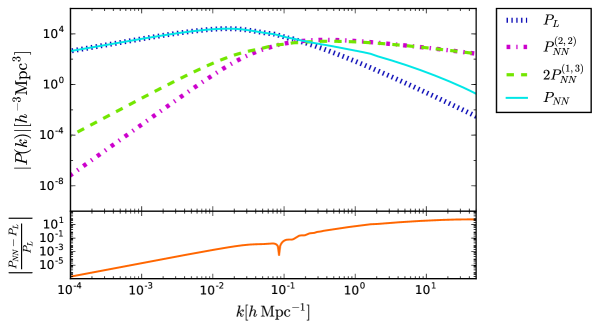
Figure 1: Upper panel: The total Newtonian one-loop power spectrum $P_{NN}$ and the individual second order density power spectrum contributions to the total Newtonian one-loop power spectrum $P^{(2,2)}_{NN}$ and $P^{(1,3)}_{NN}$, at redshift $z=0$. Bottom panel: The relative difference of the Newtonian one-loop power spectrum with respect to the linear power spectrum normalised with the linear power spectrum.

The total relativistic one-loop power spectrum is defined as

$$P_{RR}(k,\eta)=P_{L}(k,\eta)+2P_{RR}^{(1,3)}(k,\eta)+P_{RR}^{(2,2)}(k,\eta).$$ (4.11)

In Figure 2 we present the relativistic results, we show the relativistic contributions to the one-loop power spectrum coming from, $P_{RR}^{(2,2)}$ and $P_{RR}^{(1,3)}$, along with the total relativistic one-loop power spectrum $P_{RR}$, in this Figure we consider the case in where $f_{\rm NL}=g_{\rm NL}=0.$ The relative difference of the relativistic one-loop power spectrum with respect to the linear power spectrum is also shown. We note that relativistic one-loop power spectrum corrections are relevant in the large scales, the relativistic contributions are subdominant in smaller scales.

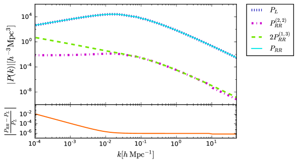
Figure 2: Upper panel: The total relativistic one-loop power spectrum $P_{RR}$ and the individual second order density power spectrum contributions to the total relativistic one-loop power spectrum $P^{(2,2)}_{RR}$ and $P^{(1,3)}_{RR}$ for $f_{\rm NL}=g_{\rm NL}=0$, at redshift $z=0$. Bottom panel: The relative difference of the relativistic one-loop power spectrum with respect to the linear power spectrum normalised with the linear power spectrum.

Finally, the total one-loop power spectrum defined in Eq. (4.2) reads as

$$P_{RN}(k,\eta)=P_{L}(k,\eta)+2P^{(1,3)}(k,\eta)+P^{(2,2)}(k,\eta).$$ (4.12)

In Figure 3 we present a comparison of the total Newtonian one-loop power spectrum $P_{NN}$, the total relativistic one-loop power spectrum $P_{RR}$, along with the total one-loop power spectrum $P_{RN}$, in this Figure we consider the case with no primordial non-Gaussianity $f_{\rm NL}=g_{\rm NL}=0.$ The difference of the total one-loop power spectrum $P_{RN}$ respect to the linear power spectrum $P_{L}$ lies in the large scales is due to the relativistic corrections, whereas the difference in the small scales is given purely by the Newtonian contributions.

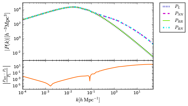
Figure 3: Upper panel: Total Newtonian one-loop power spectrum $P_{NN}$ along with the total relativistic one-loop power spectrum $P_{RR}$ and total one-loop power spectrum $P_{RN}$, with $f_{\rm NL}=g_{\rm NL}=0$, at redshift $z=0$. Bottom panel: Relative difference of the total one-loop power spectrum with respect to the linear power spectrum normalised with the linear power spectrum.

In Figure 4 we present the total one-loop power spectrum $P_{RN}$, using different combinations of values of $f_{\rm NL}$ and $g_{\rm NL}$ reported in by the Planck collaboration in Ref. [48]. The current constraints are given by $f^{\rm local}_{\rm NL}=-0.9\pm 5.1$ and $g^{\rm local}_{\rm NL}=-5.8\pm 6.5\times 10^{4}$. For $f_{\rm NL}$ we use the minimum and maximum values allowed by Planck i.e. $f_{\rm NL}=-6.0$ and $f_{\rm NL}=4.2$. In the case of $g_{\rm NL}$, we use the minimum value allowed by Planck i.e. $g_{\rm NL}=-12.3\times 10^{4}$, however the maximum value of $g_{\rm NL}$ that we can use is $\sim 7$ as higher values, although allowed by the Planck collaboration [48], give negative, non-perturbative contributions to the density power spectrum on large scales. These values for $g_{\rm NL}$ and $f_{\rm NL}$ were chosen to show which values of $f_{\rm NL}$ and $g_{\rm NL}$ have a more significant contribution to the one-loop power spectrum. The relative difference with respect to the linear power spectrum shows that the largest corrections to the power spectrum in the large scales are present when $g_{\rm NL}$ takes its minimum value, being this the dominant correction term as is not affected by the chosen value of $f_{\rm NL}$. On the other hand, larger values of $g_{\rm NL}$ present a similar behaviour for the different combinations with $f_{\rm NL}$, having a small relative difference with respect to the linear power spectrum in comparison to the corrections given by minimum values of $g_{\rm NL}$.

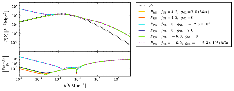
Figure 4: Upper panel: Total one-loop power spectrum $P_{RN}$, at redshift $z=0$, for different limiting values of $f_{\rm NL}$ and $g_{\rm NL}$ reported by Planck[48]. Bottom panel: Relative difference of the relativistic one-loop power spectrum with respect to the linear power spectrum normalised with the linear power spectrum.

In Figure 5 we present the same set of total one-loop power spectrum $P_{RN}$ plots as in Figure 4 but at a redshift $z=1$. In addition to the density power spectrum $P_{RN}$ we also present in the blue shaded area the measurement errors assuming a cosmic variance limited Stage-IV galaxy survey like DESI [1], Euclid [70], or LSST [71]. More specifically, we have assumed a sky area of $15,000\,{\rm deg}^{2}$ at $z=1$ with bin width $\Delta z=0.2$. These numbers correspond to typical specifications of such surveys used in recent forecast and model validation studies at $z=1$ (see e.g. [72]). Note however that the measurement errors would decrease if we chose a wider redshift bin given the large total redshift coverage of Stage IV surveys. Similarly, we have defined the largest measurable scale as $k_{\rm min}\simeq 2\pi/V^{1/3}_{\rm bin}=0.003\,h{\rm Mpc^{-1}}$, where $V_{\rm bin}$ is the volume corresponding to $\Delta z=0.2$; this volume would increase if we were to consider a wider redshift bin, allowing us to reach larger scales. Note that the minimum values of $f_{\rm NL}$ and $g_{\rm NL}$ show the largest impact at the largest measured scales of the upcoming experiments, forecasting a detectability of PNG for values of $g_{\rm NL}$ or $f_{\rm NL}$.

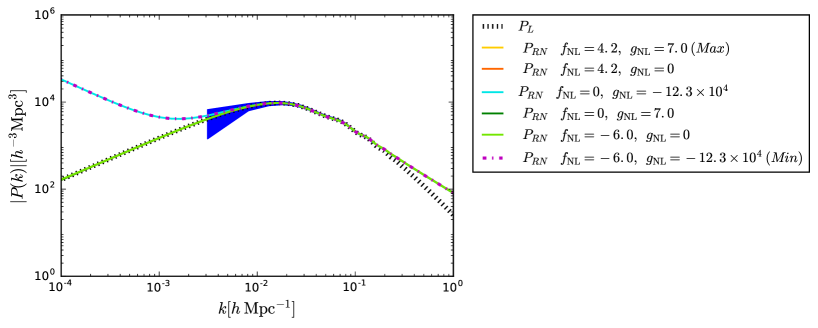
Figure 5: Total one-loop power spectrum $P_{RN}$, at redshift $z=1$, for different limiting values of $f_{\rm NL}$ and $g_{\rm NL}$ reported by Planck [48]. The blue shaded area corresponds to the measurement error of a typical Stage-IV-like survey redshift bin with $\Delta z=0.2$, as detailed in the main text. We also used a $k$-binning $\Delta k=0.006\,h{\rm Mpc^{-1}}$.

5 Tree-level bispectrum

For completeness we calculate the tree-level bispectrum, which is defined as

$$B(k_{1},k_{2},k_{3},\eta)\equiv 2P_{L}(k_{1},\eta)P_{L}(k_{2},\eta)\mathcal{F}^{(2)}(\mathbf{k}_{1},\mathbf{k}_{2})+\rm{(2\enspace cyclic)},$$ (5.1)

the components to calculate the bispectrum at tree-level are already given in Eqs. (3.3) and (3.4). We define the Newtonian tree-level bispectrum $B_{NN}$ as

$$B_{NN}(k_{1},k_{2},k_{3},\eta)\equiv 2P_{L}(k_{1},\eta)P_{L}(k_{2},\eta)\mathcal{F}_{N}^{(2)}(\mathbf{k}_{1},\mathbf{k}_{2})+\rm{(2\enspace cyclic)},$$ (5.2)

and the relativistic tree-level bispectrum as

$$B_{RR}(k_{1},k_{2},k_{3},\eta)\equiv 2P_{L}(k_{1},\eta)P_{L}(k_{2},\eta)\mathcal{F}_{R}^{(2)}(\mathbf{k}_{1},\mathbf{k}_{2})+\rm{(2\enspace cyclic)},$$ (5.3)

the total tree-level bispectrum $B_{RN}$, is defined by Eq. (5.1), where $\mathcal{F}^{(2)}(\mathbf{k}_{1},\mathbf{k}_{2},\eta)$ is given in Eq. (3.2).

In Figure 6 we present a comparison of the Newtonian tree-level bispectrum $B_{NN}$, the relativistic tree-level bispectrum given by $B_{RR}$ and the total tree-level bispectrum $B_{RN}$, all in the squeezed limit, with $\Delta k=0.013\>h\rm{Mpc}^{-1}$ when $f_{\rm NL}=0$ and for the limiting values of $f_{\rm NL}$ given by Ref. [48], the relative difference of the total tree-level bispectrum with respect to the Newtonian bispectrum is shown in the bottom panels. The relativistic corrections at this level are subdominant with respect to the Newtonian tree-level bispectrum.

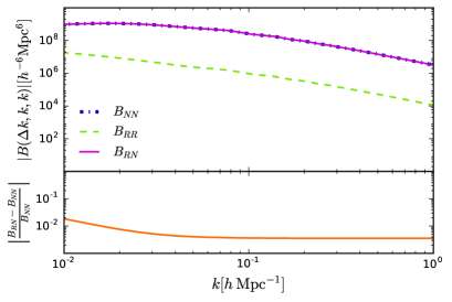
(a)

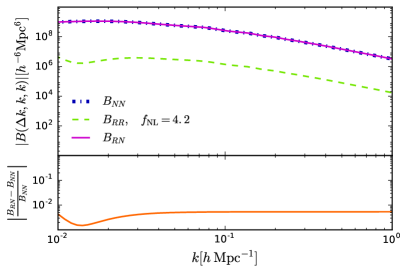
(b)

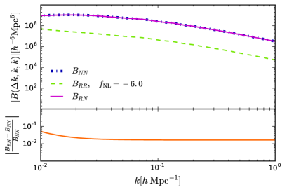
(c)

Figure 6: Upper panels: Comparison of the Newtonian, relativistic and total tree-level bispectrum corrections in the squeezed limit with $\Delta k=0.013\>h\rm{Mpc}^{-1}$ for (a) $f_{\rm NL}=0$, (b) $f_{\rm NL}=4.2$ and (c) $f_{\rm NL}=-6.0$, at redshift $z=0$. Bottom panels: Relative difference of the total tree-level bispectrum with respect to the Newtonian tree-level bispectrum normalised with the Newtonian tree-level.

6 Discussion

We calculated purely general relativistic corrections to the density power spectrum at one-loop. For the synchronous-comoving gauge the primordial non-Gaussianity of the local type can be added naturally and we have also computed the contribution of these parameters. The modifications that relativistic contributions bring to the density power spectrum are below $0.01\%$ except at very large scales where we find a $1\%$ pure relativistic contribution (see Figure 2). On the other hand, the primordial non-Gaussianity values allowed by the latest Cosmic Microwave Background observations in the local configuration yield significant contributions mostly from the $g_{\rm NL}$ parameter (see Figure 5).

The relativistic terms contributing to the higher order amplitude of the density contrast have been derived from a long-wavelength approximation and do not account for effects at all scales. However, it is expected that at small scales the weak field and therefore the Newtonian regime describe best the matter structure. As mentioned above, it is precisely at the large scales where primordial non-Gaussianity contributes to the density power spectrum. Therefore, the formalism employed here to derive relativistic contributions is naturally extended to include the dominant PNG contributions to the density contrast and its polispectra.

The actual corrections from GR to the non-linear bias of galaxies seem to remove the GR effects presented here, however the form of the volume distortions reproduce the form of those expressed in our non-linear prescriptions for the density contrast—at least at second order [11] but decoupling large and short scales—. Yet the local primordial non-Gaussianity terms cannot be removed by local coordinate transformations [12], and terms with such factors are precisely what dominates the signal in the one-loop spectra. It is also important to mention that the GR effects removed by the coordinate transformation are carried at second order and the third order effects described here might survive the coordinate changes. The details of adapting the expressions coming from the volume distortions as galaxies evolve from an initial time, and the precise consequences for a non-linear galaxy power spectrum are left for future work.

Our results show that pure relativistic corrections $P_{RR}$ have a too small contribution at too large scales to be observed in the present or future large scale structure probes. On the other hand, the primordial non-Gaussianity contributions, corresponding to values within the 1-$\sigma$ amplitudes of $g_{\rm NL}$ allowed by Planck [48], yield a significant contribution to $\delta^{(3)}$, and to the one-loop power spectrum observable in the next generation of galaxy surveys. While the deviations from the linear prescription lie within the cosmic variance errors, it may be possible to probe these values through cross-correlations of the future surveys with the measurements of anisotropies in the Cosmic Microwave Background. We shall explore the implications of this effect in order to constrain primordial non-Gaussianity through this and other methods in a future work.

Appendix A Infrared limits

The infrared (IR) contributions of the one-loop integrals (4.6) and (4.9) can be computed as the part of the integral from $r=0$ to a small value $\epsilon$. With this consideration, the one-loop power spectrum can be written as:

$$P^{(2,2)}(k,\eta) = \frac{k^{3}}{2\pi^{2}}\left(\int_{0}^{\epsilon}+\int_{\epsilon}^{\infty}\right)r^{2}drP_{L}(kr,\eta)\int_{-1}^{1}dxP_{L}(k\sqrt{1+r^{2}-2rx},\eta)$$ (A.1)

$$\times\left[(\mathcal{F}^{(2)}_{N})^{2}+2\mathcal{F}^{(2)}_{N}\mathcal{F}^{(2)}_{R}+(\mathcal{F}^{(2)}_{R})^{2}\right]\,,$$

$$P^{(1,3)}(k,\eta) = \frac{k^{3}}{4\pi^{2}}P_{L}(k,\eta)\left(\int_{0}^{\epsilon}+\int_{\epsilon}^{\infty}\right)drP_{L}(kr,\eta)\left[\mathcal{F}^{(3)}_{N}+\mathcal{F}^{(3)}_{R}\right]\,,$$ (A.2)

where the integrals in $r$ have been split between a possible divergent infrared contribution from 0 to $\epsilon$ and a finite contribution from $\epsilon$ to $\infty$ which, in the limit of $\epsilon\to 0$ will correspond to the Cauchy principal value of the integral. Using $P_{L}(k,\eta)\propto k^{n_{s}}$ as $k\to 0$ the infrared contributions can be computed analytically, which we will write explicitly in the following expressions. Note that, in the cases where the integrals diverge we will write the expressions as the limit

$$\int_{0}^{\epsilon}=\lim_{\delta\to 0}\int_{\delta}^{\epsilon}\,,$$ (A.3)

in order to see divergence rate. For the three different terms in $P^{(2,2)}$ we obtain the expressions:

$${}_{\rm{IR}}P^{(2,2)}_{NN} = \frac{k^{3}}{2\pi^{2}}P_{L}(k)P_{L}(k\epsilon)\frac{\epsilon}{3(n_{s}+1)}\,,$$ (A.4)

$${}_{\rm{IR}}P^{(2,2)}_{C} = \frac{\mathcal{H}^{2}k}{2\pi^{2}}P_{L}(k)P_{L}(k\epsilon)\frac{\epsilon}{n_{s}+1}\left(\frac{27}{7}f_{\rm NL}-\frac{95}{42}\right)\,,$$ (A.5)

$${}_{\rm{IR}}P^{(2,2)}_{RR} = \frac{\mathcal{H}^{4}}{2\pi^{2}k}P_{L}(k)P_{L}(k\epsilon)\left(\frac{\epsilon A}{(n_{s}+1)}+\frac{B}{\epsilon(n_{s}-1)}\lim_{\delta\to 0}\left(1-\left(\frac{\delta}{\epsilon}\right)^{n_{s}-1}\right)\right)\,,$$ (A.6)

where

$$A = 9f_{\rm NL}^{2}-\frac{35}{2}f_{\rm NL}+\frac{725}{27}\,,$$ (A.7)

$$B = \frac{(3f_{\rm NL}-5)^{2}}{2}\,.$$ (A.8)

In these expressions the value of $\epsilon$ is small but fixed, meaning that the purely relativistic term diverges approximately as $\delta^{-0.03}$ for $\delta\to 0$. Meanwhile the infrared contributions to $P^{(1,3)}$ read:

$${}_{\rm{IR}}P^{(1,3)}_{NN} = -\frac{k^{3}}{4\pi^{2}}P_{L}(k)P_{L}(k\epsilon)\frac{\epsilon}{3(n_{s}+1)}\,,$$ (A.9)

$${}_{\rm{IR}}P^{(1,3)}_{RR} = \frac{\mathcal{H}^{4}}{4\pi^{2}k}P_{L}(k)P_{L}(k\epsilon)\left(\frac{\epsilon C}{(n_{s}+1)}+\frac{D}{\epsilon(n_{s}-1)}\lim_{\delta\to 0}\left(1-\left(\frac{\delta}{\epsilon}\right)^{n_{s}-1}\right)\right)\,,$$ (A.10)

where

$$C = 54\left(-g_{\rm NL}-\frac{5}{6}f_{\rm NL}-\frac{175}{108}\right)\,,$$ (A.11)

$$D = -\frac{27}{2}\left(-g_{\rm NL}+\frac{10}{3}f_{\rm NL}-\frac{50}{27}\right)\,.$$ (A.12)

We see that the second term in (A.10) diverges at the same rate as (A.6). For the purely Newtonian one loop contribution, the possible infrared problems in the different terms get solved as the combination $2{}_{\rm{IR}}P_{NN}^{(1,3)}(k,\eta)+{}_{\rm{IR}}P_{NN}^{(2,2)}(k,\eta)$ cancels out, as read from the expressions (A.4) and (A.9) (see Ref. [73]). However for the relativistic term this does not happen as the expressions (A.10) and (A.6) do not cancel.

In order to obtain finite results for the relativistic one-loop contribution, we set a lower limit different from zero in the $r$ integrals. The fact that the divergence is very slow allows the results to not be very dependent on this limit, but only as $r_{c}^{-0.03}$. Moreover, as stated in Ref. [8], the observations have a minimum $k$ accessible to them, corresponding to their maximum observed scale. Throughout this work we chose this limit to be in the parameter $q=kr$ as $q_{c}=10^{-5}h{\rm Mpc^{-1}}$ which is close to the limit chosen in Ref. [8] as $q_{c}=H_{0}\approx 3\times 10^{-4}h{\rm Mpc^{-1}}$.

References

- [1] DESI collaboration, The DESI Experiment Part I: Science,Targeting, and Survey Design, 1611.00036.
- [2] EUCLID collaboration, Euclid Definition Study Report, 1110.3193.
- [3] N. Makino, M. Sasaki and Y. Suto, Analytic approach to the perturbative expansion of nonlinear gravitational fluctuations in cosmological density and velocity fields, Phys. Rev. D46 (1992) 585.
- [4] B. Jain and E. Bertschinger, Second order power spectrum and nonlinear evolution at high redshift, Astrophys. J. 431 (1994) 495 [astro-ph/9311070].
- [5] F. Bernardeau, S. Colombi, E. Gaztañaga and R. Scoccimarro, Large scale structure of the universe and cosmological perturbation theory, Phys. Rept. 367 (2002) 1 [astro-ph/0112551].
- [6] C. Bonvin and R. Durrer, What galaxy surveys really measure, Phys. Rev. D84 (2011) 063505 [1105.5280].
- [7] A. Challinor and A. Lewis, The linear power spectrum of observed source number counts, Phys. Rev. D84 (2011) 043516 [1105.5292].
- [8] L. Castiblanco, R. Gannouji, J. Noreña and C. Stahl, Relativistic cosmological large scale structures at one-loop, JCAP 1907 (2019) 030 [1811.05452].
- [9] M. Bruni, R. Crittenden, K. Koyama, R. Maartens, C. Pitrou and D. Wands, Disentangling non-Gaussianity, bias and GR effects in the galaxy distribution, Phys. Rev. D85 (2012) 041301 [1106.3999].
- [10] D. Bertacca, N. Bartolo, M. Bruni, K. Koyama, R. Maartens, S. Matarrese et al., Galaxy bias and gauges at second order in General Relativity, Class. Quant. Grav. 32 (2015) 175019 [1501.03163].
- [11] O. Umeh, K. Koyama, R. Maartens, F. Schmidt and C. Clarkson, General relativistic effects in the galaxy bias at second order, JCAP 1905 (2019) 020 [1901.07460].
- [12] O. Umeh and K. Koyama, The galaxy bias at second order in general relativity with Non-Gaussian initial conditions, JCAP 1912 (2019) 048 [1907.08094].
- [13] J. Calles, L. Castiblanco, J. Noreña and C. Stahl, From matter to galaxies: General relativistic bias for the one-loop bispectrum, 1912.13034.
- [14] J. Adamek, D. Daverio, R. Durrer and M. Kunz, gevolution: a cosmological N-body code based on General Relativity, JCAP 1607 (2016) 053 [1604.06065].
- [15] C. Barrera-Hinojosa and B. Li, GRAMSES: a new route to general relativistic -body simulations in cosmology - I. Methodology and code description, 1905.08890.
- [16] E. Bentivegna and M. Bruni, Effects of nonlinear inhomogeneity on the cosmic expansion with numerical relativity, Phys. Rev. Lett. 116 (2016) 251302 [1511.05124].
- [17] D. Jeong, F. Schmidt and C. M. Hirata, Large-scale clustering of galaxies in general relativity, Phys. Rev. D 85 (2012) 023504.
- [18] C. Bonvin and R. Durrer, What galaxy surveys really measure, Phys. Rev. D 84 (2011) 063505.
- [19] A. Challinor and A. Lewis, Linear power spectrum of observed source number counts, Phys. Rev. D 84 (2011) 043516.
- [20] S. Chen and D. J. Schwarz, Fluctuations of differential number counts of radio continuum sources, Phys. Rev. D91 (2015) 043507 [1407.4682].
- [21] J. Yoo, A. L. Fitzpatrick and M. Zaldarriaga, New perspective on galaxy clustering as a cosmological probe: General relativistic effects, Phys. Rev. D 80 (2009) 083514 [0907.0707].
- [22] D. Bertacca, R. Maartens and C. Clarkson, Observed galaxy number counts on the lightcone up to second order: I. Main result, Journal of Cosmology and Astroparticle Physics 2014 (2014) 037.
- [23] D. Bertacca, R. Maartens and C. Clarkson, Observed galaxy number counts on the lightcone up to second order: II. Derivation, Journal of Cosmology and Astroparticle Physics 2014 (2014) 013.
- [24] E. Di Dio, R. Durrer, G. Marozzi and F. Montanari, Galaxy number counts to second order and their bispectrum, JCAP 1412 (2014) 017 [1407.0376].
- [25] J. Yoo, General relativistic description of the observed galaxy power spectrum: Do we understand what we measure?, Phys. Rev. D 82 (2010) 083508.
- [26] J. Yoo and M. Zaldarriaga, Beyond the Linear-Order Relativistic Effect in Galaxy Clustering: Second-Order Gauge-Invariant Formalism, Phys. Rev. D90 (2014) 023513 [1406.4140].
- [27] J. Yoo and F. Scaccabarozzi, Unified Treatment of the Luminosity Distance in Cosmology, JCAP 1609 (2016) 046 [1606.08453].
- [28] J. T. Nielsen and R. Durrer, Higher order relativistic galaxy number counts: dominating terms, JCAP 1703 (2017) 010 [1606.02113].
- [29] G. Fanizza, J. Yoo and S. G. Biern, Non-linear general relativistic effects in the observed redshift, 1805.05959.
- [30] J. L. Fuentes, J. C. Hidalgo and K. A. Malik, Galaxy number counts at second order: an independent approach, 1908.08400.
- [31] O. Umeh, S. Jolicoeur, R. Maartens and C. Clarkson, A general relativistic signature in the galaxy bispectrum: the local effects of observing on the lightcone, JCAP 1703 (2017) 034 [1610.03351].
- [32] S. Jolicoeur, O. Umeh, R. Maartens and C. Clarkson, Imprints of local lightcone projection effects on the galaxy bispectrum. Part II, JCAP 1709 (2017) 040 [1703.09630].
- [33] C. Clarkson, E. M. de Weerd, S. Jolicoeur, R. Maartens and O. Umeh, The dipole of the galaxy bispectrum, Mon. Not. Roy. Astron. Soc. 486 (2019) L101 [1812.09512].
- [34] E. Mitsou, J. Yoo, R. Durrer, F. Scaccabarozzi and V. Tansella, Angular -point spectra and cosmic variance on the light-cone, 1905.01293.
- [35] R. Maartens, S. Jolicoeur, O. Umeh, C. Clarkson, S. Camera and E. M. De Weerd, Detecting the relativistic galaxy bispectrum, 1911.02398.
- [36] D. Bertacca, A. Raccanelli, N. Bartolo, M. Liguori, S. Matarrese and L. Verde, Relativistic wide-angle galaxy bispectrum on the light-cone, Phys. Rev. D97 (2018) 023531 [1705.09306].
- [37] N. Bartolo, S. Matarrese and A. Riotto, Signatures of primordial non-Gaussianity in the large-scale structure of the Universe, JCAP 0510 (2005) 010 [astro-ph/0501614].
- [38] R. de Putter, O. Doré and D. Green, Is There Scale-Dependent Bias in Single-Field Inflation?, JCAP 1510 (2015) 024 [1504.05935].
- [39] N. Bartolo, D. Bertacca, M. Bruni, K. Koyama, R. Maartens, S. Matarrese et al., A relativistic signature in large-scale structure, Phys. Dark Univ. 13 (2016) 30 [1506.00915].
- [40] V. Desjacques and U. Seljak, Primordial non-Gaussianity from the large scale structure, Class. Quant. Grav. 27 (2010) 124011 [1003.5020].
- [41] N. Bartolo, E. Komatsu, S. Matarrese and A. Riotto, Non-Gaussianity from inflation: Theory and observations, Phys. Rept. 402 (2004) 103 [astro-ph/0406398].
- [42] T. Giannantonio, C. Porciani, J. Carron, A. Amara and A. Pillepich, Constraining primordial non-Gaussianity with future galaxy surveys, Mon. Not. Roy. Astron. Soc. 422 (2012) 2854 [1109.0958].
- [43] A. Taruya, K. Koyama and T. Matsubara, Signature of Primordial Non-Gaussianity on Matter Power Spectrum, Phys. Rev. D78 (2008) 123534 [0808.4085].
- [44] V. Desjacques, U. Seljak and I. Iliev, Scale-dependent bias induced by local non-Gaussianity: A comparison to N-body simulations, Mon. Not. Roy. Astron. Soc. 396 (2009) 85 [0811.2748].
- [45] M. Tellarini, A. J. Ross, G. Tasinato and D. Wands, Galaxy bispectrum, primordial non-Gaussianity and redshift space distortions, JCAP 1606 (2016) 014 [1603.06814].
- [46] E. Di Dio, H. Perrier, R. Durrer, G. Marozzi, A. Moradinezhad Dizgah, J. Noreña et al., Non-Gaussianities due to Relativistic Corrections to the Observed Galaxy Bispectrum, JCAP 1703 (2017) 006 [1611.03720].
- [47] K. Koyama, O. Umeh, R. Maartens and D. Bertacca, The observed galaxy bispectrum from single-field inflation in the squeezed limit, JCAP 1807 (2018) 050 [1805.09189].
- [48] Planck collaboration, Planck 2018 results. IX. Constraints on primordial non-Gaussianity, 1905.05697.
- [49] H. A. Gressel and M. Bruni, fNL-gNL mixing in the matter density field at higher orders, JCAP 1806 (2018) 016 [1712.08687].
- [50] M. Bruni, J. C. Hidalgo and D. Wands, Einstein’s signature in cosmological large-scale structure, Astrophys. J. 794 (2014) L11 [1405.7006].
- [51] M. Bruni, J. C. Hidalgo, N. Meures and D. Wands, Non-Gaussian Initial Conditions in CDM: Newtonian, Relativistic, and Primordial Contributions, Astrophys. J. 785 (2014) 2 [1307.1478].
- [52] N. Meures, General Relativistic Effects on Cosmological Observations, Ph.D. thesis, University of Portsmouth, 2012.
- [53] K. A. Malik and D. Wands, Cosmological perturbations, Phys. Rept. 475 (2009) 1 [0809.4944].
- [54] P. Carrilho and K. A. Malik, Vector and tensor contributions to the curvature perturbation at second order, JCAP 1602 (2016) 021 [1507.06922].
- [55] D. S. Salopek and J. R. Bond, Nonlinear evolution of long wavelength metric fluctuations in inflationary models, Phys. Rev. D42 (1990) 3936.
- [56] D. H. Lyth, K. A. Malik and M. Sasaki, A General proof of the conservation of the curvature perturbation, JCAP 0505 (2005) 004 [astro-ph/0411220].
- [57] D. H. Lyth and A. R. Liddle, The primordial density perturbation: Cosmology, inflation and the origin of structure. Cambridge University Press, Cambridge U.K., (2009).
- [58] E. M. Lifshitz and I. M. Khalatnikov, Investigations in relativistic cosmology, Adv. Phys. 12 (1963) 185.
- [59] K. Tomita, Evolution of Irregularities in a Chaotic Early Universe, Prog. Theor. Phys. 54 (1975) 730.
- [60] C. Rampf and G. Rigopoulos, Zel’dovich Approximation and General Relativity, Mon. Not. Roy. Astron. Soc. 430 (2013) L54 [1210.5446].
- [61] C. Rampf and G. Rigopoulos, Initial conditions for cold dark matter particles and General Relativity, Phys. Rev. D87 (2013) 123525 [1305.0010].
- [62] N. Deruelle and D. Langlois, Long wavelength iteration of Einstein’s equations near a space-time singularity, Phys. Rev. D52 (1995) 2007 [gr-qc/9411040].
- [63] R. M. Wald, General Relativity. Chicago Univ. Pr., Chicago, USA, 1984, 10.7208/chicago/9780226870373.001.0001.
- [64] A. J. Christopherson, J. C. Hidalgo, C. Rampf and K. A. Malik, Second-order cosmological perturbation theory and initial conditions for -body simulations, Phys. Rev. D93 (2016) 043539 [1511.02220].
- [65] J. Carlson, M. White and N. Padmanabhan, A critical look at cosmological perturbation theory techniques, Phys. Rev. D80 (2009) 043531 [0905.0479].
- [66] D. Jeong, Cosmology with high () redshift galaxy surveys, Ph.D. thesis, The University of Texas at Austin, 2010.
- [67] R. Scoccimarro and J. Frieman, Loop corrections in nonlinear cosmological perturbation theory 2. Two point statistics and selfsimilarity, Astrophys. J. 473 (1996) 620 [astro-ph/9602070].
- [68] J. Lesgourgues, The Cosmic Linear Anisotropy Solving System (CLASS) I: Overview, 1104.2932.
- [69] Planck collaboration, Planck 2015 results. XIII. Cosmological parameters, Astron. Astrophys. 594 (2016) A13 [1502.01589].
- [70] Euclid collaboration, Euclid preparation: VII. Forecast validation for Euclid cosmological probes, 1910.09273.
- [71] LSST Dark Energy Science collaboration, Core Cosmology Library: Precision Cosmological Predictions for LSST, Astrophys. J. Suppl. 242 (2019) 2 [1812.05995].
- [72] K. Markovic, B. Bose and A. Pourtsidou, Assessing non-linear models for galaxy clustering I: unbiased growth forecasts from multipole expansion, 1904.11448.
- [73] J. E. McEwen, X. Fang, C. M. Hirata and J. A. Blazek, FAST-PT: a novel algorithm to calculate convolution integrals in cosmological perturbation theory, JCAP 1609 (2016) 015 [1603.04826].