On the costs and profit of software defect prediction

Abstract

Defect prediction can be a powerful tool to guide the use of quality assurance resources. However, while lots of research covered methods for defect prediction as well as methodological aspects of defect prediction research, the actual cost saving potential of defect prediction is still unclear. Within this article, we close this research gap and formulate a cost model for software defect prediction. We derive mathematically provable boundary conditions that must be fulfilled by defect prediction models such that there is a positive profit when the defect prediction model is used. Our cost model includes aspects like the costs for quality assurance, the costs of post-release defects, the possibility that quality assurance fails to reveal predicted defects, and the relationship between software artifacts and defects. We initialize the cost model using different assumptions, perform experiments to show trends of the behavior of costs on real projects. Our results show that the unrealistic assumption that defects only affect a single software artifact, which is a standard practice in the defect prediction literature, leads to inaccurate cost estimations. Moreover, the results indicate that thresholds for machine learning metrics are also not suited to define success criteria for software defect prediction.

1 Introduction

Research regarding software defect prediction for the accurate prediction of post-release defects in software is an ongoing and still unresolved research topic, that was already discussed in hundreds of publications [1, 2, 3]. Current research focuses on problems like cross-project defect prediction (e.g., [4]), heterogeneous defect prediction (e.g., [5, 6]), unsupervised defect prediction (e.g., [7, 8]), and just-in-time defect prediction (e.g., [9]). Additionally, researchers have turned their attention to how defect prediction research should be conducted, e.g., reducing the bias through sampling approaches [10], the impact of hyper parameter tuning [11], suitable baseline comparisons [12] or general guidelines that should be considered [13]. While all of the above contribute to the advancement of the defect prediction state of the art, there are also multiple publications that question the progress of the state of the art through replications in recent years, as they demonstrate that older (e.g., [4]) or trivial (e.g., [14, 15]) approaches are comparable too or even better than more complex recent approaches from the state of the art.

The problems with replications of prior results lead to the question, if defect prediction can currently really help developers and organizations to reduce costs. While this aspect is crucial, there are only few publications that cover cost models for defect prediction (see Section 2). Moreover, the existing cost models have several limitations, e.g., a 1-to-1 relationship between software artifacts and defects, or the assumption that quality assurance is perfect, i.e., all predicted defects are found. Additionally, researchers often use of “standard” machine learning metrics like precision, recall, F-Measure, MCC, AUC and others instead of a cost model [3, 16]. While these metrics are suitable to estimate the general performance of defect prediction models, they are not suitable to answer the question if defect prediction can actually save costs, i.e., have a positive profit.

With this article, we want to close this research gap through the specification of a general cost model for defect prediction. Our cost model takes the costs for quality assurance, the costs of defects, the relationship between defects and software artifacts, the possibility that quality assurance may fail to reveal defects as well as one-time and continuous costs for the execution of the defect prediction into account.

The contributions of this article are the following:

• A general cost model for software defect prediction.

• Mathematically proven boundary conditions on cost saving defect predictions.

• Initializations of the cost model with realistic assumptions that can be used by researchers and practitioners for the evaluation of defect prediction models, including guidelines on how to use the cost model.

• Through the work on the cost model, we discovered a principle problem in current defect prediction papers, i.e., that we do not account for the fact that there is an $n$-to-$m$ relationship between software artifacts and defects. Through simulations of defect prediction models on real-world data, we have shown that the results, especially in terms of costs, may change if this relationship is considered.

The remainder of this article is structured as follows. In Section 2 we discuss existing cost models and cost-sensitive metrics for software defect prediction. Then, we formally specify the problem of software defect prediction in Section 3 and derive the general cost model for defect prediction from this specification in Section 4. In Section 5 we proof properties that must be fulfilled by defect prediction models in order to have a positive profit. Then, we show how the general cost model can be initialized under different assumptions in Section 6. Through simulation experiments, we evaluate trends of the boundary conditions for cost saving defect predictions, as well as the impact of different assumptions on the initialization of the cost model in Section 7. We proceed with a discussion of our cost model, including guidelines on how to use our model and threats to the validity of our work in Section 8 and conclude in Section 9.

2 Related Work

Most of the defect prediction literature does not use cost-sensitive evaluations, but standard machine learning measures based on the confusion matrix, e.g., precision, recall, F-Measure, and MCC. Within this section, we discuss approaches for the evaluation of defect prediction models that directly take costs into account. We differentiate between cost metrics and cost models. A cost metric takes specific parts of the costs into account, but does not try to actually estimate the complete costs related to the defect prediction model. A cost model combines multiple or all relevant aspects associated with the costs of a defect prediction model. As a consequence, cost metrics are only indicators of cost effectiveness, whereas cost models can be used to calculate the costs as well as the profit of defect prediction models. After the discussion of costs models for defect prediction, we present a broader overview about related work on cost modeling, both in software engineering as well as other domains.

2.1 Cost Metrics

There are also multiple performance metrics in the literature, which take costs into account. Ohlson and Alberg [17], as well as Rahman et al. [18] defined variants of Receiver Operating Characteristic (ROC) curves that take costs into account. These ROC curves are defined over the number of defects found versus the number of artifacts that have to be considered. Using the area under this ROC curve, a threshold independent and cost sensitive performance measure is defined. The variant by Ohlson and Alborg is also known as lift chart [19]. Rahman et al. [18] also considered using the percentage of lines of code instead of the number of artifacts. However, the results are similar. Hemmati et al. [20] use a similar variant of ROC that considers the percentage of defects detected versus the percentage of lines of code. Arisholm and Briand [21] propose an approach similar to a ROC curve. They plot the percentage of defects found, as well as the percentage of code considerd both on the y-axis versus different cutoff values for a prediction model on the x-axis. The area between these lines indicates the cost saving potential.

Canfora et al. [22] use costs defined by the lines of code that are predicted as defective as a criterion for a multi-objective optimization algorithm for cross-project defect prediction. Another measure that is considered is the number of modules that must be visited before 80% of the defects are found (e.g., [23]). Similarly, some authors considered the number of defects found if the top twenty percent of the predictions are considered (e.g., [24]), i.e., the predictions with the highest scores.

2.2 Cost Models

A cost model with similar traits to our work was proposed by Khoshgoftaar and Allen [25]. In their work, the authors observe that the costs for false positives and false negatives are different. They model the expected costs of misclassifications through two constants that represent the costs of unnecessary quality assurance in case of false positives and the costs of missed defects in case of false negatives. Later, this approach was extended to consider these costs as a ratio [26]. Drummond and Holte [27] propose the use of cost curves for classifier comparisons. The cost curves consider the same cost model as Khoshgoftaar and Allen [25], i.e. the expected costs of misclassifications. However, instead of assuming a single constant, they propose to use a ROC curve of the expected costs versus different cost ratios.

Another cost model for defect prediction was proposed by Zhang and Cheung [28]. The model is also similar to the work by Khoshgoftaar and Allen [25]. However, they also took the costs for true positives into account, i.e., the costs of necessary quality assurance that can prevent post release defects. Based on this model, the authors derive a criterion for cost-effectiveness of defect prediction that must be fulfilled such that defect prediction outperforms randomly selecting artifacts for quality assurance as well as applying quality assurance to all artifacts.

While our cost model has the same general structure as the models by Khoshgoftaar et al. [25, 26] and Zhang and Cheung [28], both may only be considered as a special case of our approach as they have several limitations which our model overcomes. They assume 1-to-1 relationships between software artifacts and defects, i.e., binary defect labels for the artifacts. This is unrealistic as software artifacts may contain multiple defects and defects may affect multiple software artifacts. Moreover, both models do not take into account that quality assurance is not perfect and may not be able to detect predicted defects. Additionally, the models assume constant costs for both quality assurance as well as defects. Our general model allows individual costs for each artifact and each defect and we cover the constant costs as a special case we consider. Finally, both cost models ignore one-time and continuous costs that occur if a defect prediction model is used within a development process. The cost curves by Drummond and Holte [27] could also be used with our cost model, to visualize the cost savings for different cost ratios.

2.3 Cost Model for Other Applications

While this article is focused on cost models for defect prediction, we also want to give a brief overview on cost models for other applications. In software engineering, similar cost models to our work were proposed for the reliability assessment of software with the goal to determine the time costs of releases [29]. Such models estimate the costs based on the costs for quality assurance and for fixing defects prior to a release in comparison to the costs due to fixing defects after the release and the costs for delaying a release. The reliability models use stochastic processes to model the expected number of defects in the software, e.g., a non-homogeneous Poisson process [30]. Such a stochastic process is not required for our cost model because the defects are known from empirical data. Similar to our work, the cost models for software reliability use constants for the costs of quality assurance and due to defects. The only cost factor that is not assumed as constant are the penalty costs for delaying a release, which are modelled as a function that monotonically increases with the delay.

Stolfo et al. [31] created a cost model for the evaluation of machine learning based fraud detection. While the domain is different, the goal is similar to our work for defect prediction, i.e., to provide means beyond standard machine learning metrics to assess the impact of a prediction approach on costs. The assumptions behind the structure of the cost model are similar to defect prediction cost models. The authors compute the cost savings based on the effort spent due to predictions, costs saved due to true positive predictions of fraud, and false negative misses of fraud. The costs for effort spent is similar to the quality assurance costs in defect prediction cost models and assumed by Stolfo et al. [31] to be constant. The costs for detecting or missing fraud is similar to the costs of defects. A big advantage of the fraud detection cost model over our initializations of the cost model is that the authors know the loss due to fraud, because this is the amount of money in a fraudulent transaction. In comparison, we have to rely on a constant that represents the mean costs per defect.

In general, the literature on cost models follows a pattern for the creation of cost models similar to our work: the authors determine factors related to the costs from the literature and/or experience and create a cost model as the sum of these cost factors. For example, Patry et al. [32] use this approach to assess the cost of lithium-ion battery cells, Etkin [33] assess different factors of costs associated with oil spillages, and Pugliatti et al. [34] for the cost of epilepsy in Europe. We note that the complexity of the cost models is also impacted by the amount of research invested into understanding different cost factors in detail. For example, decades of research on economics have led to complex cost models that can model whole economies by describing different actors through well-understood stochastic processes. An example for such a model is the work by Nakumura and Steinsson [35]: the authors created a cost model that takes household consumptions of different goods over time as well as the labor and production behavior of companies into account to analyze the impact of economic shocks on money non-neutrality.

3 Specification of defect prediction

Defect prediction models are used to assess the risk of software artifacts and guide quality assurance efforts in order to prevent post-release defects. Formally, let $S$ be a software product that consists of artifacts $s\in S$. These artifacts may be modules, files, classes or methods. The software product contains defects $d\in D$, whereas each defect belongs to one or more artifacts. We denote the artifacts that $d$ belongs to as a set and define $d=\{s^{d}_{1},,\ldots,s^{d}_{n}\}$ to denote that the artifacts $s^{d}_{1},\ldots s^{d}_{n}\in S$ are defective because of defect $d$. Vice versa, we denote the defects that affect an artifact $s$ as $d(s)=\{d\in D:s\in d\}$. Since one defect can belong to multiple artifacts, and artifacts can be affected by multiple defects, we have an $n$ to $|d(s)|=m$ relationship between artifacts and defects. Given the defects $D$, we can divide the artifacts $S$ into two disjunctive sets $S_{DEF}$ and $S_{CLEAN}$ such that $S_{DEF}$ contains all artifacts that contain defects and $S_{CLEAN}$ contains all artifacts without any defects, i.e.,

$$\begin{split}S_{DEF}&=\bigcup_{d\in D}d\\ S_{CLEAN}&=S\setminus S_{DEF}.\end{split}$$ (1)

The goal of defect prediction models is to estimate $S_{DEF}$ and $S_{CLEAN}$. Thus, a defect prediction model is a function

$$h:S\rightarrow\{Defective,Clean\}.$$ (2)

In the following, we use the labels $1=Defective$ and $0=Clean$, i.e., the prediction model classifies artifacts into clean and defective artifacts. With the exception of a publication by Hemmati et al. [20], the current state of the art assumes each artifact that is correctly labeled as defective, predicts all defects in that affect an artifact correctly. However, this is not necessarily the case, because a defect $d\in D$ may affect multiple artifacts. A defect $d$ is successfully predicted by a defect prediction model if all artifacts $s\in d$ are labeled as defective, i.e., $h(s)=1$ for all $s\in d$. We define the set of defects that are successfully predicted by a defect prediction model $h$ as

$$D_{PRED}=\{d\in D:\forall s\in d~{}|~{}h(s)=1\}$$ (3)

and the set of defects that are missed as

$$D_{MISS}=\{d\in D:\exists s\in d~{}|~{}h(s)=0\}=D\setminus D_{PRED}$$ (4)

To get a better understanding of our definitions, consider an example with three software artifacts $S=\{s_{1},\ldots,s_{3}\}$ and two defects $D=\{d_{1}=(s_{1}),d_{2}=(s_{1},s_{2})\}$. Thus, $s_{1}$ is affected by both defects, $s_{2}$ is only affected by defect $d_{2}$ and $s_{3}$ is clean. Let us consider a defect prediction model that predicts $s_{1}$ as defective and the other artifacts as clean, i.e., $h(s_{1})=1$, $h(s_{2})=0$, and $h(s_{3})=0$. This means that $D_{PRED}=\{d_{1}\}$ because all artifacts that $d_{1}$ affects are predicted as defective by $h$ and $D_{MISS}=\{d_{2}\}$ because the artifact $s_{2}$ that is affected by $d_{2}$ is predicted as clean.

Depending on the prediction of the model and the actual post-release defects that are observed in the software, there are four possible outcomes of a prediction.

1. The defect prediction model predicts a post-release defect in an artifact correctly. This is called a true postive. We denote the number of true positives as $tp$.

2. The defect prediction model falsely predicts a post-release defect in an artifact. This is called a false positive. We denote the number of false positives as $fp$.

3. The defect prediction model correctly predicts that an artifact does not contain a post-release defect. This is called true negative. We denote the number of true negatives as $tn$.

4. The defect prediction model falsely predicts that an artifact does not contain a post-release defect. This is called a false negative. We denote the number of false negatives as $fn$.

4 General Cost Model

The use of defect prediction models affects several costs in a development process. In general, we must account for the following factors.

• $cost_{INIT}$, i.e., one-time costs for the introduction of defect prediction into a development process.

• $cost_{EXEC}$, i.e., continuous costs related to the usage of the defect prediction model in the development process, e.g, for the preparation of data, analysis of prediction results, or the re-training of models.

• $cost_{QA}$, i.e., costs due to additional quality assurance measures that are applied as a result of the predictions made by the model.

• $cost_{DEF}$, i.e., the costs due to post-release defects. These costs include not only the directly incurring costs, e.g., due to a loss in revenue or contract penalties, but also the maintenance costs for deploying patches in the wild, the costs of regression testing, or costs due to an increased effort for the correction due to restrictions on the allowed changes to the source code after the initial release.

The costs for actually fixing the defects in the artifacts are not a relevant factor for the costs of defect prediction. These costs either occur as a result of quality assurance before the release, or due to a post-release defect after the release. Thus, the costs for fixing a defect will always be present and cannot be changed due to the defect prediction, only losses due to post-release defects can be prevented.

If all the costs are known, we can calculate the costs associated with acting according to a defect prediction model as

$$cost=cost_{INIT}+cost_{EXEC}+cost_{QA}+cost_{DEF}.$$ (5)

4.1 One-time costs and continuous costs

The one-time costs and continuous costs account for the investment required to establish and execute the defect prediction model within a development process. Both the one-time costs and the continuous costs depend on the current development process in an organization, the desired defect prediction model, and how the defect prediction is integrated into the development process. Relevant factors of the current development process are, e.g., the availability of links from work done in a version control system for the source to the issue tracking system in use, as well as established procedures for the static analysis of the software product. The factors that influence the resulting costs of a defect prediction model are similar to those for any change in the development process, e.g., tool costs, training costs, or migration costs. Moreover, there is a trade-off between one-time costs and continuous costs: high one-time costs can reduce the continuous costs. E.g., if a lot of money is spent to create a defect prediction tool that runs fully automated, including aspects like retraining and performance reports, the continuous costs are relatively low in comparison to manual retraining and performance reporting. Regardless, the estimation of the continuous costs should also account for risks, e.g., additional training costs due to developer turnover. Underestimating the risks may result in a too conservative estimate of the continuous costs and, therefore, may require the re-estimation of the continuous costs and a subsequent re-evaluation of the cost effectiveness of the defect prediction model.

This already shows that the one-time and continuous costs are highly dependent on the tool market: if off-the-shelf tools for defect prediction are available, the costs are constant and depend on the licensing model, training costs of the tool provider, as well es potential prior experience with tools by developers.

Moreover, the one-time costs and continuous costs are considered independently from the quality assurance costs and costs of defects. We assume that the one-time and continuous costs are constants that represent the mean of the expected costs for establishing and executing the defect prediction model in an organization, i.e.,

$$cost_{INIT}=C_{INIT}$$ (6)

and

$$cost_{EXEC}=C_{EXEC}.$$ (7)

4.2 Quality assurance costs

These are the costs that result from the prediction of the defect prediction model, i.e., that result from acting upon defective predictions by the model. The costs for the quality assurance measures depend on the techniques for quality assurance (e.g., code reviews, software tests). Moreover, the quality assurance costs may depend on the artifacts themselves and may vary, e.g., due to the artifact size or complexity. The estimate of these costs should take the experience of developers into account and, therefore, may need to be adopted in case of developer turnover. We denote these costs as $qa(s)$. These costs occur for all artifacts that are predicted as defective, i.e.,

$$\begin{split}cost_{QA}&=\sum_{s\in S:h(s)=1}qa(s).\end{split}$$ (8)

We model these costs in relation to the artifacts $S$ and not the defects $D$, because defect prediction models also label artifacts, instead of identifying concrete defects which may be related to a set of artifacts.

4.3 Defect costs

The last component are the costs due to post-release defects $d$, i.e., defects that are not found by the quality assurance and make it into the wild. We denote the costs of each defect as $loss(d)$. The costs due to post-release defects consist of two parts. The first part are the costs due to defects, which are not found because they are not predicted by the model, i.e., $d\in D_{MISS}$. The second part of the costs are due to the imperfection of quality assurance. Even if we predict an artifact as defective and apply quality assurance measures, there is no guarantee that a defect is actually found. We model this chance that quality assurance fails as $qf(d)$ where $qf(d)\in[0,1)$ is the expected value that the defect is not found by the quality assurance. We assume that $qf(d)<1$, i.e., that the quality assurance has a chance to uncover all defects. The expected costs due to defects that are missed by the quality assurance are $qf(d)\cdot loss(d)$ for all artifacts $d\in D_{PRED}$. The expected costs due to post release defects are

$$\begin{split}cost_{DEF}&=\sum_{d\in D_{MISS}}loss(d)\\ &+\sum_{d\in D_{PRED}}qf(d)\cdot loss(d).\end{split}$$ (9)

4.4 Complete general cost model

If we use our definitions from equations (6)-(9) within equation (5), we get

$$\begin{split}cost&=C_{INIT}+C_{EXEC}+\sum_{s\in S:h(s)=1}qa(s)\\ &+\sum_{d\in D_{MISS}}loss(d)+\sum_{d\in D_{PRED}}qf(d)\cdot loss(d).\end{split}$$ (10)

5 Conditions for Cost-Saving Defect Prediction

A still unanswered question in defect prediction research is what it means for a defect prediction model to be good and when defect prediction is actually successful. To our mind a defect prediction is successful, if it saves costs, i.e., has a positive profit. Whether a concrete defect prediction model is cost saving, depends not only on the quality of the predictions, but also on the actual costs of defects and the costs for quality assurance. These costs depend on the project context. Therefore, general statements whether defect prediction models are cost saving or not are impossible. However, if we assume that the costs for defects are a known constant $C$, we can proof boundary conditions on $C$ that must be fulfilled in order for the defect prediction model to have a positive profit. That constant costs $C$ for defects are not unreasonable for practical purposes is discussed in Section 6.3. Within this section, we derive boundary conditions on the costs of defects $C$.

With Theorem 1 we specify boundary conditions that must be fulfilled to have a positive profit in comparison to randomly applying quality assurance to artifacts with probability $p_{qa}$. Theorem 1 specifies the boundary conditions using the fraction of the sum of the costs saved due to predicted defects ($\sum_{d\in D_{PRED}}(qf(d)-1)$) and the costs saved if defects are randomly predicted correctly ($\sum_{d\in D}p_{qa}^{|d|}\cdot(1-qf(d))$) as denominator and the costs for quality assurance for randomly predicted artifacts ($\sum_{s\in S}p_{qa}\cdot qa(s)$) minus the costs of quality assurance due to a defect prediction model ($\sum_{s\in S:h(s)=1}qa(s)-C_{INIT}-C_{EXEC}$) as nominator. Depending on whether this ratio is positive or negative, Theorem 1 defines an upper, respectively lower boundary on the costs of defects.

Theorem 1.

Let $S$ be the artifacts of a software product with post-release defects $D$, $h:S\to\{0,1\}$ a defect prediction model, $qa(s)$ the costs for the quality assurance of artifact $s\in S$, $qf(d)$ the expected value that quality assurances misses a defect $d$, $loss(d)=C$ the costs of a defect. Furthermore, let $p_{qa}$ be the probability that quality assurance is applied to an artifact randomly.

Let

$$\begin{split}x=\sum_{d\in D_{PRED}}(qf(d)-1)+\sum_{d\in D}p_{qa}^{|d|}\cdot(1-qf(d))\end{split}$$ (11)

$$y=\sum_{s\in S}p_{qa}\cdot qa(s)-\sum_{s\in S:h(s)=1}qa(s)-C_{INIT}-C_{EXEC}$$ (12)

The defect prediction model $h$ has an expected positive profit in comparison to the random selection of artifacts with probability $p_{qa}$, if

$$C<\frac{y}{x}~{}\text{if}~{}x>0$$ (13)

respectively

$$C>\frac{y}{x}~{}\text{if}~{}x<0$$ (14)

Proof.

To proof the boundaries on C, we analyze the expected profit of a defect prediction model in comparison to randomly selecting artifacts, which is

$$profit=cost_{random}-cost$$ (15)

where is $cost$ as defined in Equation (10) and $cost_{random}$ are the costs of defect prediction if quality assurance is applied randomly with probability $p_{qa}$. We get the $cost_{random}$ by applying the preconditions of this theorem to Equation (10) and get

$$\begin{split}cost_{random}&=\sum_{s\in S}p_{qa}\cdot qa(s)+\sum_{d\in D}(1-p_{qa}^{|d|})\cdot loss(d)\\ &+\sum_{d\in D}p_{qa}^{|d|}\cdot qf(d)\cdot loss(d).\end{split}$$ (16)

Thus, we have

$$\begin{split}profit&=\sum_{s\in S}p_{qa}\cdot qa(s)+\sum_{d\in D}(1-p_{qa}^{|d|})\cdot loss(d)\\ &+\sum_{d\in D}p_{qa}^{|d|}\cdot qf(d)\cdot loss(d)\\ &-C_{INIT}-C_{EXEC}-\sum_{s\in S:h(s)=1}qa(s)\\ &-\sum_{d\in D_{MISS}}loss(d)-\sum_{d\in D_{PRED}}qf(d)\cdot loss(d).\end{split}$$ (17)

Therefore, the profit is positive, if

$$\begin{split}0&<\sum_{s\in S}p_{qa}\cdot qa(s)+\sum_{d\in D}(1-p_{qa}^{|d|})\cdot loss(d)\\ &+\sum_{d\in D}p_{qa}^{|d|}\cdot qf(d)\cdot loss(d)\\ &-C_{INIT}-C_{EXEC}-\sum_{s\in S:h(s)=1}qa(s)\\ &-\sum_{d\in D_{MISS}}loss(d)-\sum_{d\in D_{PRED}}qf(d)\cdot loss(d).\end{split}$$ (18)

We now move all terms that contain $loss(d)$ to the left-hand side of the equation and get

$$\begin{split}\sum_{d\in D_{MISS}}loss(d)&+\sum_{d\in D_{PRED}}qf(d)\cdot loss(d)\\ -\sum_{d\in D}(1-p_{qa}^{|d|})\cdot loss(d)&-\sum_{d\in D}p_{qa}^{|d|}\cdot qf(d)\cdot loss(d)\\ &<\\ \sum_{s\in S}p_{qa}\cdot qa(s)-C_{INIT}&-C_{EXEC}-\sum_{s\in S:h(s)=1}qa(s)\end{split}$$ (19)

The right-hand side of the equation is now equal to $y$ as defined in Equation (12). For the left-hand side, we use that one of the conditions of our theorem is $loss(d)=C$ and get

$$\begin{split}\sum_{d\in D_{MISS}}C&+\sum_{d\in D_{PRED}}qf(d)\cdot C\\ -\sum_{d\in D}(1-p_{qa}^{|d|})\cdot C&-\sum_{d\in D}p_{qa}^{|d|}\cdot qf(d)\cdot C\\ &<y\end{split}$$ (20)

Because $C$ is independent of the terms of the sums, we can factorize $C$ and get

$$\begin{split}C\cdot\Biggl{(}&\sum_{d\in D_{MISS}}1+\sum_{d\in D_{PRED}}qf(d)\\ &-\sum_{d\in D}(1-p_{qa}^{|d|})-\sum_{d\in D}p_{qa}^{|d|}\cdot qf(d)\Biggr{)}<y.\end{split}$$ (21)

Because $-\sum_{d\in D}(1-p_{qa}^{|d|})=-\sum_{d\in D}1+\sum_{d\in D}p_{qa}^{|d|})$ and $-\sum_{d\in D}1=-\sum_{d\in D_{miss}}1-\sum_{d\in D_{PRED}}1$ it follows that

$$\begin{split}C\cdot\Biggl{(}&\sum_{d\in D_{PRED}}qf(d)-\sum_{d\in D_{PRED}}1\\ &+\sum_{d\in D}p_{qa}^{|d|}-\sum_{d\in D}p_{qa}^{|d|}\cdot qf(d)\Biggr{)}<y\end{split}$$ (22)

We can reformulate this as

$$\begin{split}C\cdot\Biggl{(}\sum_{d\in D_{PRED}}(qf(d)-1)+\sum_{d\in D}p_{qa}^{|d|}\cdot(1-qf(d))\Biggr{)}<y.\end{split}$$ (23)

The left-hand side of the equation is $C\cdot x$ with $x$ as defined in Equation (11). If we divide by $x$, we get our boundary conditions for $C$. ∎

We use Theorem 1 to derive two corollaries. Corollary 1 specifies a lower boundary through not applying additional quality assurance at all, which is the same as a random defect prediction model with probablity $p_{qa}=0$. The resulting boundary condition basically means that the costs saved due to predicted defects must be greater than the costs for the additional quality assurance. Corollary 2 specifies an upper boundary through applying additional quality assurance to all artifacts, which is the same as a random defect prediction model with probability $p_{qa}=1$. The resulting boundary condition basically means that the costs due to missed defects must be lower than the costs for the quality assurance for the artifacts that were not predicted as defective would have been.

Corollary 1.

Let $S$ be the artifacts of a software product with post-release defects $D$, $h:S\to\{0,1\}$ a defect prediction model, $qa(s)$ the costs for the quality assurance of artifact $s\in S$, $qf(d)$ the expected value that quality assurances misses a defect, $loss(d)=C$ the costs of a defect.

The defect prediction model $h$ has a positive profit in comparison to no quality assurance for any artifact $s\in S$ if

$$C>\frac{\sum_{s\in S:h(s)=1}qa(s)+C_{INIT}+C_{EXEC}}{\sum_{d\in D_{PRED}}(1-qf(d))}.$$ (24)

Proof.

No quality assurance is the same as a random approach for defect prediction with $p_{qa}=0$. We use this to calculate $x$ and $y$ from Theorem 1.

For $y$ we get that

$$y=\sum_{s\in S}0\cdot qa(s)-\sum_{s\in S:h(s)=1}qa(s)-C_{INIT}-C_{EXEC}$$ (25)

Because the first term is zero, we get

$$y=-\sum_{s\in S:h(s)=1}qa(s)-C_{INIT}-C_{EXEC}.$$ (26)

For $x$ we get that

$$\begin{split}x=\sum_{d\in D_{PRED}}(qf(d)-1)+\sum_{d\in D}0^{|d|}\cdot(1-qf(d))\end{split}$$ (27)

When we remove the terms that are now zero, we get

$$x=\sum_{d\in D_{PRED}}(qf(d)-1)$$ (28)

Since $qf(d)\in[0,1)$ it follows that $qf(d)-1<0$ and consequently that $x<0$. Thus, Equation (14) applies and we get

$$C>\frac{-\sum_{s\in S:h(s)=1}qa(s)-C_{INIT}-C_{EXEC}}{\sum_{d\in D_{PRED}}(qf(d)-1)}.$$ (29)

We can factorize -1 from the nominator of the right-hand side and then multiply the -1 with the denominator instead and get

$$C>\frac{\sum_{s\in S:h(s)=1}qa(s)+C_{INIT}+C_{EXEC}}{\sum_{d\in D_{PRED}}(1-qf(d))}.$$ (30)

∎

Corollary 2.

Let $S$ be the artifacts of a software product with post-release defects $D$, $h:S\to\{0,1\}$ a defect prediction model, $qa(s)$ the costs for the quality assurance of artifact $s\in S$, $qf(d)$ the expected value that quality assurances misses a defect, $loss(d)=C$ the costs of a defect.

The defect prediction model $h$ has a positive profit in comparison to quality assurance for all artifacts $s\in S$ if

$$C<\frac{\sum_{s\in S:h(s)=0}qa(s)-C_{INIT}-C_{EXEC}}{\sum_{d\in D_{MISS}}(1-qf(d))}.$$ (31)

Proof.

Quality assurance for all artifacts $s\in S$ is the same as a random approach for defect prediction with $p_{qa}=1$. We use this to calculate $x$ and $y$ from Theorem 1.

For $y$ we get that

$$y=\sum_{s\in S}1\cdot qa(s)-\sum_{s\in S:h(s)=1}qa(s)-C_{INIT}-C_{EXEC}$$ (32)

Because $\sum_{s\in S}qa(s)=\sum_{s\in S:h(s)=0}qa(s)+\sum_{s\in S:h(s)=1}qa(s)$, we get

$$y=\sum_{s\in S:h(s)=0}qa(s)-C_{INIT}-C_{EXEC}.$$ (33)

For $x$ we get that

$$\begin{split}x=\sum_{d\in D_{PRED}}(qf(d)-1)+\sum_{d\in D}1^{|d|}\cdot(1-qf(d)).\end{split}$$ (34)

Because $\sum_{d\in D}(1-qf(d))=\sum_{d\in D_{MISS}}(1-qf(d))+\sum_{d\in D_{PRED}}(1-qf(d))$ we get

$$\begin{split}x=\sum_{d\in D_{MISS}}1-\sum_{d\in D_{MISS}}qf(d).\end{split}$$ (35)

We can rewrite this as

$$\begin{split}x=\sum_{d\in D_{MISS}}(1-qf(d)).\end{split}$$ (36)

Since $qf(d)\in[0,1)$ it follows that $1-qf(d)>0$ and consequently $x>0$. Thus, Equation (13) applies and we get

$$C<\frac{\sum_{s\in S:h(s)=0}qa(s)-C_{INIT}-C_{EXEC}}{\sum_{d\in D_{MISS}}(1-qf(d))}.$$ (37)

∎

6 Initializations of the general cost model

To actually initialize our cost model and use it for the computation of costs and concrete values for the boundary conditions on defect costs, we need estimations for $C_{INIT}$, $C_{EXEC}$, $qa(s)$, $qf(s)$, and $loss(d)$. We start this section with a discussion on how each of these costs components may be estimated. Then, we proceed to initialize six concrete cost models from the general costs model including the resulting boundary conditions on the costs of defects.

6.1 One-time and execution costs

In Section 4.1, we already argued that the costs $C_{INIT}$ and $C_{EXEC}$ are rather an issue of the development of a tool market, than of the actual performance of the defect prediction model. Moreover, tooling costs are usually small in comparison to other human resources. Because these costs are likely a minor costs component and not a deciding factor for the introduction of a defect prediction model, we assume these costs to be zero and omit them from the initializations of the general cost model. In case the costs are known for a specific use case, the constants can simply be added to the model again, without major changes. The impact of this decision is further discussed in Section 8.5.

6.2 Cost of quality assurance

For the size-aware cost model, we assume that the costs of quality assurance are a linear function of the size of a software artifact, i.e.,

$$qa_{size}(s)=C_{QA}\cdot size(s)$$ (38)

where $C_{QA}$ is a constant that describes the quality assurance costs per size unit. The idea to measure quality assurance effort in relation to the size of software artifacts is, e.g., also used by Rahman et al. [18] and Canfora et al. [22, 36], who both use the lines of code of the software artifacts as indicator for quality assurance efforts.

In case a simpler approach is wanted or the size of artifacts is not considered a relevant factor, we propose to use constant costs for quality assurance independent of the size, i.e.,

$$qa_{const}(s)=C_{QA}.$$ (39)

The assumption of constant costs is also used, e.g., in the cost models by Khoshgoftaar et al. [25, 26] and Zhang and Cheung [28]. In both cases, the values for the constants in a concrete use of the cost model must be estimated by a member of the organization that wants to use the model based on the quality assurance measures that are applied.

6.3 Costs of defects

The costs of defects are hard to estimate. To the best of our knowledge, there is no empirical evidence on the costs of post-release defects in general. Anecdotal evidence suggests that the costs of post-release defects depend strongly on the project context and the defects themselves. Some defects are extremely costly, others may be very cheap. In conclusion, there is no general way to estimate the costs of defects. To the best of our knowledge, there is also no study that links the costs of defects to specific features, e.g., the source code or similar. Because of that, the (currently) only reasonable way for estimating the costs of defects is to use a constant for the costs of defects, i.e.,

$$loss(d)=C_{DEF}.$$ (40)

This constant reflects the mean costs of defects within a project. Same as for $C_{QA}$, the value of this constant should be estimated by a member of the organization based on data about past defects.

6.4 Quality assurance failures

We use Bernoulli experiments to determine if quality assurance fails to reveal a defect $d$ in artifact $s$, i.e., we assume that we have a probability of $p_{qf}$ that the quality assurance does not discover a defect $d$ in $s$, independent of $s$ itself. In order to successfully prevent a post-release defect $d$, the quality assurance must not fail to reveal $d$ on all artifacts $s\in d$. Thus, we have to perform $|d|$ Bernoulli experiments and the quality assurance fails if any of the Bernoulli experiments fails. This is the opposite of $|d|$ times not failing the Bernoulli experiment, which has a probability of $(1-p_{qf})^{|d|}$. Thus, the probability of not finding a defect is $1-(1-p_{qf})^{|d|}$. It follows that we can also do a single Bernoulli experiment with probability $1-(1-p_{qf})^{|d|}$. Since the expected value of the success of repeated Bernoulli experiments is the same as the probability of the Bernoulli experiment, we get

$$qf(d)=1-(1-p_{qf})^{|d|}.$$ (41)

6.5 Cost ratios

For the above definitions of costs, we use the constants $C_{QA}$ and $C_{DEF}$ to model the average costs of quality assurance, respectively defects. Let $C$ be the ratio between the average costs, i.e., $C=\frac{C_{DEF}}{C_{QA}}$. This estimation of costs as a ratio is based on the work by Khoshgoftaar et al. [25, 26]. Since we do not know the actual project-specific costs, we can assume without loss of generality that $C_{QA}=1$, which means that we assume that our quality assurance constant is “one cost unit”. We then get $C=\frac{C_{DEF}}{1}=C_{DEF}$. Thus, this ratio is consistent with the costs for defects for which we defined boundary conditions in Theorem 1, Corolarry 1, and Corolarry 2. We can use $C$ to reformulate equations (38)–(40) as

$$\begin{split}&qa_{size}(s)=C_{QA}\cdot size(s)=size(s)\\ &qa_{const}(s)=C_{QA}=1\\ &loss(d)=C_{DEF}=C.\end{split}$$ (42)

Through this ratio, organizations also do not need to estimate $C_{QA}$ and $C_{DEF}$ directly anymore. An estimate how much the costs of defects is in relation to the costs for the quality assurance is sufficient.

6.6 Relationship between artifacts and defects

Another factor that influences how we initialize the general cost model is the actual relationship between artifacts and defects. There are three relevant scenarios.

1. The $n$-to-$m$ is the scenario we considered so far, i.e., each defect may belong to multiple artifacts and each artifact may contain multiple defects. This is the most complex, but also most realistic scenario. The importance of this scenario was also highlighted by Hemmati et al. [20] in their work on exploiting the $n$-to-$m$ relationships for improving rankings of defect prediction models.

2. In the $1$-to-$m$ scenario, each defect may only belong to one artifact, but artifacts may have multiple defects. This scenario is relevant, because it reflects defect prediction data sets with bug counts, e.g, [37].

3. In the $1$-to-$1$ scenario, each artifact is either labeled as defective or not. All information regarding the number of artifacts that are impacted by a defect or the number of defects per artifact is ignored. Some data sets contain this kind of data, e.g., the NASA MDP data. Moreover, this scenario is dominant in the evaluation of defect prediction approaches in the literature, as can, e.g., be seen in the analysis which metrics were used for the evaluation of studies on cross-project defect prediction [38, 16].

Theoretically, we could also consider the $n$-to-$1$ scenario, i.e., each defect may belong to multiple artifacts, but each artifact may only be affected by one defect. To the best of our knowledge, this scenario was never considered in defect prediction research so far. Moreover, defect data sets with bug counts demonstrate that there are files that are affected by multiple defects, i.e., that this scenario is unrealistic. Therefore, we do not consider this relationship any further.

6.7 Initializations of the cost model

Due to the two ways to model the quality assurance costs (size-aware and constant), and the three relationships between artifacts and defects ($n$-to-$m$, $1$-to-$m$, $1$-to-$1$), we get a total of six initializations of our general cost model.

We start with the initialization of the general cost model from Equation (10) using the size-aware quality assurance costs $qa_{size}$ and the loss function from Equation (42). This way, we get a size-aware cost model with an $n$-to-$m$ mapping between artifacts and defects

$$\begin{split}cost_{size,n/m}&=\sum_{s\in S:h(s)=1}size(s)\\ &+\sum_{d\in D_{MISS}}C+\sum_{d\in D_{PRED}}(1-(1-p_{qf})^{|d|})\cdot C.\end{split}$$ (43)

Because $\sum_{d\in D_{MISS}}C=|D_{MISS}|\cdot C$, we can rewrite Equation (43) equation as

$$\begin{split}cost_{size,n/m}&=\sum_{s\in S:h(s)=1}size(s)\\ &+|D_{MISS}|\cdot C+\sum_{d\in D_{PRED}}(1-(1-p_{qf})^{|d|})\cdot C.\end{split}$$ (44)

We get a 1-to-$m$ relationship between software artifacts and defects if we assume $|d|=1$ for all $d\in D$. We observe that

$$(1-(1-p_{qf})^{1})=p_{qf}.$$ (45)

When we use this to simplify Equation (44), we get a size-aware cost model with a $1$-to-$m$ mapping between artifacts and defects

$$\begin{split}cost_{size,1/m}&=\sum_{s\in S:h(s)=1}size(s)\\ &+|D_{MISS}|\cdot C+\sum_{d\in D_{PRED}}p_{qf}\cdot C.\end{split}$$ (46)

Because $\sum_{d\in D_{PRED}}p_{qf}\cdot C=|D_{PRED}|\cdot p_{qf}\cdot C$, we can rewrite this as

$$\begin{split}cost_{size,1/m}&=\sum_{s\in S:h(s)=1}size(s)\\ &+|D_{MISS}|\cdot C+|D_{PRED}|\cdot p_{qf}\cdot C.\end{split}$$ (47)

	$|S|$	$|S_{DEF}|$	$|D|$	$mean(|d|)$	$mean(LOC)$
archiva	508	6	4	2.00	108.85
cayenne	2121	281	74	5.12	73.46
commons-	789	2	2	1.00	112.94
math
deltaspike	793	14	13	1.31	56.17
falcon	577	38	33	2.91	121.82
kafka	1119	201	212	2.00	87.54
kylin	1094	170	138	1.95	105.98
nutch	414	37	30	1.73	106.74
storm	1981	173	138	1.88	114.68
struts	1334	61	38	2.26	79.36
tez	803	94	71	1.98	129.33
tika	694	44	35	1.62	105.06
wss4j	501	10	7	2.00	110.55
zeppelin	394	89	142	1.63	177.53
zookeeper	380	41	27	1.85	113.21

TABLE I: Data used for the evalulation of the cost model.

If we further assume that there is only one defect per artifact, it follows that $|D_{MISS}|=fn$ and $|D_{PRED}|=tp$. Using this, we can further simplify the cost model from Equation (47) and get a size-aware cost model with a $1$-to-$1$ mapping between artifacts and defects

$$\begin{split}cost_{size,1/1}&=\sum_{s\in S:h(s)=1}size(s)\\ &+fn\cdot C+tp\cdot p_{qf}\cdot C.\end{split}$$ (48)

If we initialize the general cost model from Equation (10) with $qa_{const}$ from Equation 42, we get a constant cost model where the artifact size is not taken into account and a $n$-to-$m$ relationship between artifacts and defects

$$\begin{split}cost_{const,n/m}&=\sum_{s\in S:h(s)=1}1\\ &+\sum_{d\in D_{MISS}}C+\sum_{d\in D_{PRED}}(1-(1-p_{qf})^{|d|})\cdot C.\end{split}$$ (49)

Because $\sum_{s\in S:h(s)=1}1=tp+fp$ and $\sum_{d\in D_{MISS}}C=|D_{MISS}|\cdot C$ we can rewrite Equation (43) as

$$\begin{split}cost_{const,n/m}&=tp+fp\\ &+|D_{MISS}|\cdot C\\ &+\sum_{d\in D_{PRED}}(1-(1-p_{qf})^{|d|})\cdot C.\end{split}$$ (50)

We can simplify Equation (50) analogously to Equation (47) and get a constant cost model with a $1$-to-$m$ mapping between artifacts and defects

$$\begin{split}cost_{const,1/m}&=tp+fp\\ &+|D_{MISS}|\cdot C+|D_{PRED}|\cdot p_{qf}\cdot C.\end{split}$$ (51)

Similarly, we can simplify Equation (51) analogously to Equation (48) and get a constant cost model with a $1$-to-$1$ relationship between artifacts and defects.

$$\begin{split}cost_{const,1/1}&=tp+fp\\ &+fn\cdot C+tp\cdot p_{qf}\cdot C.\end{split}$$ (52)

The above initializations of the cost model can be used to calculate the costs only if an estimate for the ratio between the costs for defects and the costs for quality assurance $C$ is available. If an organization cannot estimate these costs, we can apply these initializations to corollaries 1 and 2 and derive cost boundaries that define for which cost ratios $C$ a defect prediction model would be cost saving. Organizations could then estimate if it is likely that their ratio $C$ is within the boundaries and determine if the defect prediction model has cost saving potential, even though they cannot determine the amount of the cost savings directly. The following corollary formalizes this and establishes the boundary conditions for the different initializations of the cost model.

Corollary 3.

Given the cost functions $cost_{size,n/m}$, $cost_{size,1/m}$, $cost_{size,1/1}$, $cost_{const,n/m}$, $cost_{const,1/m}$, respectively $cost_{const,1/1}$, a defect prediction model $h:S\to\{0,1\}$ has a positive profit given software artifacts $S$ and defects $D$ if

$$\begin{split}\frac{\sum_{s\in S:h(s)=1}size(s)}{\sum_{d\in D_{PRED}}(1-p_{qf})^{|d|}}&<C_{size,n/m}<\frac{\sum_{s\in S:h(s)=0}size(s)}{\sum_{d\in D_{MISS}}(1-p_{qf})^{|d|}}\\ \frac{\sum_{s\in S:h(s)=1}size(s)}{|D_{PRED}|(1-p_{qf})}&<C_{size,1/m}<\frac{\sum_{s\in S:h(s)=0}size(s)}{|D_{MISS}|(1-p_{qf})}\\ \frac{\sum_{s\in S:h(s)=1}size(s)}{tp\cdot(1-p_{qf})}&<C_{size,1/1}<\frac{\sum_{s\in S:h(s)=0}size(s)}{fn\cdot(1-p_{qf})}\\ \frac{tp+fp}{\sum_{d\in D_{PRED}}(1-p_{qf})^{|d|}}&<C_{const,n/m}<\frac{tn+fn}{\sum_{d\in D_{MISS}}(1-p_{qf})^{|d|}}\\ \frac{tp+fp}{|D_{PRED}|(1-p_{qf})}&<C_{const,1/m}<\frac{tn+fn}{|D_{MISS}|(1-p_{qf})}\\ \frac{tp+fp}{tp\cdot(1-p_{qf})}&<C_{const,1/1}<\frac{tn+fn}{fn\cdot(1-p_{qf})},\end{split}$$ (53)

with $C_{size,n/m},C_{size,1/m},C_{size,1/1},C_{const,n/m},C_{const,1/m}$, and $C_{const,1/1}$ the ratios between the costs of defects and costs for quality assurance, respectively.

Proof.

The boundaries follow directly from the Corollary 1, Corollary 2 and the definitions and calculations from Section 6. ∎

7 Experiments

While the focus of this article is a theoretical model, we also want to get insights into the practical relevance of the model. The main difference between our approach and the state of the art is that consider an $n$-to-$m$ relationship between artifacts and defects. Thus, the primary goal of these experiments is to evaluate if there are difference in real-world data between the 1-to-1, the 1-to-$m$ and the $n$-to-$m$ cost models. Differences between the 1-to-1 and 1-to-$m$ cost model should manifest for all projects, in which there are artifact that are affected by multiple defects. Differences between 1-to-$m$ and $n$-to-$m$ should manifest for all projects, in which there are defects that affect multiple files. A secondary goal of these experiments is to get insights into the empirical relationship between confusion matrix based metrics and the cost boundaries. Through this, we want to answer the question if metrics like precision and recall may be sufficient to evaluate the cost effectiveness of defect prediction models.

7.1 Data

We used SmartSHARK [39] to collect data from a convenience sample of fifteen Apache projects to conduct our experiments.. For each project, we collected the commits for the year 2017 from the master branch of the repository. Then, we identified the links between commits and issues in the Jira issue tracker of the project. We labelled commits as fixing defects, if referenced an issue of type “bug”, that has the status “resolved” or “closed” or had this status at any point in their lifetime, and that is not a “duplicate” of another issue. Once we identified which defects were fixed, we used the hunks of the commits to identify which files were changed during the correction of an issue. We filtered the hunks to exclude changes that only affected whitespaces or comments. In case the same issue was referenced as part of multiple commits, the hunks for all referencing commits were used. We created a matrix for each project that has as rows the file names and as columns the defects that were fixed, and the entries depict whether a file was part of a bugfixing commit for the issue. We only allowed files ending with .java as part of the data set and furthermore used a heuristic to exclude tests. Defects that were fixed in the year 2017 but that did not lead to any change in a Java file were ignored. We did not use any keyword-based approach for the identification of bugfixing commits, as these cannot distinguish between pre-release defects and post-release defects. By using only labels based on issues we ensure that our data contains only post-release defects. We manually validated for all issues that affected more than one Java files that they were really defects and discarded all issues that are mislabeled as defect in the issue tracking system. The manual validation followed the criteria for defects established by Herzig et al. [41]. This way, we discarded 175 issues of 413 issues that affect multiple files. We restricted our manual validation to issues affecting multiple files due to the high manual effort required for the validation of issue types. By only excluding issues that affect multiple files, we bias the evaluation against showing a difference between the $n$-to-$m$ model on the one hand, and the 1-to-1 and the 1-to-$m$ model on the other hand.

Table I gives an overview over the projects we analyzed. The table shows the number of files of the project ($|S|$), the number of files that were affected by any defect ($|S_{DEF}|$), the number of defects that were fixed ($|D|$), the mean number of files affected by each defect ($mean(|d|)$), and the mean logical Lines Of Code (LOC).

7.2 Simulation of defect prediction

The goal of our experiments is to get insights into our cost model, especially the impact of the different relationships between defects and artifacts (1-to-1, 1-to-$m$, $n$-to-$m$) on the boundary conditions for cost effective defect prediction. To achieve this, we simulated classification models for defect prediction that achieve different performances on the data. We performed a Bernoulli experiment for each software artifact with the expected accuracy as probability to simulate the defect prediction. If the experiment is successful, we assign the correct label, if it fails we flip the label. We used the values $0.05$ to $0.95$ with a step size of $0.05$ for the expected accuracy. To account for the randomness of the labelling, we repeated this 100 times. We use the formulas from Corollary 3 to calculate the boundaries on the cost efficiency for the defect prediction for each simulation run.

7.3 Results

Because our results are based on simulated defect prediction models and we are only interested in the general trends, we do not report the exact values of the simulation within this article, but only perform a visual analysis. Due to space restrictions, we cannot include all results in this manuscript. However, plots for all simulations, the raw simulation results, the defect data we collected for the projects, as well as the source code for the simulation and the generation of the plots can be found in our replication kit [40].

Figure 1(a)–(b) show representative results of the simulations with a perfect quality assurance, i.e., $p_{qf}=0$. The plots depict how the upper and lower boundaries of the different cost models evolve with respect to the metrics recall ($\frac{tp}{tp+fn}$) and precision ($\frac{tp}{tp+fp}$). We choose to show recall and precision here, because these are the most commonly used metrics for defect prediction research [38]. The different colors show the data for the different relationships between software artifacts and defects. We identified two types of projects regarding the trends for the boundaries, that are distinguished by the required values for recall and precision for the model to be cost saving.

• Projects where defect prediction can be cost saving with a high value for recall and a very low precision ($<25\%$). The projects archiva, cayenne, commons-math, deltaspike, falcon, kylin, nutch, storm, struts, tez, tika, wss4j, and zookeeper belong to this category for which the difficulty of cost saving defect prediction is low.

• Projects where defect prediction can be cost efficient with a high value for recall and a mediocore precision ($>25\%$ and $<50\%$). The projects kylin and zeppelin belong to this category for which the difficulty of cost saving defect prediction is medium.

We note that there are no projects that require a high precision for cost effective defect prediction in our data.

Figure 1(c) shows the result for falcon with $p_{qf}=0.5$, i.e., a fifty percent chance that a defect is missed in an artifact regardless of the additional quality assurance. This result is representative result for the effect of imperfect quality assurance ($p_{qf}>0$) on the cost boundaries. For all projects, we observe two changes with increasing values of $p_{qf}$. First, the cost ratios $C$ for which defect prediction may be cost saving increases with $p_{qf}$. This is expected, because $(1-p_{qf})$ is part of the denominator of all cost boundaries. Second, cost saving defect prediction models can be achieved with a lower performance of the defect prediction model for the $n$-to-$m$ relationship. This is likely due the fact that the denominator contains $(1-p_{qf})^{|d|}$ for the $n$-to-$m$. This gives more weight to defects that affect only few artifacts, i.e., that are easier to predict.

(a) falcon - very low difficulty defect prediction

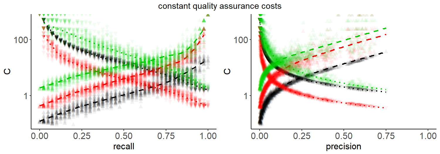
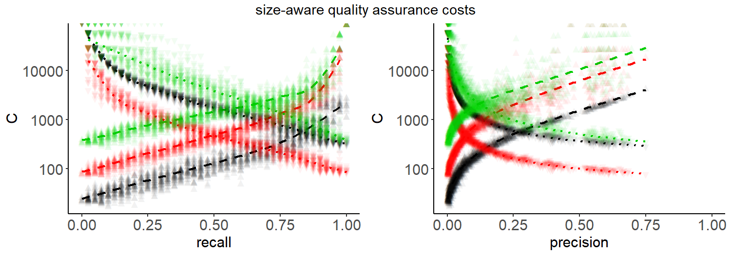
(b) zeppelin - medium difficulty defect prediction

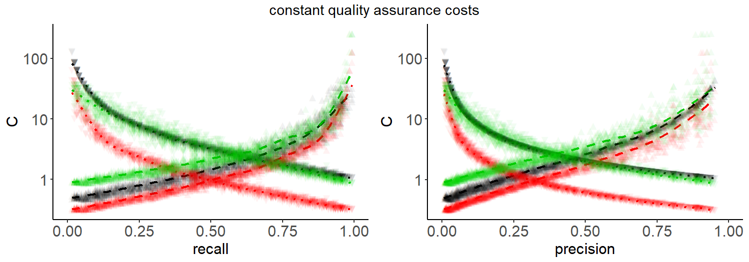
(c) falcon - imperfect quality assurance with $p_{qf}=0.5$

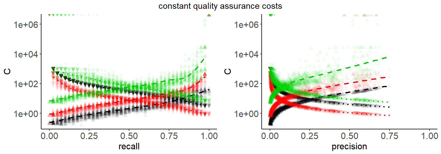
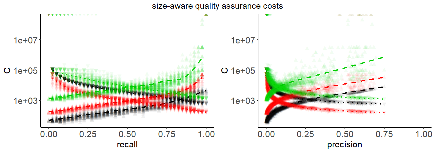
Figure 1: Trends of the upper and lower boundaries on the cost effectiveness. The lines show the regression of how the boundaries evolve in for changing values of recall and precision. The jitter shows the actual values of the experiments.

8 Discussion

While we evaluated our cost model only on simulated data and not on real defect prediction data sets, there are already several important insights that highlight the need for such a cost model for accurate evaluations of defect prediction models.

8.1 Impact of n-to-m relationships

There are large differences between the $n$-to-$m$, the $1$-to-$m$ and the 1-to-1 cost model. This is true both for the required performance of the models that allow for cost efficient predictions (i.e., lower boundary is less than upper boundary) as well as the range of values $C$ for which the prediction is cost saving. This effect is present for all projects we analyzed.

Thus, the results demonstrate that evaluations of defect prediction models may lead to wrong conclusions if the $n$-to-$m$ relationship between defects and artifacts is ignored. The estimated intervals for the cost ratio between defects and quality assurance for which defect prediction is cost efficient differs strongly from assuming 1-to-1 relationships. We expected this result due to multiple reasons:

• In the 1-to-1 relationship, the same defects may be counted as multiple distinct defects, i.e., once for each artifact that is affected.

• In the 1-to-1 relationship, defects may be ignored, i.e., if one artifact is affected by multiple defects.

To the best of our knowledge, there is no publication on defect prediction, that evaluates the results with respect to the $n$-to-$m$ relationship. This problem affects all current defect prediction research. To the best of our knowledge, there is only the work by Hemmati et al. [20], that exploits the $n$-to-$m$ relationship for the generation of a ranking of files. However, Hemmati et al. evaluate their study based on the density of remaining defects per file, i.e., they use an effort-aware 1-to-$m$ metric for the the evalution of their results. We note that all approaches from the state of the art can be evaluated with respect to the $n$-to-$m$ relationship, even if they completely ignore this property. This is possible, because our cost model only requires a binary function for labeling of single artifacts as defined in Equation (2). Regardless, algorithms that would already consider the $n$-to-$m$ relationship while fitting a prediction model, as is done by Hemmati et al. [20], are likely to perform better.

Moreover, the currently publicly available data sets do not contain the required information to evaluate $n$-to-$m$ relationships instead of 1-to-1 relationships. While some popular data sets (e.g., [23, 42]) contain defect counts and can be used for evaluations respecting the 1-to-$m$ relationship, others contain only binary labels and thus can only be used for 1-to-1 relationships (e.g., the NASA MDP data). The data published together with the RELINK approach is the only exception [43]. The prepared data for defect prediction only contains binary labels and, thus, only allows the evaluations with 1-to-1 relationships. However, the provided meta-data contains the links between all issues and commits, as well as the files that were touched in each commit. Thus, the generation of $n$-to-$m$ relationships would be possible with further processing of the meta data.

However, RELINK only contains data about four projects and only for three of them the complete data required for defect prediction are available. This is too few for realistic evaluations and, therefore, cannot be used to resolve this problem for our community. To resolve this problem, we require new public data sets for defect prediction research. With such new data, we can improve our evaluations to take the $n$-to-$m$ relationship into account and investigate the severity of ignoring this aspect in the last decades.

8.2 Relationship to confusion matrix based metrics

Our cost model is not unrelated to other performance measures. Our simulations already show that the boundaries are correlated with traditional measures like precision and recall. However, these correlations are not linear. For the constant cost model with 1-to-1 relationship between artifacts and defects and assuming perfect quality assurance, the lower boundary is actually the inverse of precision. The recall has no direct relationship with the cost boundaries. Due to the non-linearity of the relationship, an increase of, e.g., 10% recall does not mean that the costs are reduced by 10% or the boundaries change by 10%. For example, Figure 1(a) shows that if the recall for falcon is increased from 80% to 90%, there is a superlinear change of the upper boundary and a roughly linear change of the lower boundary. Thus, using such metrics for the comparison of models is - to some degree - a viable solution for the comparison of defect prediction models, even though the impact of the difference in performance metrics on costs may be misleading. However, our results also clearly show, that if only such metrics are considered, the crucial aspect of whether a prediction model can actually save costs is neglected.

8.3 Criteria for successful defect prediction

We consider defect prediction as successful if it can save costs. Our results show that there is no definitive value for metrics like precision and recall where defect prediction can be cost saving and that this is project dependent. For many projects we considered, a precision of less than 25% was sufficient for cost savings. Thus, criteria that define the success defect prediction using performance metrics like recall, precision, and accuracy are misleading (e.g., [44, 45, 4]). Using the boundary conditions of our cost model gives a hard criterion that is required for defect prediction to be successful, i.e., that the lower boundary must be less than the upper boundary.

8.4 The impact of the size

The trends for the size aware and constant cost model are almost the same, the difference is only the value for the cost ratio $C$, which is roughly shifted by multiplying the mean LOC of each project. This change is expected, as $C$ models the relation between quality assurance costs per complete artifacts and defects for the constant cost models, and the relation between the quality assurance costs per lines of code and defects for the size aware cost model. From the literature, we would have assumed that the differences between the size aware and the constant cost model are larger, e.g, because of the work by Rahman et al. [18]. However, our results indicate that while the size has an effect, the overall trend of how the boundaries behave is the same for the constant cost model and the size aware cost model. However, the reason for this lack of a stronger effect may be due to our randomized simulation of defect prediction models. Since size is often a strong predictor in defect prediction models, sometimes even outperforming machine learning [15], the results may change if prediction models that consider the size during predictions, are used.

8.5 Boundary conditions are required but not sufficient

While our boundary conditions are required for a positive profit they are not sufficient. Thus, even if the cost ratio of quality assurance efforts and defects of a project is within the interval of cost-saving cost ratios for a defect prediction model as defined by Corollary 3, it is possible that there is no positive profit. The reason for this is our assumption that the one-time and continuous costs are zero for our initializations. While we believe that these costs are relatively small (see Section 4.1), the interval between the upper and lower boundary decreases, as is shown by the corrolaries 1 and 2. Thus, if the actual cost ratio is very close to the boundaries, the actual profit could still be negative.

Additionally, our approach only considers success from the management perspective, i.e., related only to monetary issues. This does not cover whether software developers would actually use the defect prediction model as expected and what would be required to achieve this, as such considerations are out of scope of this article.

8.6 Using the cost model

Our work demonstrates the need for cost modeling of defect prediction models that goes beyond the standard measurements of prediction performance like precision and recall, because these measures are not directly related to the actual cost-saving potential of a defect prediction model. For the adoption of our cost model for future research, we propose the following.

1) Adopt the $n$-to-$m$ relationships. Our findings clearly show that the results of the realistic $n$-to-$m$ relationships between artifacts and defects deviate from the simple 1-to-1 and 1-to-n. Therefore either the size-aware or constant cost $n$-to-$m$ model should be used.

2) Evaluate if the prediction model is cost saving. All papers should evaluate if the lower bound is really less than the upper bound. If this is not the case, the defect prediction cannot save costs in comparison to one of the trivial baselines of either predicting nothing, or predicting everything.

3) Compare the upper and lower boundaries. In case different defect prediction models are compared to each other, the upper and lower boundaries are valuable metrics. We suggest that the boundaries are used instead of precision and recall for the comparison of models, as they give a more realistic picture on the actual performance of the prediction model in a realistic setting, because the relationship of the costs with precision and recall is not linear 8.2. Additionally, project managers can use the upper and lower boundaries to estimate if the defect prediction model can be cost saving in their project. Based on their intuition of what defects costs for the project, they can evaluate if the project/organization is within the cost saving area of the defect prediction model. The advantage of the boundaries is that project managers do not need to have exact estimates for the costs. If they can estimate a range in which the costs are, this is sufficient to evaluate if the defect prediction model can be cost saving.

4) Compare the range of cost saving ratios $C$. In addition to the comparison of the boundaries, the difference between the upper and the lower boundary should also be considered. We suggest that this comparison replaces performance measures like the $F-Measure$ as a large range of cost efficient values indicates that the model performs well under different circumstances. Moreover, the farther the actual cost ratio of a project is away from the boundaries, the higher the profit. Thus, defect prediction models with larger ranges between the boundaries are not only cost-savings for more projects, but can also save more costs.

5) Evaluate for perfect and imperfect quality assurance. Our results show that the cost efficiency of defect prediction models changes with the effectiveness of the applied quality assurance to reveal predicted defects. We suggest that both perfect (i.e., $p_{qf}=0$) as well as imperfect (e.g. $p_{qf}=0.5$) quality assurance is considered for evaluations.

8.7 Possible Improvements

While we believe that our general cost model covers the most important factors and the the initializions are based on reasonable assumptions, there may be opportunities to further improve the model.

On the one hand, the cost model could be initialized differently. In this case, Theorem 1 and corollaries 1 and 2 would not be affected. Then researchers could take pattern from Corrolory 3 and calculate the cost boundaries for the other initializations. For example, the costs for the quality assurance could be estimated in relation to the complexity of artifacts instead of the size, or even a combination of both. This way, the cost estimation could possibly better account for the impact of developer experience on the quality assurance costs.

On the other hand, there are several ways in which the general cost model may be extended. One possible extension would be to replace the constants $C_{EXEC}$ for continuous costs, $C_{QA}$ for the quality assurance costs per unit, and $C_{DEF}$ for the costs per defect with random variables. All three constants represent the mean costs that would occur. Consequently, these constants ignore the uncertainty in the probability distribution of these costs. A more realistic model would be to replace these constants with random variables that represent the probability distribution of these costs. This way, the cost model could account for randomly occurring continuous costs like the change of team members, respect that the quality assurance costs may vary per unit, and incorporate a more realistic model for the costs of defects. Mathematically, the current constants would be the expected value of the random variables, and, consequently, the cost boundaries we calculated would represent the expected cost boundaries. The random variables would enable a mathematical analysis of the uncertainty of these cost boundaries. However, a necessary precursor is that the probability distributions of these costs would be known, as the uncertainty of the costs could not be expressed otherwise.

Another possible extension is to incorporate additional cost factors into the cost model, e.g., drawbacks and benefits of the approach that are not directly associated to costs. For example, prediction models with a low precision may still be cost efficient, but they could potentially also be frustrating for developers due to the large amount of false positives. On the other hand, the developers would gain more experience with the artifacts that are false positives and they may also develop more (automated) tests for these artifacts. Thus, there would be an indirect gain in experience and possible future cost savings due to the larger test suite. Such cost terms could be added to the general model in Equation (5). As a consequence, Theorem 1 would have to account for these cost terms, which may modify the cost boundaries. A similar approach would be to subdivide the existing cost factors. E.g., the quality assurance costs could be divided into the costs due a potentially delayed release and the costs for additional man power required for the quality assurance. Alternatively, the cost model could be used as is, but instantiated twice: once with only man power considerations, once with only time considerations. This would allow managers to evaluate if the prediction model may be more expensive in terms of man power, but effective in terms of loss due to a delayed release.

A further possible extension of the cost model is to subdivide the cost factors, e.g., to subdivide the costs of defects into costs for security issues, costs for defects that crash the application, and costs for other defects. However, this extension is incompatible with the mathematical analysis we conducted in this article. We were only able to proof the boundary conductions because we could reduce the number of unknown variables to one by considering the costs for quality assurance and the costs for defects as a ratio. If we would, e.g., subdivide the costs of defects into three subcategories, we would have three such ratios as unknown variables and would need to establish boundary conditions for these variables that would not be independent of each other. Thus, we do not believe that such an extension of this cost model is feasible. Regardless, if random variables are used as we described at the beginning of this section, the distribution of the random variable could account for the different types of defects, e.g., by modelling the distribution of the cost of defects as a mixture of the distributions of the costs of security issues, costs of crashes, and costs of other defects.

8.8 Threats to Validity

There are several threats to the validity of our work, which we report following the classification by Wohlin et al. [46].

8.8.1 Construct Validity

The evaluation of the boundary conditions through simulation of defect predictions may be unsuited for the evaluation of trends. We mitigated this by simulating the prediction an real-world data and sampling accross a large range of prediction performances. There may be a defect in the code for the simulations of defect prediction and the evaluation of them using our cost model for the experiments performed in Section 7. However, the source code is relatively short and not very complex. Moreover, we reviewed the source code to minimize this possibility.

8.8.2 Internal Validity

There may be important factors influencing the costs of defect predictions, which we did not include in the general model. We scanned the literature regarding related work to costs of defect predictions to mitigate this threat. Moreover, we initialized the cost model using different assumptions. These assumptions may be unrealistic or wrong, leading to wrong conclusions. We explained the rationale behind each design decision and, if possible, grounded them in prior work from the literature to mitigate this threat.

We have only presented the results of the trends of the cost model with respect to precision and recall, because these are the most common metrics used for defect prediction research. These trends may look different using other metrics. However, other common metrics are either directly or indirectly related to precision and recall, e.g., the F-Measure, G-Measure, or AUC. This mitigates the threat that our conclusions, especially regarding the impact of the $n$-to-$m$ relationship may be wrong.

The collected data may also contain problems we have not addressed causing noise in the data. Commits may reference multiple issues, which could lead to double counting of files for defects. However, only 46 of the 1493 commits that address defects reference multiple issues, i.e., the effect of this would be very small.

Moreover, we have not manually validated that all changes within a commit that fixes a defect are really part of the correction of the defect. This means that our data may have an inflated number of files per defect, which could bias the results towards showing differences between the $n$-to-$m$ cost model and the 1-to-1 and the 1-to-$m$ cost model. To mitigate this threat, we cross-checked our ratio of files per defect $mean(|d|)$ with the results by Mills et al. [47], who manually validated the file actions. Based on the results by Mills et al., $mean(|d|)$ falls into the interval $[1.11,2.13]$ with 99.5% confidence. Our data has a mean value of 1.56. Thus, even if there are false positive file actions in our data, the results from the experiment should still be representative.

Additionally, we took a closer look at the projects tika and zookeeper, as Mills et al. [47] manually validated data from these projects, although from a different time period than our data. We evaluated how many changes to files Mills et al. manually determined as part of the correction of a defect and compared this to the number of of changes to files that we identify with our heuristic for the removal of false positive file changes based on changes to whitespaces, comments, and tests. For tika, Mills et al. identified 22 changes to files for the correction of defects and 27 changes to files that were unrelated to defects. We correctly filtered 22 of the 27 unrelated changes. For zookeeper, Mills et al. identified 114 changes to files for the correction of defects and 126 unrelated changes. We correctly filtered 98 of the 126 unrelated changes. Overall, we filtered 78% of the unrelated changes. Thus, we removed most of the noise from our data. Consequently, it is highly unlikely that the remaining noise is strong enough to alter our results to such a degree that no differences due to the $n$-to-$m$ relationship would be visible anymore.

8.8.3 External Validity

While we evaluated our cost model on fifteen real-world projects, we only used simulation and did not use actual defect prediction models. From our results, we extrapolate that our cost model is required and can affect the results of evaluations for all real-world project where a subset of the defects affect multiple files, due to the $n$-to-$m$ relationship. However, we cannot definitively conclude this.

8.8.4 Reliability

The filtering of issues whether they are really defects or not may affect the results of this article and depends on the author. To mitigate this threat to the reliability, we followed the same rules for defects as Herzig et al. [41] and documented all decisions in the replication kit. Due to the results of Herzig et al. [41], we expected to discard between 27.4% and 42.9% of the issues with 99.5% confidence. Thus, the $\frac{175}{413}=42.4\%$ discarded issues are within the bounds established by the state of the art, indicating that this study is reliable.

9 Conclusion

In this article, we specified a cost model for software defect prediction, showed how the cost model can be used to calculate the profit of defect prediction, and defined mathematically provable boundaries that defect prediction must fulfill in order to allow for a positive profit under any circumstances. We have shown how our cost model can be initialized using different assumptions. Using simulated defect prediction data, we have analyzed the impact of the assumptions on the costs. Using these insights, we provide guidelines for using our cost model in future research. Moreover, we discovered a flaw in all current defect prediction data sets and consequently also all evaluations of defect prediction approaches due to an oversimplification of the relationship between software artifacts and defects.

In future work, we will apply our cost model to the state of the art of defect prediction and assess under which conditions the predictions are successful and compare defect prediction models with respect to their cost-saving potential. However, before such an analysis is possible, we will work on creating a new defect prediction data set that allows for evaluations that respect the $n$-to-$m$ relationship between software artifacts and defects as our simulations show that cost estimation are very different if this aspect is not considered. Another important aspect of future work are measures for the acceptance of defect prediction models by develepors. While the profit is an imporant indicator for success of a technique from the management perspective, tools that apply defect prediction must be used by developers. For example, our results show that a positive profit can sometimes be achieved even with a low precision, i.e., many false positives. However, whether developers would accept this and under which circumstances they may accept a high number of false positives has not yet been sufficiently addressed in the literature.

Steffen Herbold PD Dr. Steffen Herbold currently manages a Machine Learning professorship at the Institute of Computer Science of the Georg-August-Universität Göttingen. His research is focused on the application of data science methods and their applications in software engineering as well as software engineering to data science methods.

References

- [1] C. Catal and B. Diri, “A systematic review of software fault prediction studies,” Expert Systems with Applications, vol. 36, no. 4, pp. 7346 – 7354, 2009.
- [2] T. Hall, S. Beecham, D. Bowes, D. Gray, and S. Counsell, “A systematic literature review on fault prediction performance in software engineering,” IEEE Trans. Softw. Eng., vol. 38, no. 6, pp. 1276–1304, Nov. 2012.
- [3] S. Hosseini, B. Turhan, and D. Gunarathna, “A systematic literature review and meta-analysis on cross project defect prediction,” IEEE Trans. Softw. Eng., p. 1, 2017.
- [4] S. Herbold, A. Trautsch, and J. Grabowski, “A comparative study to benchmark cross-project defect prediction approaches,” IEEE Trans. Softw. Eng., vol. PP, no. 99, pp. 1–1, 2017.
- [5] J. Nam, W. Fu, S. Kim, T. Menzies, and L. Tan, “Heterogeneous defect prediction,” IEEE Trans. Softw. Eng., vol. PP, no. 99, pp. 1–1, 2017.
- [6] X. Jing, F. Wu, X. Dong, F. Qi, and B. Xu, “Heterogeneous cross-company defect prediction by unified metric representation and cca-based transfer learning,” in Proc. of the 2015 10th Joint Meeting on Foundations of Software Engineering, ser. ESEC/FSE 2015. New York, NY, USA: ACM, 2015, pp. 496–507.
- [7] J. Nam and S. Kim, “Clami: Defect prediction on unlabeled datasets,” in Automated Software Engineering (ASE), 2015 30th IEEE/ACM Int. Conf. on, Nov 2015, pp. 452–463.
- [8] F. Zhang, Q. Zheng, Y. Zou, and A. E. Hassan, “Cross-project defect prediction using a connectivity-based unsupervised classifier,” in Proc. of the 38th Int. Conf. on Software Engineering. ACM, 2016.
- [9] Q. Huang, X. Xia, and D. Lo, “Supervised vs unsupervised models: A holistic look at effort-aware just-in-time defect prediction,” in 2017 IEEE Int. Conf. on Software Maintenance and Evolution (ICSME), Sept 2017, pp. 159–170.
- [10] C. Tantithamthavorn, S. McIntosh, A. E. Hassan, and K. a. Matsumoto, “An empirical comparison of model validation techniques for defect prediction models,” IEEE Trans. Softw. Eng., vol. 43, no. 1, pp. 1–18, 2017.
- [11] C. Tantithamthavorn, S. McIntosh, A. E. Hassan, and K. Matsumoto, “Automated parameter optimization of classification techniques for defect prediction models,” in Proc. of the 38th Int. Conf. on Software Engineering. ACM, 2016.
- [12] R. Krishna and T. Menzies, “Bellwethers: A baseline method for transfer learning,” IEEE Trans. Softw. Eng., pp. 1–1, 2018.
- [13] C. Tantithamthavorn and A. E. Hassan, “An experience report on defect modelling in practice: Pitfalls and challenges,” The Int. Conf. on Software Engineering: Software Engineering in Practice Track (ICSE-SEIP), vol. 15, no. 17, pp. 71–73, 2018.
- [14] Y. Yang, Y. Zhou, J. Liu, Y. Zhao, H. Lu, L. Xu, B. Xu, and H. Leung, “Effort-aware just-in-time defect prediction: Simple unsupervised models could be better than supervised models,” in Proc. of the 2016 24th ACM SIGSOFT Int. Symp. on Foundations of Software Engineering. ACM, 2016.
- [15] Y. Zhou, Y. Yang, H. Lu, L. Chen, Y. Li, Y. Zhao, J. Qian, and B. Xu, “How far we have progressed in the journey? an examination of cross-project defect prediction,” ACM Trans. Softw. Eng. Methodol., vol. 27, no. 1, pp. 1:1–1:51, Apr. 2018.
- [16] S. Herbold, “A systematic mapping study on cross-project defect prediction,” CoRR, vol. abs/1705.06429, 2017. [Online]. Available: https://arxiv.org/abs/1705.06429
- [17] N. Ohlsson and H. Alberg, “Predicting fault-prone software modules in telephone switches,” IEEE Trans. Softw. Eng., vol. 22, no. 12, pp. 886–894, Dec. 1996.
- [18] F. Rahman, D. Posnett, and P. Devanbu, “Recalling the “imprecision” of cross-project defect prediction,” in Proc. ACM SIGSOFT 20th Int. Symp. Found. Softw. Eng. (FSE). ACM, 2012.
- [19] Y. Jiang, B. Cukic, and Y. Ma, “Techniques for evaluating fault prediction models,” Empirical Softw. Eng., vol. 13, no. 5, pp. 561–595, 2008.
- [20] H. Hemmati, M. Nagappan, and A. E. Hassan, “Investigating the effect of ”defect co-fix” on quality assurance resource allocation: A search-based approach,” Journal of Systems and Software, vol. 103, pp. 412 – 422, 2015.
- [21] E. Arisholm and L. C. Briand, “Predicting fault-prone components in a Java legacy system,” in Proc. 5th ACM/IEEE Int. Symp. Emp. Softw. Eng. (ISESE). ACM, 2006.
- [22] G. Canfora, A. D. Lucia, M. D. Penta, R. Oliveto, A. Panichella, and S. Panichella, “Multi-objective cross-project defect prediction,” in Proc. 6th IEEE Int. Conf. Softw. Testing, Verification and Validation (ICST), 2013.
- [23] M. Jureczko and L. Madeyski, “Towards identifying software project clusters with regard to defect prediction,” in Proc. 6th Int. Conf. on Predictive Models in Softw. Eng. (PROMISE). ACM, 2010.
- [24] Y. Zhang, D. Lo, X. Xia, and J. Sun, “An empirical study of classifier combination for cross-project defect prediction,” in Computer Software and Applications Conf. (COMPSAC), 2015 IEEE 39th Annual, vol. 2, July 2015, pp. 264–269.
- [25] T. M. Khoshgoftaar and E. B. Allen, “Classification of fault-prone software modules: Prior probabilities, costs, and model evaluation,” Emp. Softw. Eng., vol. 3, no. 3, pp. 275–298, Sep 1998.
- [26] T. M. Khoshgoftaar and N. Seliya, “Comparative assessment of software quality classification techniques: An empirical case study,” Emp. Softw. Eng., vol. 9, no. 3, pp. 229–257, Sep 2004.
- [27] C. Drummond and R. Holte, “Cost curves: An improved method for visualizing classifier performance,” Machine Learning, vol. 65, no. 1, pp. 95–130, 2006.
- [28] H. Zhang and S. C. Cheung, “A cost-effectiveness criterion for applying software defect prediction models,” in Proc. of the 2013 9th Joint Meeting on Foundations of Software Engineering, ser. ESEC/FSE 2013. New York, NY, USA: ACM, 2013, pp. 643–646.
- [29] H. Pham, “Software reliability and cost models: Perspectives, comparison, and practice,” European Journal of Operational Research, vol. 149, no. 3, pp. 475 – 489, 2003.
- [30] J. Kingman, Poisson Processes. Clarendon Press, 1992, vol. 3.
- [31] S. J. Stolfo, Wei Fan, Wenke Lee, A. Prodromidis, and P. K. Chan, “Cost-based modeling for fraud and intrusion detection: results from the jam project,” in Proc. DARPA Information Survivability Conf. and Exposition. DISCEX’00, vol. 2, Jan 2000, pp. 130–144 vol.2.
- [32] G. Patry, A. Romagny, S. Martinet, and D. Froelich, “Cost modeling of lithium-ion battery cells for automotive applications,” Energy Science & Engineering, vol. 3, no. 1, pp. 71–82, 2015.
- [33] D. S. Etkin, “Modeling oil spill response and damage costs,” in Proc. of the Fifth Biennial Freshwater Spills Symp., 2004.
- [34] M. Pugliatti, E. Beghi, L. Forsgren, M. Ekman, and P. Sobocki, “Estimating the cost of epilepsy in europe: A review with economic modeling,” Epilepsia, vol. 48, no. 12, pp. 2224–2233, 2007.
- [35] E. Nakamura and J. Steinsson, “Monetary Non-neutrality in a Multisector Menu Cost Model*,” The Quarterly Journal of Economics, vol. 125, no. 3, pp. 961–1013, 08 2010.
- [36] G. Canfora, A. D. Lucia, M. D. Penta, R. Oliveto, A. Panichella, and S. Panichella, “Defect prediction as a multiobjective optimization problem,” Software Testing, Verification and Reliability, vol. 25, no. 4, pp. 426–459, 2015.
- [37] M. D’Ambros, M. Lanza, and R. Robbes, “Evaluating defect prediction approaches: A benchmark and an extensive comparison,” Empirical Softw. Engg., vol. 17, no. 4-5, pp. 531–577, Aug. 2012.
- [38] S. Hosseini, B. Turhan, and M. Mäntylä, “A benchmark study on the effectiveness of search-based data selection and feature selection for cross project defect prediction,” Information and Software Technology, 2017.
- [39] F. Trautsch, S. Herbold, P. Makedonski, and J. Grabowski, “Addressing problems with replicability and validity of repository mining studies through a smart data platform,” Emp. Softw. Eng., Aug 2017.
- [40] S. Herbold, “sherbold/replication-kit-tse-2018-costmodel: Release of the replication kit,” Nov 2019. [Online]. Available: https://doi.org/10.5281/zenodo.3537703
- [41] K. Herzig, S. Just, A. Rau, and A. Zeller, “Predicting defects using change genealogies,” in Software Reliability Engineering (ISSRE), 2013 IEEE 24th Int. Symp. on, Nov 2013, pp. 118–127.
- [42] M. D’Ambros, M. Lanza, and R. Robbes, “An Extensive Comparison of Bug Prediction Approaches,” in Proc. of the 7th IEEE Working Conf. on Mining Software Repositories (MSR). IEEE Computer Society, 2010.
- [43] R. Wu, H. Zhang, S. Kim, and S.-C. Cheung, “Relink: Recovering links between bugs and changes,” in Proc. of the 19th ACM SIGSOFT Symp. and the 13th European Conf. on Foundations of Software Engineering, ser. ESEC/FSE ’11. New York, NY, USA: ACM, 2011, pp. 15–25.
- [44] T. Zimmermann, N. Nagappan, H. Gall, E. Giger, and B. Murphy, “Cross-project defect prediction: a large scale experiment on data vs. domain vs. process,” in Proc. the 7th Joint Meet. Eur. Softw. Eng. Conf. (ESEC) and the ACM SIGSOFT Symp. Found. Softw. Eng. (FSE). ACM, 2009, pp. 91–100.
- [45] Z. He, F. Shu, Y. Yang, M. Li, and Q. Wang, “An investigation on the feasibility of cross-project defect prediction,” Automated Softw. Eng., vol. 19, pp. 167–199, 2012.
- [46] C. Wohlin, P. Runeson, M. Höst, M. C. Ohlsson, B. Regnell, and A. Wesslen, Experimentation in Software Engineering. Springer Publishing Company, Incorporated, 2012.
- [47] C. Mills, J. Pantiuchina, E. Parra, G. Bavota, and S. Haiduc, “Are bug reports enough for text retrieval-based bug localization?” in 2018 IEEE Int. Conf. on Software Maintenance and Evolution (ICSME), Sep. 2018, pp. 381–392.